Learning Combinations of Sigmoids
Through Gradient Estimation

Abstract

We develop a new approach to learn the parameters of regression models with hidden variables. In a nutshell, we estimate the gradient of the regression function at a set of random points, and cluster the estimated gradients. The centers of the clusters are used as estimates for the parameters of hidden units. We justify this approach by studying a toy model, whereby the regression function is a linear combination of sigmoids. We prove that indeed the estimated gradients concentrate around the parameter vectors of the hidden units, and provide non-asymptotic bounds on the number of required samples. To the best of our knowledge, no comparable guarantees have been proven for linear combinations of sigmoids.

1 Introduction

Classification and regression models with hidden variables have a long history in statistical learning. They naturally arise when learning mixtures, a topic recently receiving considerable attention (Chaganty and Liang, 2013; Sun et al., 2014; Anandkumar et al., 2012, 2014; Hsu and Kakade, 2013). Interest on such models has also increased because of the empirical success of deep neural networks in image and speech processing tasks (Bengio, 2009; Krizhevsky et al., 2012; Hinton et al., 2012). One of the most striking properties of these models is the ability to learn high-level representations that are particularly useful for discriminative purposes (Boureau et al., 2008; Mairal et al., 2009; Boureau et al., 2010; Yu et al., 2013; Humphrey et al., 2013). This ability–often referred to as ‘feature learning’–is yet poorly understood. From a modeling point of view, it is unclear what are the key elements of such high-level representations, and how are they captured (for instance) by deep neural networks. From a computational point of view, the corresponding empirical risk minimization problem is highly non-convex, and it is unclear why existing algorithms are empirically successful at learning these representations.

In this work, we consider a regression model with response variable $y\in{\mathbb{R}}$ and covariates ${\boldsymbol{x}}\in{\mathbb{R}}^{d}$, linked through the regression function:

$${\mathbb{E}}\big{\{}y|{\boldsymbol{x}}\big{\}}\equiv r({\boldsymbol{x}})=\textstyle\sum_{\ell=1}^{k}u_{\ell}\,f(\langle{\boldsymbol{w}}^{\ell},{\boldsymbol{x}}\rangle)\,,$$ (1)

where, ${\boldsymbol{w}}^{1},\dots,{\boldsymbol{w}}^{k}\in{\mathbb{R}}^{d}$, $u_{1},\dots,u_{k}\in{\mathbb{R}}$, $f:{\mathbb{R}}\to{\mathbb{R}}$ is the sigmoid $f(x)=\tanh(\beta x)=\frac{e^{\beta x}-e^{-\beta x}}{e^{\beta x}+e^{-\beta x}},$ for some $\beta>0$, and $\langle{\boldsymbol{a}},{\boldsymbol{b}}\rangle=\sum_{i=1}^{d}a_{i}b_{i}$ is the usual scalar product in ${\mathbb{R}}^{d}$. In the general case, the weights $u_{\ell}$, $\ell\in[k]\equiv\{1,\ldots,k\}$ have arbitrary signs, while in the mixture case, they are positive and sum to one. Our objective is to learn the parameter vectors $\{{\boldsymbol{w}}^{\ell}\}_{\ell=1}^{k}$, particularly when $k\ll d$; it is useful to pause for a few remarks on this model:

• In the general case, learning the parameter vectors $\{{\boldsymbol{w}}^{\ell}\}_{\ell=1}^{k}$ can be viewed as a simple model for feature learning. In particular, (1) corresponds to a two-layer neural network with $k$ hidden units. The non-linear functions $f(\langle{\boldsymbol{w}}^{1},\cdot\rangle)$, $f(\langle{\boldsymbol{w}}^{2},\cdot\rangle)$, …, $f(\langle{\boldsymbol{w}}^{k},\cdot\rangle)$, provide a high-level, lower-dimensional representation of the data.

• In the mixture case, (1) is the expected label generated by a mixture of $k$ logistic classifiers, each selected with probability $u_{\ell}$. Each vector ${\boldsymbol{w}}^{\ell}$ is the normal to the separating hyperplane defining each classifier; learning $\{{\boldsymbol{w}}^{\ell}\}_{\ell=1}^{k}$ thus corresponds to learning the mixture’s constituent distributions. When $k\ll d$, the number of classifiers (or ‘modes’) is smaller than the ambient dimension, as is the case in many applications (Sun et al., 2014; Yi et al., 2014; Chen et al., 2014).

• In both cases, once $\{{\boldsymbol{w}}^{\ell}\}_{\ell=1}^{k}$ are known, learning the full regression function is straightforward: fitting $\{u_{\ell}\}_{\ell=1}^{k}$ is a standard linear regression problem.

Our approach is based on a simple remark. The gradient of the regression function $r$ at any ${\boldsymbol{\xi}}\in{\mathbb{R}}^{d}$ is a linear combination of $\{{\boldsymbol{w}}^{\ell}\}_{\ell=1}^{k}$, with coefficients depending on ${\boldsymbol{\xi}}$, i.e., $\nabla r({\boldsymbol{x}})=\sum_{\ell=1}^{k}c_{\ell}({\boldsymbol{\xi}})\,{\boldsymbol{w}}^{\ell}\,$ (see Section 3.2). Further, if ${\boldsymbol{\xi}}$ is sufficiently far from the origin, this linear combination is typically sparse: it contains at most one non-vanishing coefficient. Our algorithm thus proceeds in two steps: $(1)$ estimate the gradient $\nabla r(\,\cdot\,)$ at $m_{0}$ random positions ${\boldsymbol{\xi}}^{1}$, …, ${\boldsymbol{\xi}}^{m_{0}}$; $(2)$ cluster these estimates and use cluster centers as estimates of $\{{\boldsymbol{w}}^{\ell}\}_{\ell=1}^{k}$.

Our main technical contribution is to prove that this approach is consistent: for large $m_{0}$, the algorithm generates gradient estimates that concentrate around ${\boldsymbol{w}}^{1}$, …, ${\boldsymbol{w}}^{k}$. We establish non-asymptotic bounds on the minimum sample size that guarantees this clustering to take place. We do so under three different methods for estimating $\nabla r(\cdot)$. Assuming access to a value oracle for $r$, we construct a gradient estimator under which clustering succeeds with only $\Theta(d)$ oracle calls. Assuming access to covariates ${\boldsymbol{x}}$ sampled from a standard Gaussian distribution, we show that clustering succeeds with access to $e^{\Theta(d)}$ samples in the general case. A dimensionality reduction method by Sun et al. (2014) allows us to reduce the complexity to $\Theta(d)+e^{\Theta(\mathtt{poly}(k))}$ samples, in the mixture case (i.e., $\{u_{\ell}\}_{\ell=1}^{k}$ positive and summing to one).

The rest of the paper is organized as follows. In Section 2, we review related work in the area. Section 3 describes in detail the new algorithm. In Section 4 we state our main results. Finally, we outline our proof in Section 5, with many technical details deferred to the appendix.

2 Related Work

Typical approaches to learning mixtures, like EM (Dempster et al., 1977) come with no guarantees, and suffer from convergence to local minima. Providing guarantees for even the idealized case of learning mixtures of Gaussians is non-trivial, and has been the subject of several recent studies (Moitra and Valiant, 2010; Hsu and Kakade, 2013). There are relatively few rigorous results that guarantee learning for regression models with latent variables. Chaganty and Liang (2013) consider mixtures of linear regressions. In this setting, they show that regressing the response from second and third order tensors of the covariates yields coefficients, also higher order tensors, whose decomposition reveals the model parameters. A different approach, relying only on the second-order tensor (i.e., the covariance) and alternating minimization is followed by Yi et al. (2014) , for a mixture composed of two linear models in the absence of noise; the same setting, in the presence of noise, is studied by Chen et al. (2014). None of these approaches can be applied to our model: our components are non-linear (sigmoids), while the above works focus on linear components; moreover, both Yi et al. (2014) and Chen et al. (2014) limit their analysis to $k=2$ hidden units.

Sedghi and Anandkumar (2016) apply the moment method, as well as tensor factorization techniques, to learn mixtures of sigmoids. Their contribution is not directly comparable to ours: they assume the vectors ${\boldsymbol{w}}^{\ell}$ are random, and require a special non-degeneracy condition on the expectations of third derivatives of the hidden units. For instance, this condition is not satisfied by $f(x)=\tanh(\beta x)$ if ${\boldsymbol{x}}$ has a symmetric distribution. Sun et al. (2014) consider the problem of learning a mixture of linear classifiers, and provide guarantees for learning the subspace spanned by $\{{\boldsymbol{w}}^{\ell}\}_{\ell=1}^{k}$. This, in turn, can be used for dimensionality reduction: projecting the covariates to this space reduces the problem dimension from $d$ to $k$. We focus on learning the parameter vectors, rather than their span; our contribution is thus complementary to Sun et al. (2014). In fact, we exploit their result to reduce our algorithm’s complexity under Gaussian covariates.

Our approach can be cast as a means to learn the parameters of a two-stage neural network. Such networks are known to be quite expressive (Barron, 1993), in that they can approximate arbitrary polynomials. A recent result by Andoni et al. (2014) shows that, in the presence of a large number of neurons with random parameter vectors, a polynomial can be learned through gradient descent. Our contribution differs in two important directions: $(i)$ we want to learn the hidden-unit parameter vectors, rather than approximate a given regression function, and $(ii)$ we develop explicit bounds on the sample size, while Andoni et al. (2014) assume infinite sample size $n=\infty$. Namely, they assume access to the gradient of the regression function: a substantial part of our technical work is devoted to proving this can be sufficiently estimated. Arora et al. (2014) prove that certain very sparse deep neural networks with random connection patterns can be learned in polynomial time and sample complexity. In model (1), this would correspond to random, sparse vectors ${\boldsymbol{w}}^{\ell}$, $\{u_{\ell}\}_{\ell=1}^{k}$. Their techniques do not seem applicable to non-random connections or to non-sparse graphs. Finally, there are several celebrated results on the sample complexity of approximating a function through a neural network (see, e.g., Anthony and Bartlett (2009)). This is a different problem than the parameter estimation problem we solve here. A formal understanding of parameter estimation is crucial in understanding why neural nets learn low-dimensional representations well. Parameter estimation also naturally arises in learning mixtures, where correctly identifying the constituent components (or, modes) is of equal or greater importance than regressing the mixture function.

3 Modelling Assumptions and Learning Algorithm

3.1 Modeling Assumptions

Recall that we consider a regression model with response variable $y\in{\mathbb{R}}$, generated through (1) from covariates ${\boldsymbol{x}}\in{\mathbb{R}}^{d}$. Note that (1) is equivalent to $y=\sum_{\ell=1}^{k}u_{\ell}\,f(\langle{\boldsymbol{w}}^{\ell},{\boldsymbol{x}}\rangle)+{\varepsilon}\,,$ with ${\varepsilon}$ a noise term such that ${\mathbb{E}}\{{\varepsilon}|{\boldsymbol{x}}\}=0$. In the general case, we assume that for any $\ell\in[k]\equiv\{1,\ldots,k\}$, the vectors ${\boldsymbol{w}}^{\ell}$ have unit norm, i.e., $\|{\boldsymbol{w}}^{\ell}\|_{2}=1$, the absolute value of each weight is at most one, i.e., $u_{\ell}\in[-1,1]$, and the response is bounded, i.e., $y\in[-M,M]$ for some $M>0$. In the mixture case, we assume in addition that $u_{\ell}\geq 0$, $l\in[k]$, and $\sum_{\ell=1}^{k}u_{\ell}=1.$

Clearly, we cannot learn a vector ${\boldsymbol{w}}^{\ell}$ if $u_{\ell}=0$, nor distinguish two vectors ${\boldsymbol{w}}^{\ell},{\boldsymbol{w}}^{\ell^{\prime}}$, where $\ell\neq\ell^{\prime}$, if they are identical. For this reason, we make the following two additional assumptions. First, coefficients $u_{\ell}$ are bounded away from zero, i.e., there exists a $u_{0}$ s.t. $0<u_{0}\leq|u_{\ell}|<1$, for all $\ell\in[k]$. Second, the collinearity between any subset of vectors ${\boldsymbol{w}}^{\ell}$ is also bounded. Formally, let ${\boldsymbol{M}}=[{\boldsymbol{w}}^{1}|{\boldsymbol{w}}^{2}|\cdots|{\boldsymbol{w}}^{k}]\in{\mathbb{R}}^{d\times k}$ be the matrix comprising the vectors ${\boldsymbol{w}}^{\ell}$ column-wise. We assume that there exists a $\kappa>0$ such that $\kappa\leq\sigma_{\rm min}({\boldsymbol{M}})$, where $\sigma_{\rm min}$ the smallest singular value of ${\boldsymbol{M}}$. Intuitively, the existence of $\kappa$ implies a lower bound on the angle between any two vectors ${\boldsymbol{w}}^{\ell},{\boldsymbol{w}}^{\ell^{\prime}}$.

Our learning method relies on producing estimates of the gradient $\nabla r(\cdot)$ at arbitrary points in ${\mathbb{R}}^{d}$. We produce estimators of the gradient under two different models on our ability to sample function $r$:

• Value Oracle Model. Under our first model, we assume access to a value oracle: given a ${\boldsymbol{x}}\in{\mathbb{R}}^{d}$, the oracle produces a $y\in{\mathbb{R}}$ governed by (1), while successive calls to the oracle are independent. Put differently, we treat (1) as a ‘black box’, whose inputs are under our algorithm’s control.

• Gaussian Covariates Model. Under our second model, we assume that the covariates ${\boldsymbol{x}}$ follow a standard Gaussian ${\sf N}(0,{\rm I}_{d\times d})$, while $y$ is given by (1). Our learning algorithm has access to $n$ independent pairs $({\boldsymbol{x}}^{(1)},y^{(1)})$, …, $({\boldsymbol{x}}^{(n)},y^{(n)})$ generated from the above joint distribution, and must construct gradient estimates $\nabla r({\boldsymbol{\xi}})$ at different ${\boldsymbol{\xi}}\in{\mathbb{R}}^{d}$ from this dataset alone.

3.2 Intuition Behind our Approach

Consider the gradient of the expected response function $r:{\mathbb{R}}^{d}\to{\mathbb{R}}$, evaluated at a ${\boldsymbol{\xi}}\in{\mathbb{R}}^{d}$:

$$\nabla r({\boldsymbol{\xi}})=\textstyle\sum_{\ell=1}^{k}u_{\ell}f^{\prime}(\langle{\boldsymbol{w}}^{\ell},{\boldsymbol{\xi}}\rangle)\cdot{\boldsymbol{w}}^{\ell}\,$$ (2)

Observe that $\nabla r({\boldsymbol{\xi}})$ is a linear combination of the parameter vectors ${\boldsymbol{w}}^{\ell}$. Moreover, since $f$ is a sigmoid, $\lim_{|t|\to\infty}f^{\prime}(t)=0$. Thus, for any ${\boldsymbol{\xi}}$ such that $|\langle{\boldsymbol{w}}^{\ell},{\boldsymbol{\xi}}\rangle|\gg 1$, the coefficient $u_{\ell}f^{\prime}(\langle{\boldsymbol{w}}^{\ell},{\boldsymbol{\xi}}\rangle)$ weighing the contribution of ${\boldsymbol{w}}^{\ell}$ to the gradient $\nabla r({\boldsymbol{\xi}})$ is small. As a result, ${\boldsymbol{w}}^{\ell}$ contributes significantly to the gradient $\nabla r({\boldsymbol{\xi}})$ when it is approximately normal to ${\boldsymbol{\xi}}$, i.e., $|\langle{\boldsymbol{w}}^{\ell},{\boldsymbol{\xi}}\rangle|\approx 0$.

These observations motivate our approach. Presuming the existence of an estimator of the gradient, our algorithm amounts to the following three steps:

• Pick several ${\boldsymbol{\xi}}\in{\mathbb{R}}^{d}$, and produce estimates of the gradient ${\boldsymbol{w}}({\boldsymbol{\xi}})\approx\nabla r({\boldsymbol{\xi}})$.

• If $\|{\boldsymbol{w}}({\boldsymbol{\xi}})\|_{2}$ is below a threshold $w_{0}$, ignore this estimate. Otherwise, normalize it, producing ${\boldsymbol{\tilde{w}}}({\boldsymbol{\xi}})={\boldsymbol{w}}({\boldsymbol{\xi}})/\|{\boldsymbol{w}}({\boldsymbol{\xi}})\|_{2}$.

• Identify $k$ clusters among the resulting ‘candidate’ vectors ${\boldsymbol{\tilde{w}}}({\boldsymbol{\xi}})$, and report the centers of these $k$ clusters as the parameter vector estimates for $\{{\boldsymbol{w}}^{\ell}\}_{\ell=1}^{k}$.

If a ${\boldsymbol{w}}({\boldsymbol{\xi}})$ has a high norm, then ${\boldsymbol{\xi}}$ must be approximately normal to at least one vector in $\{{\boldsymbol{w}}^{\ell}\}_{\ell=1}^{k}$. Moreover, if it is approximately normal to only one such vector, say ${\boldsymbol{w}}^{1}$, by (2) the estimated gradient ${\boldsymbol{w}}({\boldsymbol{\xi}})$ will have a significant component in the direction of ${\boldsymbol{w}}^{1}$. As such, after renormalization, all such vectors are indeed clustered around ${\boldsymbol{w}}^{1}$. Our formal guarantees, as stated by Theorem 1, establish that most candidates indeed satisfy this property, with the exception of a small spurious set.

3.3 Gradient Estimation

The above approach crucially relies on estimating the response gradient $\nabla r(\cdot)$ at an arbitrary ${\boldsymbol{\xi}}\in{\mathbb{R}}^{d}$. We discuss our estimation process for each of the two models below.

• Gradient Estimation in the Value Oracle Model. Under the Value Oracle model, given a ${\boldsymbol{\xi}}\in{\mathbb{R}}^{d}$, we generate $n_{0}$ i.i.d. pairs $({\boldsymbol{x}}^{(i)},y^{(i)})$ where each ${\boldsymbol{x}}^{(i)}$ is sampled from ${\sf N}({\boldsymbol{\xi}},{\rm I}_{d\times d})$, and $y^{(i)}$ is the corresponding value returned by the oracle. The estimate ${\boldsymbol{w}}({\boldsymbol{\xi}})$ of $\nabla r({\boldsymbol{\xi}})$ is then:

  $${\boldsymbol{w}}({\boldsymbol{\xi}})=\textstyle\frac{1}{n_{0}}\sum_{i=1}^{n_{0}}({\boldsymbol{x}}^{(i)}-{\boldsymbol{\xi}})y^{(i)}.$$ (3)

If $m_{0}$ is the number of gradient estimates, the total number of oracle calls is $n=m_{0}\times n_{0}$.

• Gradient Estimation in the Gaussian Covariates Model. Given a ${\boldsymbol{\xi}}\in{\mathbb{R}}^{d}$, we first compute the ‘barycenter’ of all covariates ${\boldsymbol{x}}^{(i)}$ w.r.t. the exponential kernel $K({\boldsymbol{\xi}},\cdot)=\exp\big{\{}\langle{\boldsymbol{\xi}},\cdot\rangle\big{\}}\,,$ namely, ${\boldsymbol{x}}({\boldsymbol{\xi}})=\frac{\sum_{i=1}^{n}K({\boldsymbol{\xi}},{\boldsymbol{x}}^{(i)})\,{\boldsymbol{x}}^{(i)}}{\sum_{i=1}^{n}K({\boldsymbol{\xi}},{\boldsymbol{x}}^{(i)})}\,.$ Then, we compute the estimate ${\boldsymbol{w}}({\boldsymbol{\xi}})$ of $\nabla r({\boldsymbol{\xi}})$ as:

  $${\boldsymbol{w}}({\boldsymbol{\xi}})\equiv\frac{\sum_{i=1}^{n}K({\boldsymbol{\xi}},{\boldsymbol{x}}^{(i)})\,y^{(i)}\big{(}{\boldsymbol{x}}^{(i)}-{\boldsymbol{x}}({\boldsymbol{\xi}})\big{)}}{\sum_{i=1}^{n}K({\boldsymbol{\xi}},{\boldsymbol{x}}^{(i)})}\,.$$ (4)

Note that the same $n$ covariate/label pairs $\{({\boldsymbol{x}}^{(i)},y^{(i)})\}_{i=1}^{n}$ are used in the computation of each estimate ${\boldsymbol{w}}({\boldsymbol{\xi}})$. This is in contrast to the Value Oracle model, where inputs to (1) are centered on ${\boldsymbol{\xi}}$.

Correctness. The estimates ${\boldsymbol{w}}({\boldsymbol{\xi}})$ produced under either of the two models through (3) and (4), respectively, capture the local slope of the regression function: both constitute asymptotically unbiased estimates of ${\mathbb{E}}_{\boldsymbol{\xi}}[\nabla r({\boldsymbol{X}})]$, namely, the expectation of the gradient when ${\boldsymbol{X}}\sim{\sf N}({\boldsymbol{\xi}},{\rm I}_{d\times d})$ (c.f. Lemmas 5.1 and 5.2). However, our algorithm (Algoritm 1) is agnostic to how the gradient is estimated. In principle as well as in practice, alternative approaches (like, e.g., using different kernels, or regressing $r(\cdot)$ locally at ${\boldsymbol{\xi}}$ through linear approximation) could be used instead.

3.4 Candidate Generation Algorithm

The entire candidate generation process is summarized in Algorithm 1. In short, we first produce of $m_{0}$ i.i.d. vectors ${\boldsymbol{\xi}}$, sampled from a common Gaussian distribution $p_{{\boldsymbol{\xi}}}={\sf N}(0,\xi_{0}^{2}\,{\rm I}_{d})$, with covariance proportional to the identity. For each such ${\boldsymbol{\xi}}$, we produce a gradient estimate ${\boldsymbol{w}}({\boldsymbol{\xi}})$ using Eq. (3) or (4). We ignore all estimates whose norm is below a threshold, namely $\|{\boldsymbol{w}}({\boldsymbol{\xi}})\|_{2}\leq w_{0}$. Finally, we normalize the remaining estimates, thus producing the final ‘candidate’ set ${\boldsymbol{w}}({\boldsymbol{\xi}}^{1})$, …, ${\boldsymbol{w}}({\boldsymbol{\xi}}^{m})$, where $m\leq m_{0}$. Both ${\boldsymbol{\xi}}_{0}$ as well as the threshold $w_{0}$ are design parameters, which we specify below in our convergence theorem (Theorem 1).

Fig. 1 illustrates an execution of Algorithm 1. The candidates generated are indeed close to the parameter vectors, which are succesfully recovered through simple $k$-means over these candidates.

Algorithm 1 CandidateGeneration

  $\ell\leftarrow 0$

  for $i\in\{1,2,\dots,m_{0}\}$ do

     generate ${\boldsymbol{\xi}}\sim p_{{\boldsymbol{\xi}}}$; compute ${\boldsymbol{w}}({\boldsymbol{\xi}})$ using Eq. (3) or Eq. (4)

     if $\|{\boldsymbol{w}}({\boldsymbol{\xi}})\|_{2}\geq w_{0}$ then

        $\ell\leftarrow\ell+1$; ${\boldsymbol{\xi}}^{\ell}\leftarrow{\boldsymbol{\xi}}$; ${\boldsymbol{\tilde{w}}}({\boldsymbol{\xi}}^{\ell})\leftarrow{\boldsymbol{w}}({\boldsymbol{\xi}}^{\ell})/\|{\boldsymbol{w}}({\boldsymbol{\xi}}^{\ell})\|_{2}$

     end if

  end for

  $m\leftarrow\ell$; return $m$ and $\{{\boldsymbol{\tilde{w}}}({\boldsymbol{\xi}}^{1}),\dots,{\boldsymbol{\tilde{w}}}({\boldsymbol{\xi}}^{m})\}$

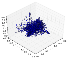
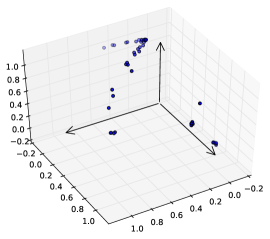
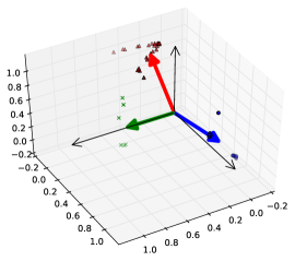
(a)(b)(c)

Figure 1: An execution of Algorithm 1 under the Gaussian Covariates model, for $d=3$, $n=m_{0}=5000$, the standard basis as parameter vectors, and uniform weights, using $\xi_{0}=2\sqrt{d}$. The $m$ pre-candidate vectors ${\boldsymbol{w}}({\boldsymbol{\xi}})$ are shown in subfigure (a) as points. Subfigure (b) contains the top 50 vectors with highest norm, after they have been normalized. These vectors are clustered using $k$-means in subfigure (c), and the resulting cluster centers are indicated with thick arrows.

4 Main Results

4.1 Generic Combinations under Value Oracle and Gaussian Covariates Models

Our first result establishes that Algorithm 1 indeed produces candidates clustered around $\{{\boldsymbol{w}}^{\ell}\}_{\ell=1}^{k}$:

Theorem 1.

Let $\{{\boldsymbol{\tilde{w}}}(\xi^{1}),\dots,{\boldsymbol{\tilde{w}}}(\xi^{m})\}$, where $m\leq m_{0}$, be the output of the CandidateGeneration algorithm. Then, for any $\delta\in(0,0.5]$, and any $\rho\in(0,1)$, there exist $w_{0}=\Theta\left(\frac{\delta u_{0}^{2}}{k}\right)$, $\xi_{0}=\Theta\left(\frac{k^{2}}{\kappa\beta\rho}\log\frac{k}{u_{0}\delta}\right)$, $\gamma=\Theta(\frac{\kappa\rho}{k^{2}})$, for which the following occur with probability at least $1-\delta$: the set of candidate indices ${\mathcal{C}}\subseteq[m_{0}]$ can be partitioned as ${\mathcal{C}}={\mathcal{C}}_{0}\cup{\mathcal{C}}_{1}\cup\cdots\cup{\mathcal{C}}_{k}\,$ so that if $i\in{\mathcal{C}}_{\ell}$ then $\big{\|}{\boldsymbol{\tilde{w}}}({\boldsymbol{\xi}}^{i})-{\boldsymbol{w}}^{\ell}\big{\|}_{2}\leq 6\delta\,,$ and $|{\mathcal{C}}_{\ell}|\geq\gamma m_{0}/2$, for all $\ell\in[k]$, while ${\mathcal{C}}_{0}$ is a set of ‘bad’ candidates such that $|{\mathcal{C}}_{0}|\leq 2\rho\gamma m_{0}$. This occurs for (a) $m_{0}>C\frac{1}{\gamma\rho}\log\frac{k}{\delta}\,,$ and (b) either $n_{0}>C^{\prime}\frac{dM^{2}}{\delta^{2}w_{0}^{2}}\log\frac{k}{\gamma\rho\delta}\,,$ under the Value Oracle model, or $n>\frac{M^{4}d^{2}}{\delta^{2}w_{0}^{2}}\max\left(C^{\prime\prime}\Big{(}\frac{k}{\gamma\rho\delta}\right)^{1+7(1+2d^{-1})\xi_{0}^{2}},e^{4d\left(\frac{1}{7}+(1+2d^{-1})\xi_{0}^{2}\right)}\Big{)}\,,$ under the Gaussian Covariates model, for some absolute constants $C,C^{\prime},C^{\prime\prime}$.

There are several observations to be made. First, the gradient estimation procedures outlined in 3.3 indeed yield sufficiently accurate estimates so that, asymptotically, the candidates ${\boldsymbol{w}}^{\ell}$ concentrate around the parameter vectors. On the other hand, there exists also a set of ‘bad’ candidates, that may not necessarily be close to any parameter vector. However, this set can be made arbitrarily small compared to the smallest set of ‘valid’ candidates: indeed, for any $\rho\in(0,1)$, choosing $m_{0}$ and $n_{0}$ or $n$ as in the theorem yields $|{\mathcal{C}}_{0}|/\min_{\ell}|{\mathcal{C}}_{\ell}|\leq 4\rho$. The spurious set ${\mathcal{C}}_{0}$ is unavoidable; beyond incorrect estimates the gradient (occurring with low probability as $n_{0}$ and $n$ increases), if $d>2$, there are also ${\boldsymbol{\xi}}$s that are approximately normal to more than one parameter vectors ${\boldsymbol{w}}^{\ell}$, $\ell\in[k]$. Nonetheless, this is significantly less likely than the event that ${\boldsymbol{\xi}}$ is approximately normal to (and thus, estimating) only one of the parameter vectors (c.f. Lemma 5.4).

In both gradient estimation models, a small ($m_{0}=\Theta(\log k)$) number of ${\boldsymbol{\xi}}$s suffices to correctly estimate the clusters. On the other hand, the sample complexity scales as $n=m_{0}\times n_{0}=\Theta(d\log k)$ in the Value Oracle model, and $n=e^{\Theta(d\cdot\mathtt{poly}(k))}$ in the Gaussian Covariates model. Nevertheless, in the next section, we show that the exponential dependence on $d$ can be avoided when $k\ll d$.

4.2 Gaussian Covariates with Dimensionality Reduction

We avoid the exponential dependence on $d$ under Gaussian Covariates by preprocessing covariates through a dimensionality reduction method. Observe that $r({\boldsymbol{x}})$ depends on ${\boldsymbol{x}}$ only through the $k$ inner products $\langle{\boldsymbol{w}}^{\ell},{\boldsymbol{x}}\rangle$, $\ell\in[k]$. As a result, projecting a ${\boldsymbol{x}}^{(i)}$ to the $k$-dimensional linear space spanned by $\{{\boldsymbol{w}}^{\ell}\}_{\ell=1}^{k}$ and estimating the gradient would result in no loss of information. Most importantly, this eliminates the dependence of the gradient estimation on $d$. Discovering the linear span of $\{{\boldsymbol{w}}^{\ell}\}_{\ell=1}^{k}$ can be performed using, e.g., the SpectralMirror method of Sun et al. (2014) in the mixture case:

Theorem 2 (Sun et al. (2014)).

Given $n$ covariate/label pairs generated through the Gaussian Covariates model in the mixture case, the SpectralMirror Algorithm constructs an estimate $\hat{\mathcal{M}}$ of $\mathcal{M}=\operatorname{span}({\boldsymbol{M}})$ s.t., for all $\theta\leq u_{0}\kappa$, the largest principal angle $d_{P}$ between $\mathcal{M}$ and $\hat{\mathcal{M}}$ satisfies ${\mathbb{P}}\{d_{P}(\mathcal{M},\hat{\mathcal{M}})>\theta\}\leq C_{1}e^{-C_{2}\frac{n\theta^{2}}{d}}.$ with $C_{1}$, $C_{2}$ absolute constants.

The above theorem is a special case of Theorem 1 of (Sun et al., 2014), when the covariates are sampled from a standard (rather than arbitrary) Gaussian. In short, it implies that $O(\frac{d}{\theta^{2}})$ points suffice to produce a linear space within a $\theta$ angle from $\mathcal{M}=\operatorname{span}({\boldsymbol{M}})$. We leverage this result to improve on the bound of Theorem 1 for Gaussian covariates. First, given $n$ samples from the Gaussian Covariates model, we use as subset of these samples to produce an estimate $\hat{\mathcal{M}}$ of $\mathcal{M}$ through the SpectralMirror algorithm. To estimate the gradient $\nabla r({\boldsymbol{\xi}})$ at ${\boldsymbol{\xi}}\in{\mathbb{R}}^{d}$ using the remaining samples, we apply again (4) on the projections of ${\boldsymbol{x}}^{(i)}$ to $\hat{\mathcal{M}}.$ More formally:

• Gradient Estimation with Projected Gaussian Covariates. Use $n_{1}<n$ samples to produce an estimate $\hat{\mathcal{M}}$ of $\mathcal{M}$. For every ${\boldsymbol{x}}\in{\mathbb{R}}^{d}$, denote by ${\boldsymbol{\hat{x}}}$ the projection of ${\boldsymbol{x}}$ to $\hat{\mathcal{M}}$. Using the remaining $n_{2}=n-n_{1}$ samples, the estimate of $\nabla r({\boldsymbol{\xi}})$ at ${\boldsymbol{\xi}}\in{\mathbb{R}}^{s}$ is given by:

  $${\boldsymbol{w}}({\boldsymbol{\xi}})\equiv\frac{\sum_{i=n_{1}+1}^{n}K({\boldsymbol{\xi}},{\boldsymbol{\hat{x}}}^{(i)})\,y^{(i)}\big{(}{\boldsymbol{\hat{x}}}^{(i)}-{\boldsymbol{\hat{x}}}({\boldsymbol{\xi}})\big{)}}{\sum_{i=n_{1}+1}^{n}K({\boldsymbol{\xi}},{\boldsymbol{\hat{x}}}^{(i)})},$$ (5)

  where $K({\boldsymbol{\xi}},{\boldsymbol{x}})=e^{\langle{\boldsymbol{\xi}},{\boldsymbol{x}}\rangle}$ and ${\boldsymbol{\hat{x}}}({\boldsymbol{\xi}})\equiv\frac{\sum_{i=n_{1}+1}^{n}K({\boldsymbol{\xi}},{\boldsymbol{\hat{x}}}^{(i)})\,{\boldsymbol{\hat{x}}}^{(i)}}{\sum_{i=n_{1}+1}^{n}K({\boldsymbol{\xi}},{\boldsymbol{\hat{x}}}^{(i)})}.$

Note that ${\boldsymbol{w}}({\boldsymbol{\xi}})={\boldsymbol{w}}({\boldsymbol{\hat{\xi}}})$, i.e., the estimate depends on ${\boldsymbol{\xi}}$ only through its projection to $\hat{\mathcal{M}}$. The estimation (5) replaces (4) in Algorithm 1, indeed eliminating the exponential dependence on $d$:

Theorem 3.

Let $\{{\boldsymbol{\tilde{w}}}(\xi^{1}),\dots,{\boldsymbol{\tilde{w}}}(\xi^{m})\}$, where $m\leq m_{0}$, be the output of the CandidateGeneration algorithm when (5) is used to produce ${\boldsymbol{w}}({\boldsymbol{\xi}})$ in the mixture case. Then, for any $\delta\in(0,0.5]$, and any $\rho\in(0,1)$, there exist $w_{0}=\Theta\left(\frac{\delta u_{0}^{2}}{k}\right)$, $\xi_{0}=\Theta\left(\frac{k^{2}}{\kappa\beta\rho}\log\frac{k}{u_{0}\delta}\right)$, $\gamma=\Theta(\frac{\kappa\rho}{k^{2}})$, for which the following occurs with probability at least $1-\delta$: the set of candidate indices ${\mathcal{C}}\subseteq[m_{0}]$, can be partitioned as ${\mathcal{C}}={\mathcal{C}}_{0}\cup{\mathcal{C}}_{1}\cup\cdots\cup{\mathcal{C}}_{k}\,,$ so that if $i\in{\mathcal{C}}_{\ell}$ then $\big{\|}{\boldsymbol{\tilde{w}}}({\boldsymbol{\xi}}^{i})-{\boldsymbol{w}}^{\ell}\big{\|}_{2}\leq 7\delta\,,$ and $|{\mathcal{C}}_{\ell}|\geq\gamma m_{0}/2$, for all $\ell\in[k]$, while ${\mathcal{C}}_{0}$ is a set of ‘bad’ candidates such that $|{\mathcal{C}}_{0}|\leq 2\rho\gamma m_{0}$. This occurs for (a) $m_{0}>C\frac{1}{\gamma\rho}\log\frac{k}{\delta}\,,$ and (b) $n_{1}>C^{\prime}d\left(\min\left\{2\arcsin\frac{\sqrt{3}\kappa}{8k},2\arcsin\frac{\delta^{2}}{4k},u_{0}\kappa\right\}\right)^{-1}$ and $n_{2}>\frac{M^{4}k^{2}}{\delta^{2}w_{0}^{2}}\max\left(C^{\prime\prime}\left(\frac{k}{\gamma\rho\delta}\right)^{1+7(1+2k^{-1})\xi_{0}^{2}},e^{4k\left(\frac{1}{7}+(1+2k^{-1})\xi_{0}^{2}\right)}\right),$ for absolute constants $C,C^{\prime},C^{\prime\prime}$.

Hence, $n_{1}=\Theta(dk)$ suffices to estimate $\mathcal{M}$, while $n_{2}=e^{\Theta(k^{5}\log^{2}k)}$ suffices for gradient estimation.

5 Proof of Theorem 1

We prove Theorem 1 below. The proofs of all lemmas, as well as the proof of Theorem 3, can be found in the appendix.

5.1 Concentration Results

We first establish some concentration results regarding gradient estimation through (3) and (4). For ${\boldsymbol{\xi}}\in{\mathbb{R}}^{d}$, let ${\mathbb{E}}_{\boldsymbol{\xi}}\{\cdot\}$ be the expectation with respect to a Gaussian random variable ${\boldsymbol{X}}\sim{\sf N}({\boldsymbol{\xi}},{\rm I}_{d\times d})$ centered at ${\boldsymbol{\xi}}$, and let:

$${\boldsymbol{\overline{w}}}({\boldsymbol{\xi}})={\mathbb{E}}_{\boldsymbol{\xi}}\big{\{}\nabla r({\boldsymbol{X}})\big{\}}=\textstyle\sum_{\ell=1}^{k}u_{\ell}{\boldsymbol{w}}^{\ell}{\mathbb{E}}_{{\boldsymbol{\xi}}}\big{\{}f^{\prime}\big{(}\langle{\boldsymbol{w}}^{\ell},{\boldsymbol{X}}\rangle\big{)}\big{\}}\,.$$ (6)

Given ${\boldsymbol{\xi}}\in{\mathbb{R}}^{d}$, (6) is the expectation of estimate ${\boldsymbol{w}}({\boldsymbol{\xi}})$, under both (3) and (4): this is a consequence of Stein’s lemma Stein (1973). We also characterize the rate of convergence of ${\boldsymbol{w}}({\boldsymbol{\xi}})$ to ${\boldsymbol{\overline{w}}}({\boldsymbol{\xi}})$:

Lemma 5.1 (Value Oracle Concentration Bound).

There exist numerical constants $c_{1},c_{2},c_{2},$ and $c_{4}$ such that, when ${\boldsymbol{w}}({\boldsymbol{\xi}})$ is computed through (3), for any fixed ${\boldsymbol{\xi}}\in{\mathbb{R}}^{d}$:

$${\mathbb{P}}\Big{\{}\big{\|}{\boldsymbol{w}}({\boldsymbol{\xi}})-{\boldsymbol{\overline{w}}}({\boldsymbol{\xi}})\big{\|}_{2}\geq\delta\Big{\}} \leq c_{1}\exp\Big{(}-\min\big{\{}\frac{c_{2}n_{0}\delta^{2}}{dM^{2}},(c_{3}\frac{\sqrt{n_{0}}\delta}{M}-c_{4}\sqrt{d})^{2}\big{\}}\Big{)}\,.$$ (7)

The proof of this lemma can be found in Appendix A, and relies on the sub-gaussianity of the r.v. $y{\boldsymbol{x}}$, when ${\boldsymbol{x}}$ is gaussian and $y$ is given by (1). Similarly, under the Gaussian Covariates model:

Lemma 5.2 (Gaussian Covariates Concentration Bound).

There exists a numerical constant $C$ such that, when ${\boldsymbol{w}}({\boldsymbol{\xi}})$ is computed through (4), for any fixed ${\boldsymbol{\xi}}\in{\mathbb{R}}^{d}$:

$${\mathbb{P}}\Big{\{}\big{\|}{\boldsymbol{w}}({\boldsymbol{\xi}})-{\boldsymbol{\overline{w}}}({\boldsymbol{\xi}})\big{\|}_{2}\geq\delta\Big{\}} \leq\frac{Ce^{\|{\boldsymbol{\xi}}\|_{2}^{2}}}{n\delta^{2}}\,M^{4}(d+\|{\boldsymbol{\xi}}\|^{2})^{2}\,.$$ (8)

The proof of this lemma can also be found in Appendix A.

5.2 Characterizing Gradient Coefficients and Approximate Normality

Eq. (6) indicates that, asymptotically, ${\boldsymbol{\overline{w}}}({\boldsymbol{\xi}})$ is a linear combination of the vectors ${\boldsymbol{w}}^{\ell}$. The following lemma, proved in Appendix B.1, bounds the coefficients of this linear combination:

Lemma 5.3.

For any $\ell\in[k]$ and ${\boldsymbol{\xi}}\in{\mathbb{R}}^{d}$,

$$\beta\Phi(-2\beta)\,e^{-2\beta|\langle{\boldsymbol{w}}^{\ell},{\boldsymbol{\xi}}\rangle|+2\beta^{2}}\leq{\mathbb{E}}_{{\boldsymbol{\xi}}}\big{\{}f^{\prime}\big{(}\langle{\boldsymbol{w}}^{\ell},{\boldsymbol{X}}\rangle\big{)}\big{\}}\leq{8}{\beta}e^{-2\beta|\langle{\boldsymbol{w}}^{\ell},{\boldsymbol{\xi}}\rangle|+2{\beta^{2}}}\,,$$ (9)

where $\Phi(x)=\int_{-\infty}^{x}e^{-z^{2}/2}{\rm d}z/\sqrt{2\pi}$ is the one-dimensional Gaussian distribution function, and ${\mathbb{E}}_{\boldsymbol{\xi}}$ is the expectation with respect to a Gaussian random variable ${\boldsymbol{X}}\sim{\sf N}({\boldsymbol{\xi}},{\rm I}_{d\times d})$ centered at ${\boldsymbol{\xi}}$.

The lemma implies that a vector ${\boldsymbol{w}}^{\ell}$ contributes significantly to ${\boldsymbol{\overline{w}}}({\boldsymbol{\xi}})$ only if $z_{\ell}=\langle{\boldsymbol{w}}^{\ell},{\boldsymbol{\xi}}\rangle\simeq 0$, and ${\boldsymbol{\xi}}$ is approximately normal to ${\boldsymbol{w}}^{\ell}$. Thus, if ${\boldsymbol{\xi}}$ is approximately normal to only one ${\boldsymbol{w}}^{\ell}$, ${\boldsymbol{w}}({\boldsymbol{\xi}})\approx{\boldsymbol{w}}^{\ell}$. Clearly, the success of the candidate generation process depends on the event that a randomly generated ${\boldsymbol{\xi}}$ is on approximately normal to a single parameter vector, but not two. The following lemma, whose proof can be found in Appendix B.2, bounds the probabilities of these events:

Lemma 5.4.

Assume that ${\boldsymbol{\Xi}}\in{\mathbb{R}}^{d}$ is sampled from ${\sf N}(0,\xi_{0}^{2}\,{\rm I}_{d})$. Then, for any $0<\Delta<\xi_{0}$, ${\mathbb{P}}(|\langle{\boldsymbol{w}}^{\ell},{\boldsymbol{\Xi}}\rangle|<\Delta)\geq\sqrt{\frac{2}{e\pi}}\frac{\Delta}{\xi_{0}},$ for all $\ell\in[k]$ and for any $\Delta_{1},\Delta_{2}>0$, ${\mathbb{P}}(|\langle{\boldsymbol{w}}^{\ell},{\boldsymbol{\Xi}}\rangle|<\Delta_{1},|\langle{\boldsymbol{w}}^{\ell^{\prime}},{\boldsymbol{\Xi}}\rangle|<\Delta_{2})\leq\frac{2\Delta_{1}\Delta_{2}}{\pi\kappa\xi_{0}^{2}}$, for all $\ell,\ell^{\prime}\in[k]$ with $\ell\neq\ell^{\prime}$.

5.3 Candidate Partitioning

We now describe how the $m$ candidate indices ${\mathcal{C}}\subset[m_{0}]$ produced by Algorithm 1 can be partitioned as ${\mathcal{C}}={\mathcal{C}}_{0}\cup{\mathcal{C}}_{1}\cup\cdots\cup{\mathcal{C}}_{k}\,,$ s.t. for any $i\in{\mathcal{C}}_{\ell}$, candidate ${\boldsymbol{\tilde{w}}}({\boldsymbol{\xi}}^{(i)})$ is close to ${\boldsymbol{w}}^{\ell}$, while ${\mathcal{C}}_{0}$ is a small set of spurious candidates. Let $c_{1}=c_{1}(\beta)\equiv\beta\Phi(-2\beta)e^{2\beta^{2}}$ and $c_{2}=c_{2}(\beta)\equiv 8\beta e^{2\beta^{2}}$, where $\Phi$ as in Lemma 5.3. Given $\delta\in(0,0.5],$ and $\rho\in(0,1)$, let

$$\Delta=\ \frac{1}{\beta}\log\frac{(1+\delta)c_{2}k}{c_{1}u_{0}\delta},$$ (10)

and set the parameters of Algorithm 1 as follows

$$w_{0} \equiv\frac{1}{\delta}kc_{2}e^{-2\beta\Delta}=\frac{c_{1}^{2}u_{0}^{2}\delta}{(1+\delta)^{2}c_{2}k},$$ (11)

$$\xi_{0} \equiv 2\sqrt{\frac{2e}{\pi}}\frac{k}{\kappa}(\frac{k}{\rho}+1)\Delta=\frac{2}{\beta}\sqrt{\frac{2e}{\pi}}\frac{k}{\kappa}(\frac{k}{\rho}+1)\log\frac{(1+\delta)c_{2}k}{c_{1}u_{0}\delta},\quad\text{and}$$ (12)

$$\gamma \equiv\sqrt{\frac{1}{2e\pi}}\frac{\Delta}{\xi_{0}}-\frac{2k}{\kappa\pi}\left(\frac{\Delta}{\xi_{0}}\right)^{2}=\frac{\kappa\rho}{4e(\rho+\kappa)^{2}}$$ (13)

Note that our choice of $\xi_{0}$ is such that $\frac{\Delta}{\xi_{0}}$ satisfies the equation:

$$\frac{2k^{2}}{\pi\kappa}\left(\frac{\Delta}{\xi_{0}}\right)^{2}=\rho\cdot\left(\sqrt{\frac{1}{2e\pi}}\frac{\Delta}{\xi_{0}}-\frac{2k}{\kappa\pi}\left(\frac{\Delta}{\xi_{0}}\right)^{2}\right)=\rho\gamma.$$ (14)

We define the following partition of ${\mathbb{R}}^{d}={\mathcal{R}}_{0}\bigcup\Big{\{}\bigcup_{\ell=1}^{k}{\mathcal{R}}_{\ell}\Big{\}}\cup{\mathcal{R}}_{*}\,,$:

$${\mathcal{R}}_{0} \equiv\big{\{}{\boldsymbol{\xi}}\in{\mathbb{R}}^{d}:\,\min_{i\in[k]}|\langle{\boldsymbol{w}}^{i},{\boldsymbol{\xi}}\rangle|\geq\Delta\big{\}}\,,$$ (15a)

$${\mathcal{R}}_{\ell} \equiv\big{\{}{\boldsymbol{\xi}}\in{\mathbb{R}}^{d}:\,\,|\langle{\boldsymbol{w}}^{\ell},{\boldsymbol{\xi}}\rangle|<\Delta,\;\min_{i\in[k]\setminus\ell}|\langle{\boldsymbol{w}}^{i},{\boldsymbol{\xi}}\rangle|\geq\Delta\big{\}}\,,$$ (15b)

$${\mathcal{R}}_{*} \equiv\big{\{}{\boldsymbol{\xi}}\in{\mathbb{R}}^{d}:\,\,\exists\ell_{1},\ell_{2}\in[k]:\;\ell_{1}\neq\ell_{2},\;|\langle{\boldsymbol{w}}^{\ell_{1}},{\boldsymbol{\xi}}\rangle|<\Delta,\;|\langle{\boldsymbol{w}}^{\ell_{2}},{\boldsymbol{\xi}}\rangle|<\Delta\big{\}}\,.$$ (15c)

By (6) and (9), for ${\boldsymbol{\xi}}\in{\mathcal{R}}_{0}$, ${\boldsymbol{\overline{w}}}({\boldsymbol{\xi}})$ can be rewritten as ${\boldsymbol{\overline{w}}}({\boldsymbol{\xi}})={\boldsymbol{M}}{\boldsymbol{v}}$, where $\|{\boldsymbol{v}}\|_{2}\leq\sqrt{k}c_{2}e^{-2\beta\Delta}$. Hence, as $\|{\boldsymbol{M}}\|_{2}\leq\|{\boldsymbol{M}}\|_{F}=\sqrt{k}$, for any ${\boldsymbol{\xi}}\in{\mathcal{R}}_{0}$,

$$\|{\boldsymbol{\overline{w}}}({\boldsymbol{\xi}})\|_{2}\leq k\,c_{2}\,e^{-2\beta\Delta}\stackrel{{\scriptstyle\eqref{w0}}}{{=}}\delta w_{0}\,.$$ (16)

Similarly, the sets ${\mathcal{R}}_{\ell}$ are such that for any ${\boldsymbol{\xi}}\in{\mathcal{R}}_{\ell}$

$$\|{\boldsymbol{\overline{w}}}({\boldsymbol{\xi}})-a_{\ell}{\boldsymbol{w}}^{\ell}\|_{2}\leq k\,c_{2}\,e^{-2\beta\Delta}=\delta w_{0}\,,$$ (17)

where $a_{\ell}\equiv|u_{\ell}|\cdot{\mathbb{E}}_{0}\Big{\{}f^{\prime}\big{(}\langle{\boldsymbol{w}}^{\ell},\xi+{\boldsymbol{X}}\rangle\big{)}\Big{\}}$. This follows from the same argument used above in proving (16). Moreover, from Eq. (9):

$$c_{1}u_{0}e^{-2\beta\Delta}\leq|a_{\ell}|=|u_{\ell}|\cdot{\mathbb{E}}_{0}\Big{\{}f^{\prime}\big{(}\langle{\boldsymbol{w}}^{\ell},\xi+{\boldsymbol{X}}\rangle\big{)}\Big{\}}\leq c_{2}\,.$$ (18)

Armed with the above observations, we partition the set of generated ${\boldsymbol{\xi}}$’s as $[m_{0}]\equiv{\mathcal{G}}\cup{\mathcal{G}}^{c}$, where ${\mathcal{G}}\equiv\Big{\{}j\in[m_{0}]:\,\|{\boldsymbol{w}}({\boldsymbol{\xi}}_{j})-{\boldsymbol{\overline{w}}}({\boldsymbol{\xi}}_{j})\|_{2}\leq\delta w_{0}\Big{\}}\,.$ Recall that the candidate set is, by construction, ${\mathcal{C}}\equiv\Big{\{}j\in[m_{0}]:\,\|{\boldsymbol{w}}({\boldsymbol{\xi}}_{j})\|_{2}\geq w_{0}\}$. We define the partition of the candidate set, as described in Theorem 1, as follows: for each $\ell\in[k]$, let ${\mathcal{C}}_{\ell}\equiv\Big{\{}j\in{\mathcal{G}}:\,{\boldsymbol{\xi}}_{j}\in{\mathcal{R}}_{\ell},\;\|{\boldsymbol{w}}({\boldsymbol{\xi}}_{j})\|_{2}\geq w_{0}\Big{\}}\,,$ and ${\mathcal{C}}_{0}\equiv\Big{\{}j\in[m_{0}]:\,\|{\boldsymbol{w}}({\boldsymbol{\xi}}_{j})\|_{2}\geq w_{0}\,,j\not\in\cup_{\ell=1}^{k}{\mathcal{C}}_{\ell}\Big{\}}\,.$ Observe that this is indeed a partition of ${\mathcal{C}}$. The following lemma, whose proof can be found in Appendix C.1, establishes that candidates in the sets ${\mathcal{C}}_{\ell}$ have the desirable property stated in Thm. 1, namely, that they are clustered around the corresponding vectors $w_{\ell}$:

Lemma 5.5.

For each $\ell\in[k]$ and each $j\in{\mathcal{C}}_{\ell}$, $\big{\|}{\boldsymbol{\tilde{w}}}({\boldsymbol{\xi}}_{j})-{\boldsymbol{w}}^{\ell}\big{\|}_{2}\leq 6\delta$.

To conclude the proof, we need to show that, w.h.p., the sets ${\mathcal{C}}_{\ell}$ are large, while the spurious set ${\mathcal{C}}_{0}$ is small. The next lemma upper-bounds the size of the spurious candidate set $C_{0}$:

Lemma 5.6.

The event $|{\mathcal{C}}_{0}|\leq 2\gamma\rho m_{0}$ occurs with probability at least (b) $1-\Big{[}\frac{c_{1}}{\gamma\rho}\exp\Big{(}-\min\big{\{}\frac{c_{2}n_{0}\delta^{2}w_{0}^{2}}{dM^{2}},(c_{3}\frac{\sqrt{n_{0}}\delta w_{0}}{M}-c_{4}\sqrt{d})^{2}\big{\}}\Big{)}+e^{-c_{5}m_{0}\gamma\rho}\Big{]}$, with $c_{1},\ldots,c_{5}$ absolute constants, under the Value Oracle model, and (b) $1-\Big{(}\frac{c_{1}}{\gamma\rho}\left(\frac{M^{4}d^{2}}{n\delta^{2}w_{0}^{2}}\right)^{\frac{1}{1+4(1+2d^{-1})\xi_{0}^{2}}}+e^{-c_{2}m_{0}\gamma\rho}\Big{)}$, for $n>\frac{M^{4}d^{2}}{\delta^{2}w_{0}^{2}}e^{4d\left(\frac{1}{7}+(1+2d^{-1})\xi_{0}^{2}\right)}$ and $c_{1},c_{2}$ absolute constants, under the Gaussian Covariates model.

The proof can be found in Appendix C.2. The next lemma, whose proof is in Appendix C.3 lower-bounds the size of sets ${\mathcal{C}}_{\ell}$:

Lemma 5.7.

For $\ell\in[k]$, the event $|{\mathcal{C}}_{\ell}|\geq m_{0}\gamma/2$ occurs with probability at least (a) $1-\Big{[}\frac{c_{1}}{\gamma\rho}\exp\Big{(}-\min\big{\{}\frac{c_{2}n_{0}\delta^{2}w_{0}^{2}}{dM^{2}},(c_{3}\frac{\sqrt{n_{0}}\delta w_{0}}{M}-c_{4}\sqrt{d})^{2}\big{\}}\Big{)}+e^{-c_{5}m_{0}\gamma}\Big{]}$, where $c_{1},\ldots,c_{5}$ are absolute constants, under the Value Oracle model, and (b) $1-\left(\frac{c_{1}}{\gamma\rho}\left(\frac{M^{4}d^{2}}{n\delta^{2}w_{0}^{2}}\right)^{\frac{1}{1+7(1+2d^{-1})\xi_{0}^{2}}}+e^{-c_{3}m_{0}\gamma}\right)$, where $c_{1},c_{2}$ are absolute constants, for $n>\frac{M^{4}d^{2}}{\delta^{2}w_{0}^{2}}e^{4d\left(\frac{1}{7}+(1+2d^{-1})\xi_{0}^{2}\right)}$, under the Gaussian Covariates model.

Using the above three lemmas and by applying a union bound, we get that the events in the theorem occur with probability at least $1-\delta$ if $m_{0}>C\frac{1}{\gamma\rho}\log\frac{k}{\delta}$ and, for the Value Oracle model, $n_{0}>C^{\prime}\frac{dM^{2}}{\delta^{2}w_{0}^{2}}\log\frac{k}{\gamma\rho\delta},$ or, for the Gaussian Covariates model, $n>\frac{M^{4}d^{2}}{\delta^{2}w_{0}^{2}}\max\left(C^{\prime\prime}\left(\frac{k}{\gamma\rho\delta}\right)^{1+7(1+2d^{-1})\xi_{0}^{2}},e^{4d\left(\frac{1}{7}+(1+2d^{-1})\xi_{0}^{2}\right)}\right),$ where $C$,$C^{\prime}$, and $C^{\prime\prime}$ are absolute constants.∎

Appendix A Proof of Concentration Results

A.1 Proof of Lemma 5.1

We use the following variant of Stein’s identity (see Stein [1973], and Liu [1994] for this specific formulation). Let ${\boldsymbol{X}}\in{\mathbb{R}}^{d}$, ${\boldsymbol{X}}^{\prime}\in{\mathbb{R}}^{d^{\prime}}$ be jointly Gaussian random vectors, sampled from a Gaussian distribution of arbitrary mean and covariance. Consider a function $h:{\mathbb{R}}^{d^{\prime}}\to{\mathbb{R}}$ that is almost everywhere (a.e.) differentiable and satisfies ${\mathbb{E}}[|\partial h({\boldsymbol{X}}^{\prime})/\partial x_{i}|]<\infty$, for all $i\in[d^{\prime}]$. Then, the following identity holds:

$$\mathtt{Cov}({\boldsymbol{X}},h({\boldsymbol{X}}^{\prime}))=\mathtt{Cov}({\boldsymbol{X}},{\boldsymbol{X}}^{\prime}){\mathbb{E}}[\nabla h({\boldsymbol{X}}^{\prime})].$$ (19)

Observe first that for ${\boldsymbol{X}}$ a Gaussian vector centered at ${\boldsymbol{\xi}}$:

$$\mathtt{Cov}({\boldsymbol{X}},r({\boldsymbol{X}})) \equiv{\mathbb{E}}_{{\boldsymbol{\xi}}}\left[({\boldsymbol{X}}-{\mathbb{E}}[{\boldsymbol{X}}])(r({\boldsymbol{X}})-{\mathbb{E}}[r({\boldsymbol{X}})])\right]={\mathbb{E}}_{\boldsymbol{\xi}}\left[({\boldsymbol{X}}-{\mathbb{E}}[{\boldsymbol{X}}])r({\boldsymbol{X}})\right]$$

$$={\mathbb{E}}_{\boldsymbol{\xi}}\left[({\boldsymbol{X}}-{\boldsymbol{\xi}})r({\boldsymbol{X}})\right].$$ (20)

Thus, in the case of the Value Oracle model, we have that:

$${\mathbb{E}}[{\boldsymbol{w}}({\boldsymbol{x}})] \stackrel{{\scriptstyle\eqref{voestimate}}}{{=}}{\mathbb{E}}_{{\boldsymbol{\xi}}}[({\boldsymbol{X}}-{\boldsymbol{\xi}})r({\boldsymbol{X}})]\stackrel{{\scriptstyle\eqref{dropmean}}}{{=}}\mathtt{Cov}({\boldsymbol{X}},r({\boldsymbol{X}}))$$

$$\stackrel{{\scriptstyle\eqref{stein}}}{{=}}\mathtt{Cov}({\boldsymbol{X}},{\boldsymbol{X}}){\mathbb{E}}_{{\boldsymbol{\xi}}}[\nabla r({\boldsymbol{X}})]={\mathbb{E}}_{{\boldsymbol{\xi}}}[\nabla r({\boldsymbol{X}})]\equiv{\boldsymbol{\overline{w}}}({\boldsymbol{\xi}}).$$

Thus, ${\boldsymbol{w}}({\boldsymbol{\xi}})$ indeed concentrates around ${\boldsymbol{\overline{w}}}({\boldsymbol{\xi}})$ by the law of large numbers. The tail bounds in Lemma 5.1 then follow from Lemma 1 of Sun et al. [2014]. ∎

A.2 Proof of Lemma 5.2

It is convenient to define the following quantities $z({\boldsymbol{\xi}})\equiv\sum_{i=1}^{n}K({\boldsymbol{\xi}},{\boldsymbol{x}}^{(i)})\,,$ ${\boldsymbol{u}}({\boldsymbol{\xi}})\equiv\sum_{i=1}^{n}K({\boldsymbol{\xi}},{\boldsymbol{x}}^{(i)})\,{\boldsymbol{x}}^{(i)}\,,$ $s({\boldsymbol{\xi}})\equiv\sum_{i=1}^{n}K({\boldsymbol{\xi}},{\boldsymbol{x}}^{(i)})\,y^{(i)}\,,$ and ${\boldsymbol{v}}({\boldsymbol{\xi}})\equiv\sum_{i=1}^{n}K({\boldsymbol{\xi}},{\boldsymbol{x}}^{(i)})\,y^{(i)}{\boldsymbol{x}}^{(i)}\,.$ Note that, in terms of these quantities, we have ${\boldsymbol{w}}({\boldsymbol{\xi}})=\frac{{\boldsymbol{v}}({\boldsymbol{\xi}})}{z({\boldsymbol{\xi}})}-\frac{{\boldsymbol{u}}({\boldsymbol{\xi}})\,s({\boldsymbol{\xi}})}{z({\boldsymbol{\xi}})^{2}}\,.$ The following concentration results then hold:

Lemma A.1.

For any fixed ${\boldsymbol{\xi}}\in{\mathbb{R}}^{d}$, let ${\mathbb{E}}_{{\boldsymbol{\xi}}}\{\cdots\}$ denote the expectation with respect to ${\boldsymbol{X}}\sim{\sf N}({\boldsymbol{\xi}},{\rm I}_{d})$. Then, if $\{x^{(i)}\}_{i=1,\ldots,n}$ are generated under the Gaussian covariates model, we have

$${\mathbb{E}}\,z({\boldsymbol{\xi}}) =n\,e^{\|{\boldsymbol{\xi}}\|_{2}^{2}/2}\,, {\mathbb{E}}\,{\boldsymbol{u}}({\boldsymbol{\xi}}) =n\,e^{\|{\boldsymbol{\xi}}\|_{2}^{2}/2}\,{\mathbb{E}}_{{\boldsymbol{\xi}}}{\boldsymbol{X}}\,=n\,e^{\|{\boldsymbol{\xi}}\|_{2}^{2}/2}\,{\boldsymbol{\xi}},$$ (21a)

$${\mathbb{E}}\,s({\boldsymbol{\xi}}) =n\,e^{\|{\boldsymbol{\xi}}\|_{2}^{2}/2}\,{\mathbb{E}}_{{\boldsymbol{\xi}}}r({\boldsymbol{X}})\,, {\mathbb{E}}\,{\boldsymbol{v}}({\boldsymbol{\xi}}) =n\,e^{\|{\boldsymbol{\xi}}\|_{2}^{2}/2}\,{\mathbb{E}}_{{\boldsymbol{\xi}}}\big{\{}{\boldsymbol{X}}\,r({\boldsymbol{X}})\big{\}}\,.$$ (21b)

and

$${\mathbb{P}}\Big{\{}\big{|}z({\boldsymbol{\xi}})\!-\!{\mathbb{E}}\,z({\boldsymbol{\xi}})\big{|}\geq n\delta\Big{\}}\!\leq\!\frac{e^{2\|{\boldsymbol{\xi}}\|_{2}^{2}}}{n\delta^{2}}\,,{\mathbb{P}}\Big{\{}\big{\|}{\boldsymbol{u}}({\boldsymbol{\xi}})\!-\!{\mathbb{E}}\,{\boldsymbol{u}}({\boldsymbol{\xi}})\big{\|}_{2}\geq n\delta\Big{\}}\!\leq\!\frac{e^{2\|{\boldsymbol{\xi}}\|_{2}^{2}}(d\!+\!4\|{\boldsymbol{\xi}}\|_{2}^{2})}{n\delta^{2}},$$ (22a)

$${\mathbb{P}}\Big{\{}\big{|}s({\boldsymbol{\xi}})\!-\!{\mathbb{E}}\,s({\boldsymbol{\xi}})\big{|}\geq n\delta\Big{\}}\!\leq\!\frac{e^{2\|{\boldsymbol{\xi}}\|_{2}^{2}}M^{2}}{n\delta^{2}}\,,{\mathbb{P}}\Big{\{}\big{\|}{\boldsymbol{v}}({\boldsymbol{\xi}})\!-\!{\mathbb{E}}\,{\boldsymbol{v}}({\boldsymbol{\xi}})\big{\|}_{2}\geq n\delta\Big{\}}\!\leq\!\frac{e^{2\|{\boldsymbol{\xi}}\|_{2}^{2}}M^{2}(d\!+\!4\|{\boldsymbol{\xi}}\|_{2}^{2})}{n\delta^{2}}.$$ (22b)

Proof.

We use the following two simple properties of Gaussian random variables. For $g:{\mathbb{R}}^{d}\to{\mathbb{R}}^{m}$, we have that for ${\boldsymbol{X}}\sim{\sf N}(0,{\rm I}_{d})$:

$${\mathbb{E}}_{0}[e^{{\boldsymbol{\xi}}^{T}{\boldsymbol{X}}}g({\boldsymbol{X}})]=e^{\|{\boldsymbol{\xi}}\|_{2}^{2}/2}{\mathbb{E}}_{{\boldsymbol{\xi}}}[g({\boldsymbol{X}})]$$ (23)

and

$${\sf{Cov}}[e^{{\boldsymbol{\xi}}^{T}{\boldsymbol{X}}}g({\boldsymbol{X}})]=e^{2\|{\boldsymbol{\xi}}\|_{2}^{2}}{\mathbb{E}}_{2{\boldsymbol{\xi}}}[g({\boldsymbol{X}})g^{T}({\boldsymbol{X}})]-e^{\|{\boldsymbol{\xi}}\|_{2}^{2}}{\mathbb{E}}_{{\boldsymbol{\xi}}}[g({\boldsymbol{X}})]{\mathbb{E}}_{{\boldsymbol{\xi}}}[g^{T}({\boldsymbol{X}})]$$ (24)

The statements in (21) therefore follow from (23) and the definition of the kernel $K$. By Chebyshev’s inequality,

$${\mathbb{P}}\Big{\{}\big{|}z({\boldsymbol{\xi}})-{\mathbb{E}}\,z({\boldsymbol{\xi}})\big{|}\geq n\delta\Big{\}}\leq\frac{{\sf{Var}}\{e^{{\boldsymbol{\xi}}^{T}{\boldsymbol{X}}}\}}{n\delta^{2}}\stackrel{{\scriptstyle\eqref{covariance}}}{{=}}\frac{e^{2\|{\boldsymbol{\xi}}\|_{2}^{2}}-e^{\|{\boldsymbol{\xi}}\|_{2}^{2}}}{n\delta^{2}}\leq\frac{e^{2\|{\boldsymbol{\xi}}\|_{2}^{2}}}{n\delta^{2}}.$$

Moreover, by Markov’s inequality:

$${\mathbb{P}}\Big{\{}\big{\|}{\boldsymbol{u}}({\boldsymbol{\xi}}) -{\mathbb{E}}\,{\boldsymbol{u}}({\boldsymbol{\xi}})\big{\|}_{2}\geq n\delta\Big{\}}\leq\frac{{\mathbb{E}}\big{\|}{\boldsymbol{u}}({\boldsymbol{\xi}})-{\mathbb{E}}\,{\boldsymbol{u}}({\boldsymbol{\xi}})\big{\|}_{2}^{2}}{n^{2}\delta^{2}}=\sum_{j=1}^{d}\frac{{\sf{Var}}\{{\boldsymbol{u}}_{j}({\boldsymbol{\xi}})\}}{n^{2}\delta^{2}}=\sum_{j=1}^{d}\frac{{\sf{Var}}\{e^{{\boldsymbol{\xi}}^{T}{\boldsymbol{X}}}{\boldsymbol{X}}_{j}\}}{n\delta^{2}}$$

$$\stackrel{{\scriptstyle\eqref{covariance}}}{{\leq}}\sum_{j=1}^{d}\frac{e^{2\|{\boldsymbol{\xi}}\|_{2}^{2}}{\mathbb{E}}_{2{\boldsymbol{\xi}}}[{\boldsymbol{X}}_{j}^{2}]}{n\delta^{2}}=\sum_{j=1}^{d}\frac{e^{2\|{\boldsymbol{\xi}}\|_{2}^{2}}(1+4{\boldsymbol{\xi}}_{j}^{2})}{n\delta^{2}}=\frac{e^{2\|{\boldsymbol{\xi}}\|_{2}^{2}}(d+4\|{\boldsymbol{\xi}}\|_{2}^{2})}{n\delta^{2}}$$

The first two inequalities in (22) therefore follow. The remaining two follow similarly using the fact that the absolute values of the responses $y$ are bounded by $M$. ∎

An immediate consequence of Lemma A.1 is that ${\boldsymbol{w}}({\boldsymbol{\xi}})$ concentrates around the following quantity:

$$\frac{{\mathbb{E}}{\boldsymbol{v}}({\boldsymbol{\xi}})}{{\mathbb{E}}z({\boldsymbol{\xi}})}-\frac{{\mathbb{E}}{\boldsymbol{u}}({\boldsymbol{\xi}})\,{\mathbb{E}}s({\boldsymbol{\xi}})}{\big{(}{\mathbb{E}}z({\boldsymbol{\xi}})\big{)}^{2}}\, ={\mathbb{E}}_{{\boldsymbol{\xi}}}\big{\{}{\boldsymbol{X}}\,r({\boldsymbol{X}})\big{\}}-{\mathbb{E}}_{{\boldsymbol{\xi}}}{\boldsymbol{X}}{\mathbb{E}}_{{\boldsymbol{\xi}}}r({\boldsymbol{X}})$$

$$={\sf{Cov}}_{{\boldsymbol{\xi}}}[{\boldsymbol{X}},r({\boldsymbol{X}})]\stackrel{{\scriptstyle\eqref{stein}}}{{=}}{\mathbb{E}}_{{\boldsymbol{\xi}}}[\nabla r({\boldsymbol{X}})]\equiv{\boldsymbol{\overline{w}}}({\boldsymbol{\xi}}).$$

Hence, (6) indeed describes the estimates, asymptotically. To prove (8), we use the following simple auxiliary lemma.

Lemma A.2.

For any $a,\bar{a}\in{\mathbb{R}}^{d}$, $b,\bar{b}>0$, and $\delta>0$, we have that:

$$\text{If }\|a-\bar{a}\|\leq\delta^{\prime}\text{ and }|b-\bar{b}|\leq\delta^{\prime}\text{ then }\left\|\frac{a}{b}-\frac{\bar{a}}{\bar{b}}\right\|\leq\delta$$

where

$$\delta^{\prime}=\frac{\bar{b}^{2}\delta}{(\|\bar{a}\|+\bar{b}+\bar{b}\delta)}.$$

Proof.

(Sketch) Note that $\delta^{\prime}<\bar{b}$. It is easy to show that $\left\|\frac{a}{b}-\frac{\bar{a}}{\bar{b}}\right\|\leq\frac{(\bar{b}+\|\bar{a}\|)\delta^{\prime}}{(\bar{b}-\delta^{\prime})\bar{b}}=\delta$. ∎

We have that

$${\mathbb{P}}\Big{\{}\big{\|}{\boldsymbol{w}}({\boldsymbol{\xi}})-{\boldsymbol{\overline{w}}}({\boldsymbol{\xi}})\big{\|}_{2}>\delta\Big{\}}\leq$$

$${\mathbb{P}}\Big{\{}\left\|\frac{{\boldsymbol{v}}({\boldsymbol{\xi}})}{z({\boldsymbol{\xi}})}-\frac{{\mathbb{E}}{\boldsymbol{v}}({\boldsymbol{\xi}})}{{\mathbb{E}}z({\boldsymbol{\xi}})}\right\|_{2}>\delta/2\Big{\}}+{\mathbb{P}}\Big{\{}\left\|\frac{{\boldsymbol{u}}({\boldsymbol{\xi}})s({\boldsymbol{\xi}})}{z({\boldsymbol{\xi}})^{2}}-\frac{{\mathbb{E}}{\boldsymbol{u}}({\boldsymbol{\xi}}){\mathbb{E}}s({\boldsymbol{\xi}})}{({\mathbb{E}}z({\boldsymbol{\xi}}))^{2}}\right\|_{2}>\delta/2\Big{\}}$$

From Lemma A.2, for

$$\delta^{\prime}=\frac{({\mathbb{E}}z({\boldsymbol{\xi}}))^{2}\delta}{2(\|{\mathbb{E}}{\boldsymbol{v}}({\boldsymbol{\xi}})\|_{2}+{\mathbb{E}}z({\boldsymbol{\xi}})+{\mathbb{E}}z({\boldsymbol{\xi}})\delta/2)}\stackrel{{\scriptstyle\eqref{expectations}}}{{=}}\frac{n\,e^{\|{\boldsymbol{\xi}}\|_{2}^{2}/2}}{2\|{\mathbb{E}}_{{\boldsymbol{\xi}}}{\boldsymbol{X}}r({\boldsymbol{X}})\|_{2}+2+\delta}\delta,$$ (25)

we have

$${\mathbb{P}}\Big{\{} \left\|\frac{{\boldsymbol{v}}({\boldsymbol{\xi}})}{z({\boldsymbol{\xi}})}-\frac{{\mathbb{E}}{\boldsymbol{v}}({\boldsymbol{\xi}})}{{\mathbb{E}}z({\boldsymbol{\xi}})}\right\|_{2}>\delta/2\Big{\}}\leq{\mathbb{P}}\Big{\{}\|{\boldsymbol{v}}({\boldsymbol{\xi}})-{\mathbb{E}}{\boldsymbol{v}}({\boldsymbol{\xi}})\|_{2}>\delta^{\prime}\Big{\}}+{\mathbb{P}}\Big{\{}|z({\boldsymbol{\xi}})-{\mathbb{E}}z({\boldsymbol{\xi}})|>\delta^{\prime}\Big{\}}$$

$$\stackrel{{\scriptstyle\eqref{sboundvbound},\eqref{zboundubound},\eqref{deltaprime}}}{{\leq}}\frac{M^{2}e^{2\|{\boldsymbol{\xi}}\|_{2}^{2}}(d+4\|{\boldsymbol{\xi}}\|_{2}^{2})(2\|{\mathbb{E}}_{{\boldsymbol{\xi}}}{\boldsymbol{X}}r({\boldsymbol{X}})\|_{2}+2+\delta)^{2}}{n\delta^{2}e^{\|{\boldsymbol{\xi}}\|_{2}^{2}}}+\frac{e^{2\|{\boldsymbol{\xi}}\|_{2}^{2}}(2\|{\mathbb{E}}_{{\boldsymbol{\xi}}}{\boldsymbol{X}}r({\boldsymbol{X}})\|_{2}+2+\delta)^{2}}{n\delta^{2}e^{\|{\boldsymbol{\xi}}\|_{2}^{2}}}$$

$$=\frac{\left(M^{2}(d+4\|{\boldsymbol{\xi}}\|_{2}^{2})+1\right)\left(2M\sqrt{d+\|{\boldsymbol{\xi}}\|_{2}^{2}}+2+\delta\right)^{2}e^{\|{\boldsymbol{\xi}}\|_{2}^{2}}}{n\delta^{2}},$$

where in the second to last step we use $\|{\mathbb{E}}_{{\boldsymbol{\xi}}}{\boldsymbol{X}}r({\boldsymbol{X}})\|_{2}^{2}\leq{\mathbb{E}}_{{\boldsymbol{\xi}}}\|{\boldsymbol{X}}r({\boldsymbol{X}})\|_{2}^{2}$, by the convexity of $\|\cdot\|_{2}^{2}$. Similarly, for

$$\delta^{\prime\prime} =\frac{({\mathbb{E}}z({\boldsymbol{\xi}}))^{4}\delta}{2(\|{\mathbb{E}}{\boldsymbol{u}}({\boldsymbol{\xi}})\|_{2}|{\mathbb{E}}s({\boldsymbol{\xi}})|+({\mathbb{E}}z({\boldsymbol{\xi}}))^{2}+({\mathbb{E}}z({\boldsymbol{\xi}}))^{2}\delta/2)}\stackrel{{\scriptstyle\eqref{expectations}}}{{=}}\frac{n^{2}\,e^{\|{\boldsymbol{\xi}}\|_{2}^{2}}}{2\|{\mathbb{E}}_{{\boldsymbol{\xi}}}{\boldsymbol{X}}\|_{2}|{\mathbb{E}}_{{\boldsymbol{\xi}}}r({\boldsymbol{X}})|+2+\delta}\delta,$$ (26)

we have

$${\mathbb{P}}\Big{\{}\left\|\frac{{\boldsymbol{u}}({\boldsymbol{\xi}})s({\boldsymbol{\xi}})}{z({\boldsymbol{\xi}})^{2}}-\frac{{\mathbb{E}}{\boldsymbol{u}}({\boldsymbol{\xi}}){\mathbb{E}}s({\boldsymbol{\xi}})}{({\mathbb{E}}z({\boldsymbol{\xi}}))^{2}}\right\|_{2}>\delta/2\Big{\}} \leq{\mathbb{P}}\Big{\{}\left\|{\boldsymbol{u}}({\boldsymbol{\xi}})s({\boldsymbol{\xi}})-{\mathbb{E}}{\boldsymbol{u}}({\boldsymbol{\xi}}){\mathbb{E}}s({\boldsymbol{\xi}})\right\|_{2}>\delta^{\prime\prime}\Big{\}}$$

$$\qquad+{\mathbb{P}}\Big{\{}\left|(z({\boldsymbol{\xi}}))^{2}-({\mathbb{E}}z({\boldsymbol{\xi}}))^{2}\right|>\delta^{\prime\prime}\Big{\}}$$

Rewriting terms and applying a union bound gives

$${\mathbb{P}}\Big{\{} \left\|{\boldsymbol{u}}({\boldsymbol{\xi}})s({\boldsymbol{\xi}})-{\mathbb{E}}{\boldsymbol{u}}({\boldsymbol{\xi}}){\mathbb{E}}s({\boldsymbol{\xi}})\right\|_{2}>\delta^{\prime\prime}\Big{\}}\leq{\mathbb{P}}\Big{\{}\left\|{\mathbb{E}}{\boldsymbol{u}}({\boldsymbol{\xi}})\left(s({\boldsymbol{\xi}})-{\mathbb{E}}s({\boldsymbol{\xi}})\right)\right\|_{2}>\delta^{\prime\prime}/3\Big{\}}+$$ (27)

$$\qquad{\mathbb{P}}\Big{\{}\left\|{\mathbb{E}}s({\boldsymbol{\xi}})\left({\boldsymbol{u}}({\boldsymbol{\xi}})-{\mathbb{E}}{\boldsymbol{u}}({\boldsymbol{\xi}})\right)\right\|_{2}>\delta^{\prime\prime}/3\Big{\}}+{\mathbb{P}}\Big{\{}\left\|\left(s({\boldsymbol{\xi}})-{\mathbb{E}}s({\boldsymbol{\xi}})\right)\left({\boldsymbol{u}}({\boldsymbol{\xi}})-{\mathbb{E}}{\boldsymbol{u}}({\boldsymbol{\xi}})\right)\right\|_{2}>\delta^{\prime\prime}/3\Big{\}}$$

where

$${\mathbb{P}}\Big{\{} \left\|{\mathbb{E}}{\boldsymbol{u}}({\boldsymbol{\xi}})\left(s({\boldsymbol{\xi}})-{\mathbb{E}}s({\boldsymbol{\xi}})\right)\right\|_{2}>\delta^{\prime\prime}/3\Big{\}}={\mathbb{P}}\Big{\{}|s({\boldsymbol{\xi}})-{\mathbb{E}}s({\boldsymbol{\xi}})|>\frac{\delta^{\prime\prime}}{3\left\|{\mathbb{E}}{\boldsymbol{u}}({\boldsymbol{\xi}})\right\|_{2}}\Big{\}}$$

$$\stackrel{{\scriptstyle\eqref{deltaprimeprime},\eqref{zexpuexp}}}{{=}}{\mathbb{P}}\Big{\{}|s({\boldsymbol{\xi}})-{\mathbb{E}}s({\boldsymbol{\xi}})|>\frac{n\,e^{\|{\boldsymbol{\xi}}\|_{2}^{2}/2}\delta}{3\left\|{\boldsymbol{\xi}}\right\|_{2}(2\|{\mathbb{E}}_{{\boldsymbol{\xi}}}{\boldsymbol{X}}\|_{2}|{\mathbb{E}}_{{\boldsymbol{\xi}}}r({\boldsymbol{X}})|+2+\delta)}\Big{\}}$$

$$\stackrel{{\scriptstyle\eqref{sboundvbound}}}{{\leq}}\frac{9e^{\|{\boldsymbol{\xi}}\|_{2}^{2}}M^{2}\left\|{\boldsymbol{\xi}}\right\|_{2}^{2}(2\|{\mathbb{E}}_{{\boldsymbol{\xi}}}{\boldsymbol{X}}\|_{2}|{\mathbb{E}}_{{\boldsymbol{\xi}}}r({\boldsymbol{X}})|+2+\delta)^{2}}{n\delta^{2}}\leq\frac{9e^{\|{\boldsymbol{\xi}}\|_{2}^{2}}M^{2}\left\|{\boldsymbol{\xi}}\right\|_{2}^{2}(2M\|{\boldsymbol{\xi}}\|_{2}+2+\delta)^{2}}{n\delta^{2}},$$

$${\mathbb{P}}\Big{\{} \left\|{\mathbb{E}}s({\boldsymbol{\xi}})\left({\boldsymbol{u}}({\boldsymbol{\xi}})-{\mathbb{E}}{\boldsymbol{u}}({\boldsymbol{\xi}})\right)\right\|_{2}>\delta^{\prime\prime}/3\Big{\}}={\mathbb{P}}\Big{\{}\|{\boldsymbol{u}}({\boldsymbol{\xi}})-{\mathbb{E}}{\boldsymbol{u}}({\boldsymbol{\xi}})\|_{2}>\frac{\delta^{\prime\prime}}{3\left|{\mathbb{E}}s({\boldsymbol{\xi}})\right|}\Big{\}}$$

$$\stackrel{{\scriptstyle\eqref{deltaprimeprime},\eqref{sexpvexp}}}{{=}}{\mathbb{P}}\Big{\{}\|{\boldsymbol{u}}({\boldsymbol{\xi}})-{\mathbb{E}}{\boldsymbol{u}}({\boldsymbol{\xi}})|_{2}>\frac{n\,e^{\|{\boldsymbol{\xi}}\|_{2}^{2}/2}\delta}{3|{\mathbb{E}}_{{\boldsymbol{\xi}}}r({\boldsymbol{X}})|(2\|{\mathbb{E}}_{{\boldsymbol{\xi}}}{\boldsymbol{X}}\|_{2}|{\mathbb{E}}_{{\boldsymbol{\xi}}}r({\boldsymbol{X}})|+2+\delta)}\Big{\}}$$

$$\stackrel{{\scriptstyle\eqref{zboundubound}}}{{\leq}}\frac{9e^{\|{\boldsymbol{\xi}}\|_{2}^{2}}(d+4\|{\boldsymbol{\xi}}\|_{2}^{2})M^{2}(2M\|{\boldsymbol{\xi}}\|_{2}+2+\delta)^{2}}{n\delta^{2}},$$

and

$${\mathbb{P}}\Big{\{} \left\|\left(s({\boldsymbol{\xi}})-{\mathbb{E}}s({\boldsymbol{\xi}})\right)\left({\boldsymbol{u}}({\boldsymbol{\xi}})-{\mathbb{E}}{\boldsymbol{u}}({\boldsymbol{\xi}})\right)\right\|_{2}>\delta^{\prime\prime}/3\Big{\}}$$

$$\leq{\mathbb{P}}\Big{\{}\left|s({\boldsymbol{\xi}})-{\mathbb{E}}s({\boldsymbol{\xi}})\right\|>\sqrt{\delta^{\prime\prime}/3}\Big{\}}+{\mathbb{P}}\Big{\{}\left\|{\boldsymbol{u}}({\boldsymbol{\xi}})-{\mathbb{E}}{\boldsymbol{u}}({\boldsymbol{\xi}})\right\|_{2}>\sqrt{\delta^{\prime\prime}/3}\Big{\}}$$

$$\stackrel{{\scriptstyle\eqref{bounds},\eqref{deltaprimeprime}}}{{\leq}}\frac{3e^{\|{\boldsymbol{\xi}}\|_{2}^{2}}(M^{2}+d+4\|{\boldsymbol{\xi}}\|_{2}^{2})(2M\|{\boldsymbol{\xi}}\|_{2}+2+\delta)}{n\delta}.$$

Finally, using a similar union bound as in (27) we get:

$${\mathbb{P}}\Big{\{}\left|(z({\boldsymbol{\xi}}))^{2}-({\mathbb{E}}z({\boldsymbol{\xi}}))^{2}\right|>\delta^{\prime\prime}\Big{\}} ={\mathbb{P}}\Big{\{}\left|(z({\boldsymbol{\xi}})-{\mathbb{E}}z({\boldsymbol{\xi}}))^{2}+2{\mathbb{E}}z({\boldsymbol{\xi}})(z({\boldsymbol{\xi}})-{\mathbb{E}}z({\boldsymbol{\xi}}))\right|>\delta^{\prime\prime}\Big{\}}$$

$$\leq{\mathbb{P}}\Big{\{}\left|z({\boldsymbol{\xi}})-{\mathbb{E}}z({\boldsymbol{\xi}})\right|>\sqrt{\frac{\delta^{\prime\prime}}{2}}\Big{\}}+{\mathbb{P}}\Big{\{}\left|z({\boldsymbol{\xi}})-{\mathbb{E}}z({\boldsymbol{\xi}})\right|>\frac{\delta^{\prime\prime}}{4{\mathbb{E}}z({\boldsymbol{\xi}})}\Big{\}}$$

$$\stackrel{{\scriptstyle\eqref{bounds},\eqref{deltaprimeprime}}}{{\leq}}\frac{2e^{\|{\boldsymbol{\xi}}\|_{2}^{2}}(2M\|{\boldsymbol{\xi}}\|_{2}+2+\delta)}{n\delta}+\frac{16e^{\|{\boldsymbol{\xi}}\|_{2}^{2}}(2M\|{\boldsymbol{\xi}}\|_{2}+2+\delta)^{2}}{n\delta^{2}}$$

Adding the above bounds yields

$${\mathbb{P}}\Big{\{} \big{\|}{\boldsymbol{w}}({\boldsymbol{\xi}})-{\boldsymbol{\overline{w}}}({\boldsymbol{\xi}})\big{\|}_{2}\geq\delta\Big{\}}\leq\frac{e^{\|{\boldsymbol{\xi}}\|_{2}^{2}}}{n\delta^{2}}\left[(10M^{2}d+49M^{2}\|{\boldsymbol{\xi}}\|_{2}^{2}+17)(2M\sqrt{d+\|{\boldsymbol{\xi}}\|^{2}_{2}}+2+\delta)^{2}\right]+$$

$$\qquad+\frac{e^{\|{\boldsymbol{\xi}}\|_{2}^{2}}}{n\delta}[(2M^{2}+3d+12\|{\boldsymbol{\xi}}\|_{2}^{2}+2)(2M\|{\boldsymbol{\xi}}\|_{2}+2+\delta)]$$ (28)

and the lemma follows. ∎

Appendix B Gradient Coefficients and Approximate Normality

B.1 Proof of Lemma 5.3

Observe that for $f(x)=\tanh(\beta x)$ we have:

$$\beta e^{-2\beta|x|}<f^{\prime}(x)=\frac{4\beta e^{-2\beta|x|}}{(1+e^{-2\beta|x|})^{2}}\leq 4\beta e^{-2\beta|x|}.$$ (29)

Observe also that $X\equiv\langle{\boldsymbol{w}}^{\ell},{\boldsymbol{X}}\rangle$ is a 1-dimensional zero-mean Gaussian r.v. with variance $\|{\boldsymbol{w}}_{i}\|^{2}_{2}=1$. Using the upper bound in Eq. (29), we get

$${\mathbb{E}}_{0}\big{\{}f^{\prime}\big{(}\langle{\boldsymbol{w}}^{\ell},{\boldsymbol{\xi}}+{\boldsymbol{X}}\rangle\big{)}\big{\}} ={\mathbb{E}}\big{\{}f^{\prime}(z_{\ell}+X)\big{\}}\leq 4\beta{\mathbb{E}}\big{\{}e^{-2\beta|z_{\ell}+X|}\big{\}}\stackrel{{\scriptstyle(a)}}{{\leq}}8\beta{\mathbb{E}}\big{\{}e^{-2\beta(|z_{\ell}|+X)}{\mathbb{I}}(X\geq-|z_{\ell}|)\big{\}}$$

$$\leq 8\beta\ e^{-2\beta|z_{\ell}|}{\mathbb{E}}\{e^{-2\beta X}\}=8\beta\,e^{-2\beta|z_{\ell}|+2\beta^{2}}\,,$$

where in $(a)$ we used ${\mathbb{E}}\{e^{2\beta(|z_{\ell}|+X)}{\mathbb{I}}(X\leq-|z_{i}|)\}\leq{\mathbb{E}}\{e^{-2\beta(|z_{\ell}|+X)}{\mathbb{I}}(X\geq-|z_{\ell}|)\}$. This proves the upper bound. Similarly, the lower bound on $f^{\prime}$ yields:

$${\mathbb{E}}\big{\{}f^{\prime}(z_{\ell}+X)\big{\}} \geq\beta{\mathbb{E}}\big{\{}e^{-2\beta|z_{\ell}+X|}\big{\}}\geq\beta{\mathbb{E}}\big{\{}e^{-2\beta(|z_{\ell}|+X)}{\mathbb{I}}(X\geq-|z_{\ell}|)\big{\}}$$

$$\stackrel{{\scriptstyle(b)}}{{=}}\beta e^{-2\beta|z_{\ell}|+2\beta^{2}}{\mathbb{E}}_{-2\beta}{\mathbb{I}}(X\geq-|z_{\ell}|)=\beta e^{-2\beta|z_{\ell}|+2\beta^{2}}{\mathbb{P}}(X\geq-|z_{\ell}|+2\beta)\,,$$

where the equality $(b)$ follows from the Gaussian integration formula (23) (with ${\mathbb{E}}_{-2\beta}$ denoting expectation with respect to $X\sim{\sf N}(-2\beta,1)$). ∎

B.2 Proof of Lemma 5.4

The first statement of the Lemma follows by observing that $\langle{\boldsymbol{w}}^{\ell},{\boldsymbol{\Xi}}\rangle/\xi_{0}$ is a standard Gaussian. To prove the second statement, we establish an auxiliary result:

Lemma B.1.

Let $(Z_{1},Z_{2})\in{\mathbb{R}}^{2}$ be a zero-mean Gaussian random variable with covariance $\Sigma=\sigma^{2}\left[\begin{smallmatrix}1&c\\ c&1\end{smallmatrix}\right]$, for some $|c|<1$. Then ${\mathbb{P}}(|Z_{1}|<\epsilon_{1},|Z_{2}|<\epsilon_{2})\leq\frac{2\epsilon_{1}\epsilon_{2}}{\pi\sigma^{2}\sqrt{1-c^{2}}}.$

Proof.

Observe that $Z=\Sigma^{1/2}W$, where $W$ is a standard Gaussian. Hence, ${\mathbb{P}}(|Z_{1}|<\epsilon,|Z_{2}|<\epsilon)={\mathbb{P}}(W\in\mathcal{R})\leq\frac{|\mathcal{R}|}{2\pi},$ where $\mathcal{R}$ the parallelogram defined by the endpoints $\Sigma^{-1/2}\left[\begin{smallmatrix}\pm\epsilon_{1}\\ \pm\epsilon_{2}\end{smallmatrix}\right]$. The area $|\mathcal{R}|$ is given by the determinant of the matrix comprising the two vectors defining $\mathcal{R}$; as such, it is $|R|=\det\left(\Sigma^{-1/2}\left[\begin{smallmatrix}2\epsilon_{1}&0\\ 0&2\epsilon_{2}\end{smallmatrix}\right]\right)=(4\epsilon_{1}\epsilon_{2})(\det(\Sigma))^{-1/2}=\frac{4\epsilon_{1}\epsilon_{2}}{\sigma^{2}\sqrt{1-c^{2}}}.$ ∎

Observe that $\langle{\boldsymbol{w}}^{\ell},{\boldsymbol{\Xi}}\rangle$ and $\langle{\boldsymbol{w}}^{\ell^{\prime}},{\boldsymbol{\Xi}}\rangle$ are jointly Gaussian with zero mean and covariance $\Sigma=\xi_{0}^{2}\left[\begin{smallmatrix}1&c\\ c&1\end{smallmatrix}\right]$, with $c=\langle{\boldsymbol{w}}^{\ell},{\boldsymbol{w}}^{\ell^{\prime}}\rangle$. Hence, the second statement follows by Lemma B.1, as the latter implies:

$${\mathbb{P}}(|\langle{\boldsymbol{w}}^{\ell},{\boldsymbol{\Xi}}\rangle|<\Delta_{1},|\langle{\boldsymbol{w}}^{\ell^{\prime}},{\boldsymbol{\Xi}}\rangle|<\Delta_{2})\leq\frac{2\Delta_{1}\Delta_{2}}{\pi\xi_{0}^{2}\sqrt{1-\langle{\boldsymbol{w}}^{\ell},{\boldsymbol{w}}^{\ell^{\prime}}\rangle^{2}}},\quad\text{for all }\ell\neq\ell^{\prime}\text{ in }[k].$$

Recall that ${\boldsymbol{M}}$ is the $d\times k$ matrix whose columns comprise all vectors ${\boldsymbol{w}}^{\ell}$, $\ell\in[k]$, and let ${\boldsymbol{M}}_{\ell\ell^{\prime}}$ be the $d\times 2$ matrix comprising only vectors ${\boldsymbol{w}}^{\ell}$ and ${\boldsymbol{w}}^{\ell^{\prime}}$. Notice that ${\boldsymbol{M}}_{\ell\ell^{\prime}}^{T}{\boldsymbol{M}}_{\ell\ell^{\prime}}$ is a principal submatrix of ${\boldsymbol{M}}^{T}{\boldsymbol{M}}$. Hence, by the Cauchy interlacing theorem,

$$\sigma_{\min}({\boldsymbol{M}}_{\ell\ell^{\prime}}^{T}{\boldsymbol{M}}_{\ell\ell^{\prime}})\geq\sigma_{\min}({\boldsymbol{M}}^{T}{\boldsymbol{M}})=(\sigma_{\min}({\boldsymbol{M}}))^{2}\geq\kappa^{2}.$$

On the other hand, $1-\langle{\boldsymbol{w}}^{\ell},{\boldsymbol{w}}^{\ell^{\prime}}\rangle^{2}=\det({\boldsymbol{M}}_{\ell\ell^{\prime}}^{T}{\boldsymbol{M}}_{\ell\ell^{\prime}})\geq\sigma_{\min}({\boldsymbol{M}}_{\ell\ell^{\prime}}^{T}{\boldsymbol{M}}_{\ell\ell^{\prime}})$; the last inequality follows from the fact that the trace of ${\boldsymbol{M}}_{\ell\ell^{\prime}}^{T}{\boldsymbol{M}}_{\ell\ell^{\prime}}$ is 2 and, thus, at least one of its eigenvalues is at least 1. Hence, the second statement of the lemma follows.∎

Appendix C Proofs of Lemmas Bounding the Size of Each Partition

C.1 Proof of Lemma 5.5

Note that $\big{\|}{\boldsymbol{\tilde{w}}}({\boldsymbol{\xi}}_{j})-{\boldsymbol{w}}^{\ell}\big{\|}_{2}=\Big{\|}\frac{{\boldsymbol{w}}({\boldsymbol{\xi}}_{j})}{\|{\boldsymbol{w}}({\boldsymbol{\xi}}_{j})\|_{2}}-{\boldsymbol{w}}^{\ell}\Big{\|}_{2}\leq\Big{\|}\frac{{\boldsymbol{w}}({\boldsymbol{\xi}}_{j})}{\|{\boldsymbol{w}}({\boldsymbol{\xi}}_{j})\|_{2}}-\frac{{\boldsymbol{\overline{w}}}({\boldsymbol{\xi}}_{j})}{\|{\boldsymbol{\overline{w}}}({\boldsymbol{\xi}}_{j})\|_{2}}\Big{\|}_{2}+\Big{\|}\frac{{\boldsymbol{\overline{w}}}({\boldsymbol{\xi}}_{j})}{\|{\boldsymbol{\overline{w}}}({\boldsymbol{\xi}}_{j})\|_{2}}-{\boldsymbol{w}}^{\ell}\Big{\|}_{2}\stackrel{{\scriptstyle(a)}}{{\leq}}2\delta+\frac{2\delta}{1-\delta}\stackrel{{\scriptstyle(b)}}{{\leq}}6\delta.$ Here, the first term in bound $(a)$ follows from

$$\Big{\|}\frac{{\boldsymbol{w}}({\boldsymbol{\xi}}_{j})}{\|{\boldsymbol{w}}({\boldsymbol{\xi}}_{j})\|_{2}}-\frac{{\boldsymbol{\overline{w}}}({\boldsymbol{\xi}}_{j})}{\|{\boldsymbol{\overline{w}}}({\boldsymbol{\xi}}_{j})\|_{2}}\Big{\|}_{2} \leq\frac{\|{\boldsymbol{w}}({\boldsymbol{\xi}}_{j})-{\boldsymbol{\overline{w}}}({\boldsymbol{\xi}}_{j})\|_{2}}{\|{\boldsymbol{w}}({\boldsymbol{\xi}}_{j})\|_{2}}+\|{\boldsymbol{\overline{w}}}({\boldsymbol{\xi}}_{j})\|_{2}\big{|}\frac{1}{\|{\boldsymbol{w}}({\boldsymbol{\xi}}_{j})|_{2}}-\frac{1}{\|{\boldsymbol{\overline{w}}}({\boldsymbol{\xi}}_{j})\|_{2}}\big{|}$$

$$=\frac{\|{\boldsymbol{w}}({\boldsymbol{\xi}}_{j})-{\boldsymbol{\overline{w}}}({\boldsymbol{\xi}}_{j})\|_{2}}{\|{\boldsymbol{w}}({\boldsymbol{\xi}}_{j})\|_{2}}-\frac{|\|{\boldsymbol{w}}({\boldsymbol{\xi}}_{j})\|_{2}-\|{\boldsymbol{\overline{w}}}({\boldsymbol{\xi}}_{j})\|_{2}|}{\|{\boldsymbol{w}}({\boldsymbol{\xi}}_{j})\|_{2}}\leq 2\delta$$

as for $j\in{\mathcal{C}}_{\ell}$, we have $\|{\boldsymbol{w}}({\boldsymbol{\xi}}_{j})\|_{2}\geq w_{0}$ and since ${\mathcal{C}}_{\ell}\subseteq{\mathcal{G}}$, we have $|\|{\boldsymbol{w}}({\boldsymbol{\xi}}_{j})\|_{2}-\|{\boldsymbol{\overline{w}}}({\boldsymbol{\xi}}_{j})\|_{2}|\leq\|{\boldsymbol{w}}({\boldsymbol{\xi}}_{j})-{\boldsymbol{\overline{w}}}({\boldsymbol{\xi}}_{j})\|_{2}\leq\delta w_{0}.$ The second term in bound $(a)$ follows from (17). Indeed, since ${\boldsymbol{\xi}}_{j}\in{\mathcal{R}}_{\ell}$, $\Big{\|}\frac{{\boldsymbol{\overline{w}}}({\boldsymbol{\xi}}_{j})}{\|{\boldsymbol{\overline{w}}}({\boldsymbol{\xi}}_{j})\|_{2}}-{\boldsymbol{w}}^{\ell}\Big{\|}_{2}\leq\frac{\|{\boldsymbol{\overline{w}}}({\boldsymbol{\xi}}_{j})-a_{\ell}{\boldsymbol{w}}^{\ell}\|_{2}}{\|{\boldsymbol{\overline{w}}}({\boldsymbol{\xi}}_{j})\|_{2}}-\frac{|a_{\ell}-\|{\boldsymbol{\overline{w}}}({\boldsymbol{\xi}}_{j})\||}{\|{\boldsymbol{\overline{w}}}({\boldsymbol{\xi}}_{j})\|_{2}}\stackrel{{\scriptstyle\eqref{allbutone}}}{{\leq}}\frac{2\delta w_{0}}{\|{\boldsymbol{\overline{w}}}({\boldsymbol{\xi}}_{j})\|_{2}}.$ On the other hand, since $|\|{\boldsymbol{w}}({\boldsymbol{\xi}}_{j})\|_{2}-\|{\boldsymbol{\overline{w}}}({\boldsymbol{\xi}}_{j})\|_{2}|\leq\delta w_{0}$ and $\|{\boldsymbol{w}}({\boldsymbol{\xi}}_{j})\|_{2}\geq w_{0}$, we have that $\|{\boldsymbol{\overline{w}}}({\boldsymbol{\xi}}_{j})\|_{2}\geq(1-\delta)w_{0}$, so the second bound of $(a)$ holds. Finally, $(b)$ follows from $\delta\in(0,0.5]$. ∎

C.2 Proof of Lemma 5.6

We have

$${\mathcal{C}}_{0} \subseteq{\mathcal{G}}^{c}\cup{\mathcal{B}}_{0}\cup{\mathcal{B}}_{*}\,,$$ (30)

$${\mathcal{B}}_{0} \equiv\Big{\{}j\in{\mathcal{G}}:\,{\boldsymbol{\xi}}_{j}\in{\mathcal{R}}_{0},\;\|{\boldsymbol{\overline{w}}}({\boldsymbol{\xi}}_{j})\|_{2}\geq(1-\delta)w_{0}\Big{\}}\,,$$ (31)

$${\mathcal{B}}_{*} \equiv\Big{\{}j\in{\mathcal{G}}:\,{\boldsymbol{\xi}}_{j}\in{\mathcal{R}}_{*},\;\|{\boldsymbol{\overline{w}}}({\boldsymbol{\xi}}_{j})\|_{2}\geq(1-\delta)w_{0}\Big{\}}\,,$$ (32)

since, for $j\in{\mathcal{G}}$, the event $j\not\in\cup_{\ell=1}^{k}{\mathcal{C}}_{\ell}$ implies ${\boldsymbol{\xi}}_{k}\in{\mathcal{R}}_{0}\cup{\mathcal{R}}_{*}$. Further $\|{\boldsymbol{w}}({\boldsymbol{\xi}}_{j})\|_{2}\geq w_{0}$ implies $\|{\boldsymbol{\overline{w}}}({\boldsymbol{\xi}}_{j})\|_{2}\geq(1-\delta)w_{0}$ because –by definition of ${\mathcal{G}}$– $\|{\boldsymbol{\overline{w}}}({\boldsymbol{\xi}}_{j})-{\boldsymbol{w}}({\boldsymbol{\xi}}_{j})\|_{2}\leq\delta w_{0}$.

From Eq. (30), $|{\mathcal{C}}_{0}|\leq|{\mathcal{G}}^{c}|+|{\mathcal{B}}_{0}|+{\mathcal{B}}_{*}|$. Note that ${\mathcal{B}}_{0}=\emptyset$ by construction, due to Eq. (16). On the other hand, ${\mathcal{B}}_{*}\subseteq{\mathcal{B}}_{*}^{\prime}\equiv\Big{\{}j\in[m_{0}]:\,{\boldsymbol{\xi}}_{j}\in{\mathcal{R}}_{*}\Big{\}}\,.$ Thus $|{\mathcal{B}}_{*}^{\prime}|$ is a binomial random variable with $m_{0}$ trials and success probability ${\mathbb{P}}\Big{(}{\boldsymbol{\xi}}_{1}\in{\mathcal{R}}_{*}\Big{)}\stackrel{{\scriptstyle(a)}}{{\leq}}\frac{2k^{2}}{\pi\kappa}\left(\frac{\Delta}{\xi_{0}}\right)^{2}\stackrel{{\scriptstyle(b)}}{{=}}\gamma\rho,$ where $(a)$ is implied by Lemma 5.4 and $(b)$ is by construction of $\xi_{0}$ and $\gamma$—c.f. (12) and (13). Hence, for any $\epsilon\leq 2e-1$, we get the Chernoff bound ${\mathbb{P}}\left(|{\mathcal{B}}_{*}|\geq m_{0}\gamma\rho(1+\epsilon)\right)\leq e^{-\epsilon^{2}m_{0}\gamma\rho/4}.$ Hence, we have that ${\mathbb{P}}\Big{(}|{\mathcal{C}}_{0}|>2m_{0}\gamma\rho)\leq{\mathbb{P}}\big{(}|{\mathcal{G}}^{c}|\geq\frac{m_{0}\gamma\rho}{2}\big{)}+{\mathbb{P}}\left(|{\mathcal{B}}_{*}|\geq m_{0}\gamma\rho\frac{3}{2}\right)\leq{\mathbb{P}}\big{(}|{\mathcal{G}}^{c}|\geq\frac{m_{0}\gamma\rho}{2}\big{)}+e^{-m_{0}\gamma\rho/16}.$

To obtain the two statements in the lemma, it therefore remains to bound size of ${\mathcal{G}}^{c}$. By Markov’s inequality

$${\mathbb{P}}\big{(}|{\mathcal{G}}^{c}|\geq m_{0}{\varepsilon}\big{)} \leq\frac{{\mathbb{E}}\{|{\mathcal{G}}^{c}|\}}{m_{0}{\varepsilon}}=\frac{1}{{\varepsilon}}{\mathbb{P}}\Big{(}\|{\boldsymbol{w}}({\boldsymbol{\xi}}_{1})-{\boldsymbol{\overline{w}}}({\boldsymbol{\xi}}_{1})\|_{2}>\delta{w_{0}}\Big{)}$$

Thus, under the Value Oracle model, (7) in Lemma 5.1 directly gives:

$${\mathbb{P}}\big{(}|{\mathcal{G}}^{c}|\geq m_{0}{\varepsilon}\big{)} \leq\frac{c_{1}}{{\varepsilon}}\exp\Big{(}-\min\big{\{}\frac{c_{2}n_{0}\delta^{2}w_{0}^{2}}{dM^{2}},(c_{3}\frac{\sqrt{n_{0}}\delta w_{0}}{M}-c_{4}\sqrt{d})^{2}\big{\}}\Big{)}$$ (33)

the first statement immediately follows.

To prove the second statement, assume that the Gaussian Covariates model, and (4), is used to produce ${\boldsymbol{w}}({\boldsymbol{\xi}})$ instead. Note that

$${\mathbb{P}}\big{(}|{\mathcal{G}}^{c}|\geq m_{0}{\varepsilon}\big{)} \leq\frac{1}{{\varepsilon}}\left({\mathbb{P}}\Big{(}\|{\boldsymbol{w}}({\boldsymbol{\xi}}_{1})-{\boldsymbol{\overline{w}}}({\boldsymbol{\xi}}_{1})\|_{2}>\delta{w_{0}}\mid\|{\boldsymbol{\xi}}_{1}\|_{2}^{2}\leq\alpha\xi_{0}^{2}\Big{)}+{\mathbb{P}}(\|{\boldsymbol{\xi}}_{1}\|_{2}^{2}>\alpha\xi_{0}^{2})\right)$$

$$\stackrel{{\scriptstyle(a)}}{{\leq}}\frac{1}{{\varepsilon}}\left[\frac{C}{n\delta^{2}w_{0}^{2}}M^{4}\big{(}e^{\alpha\xi_{0}^{2}}(d+\alpha\xi_{0}^{2})^{2}\big{)}+{\mathbb{P}}(\|{\boldsymbol{\xi}}_{1}\|_{2}^{2}>\alpha\xi_{0}^{2})\right]$$

$$\stackrel{{\scriptstyle(b)}}{{\leq}}\frac{CM^{4}d^{2}}{n\delta^{2}w_{0}^{2}{\varepsilon}}\big{\{}e^{(1+2d^{-1})\alpha\xi_{0}^{2}}\big{\}}+\frac{1}{{\varepsilon}}{\mathbb{P}}(\|{\boldsymbol{\xi}}_{1}\|_{2}^{2}>\alpha\xi_{0}^{2})$$

where $C$ is a numerical constant, $(a)$ follows from Corollary 5.2 and, in $(b)$, we used $(1+x)\leq e^{x}$. On the other hand, the square of the norm of a standard Gaussian follows a chi-squared distribution, so by Dasgupta and Gupta [2003], for $\alpha>d$ we get that: ${\mathbb{P}}(\|{\boldsymbol{\xi}}_{1}\|_{2}^{2}>\alpha\xi_{0}^{2})\leq\left(\frac{\alpha}{d}e^{1-\frac{\alpha}{d}}\right)^{\frac{d}{2}}=e^{-\frac{d}{2}(\frac{\alpha}{d}-1-\log\frac{\alpha}{d})}.$ Note that $\log x/x$ is increasing in $(0,e]$ and decreasing in $[e,+\infty)$. Hence, for all $x>0$, $\log x\leq\frac{x}{e}$ and, thus, ${\mathbb{P}}(\|{\boldsymbol{\xi}}_{1}\|_{2}^{2}>\alpha\xi_{0}^{2})\leq e^{-\frac{d}{2}(\frac{e-1}{e}\frac{\alpha}{d}-1)}\leq e^{-\frac{e-1}{4e}\alpha}\leq e^{\frac{\alpha}{7}}$ for all $\alpha$ such that $\frac{\alpha}{d}\geq 4>\frac{2e}{e-1}$. Hence, under this condition on $\alpha$, we have that ${\mathbb{P}}\big{(}|{\mathcal{G}}^{c}|\geq m_{0}{\varepsilon}\big{)}\leq\frac{CM^{4}d^{2}}{n\delta^{2}w_{0}^{2}{\varepsilon}}e^{(1+2d^{-1})\alpha\xi_{0}^{2}}+\frac{1}{\varepsilon}e^{\frac{\alpha}{7}}$ This means that by setting $\alpha=\frac{1}{\frac{1}{7}+(1+2d^{-1})\xi_{0}^{2}}\log{\frac{n\delta^{2}w_{0}^{2}}{M^{4}d^{2}}}>4d$ we get that, for $C$ an absolute constant:

$${\mathbb{P}}\big{(}|{\mathcal{G}}^{c}|\geq m_{0}{\varepsilon}\big{)}\leq\frac{C}{{\varepsilon}}\left(\frac{M^{4}d^{2}}{n\delta^{2}w_{0}^{2}}\right)^{\frac{1}{1+7(1+2d^{-1})\xi_{0}^{2}}}\,.$$ (34)

and the second statement follows.∎

C.3 Proof of Lemma 5.7

We bound the size of ${\mathcal{C}}_{\ell}$ as follows:

$$|{\mathcal{C}}_{\ell}|\geq|{\mathcal{C}}^{\prime}_{\ell}|-|{\mathcal{G}}^{c}|\,,$$

where ${\mathcal{C}}_{\ell}^{\prime}\equiv\Big{\{}j\in[m_{0}]:\,{\boldsymbol{\xi}}_{j}\in{\mathcal{R}}_{\ell}^{\prime},\;\|{\boldsymbol{\overline{w}}}({\boldsymbol{\xi}}_{j})\|_{2}\geq w_{0}\Big{\}}\,$ and ${\mathcal{R}}_{\ell}^{\prime}\equiv\big{\{}{\boldsymbol{\xi}}\in{\mathbb{R}}^{d}:\,\,|\langle{\boldsymbol{w}}^{\ell},{\boldsymbol{\xi}}\rangle|<\frac{\Delta}{2},\;\min_{i\in[k]\setminus\ell}|\langle{\boldsymbol{w}}^{i},{\boldsymbol{\xi}}\rangle|\geq\Delta\big{\}}\,.$ We only need to lower bound $|{\mathcal{C}}^{\prime}_{\ell}|$, as $|{\mathcal{G}}^{c}|$ can be upper-bounded by (33) or (34), under the Value Oracle and Gaussian Covariates model, respectively. Observe first that, for any ${\boldsymbol{\xi}}_{j}\in{\mathcal{R}}_{\ell}^{\prime}$, as in (17), we have that $\|{\boldsymbol{\overline{w}}}({\boldsymbol{\xi}})\|\geq|a_{\ell}|-\delta w_{0}$ where $|a_{\ell}|\geq c_{1}u_{0}e^{-2\beta\frac{\Delta}{2}}.$ On the other hand, for $\Delta$ satisfying (10) we get that $c_{1}u_{0}e^{-2\beta\frac{\Delta}{2}}=(1+\delta)w_{0}.$ Hence, ${\boldsymbol{\xi}}_{j}\in{\mathcal{R}}_{\ell}^{\prime}\Rightarrow\|{\boldsymbol{\overline{w}}}({\boldsymbol{\xi}}_{j})\|_{2}\geq w_{0}.$ Moreover, since $\Delta<{\boldsymbol{\xi}}_{0}$ by (12), Lemma 5.4 implies that $|{\mathcal{C}}^{\prime}_{\ell}|$ a binomial random variable with success probability ${\mathbb{P}}\Big{(}{\boldsymbol{\xi}}_{1}\in{\mathcal{R}}_{\ell}^{\prime}\Big{)}\geq\sqrt{\frac{2}{e\pi}}\frac{\Delta}{2\xi_{0}}-k\frac{2}{\kappa\pi}\left(\frac{\Delta}{\xi_{0}}\right)^{2}\,=\gamma.$ Hence, for any $\epsilon\in(0,1]$, we have ${\mathbb{P}}\left(|{\mathcal{C}}^{\prime}_{\ell}|\leq m_{0}\gamma(1-\epsilon)\right)\leq e^{-\frac{\epsilon^{2}}{2}m_{0}\gamma}.$∎

Appendix D Proof of Theorem 3

Let $\mathcal{M}=\operatorname{span}({\boldsymbol{M}})$, and $\hat{\mathcal{M}}$ the estimate of $\mathcal{M}$, suppose that the largest principal angle between the two spaces satisfies

$$d_{p}(\mathcal{M},\hat{\mathcal{M}})\leq\theta\leq\frac{\pi}{2}.$$

Then, there exist orthonormal bases $\{e_{\ell}\}_{\ell=1}^{k}$ , $\{\hat{e}_{\ell}\}_{\ell=1}^{k}$ of $\mathcal{M}$, $\hat{\mathcal{M}}$, respectively so that

$$\langle e_{\ell},\hat{e}_{\ell}\rangle\leq\cos\theta,\text{ for all }\ell\in\{1,\ldots,k\}.$$ (35)

Note that (35) immediately implies that

$$\|e_{\ell}-\hat{e}_{\ell}\|_{2}\leq 2\sin\frac{\theta}{2},\text{ for all }\ell\in\{1,\ldots,k\}.$$ (36)

Denote by $P,\hat{P}\in{\mathbb{R}}^{d\times k}$ the matrices comprising the above orthonormal bases as columns. The projections to $\mathcal{M}$,$\hat{\mathcal{M}}$ can then be written as

$$P_{\mathcal{M}}({\boldsymbol{x}})=PP^{\top}{\boldsymbol{x}}, P_{\hat{\mathcal{M}}}({\boldsymbol{x}})=\hat{P}\hat{P}^{\top}{\boldsymbol{x}}.$$ and

The following lemma holds:

Lemma D.1.

For all ${\boldsymbol{w}}\in\mathcal{M}$ with $\|{\boldsymbol{w}}\|_{2}=1$ and all ${\boldsymbol{x}}\in{\mathbb{R}}^{d}$,

$$\langle{\boldsymbol{w}},{\boldsymbol{x}}\rangle-\langle P_{\hat{\mathcal{M}}}({\boldsymbol{w}}),P_{\hat{\mathcal{M}}}({\boldsymbol{x}})\rangle=\langle{\boldsymbol{w}},{\boldsymbol{x}}\rangle-\langle\hat{P}^{\top}{\boldsymbol{w}},\hat{P}^{\top}{\boldsymbol{x}}\rangle=\langle{\boldsymbol{d}},{\boldsymbol{x}}\rangle$$

where $\|{\boldsymbol{d}}\|_{2}\leq 4k\sin\frac{\theta}{2}.$ In particular, for all unit-norm ${\boldsymbol{w}},{\boldsymbol{w}}^{\prime}\in\mathcal{M}$,

$$|\langle{\boldsymbol{w}},{\boldsymbol{w}}^{\prime}\rangle-\langle P_{\hat{\mathcal{M}}}({\boldsymbol{w}}),P_{\hat{\mathcal{M}}}({\boldsymbol{w}}^{\prime})\rangle|=|\langle{\boldsymbol{w}},{\boldsymbol{w}}^{\prime}\rangle-\langle\hat{P}^{\top}{\boldsymbol{w}},\hat{P}^{\top}{\boldsymbol{w}}^{\prime}\rangle|\leq 4k\sin\frac{\theta}{2}.$$

Proof.

Since ${\boldsymbol{w}}\in\mathcal{M}$,

$$\langle{\boldsymbol{w}},{\boldsymbol{x}}\rangle=\langle PP^{\top}{\boldsymbol{w}},PP^{\top}{\boldsymbol{w}}\rangle=\langle P^{\top}{\boldsymbol{w}},P^{\top}{\boldsymbol{w}}\rangle$$

as $P^{\top}P=I$. On the other hand, we have that:

$$\langle P^{\top}{\boldsymbol{w}},P^{\top}{\boldsymbol{x}}\rangle =\langle\hat{P}^{\top}{\boldsymbol{w}},\hat{P}^{\top}{\boldsymbol{x}}\rangle-\langle\hat{P}^{\top}{\boldsymbol{w}},(\hat{P}^{\top}-P^{\top}){\boldsymbol{x}}\rangle-\langle(\hat{P}^{\top}-{P}^{\top}){\boldsymbol{w}},P^{\top}{\boldsymbol{x}}\rangle$$

$$=\langle\hat{P}^{\top}{\boldsymbol{w}},\hat{P}^{\top}{\boldsymbol{x}}\rangle+\langle{\boldsymbol{d}},{\boldsymbol{x}}\rangle$$

where ${\boldsymbol{d}}\in{\mathbb{R}}^{1\times d}$ is a vector with $\|{\boldsymbol{d}}\|_{2}\leq(\|\hat{P}\|_{2}+\|P\|_{2})\|\hat{P}-{P}\|_{2}\|{\boldsymbol{w}}\|_{2}=2\sqrt{k}\cdot 2\sqrt{k}\sin\frac{\theta}{2}\cdot 1.$ The lemma follows again as $\hat{P}^{\top}\hat{P}=I$. ∎

Corollary D.2.

For any ${\boldsymbol{w}}\in\mathcal{M}$ s.t. $\|{\boldsymbol{w}}\|_{2}=1$, $\|{\boldsymbol{w}}-P_{\hat{\mathcal{M}}}({\boldsymbol{w}})\|_{2}\leq 2\sqrt{k\sin\frac{\theta}{2}}.$

Proof.

From Lemma D.1 we have that $\|{\boldsymbol{w}}\|_{2}^{2}-\|P_{\hat{\mathcal{M}}}({\boldsymbol{w}})\|_{2}^{2}=|\|{\boldsymbol{w}}\|_{2}^{2}-\|P_{\hat{\mathcal{M}}}({\boldsymbol{w}})\|_{2}^{2}|\leq 4k\sin\frac{\theta}{2},$ where the first equality holds because projections are contractions. Hence

$$\|{\boldsymbol{w}}-P_{\hat{\mathcal{M}}}({\boldsymbol{w}})\|_{2}^{2}=\|{\boldsymbol{w}}\|^{2}_{2}+\|P_{\hat{\mathcal{M}}}({\boldsymbol{w}})\|_{2}^{2}-2\langle{\boldsymbol{w}},P_{\hat{\mathcal{M}}}({\boldsymbol{w}})\rangle=\|{\boldsymbol{w}}\|^{2}_{2}-\|P_{\hat{\mathcal{M}}}({\boldsymbol{w}})\|_{2}^{2}\leq 4k\sin\frac{\theta}{2}.$$

∎

For every ${\boldsymbol{x}}\in{\mathbb{R}}^{d}$, denote by ${\boldsymbol{\hat{x}}}$ the projection of ${\boldsymbol{x}}$ to $\hat{\mathcal{M}},$ i.e.,

$${\boldsymbol{\hat{x}}}=P_{\hat{\mathcal{M}}}({\boldsymbol{x}})=\hat{P}\hat{P}^{\top}{\boldsymbol{x}}.$$

Then, the following holds:

Lemma D.3 (Concentration Bound under Dimensionality Reduction).

There exists a numerical constant $C$ such that, when ${\boldsymbol{w}}({\boldsymbol{\xi}})$ is computed through (5), for any fixed ${\boldsymbol{\xi}}\in{\mathbb{R}}^{d}$:

$${\mathbb{P}}\Big{\{}\big{\|}{\boldsymbol{w}}({\boldsymbol{\xi}})-{\boldsymbol{\hat{w}}}({\boldsymbol{\xi}})\big{\|}_{2}\geq\delta\Big{\}} \leq\frac{Ce^{\|{\boldsymbol{\hat{\xi}}}\|_{2}^{2}}}{n\delta^{2}}\,M^{4}(k+\|{\boldsymbol{\hat{\xi}}}\|^{2})^{2}\,.$$ (37)

where

$${\boldsymbol{\hat{w}}}({\boldsymbol{\xi}})=\hat{P}\hat{P}^{\top}{\mathbb{E}}_{\boldsymbol{\hat{\xi}}}\big{\{}\nabla r({\boldsymbol{X}})\big{\}}=\textstyle\sum_{\ell=1}^{k}u_{\ell}{\boldsymbol{\hat{w}}}^{\ell}{\mathbb{E}}_{{\boldsymbol{\hat{\xi}}}}\big{\{}f^{\prime}\big{(}\langle{\boldsymbol{w}}^{\ell},{\boldsymbol{X}}\rangle\big{)}\big{\}}\,,$$ (38)

for ${\mathbb{E}}_{{\boldsymbol{\xi}}}$ denoting the expectation w.r.t. ${\boldsymbol{X}}\sim{\sf N}({\boldsymbol{\xi}},{\rm I}_{d\times d})$.

The proof follows, mutatis mutandis, the same steps as the proof of Lemma 5.2, so we ommit it for brevity. The next lemma is the equivalent of Lemma 5.4, for the case where ${\boldsymbol{\Xi}}$ is first projected to $\hat{\mathcal{M}}$.

Lemma D.4.

Assume that ${\boldsymbol{\Xi}}\in{\mathbb{R}}^{d}$ is sampled from ${\sf N}(0,\xi_{0}^{2}\,{\rm I}_{d})$. Then, for any $0<\Delta<\xi_{0}$, ${\mathbb{P}}(|\langle{\boldsymbol{w}}^{\ell},\hat{{\boldsymbol{\Xi}}}\rangle|<\Delta)\geq\sqrt{\frac{2}{e\pi}}\frac{\Delta}{\xi_{0}},$ for all $\ell\in[k]$ and for any $\Delta_{1},\Delta_{2}>0$, ${\mathbb{P}}(|\langle{\boldsymbol{w}}^{\ell},\hat{{\boldsymbol{\Xi}}}\rangle|<\Delta_{1},|\langle{\boldsymbol{w}}^{\ell^{\prime}},\hat{{\boldsymbol{\Xi}}}\rangle|<\Delta_{2})\leq\frac{2\Delta_{1}\Delta_{2}}{\pi\xi_{0}^{2}\sqrt{\kappa^{2}-\big{(}4k\sin\frac{\theta}{2}\big{)}^{2}}},$ for all $\ell\neq\ell^{\prime}$ in $[k]$, where $\kappa\leq\sigma_{\min}({\boldsymbol{M}})$.

Proof.

The first statement can be shown as in Lemma 5.4 using the fact that $\langle{\boldsymbol{w}}^{\ell},\hat{{\boldsymbol{\Xi}}}\rangle=\langle{\boldsymbol{\hat{w}}}^{\ell},{\boldsymbol{\Xi}}\rangle$, and that $\|\hat{{\boldsymbol{w}}}^{\ell}\|_{2}\leq 1$, as $P_{\hat{\mathcal{M}}}$ is a contraction. Similarly, to prove the second statement, we have that, for all $i,j\in[k]$,

$${\mathbb{P}}(|\langle{\boldsymbol{w}}^{\ell},\hat{{\boldsymbol{\Xi}}}\rangle|<\Delta_{1},|\langle{\boldsymbol{w}}^{\ell^{\prime}},\hat{{\boldsymbol{\Xi}}}\rangle|<\Delta_{2}) ={\mathbb{P}}(|\langle{\boldsymbol{\hat{w}}}^{\ell},{\boldsymbol{\Xi}}\rangle|<\Delta_{1},|\langle{\boldsymbol{\hat{w}}}^{\ell^{\prime}},{\boldsymbol{\Xi}}\rangle|<\Delta_{2})\leq\frac{2\Delta_{1}\Delta_{2}}{\pi\xi_{0}^{2}\sqrt{1-\langle{\boldsymbol{\hat{w}}}^{\ell},{\boldsymbol{\hat{w}}}^{\ell^{\prime}}\rangle^{2}}}$$

where the last inequality follows from Lemma B.1. On the other hand, by Lemma D.1:

$$1-\langle{\boldsymbol{\hat{w}}}^{\ell},{\boldsymbol{\hat{w}}}^{\ell^{\prime}}\rangle^{2}\geq 1-\langle{\boldsymbol{w}}^{\ell},{\boldsymbol{w}}^{\ell^{\prime}}\rangle^{2}-(2k\sin\frac{\theta}{2})^{2},$$

and the lemma follows as $1-\langle{\boldsymbol{w}}^{\ell},{\boldsymbol{w}}^{\ell}\rangle^{2}\geq\kappa^{2}$. ∎

We can now describe how the candidate indices ${\mathcal{C}}\subset[m_{0}]$ produced by Algorithm 1 can be partitioned as ${\mathcal{C}}={\mathcal{C}}_{0}\cup{\mathcal{C}}_{1}\cup\cdots\cup{\mathcal{C}}_{k}\,,$ s.t. for any $i\in{\mathcal{C}}_{\ell}$, candidate ${\boldsymbol{\tilde{w}}}({\boldsymbol{\xi}}^{(i)})$ is close to ${\boldsymbol{w}}^{\ell}$, while ${\mathcal{C}}_{0}$ is a small set of spurious candidates.

Given $\delta\in(0,0.5],$ and $\rho\in(0,1)$, we take $\Delta$, $w_{0}$ as in (10) and (11), respectively. We take also $\xi_{0}$ and $\gamma$ as in (12) and (13), with the only difference that $\kappa$ is replaced by

$$\kappa^{\prime}=\sqrt{\kappa^{2}-\big{(}4k\sin\frac{\theta}{2}\big{)}^{2}}$$ (39)

Then, for sets ${\mathcal{R}}_{0}$, ${\mathcal{R}}_{\ell},\ell\in[k]$, and ${\mathcal{R}}_{*}$ defined as in (15), we can again show that, instead of (16) and (17), we have that

$$\|{\boldsymbol{\hat{w}}}({\boldsymbol{\xi}})\|_{2}\leq k\,c_{2}\,e^{-2\beta\Delta}\stackrel{{\scriptstyle\eqref{w0}}}{{=}}\delta w_{0},\quad\text{for all }{\boldsymbol{\xi}}\in{\mathcal{R}}_{0},$$

while

$$\|{\boldsymbol{\hat{w}}}({\boldsymbol{\xi}})-a_{\ell}{\boldsymbol{\hat{w}}}^{\ell}\|_{2}\leq k\,c_{2}\,e^{-2\beta\Delta}=\delta w_{0},\quad\text{for all }{\boldsymbol{\xi}}\in{\mathcal{R}}_{\ell}.$$

The following lemmas can thus be proved using the same steps as in Section 5.3, using the bounds in Lemma D.3 rather than the bounds in Lemma 5.2.

Lemma D.5.

For each $\ell\in[k]$ and each $j\in{\mathcal{C}}_{\ell}$, $\big{\|}{\boldsymbol{\tilde{w}}}({\boldsymbol{\xi}}_{j})-{\boldsymbol{\hat{w}}}^{\ell}\big{\|}_{2}\leq 6\delta$.

Lemma D.6.

The event $|{\mathcal{C}}_{0}|\leq 2\gamma\rho m_{0}$ occurs with probability at least $1-\Big{(}\frac{c_{1}}{\gamma\rho}\left(\frac{M^{4}k^{2}}{n\delta^{2}w_{0}^{2}}\right)^{\frac{1}{1+4(1+2k^{-1})\xi_{0}^{2}}}+e^{-c_{2}m_{0}\gamma\rho}\Big{)}$, for $n>\frac{M^{4}k^{2}}{\delta^{2}w_{0}^{2}}e^{4k\left(\frac{1}{7}+(1+2k^{-1})\xi_{0}^{2}\right)}$ and $c_{1},c_{2}$ absolute constants.

Lemma D.7.

For $\ell\in[k]$, the event that $|{\mathcal{C}}_{\ell}|\geq m_{0}\gamma/2$, occurs with probability at least $1-\left(\frac{c_{1}}{\gamma\rho}\left(\frac{M^{4}k^{2}}{n\delta^{2}w_{0}^{2}}\right)^{\frac{1}{1+7(1+2k^{-1})\xi_{0}^{2}}}+e^{-c_{3}m_{0}\gamma}\right)$, where $c_{1},c_{2}$ are absolute constants, for $n>\frac{M^{4}k^{2}}{\delta^{2}w_{0}^{2}}e^{4k\left(\frac{1}{7}+(1+2k^{-1})\xi_{0}^{2}\right)}$

Let $\theta^{*}$ be such that the following inequalities hold

$$4k\sin\frac{\theta^{*}}{2} \leq\sqrt{\frac{3}{4}}\kappa, 2\sqrt{k\sin\frac{\theta^{*}}{2}} \leq\delta, \theta^{*} \leq u_{0}\kappa.$$

Note that these are satisfied for

$$\theta^{*}=\min\left\{2\arcsin\frac{\sqrt{3}\kappa}{8k},2\arcsin\frac{\delta^{2}}{4k},u_{0}\kappa\right\}.$$

Note that, if an estimate of $\mathcal{M}$ s.t. the largest principal angle between $\mathcal{M}$ and $\hat{\mathcal{M}}$ is $\theta^{*}$, then by Corollary D.2:

$$\|{\boldsymbol{w}}_{\ell}-{\boldsymbol{\hat{w}}}_{\ell}\|\leq\delta,\quad\text{for all }\ell\in[k],$$

and

$$\kappa^{\prime}=\sqrt{\kappa^{2}-\big{(}4k\sin\frac{\theta^{*}}{2}\big{)}^{2}}\geq\frac{\kappa}{2}.$$

Putting everything together, by Theorem 2, if

$$n_{1}>c\frac{d}{\left(\theta^{*}\right)^{2}}$$

samples are used to estimate the subspace,

$$n_{2}>\frac{M^{4}k^{2}}{\delta^{2}w_{0}^{2}}\max\left(C^{\prime\prime}\left(\frac{k}{\gamma\rho\delta}\right)^{1+7(1+2k^{-1})\xi_{0}^{2}},e^{4k\left(\frac{1}{7}+(1+2k^{-1})\xi_{0}^{2}\right)}\right)$$

are used in the gradient estimation, and

$$m_{0}>C\frac{1}{\gamma\rho}\log\frac{k}{\delta}$$

samples are used in the candidate generation, then with probability at least $1-\delta$ the set of candidate indices ${\mathcal{C}}\subseteq[m_{0}]$, can be partitioned as

$${\mathcal{C}}={\mathcal{C}}_{0}\cup{\mathcal{C}}_{1}\cup\cdots\cup{\mathcal{C}}_{k}\,,$$

where for any $\ell\in\{1,2,\dots,k\}$, if $i\in{\mathcal{C}}_{\ell}$ then

$$\big{\|}{\boldsymbol{\tilde{w}}}({\boldsymbol{\xi}}^{i})-{\boldsymbol{w}}^{\ell}\big{\|}_{2}\leq 7\delta\,,$$

while ${\mathcal{C}}_{0}$ is a set of ‘bad’ candidates, such that $|{\mathcal{C}}_{0}|\leq 2\rho\gamma m_{0},$ and $|{\mathcal{C}}_{\ell}|\geq\gamma m_{0}/2$ for all $\ell\in[k].$ ∎

References

- Anandkumar et al. [2012] A. Anandkumar, F. Huang, D. J. Hsu, and S. M. Kakade. Learning mixtures of tree graphical models. In NIPS, 2012.
- Anandkumar et al. [2014] A. Anandkumar, R. Ge, D. Hsu, and S. M. Kakade. A tensor approach to learning mixed membership community models. The Journal of Machine Learning Research, 15(1):2239–2312, 2014.
- Andoni et al. [2014] A. Andoni, R. Panigrahy, G. Valiant, and L. Zhang. Learning polynomials with neural networks. In ICML, 2014.
- Anthony and Bartlett [2009] M. Anthony and P. L. Bartlett. Neural Network Learning: Theoretical Foundations. Cambridge University Press, 2009.
- Arora et al. [2014] S. Arora, A. Bhaskara, R. Ge, and T. Ma. Provable bounds for learning some deep representations. In ICML, 2014.
- Barron [1993] A. R. Barron. Universal approximation bounds for superpositions of a sigmoidal function. Information Theory, IEEE Transactions on, 39(3):930–945, 1993.
- Bengio [2009] Y. Bengio. Learning deep architectures for AI. Foundations and Trends in Machine Learning, 2(1):1–127, 2009.
- Boureau et al. [2008] Y.-l. Boureau, Y. L. Cun, et al. Sparse feature learning for deep belief networks. In NIPS, 2008.
- Boureau et al. [2010] Y.-L. Boureau, F. Bach, Y. LeCun, and J. Ponce. Learning mid-level features for recognition. In CVPR, 2010.
- Chaganty and Liang [2013] A. T. Chaganty and P. Liang. Spectral experts for estimating mixtures of linear regressions. In ICML, 2013.
- Chen et al. [2014] Y. Chen, X. Yi, and C. Caramanis. A convex formulation for mixed regression with two components: Minimax optimal rates. In COLT, 2014.
- Dasgupta and Gupta [2003] S. Dasgupta and A. Gupta. An elementary proof of a theorem of johnson and lindenstrauss. Random Structures & Algorithms, 22(1):60–65, 2003.
- Dempster et al. [1977] A. P. Dempster, N. M. Laird, and D. B. Rubin. Maximum likelihood from incomplete data via the em algorithm. Journal of the Royal Statistical Society. Series B (Methodological), pages 1–38, 1977.
- Hinton et al. [2012] G. Hinton, L. Deng, D. Yu, G. E. Dahl, A.-r. Mohamed, N. Jaitly, A. Senior, V. Vanhoucke, P. Nguyen, T. N. Sainath, et al. Deep neural networks for acoustic modeling in speech recognition: The shared views of four research groups. Signal Processing Magazine, IEEE, 29(6):82–97, 2012.
- Hsu and Kakade [2013] D. Hsu and S. M. Kakade. Learning mixtures of spherical Gaussians: moment methods and spectral decompositions. In ITCS, 2013.
- Humphrey et al. [2013] E. J. Humphrey, J. P. Bello, and Y. LeCun. Feature learning and deep architectures: new directions for music informatics. Journal of Intelligent Information Systems, 41(3):461–481, 2013.
- Krizhevsky et al. [2012] A. Krizhevsky, I. Sutskever, and G. E. Hinton. Imagenet classification with deep convolutional neural networks. In NIPS, 2012.
- Liu [1994] J. S. Liu. Siegel’s formula via Stein’s identities. Statistics & Probability Letters, 21(3):247–251, 1994.
- Mairal et al. [2009] J. Mairal, J. Ponce, G. Sapiro, A. Zisserman, and F. R. Bach. Supervised dictionary learning. In NIPS, pages 1033–1040, 2009.
- Moitra and Valiant [2010] A. Moitra and G. Valiant. Settling the polynomial learnability of mixtures of gaussians. In Foundations of Computer Science (FOCS), 2010 51st Annual IEEE Symposium on, pages 93–102. IEEE, 2010.