On families of Wigner functions for $N$-level quantum systems

Abstract

Based on the Stratonovich-Weyl correspondence, a method of constructing the unitary non-equivalent Wigner quasiprobability distributions for a generic $N$-level quantum system is proposed. The mapping between the operators on the Hilbert space and the functions on the phase space is implemented by the Stratonovich-Weyl operator kernel. The algebraic “master equation” for the Stratonovich-Weyl kernel is derived and the ambiguity in its solution is analyzed. The general method is exemplified by considering the Wigner functions of a single qubit and a single qutrit.

I Introduction

A modern boom in quantum engineering and quantum computing gave new life to the studies of an interplay between classical and quantum physics. Particularly, a new insight has been gained into the long-standing problem of finding “quantum analogues” for the statistical distributions of classical systems. The Wigner procedure Wigner1932 to associate the so-called “quasiprobability distribution” on a phase space with a density operator acting on a Hilbert space was essentially the definition of the inverse of the Weyl quantization rule Weyl1928 . The discovery of this mapping provided the formulation of one of the most interesting representations of the quantum theory as a statistical theory on a phase space, which is usually connected to the names of Groenewold Groenewold1946 and Moyal Moyal1949 . After almost a century of elaboration of the initial ideas, diverse aspects of the interrelations between the phase space functions and the operators on the Hilbert space have been established (e.g. Refs.  HilleryOConnellScullyWigner1984, -BrifMann1999, ). Nowadays, as it was mentioned in the beginning of the article, special attention is drawn due to quantum engineering needs, to the considerations of the phase-space formulation of the quantum theory including the studies of the Wigner quasiprobability distributions for finite-dimensional quantum systems (cf. Ref. TilmaEverittSamsonMunroNemoto2016, and references therein).

In the present note we continue these studies and discuss the issue of the non-uniqueness of the mapping between quantum and classical descriptions. Based on the postulates known as the Stratonovich-Weyl correspondence Stratonovich , a method of determining the Wigner quasiprobability distributions (shortly, the Wigner functions (WF)) for a generic $N$-level quantum system is suggested. The Wigner function is constructed from two objects: the density matrix $\varrho$ describing a quantum state, and the so-called Stratonovich-Weyl (SW) kernel $\Delta(\Omega_{N})$ defined over the symplectic manifold $\Omega_{N}\,.$ As it will be shown below, starting from the first principles, the kernel $\Delta(\Omega_{N})$ is subject to a set of algebraic equations. According to those equations, the SW kernel for a given quantum state $\varrho$ depends on a set of $N-2$ real parameters $\bm{\nu}=(\nu_{1},\nu_{2},\dots,\nu_{N-2})\,.$ Moreover, these SW kernels $\Delta(\Omega_{N}\,|\,\bm{\nu})\,$ are unitary non-equivalent for different values of $\bm{\nu}$. Precise definition and meaning of the parameters $\bm{\nu}\,$ which labels members of the SW family will be given in the following sections. Here we only emphasize that the structure of the family, as well as the functional dependence of the Wigner functions on the coordinates of the symplectic manifold $\Omega_{N}\,,$ is encoded in the type of degeneracy of the Stratonovich-Weyl operator kernel $\Delta(\Omega_{N}\,|\,\bm{\nu})\,.$ For example, if $\pi_{i}$ is an eigenvalue of the Hermitian $N\times N$ kernel $\Delta(\Omega_{N})\,$ with the algebraic multiplicity $k(\pi_{i})$, then its isotropy group $H$ is

$$H={U(k(\pi_{1}))\times U(k(\pi_{2}))\times U(k(\pi_{r+1}))}\,,$$

and the family of WF can be defined over the complex flag manifold

$$\Omega_{N}=\mathbb{F}^{N}_{d_{1},d_{2},\dots,d_{r}}=U(N)/H\,,$$ (1)

where $(d_{1},d_{2},\dots,d_{r})$ is a sequence of positive integers with sum $N$, such that $k(\pi_{1})=d_{1}$ and $k(\pi_{i+1})=d_{i+1}-d_{i}$ with $d_{r+1}=N\,.$ In this case, the family of the Wigner functions of an $N$-dimensional system in state $\varrho$ is constructed according to the Weyl rule:

$$W^{(\bm{\nu})}_{\varrho}(\bm{\vartheta}) = \mbox{tr}\left[\varrho\,\Delta(\Omega_{N}\,|\,\bm{\nu})\right]$$ (2)

$$= \text{tr}\left[\varrho\,X(\bm{\vartheta})P^{(N)}(\bm{\nu})X(\bm{\vartheta})^{\dagger}\right]\,,$$ (3)

where the classical counterpart of density matrix $\varrho$ is given by an $N\times N$ matrix $X(\bm{\vartheta})$ from the $d_{\mathbb{F}}$-dimensional coset $\Omega_{N}$ with coordinates $\bm{\vartheta}=(\vartheta_{1},\vartheta_{2},\dots,\vartheta_{d_{\mathbb{F}}})$. The symbol $P^{(N)}(\bm{\nu})$ in Eq. (2) denotes a real diagonal $N\times N$ matrix, the entries of which are eigenvalues of the Hermitian kernel $\Delta(\Omega_{N}\,|\,\bm{\nu})$.

Our article is organized as follows. In Section II, based on the Stratonovich-Weyl correspondence, “master equations” for the SW kernel matrix $\Delta(\Omega_{N}\,|\,\bm{\nu})$ will be derived and an ambiguity in the solution to these equations will be analyzed. In Section III connections between the proposed generic SW mapping and a well-elaborated $SU(2)$-symmetric spin-$j$ symbol correspondence (see e.g. Ref. KlimovedeGuise2, and references therein) will be described. It will be shown how to obtain the reduced Wigner function performing the reduction from flag manifold (1) to its 2-dimensional submanifold. Section IV is devoted to the exemplification of the suggested scheme of construction of the WF by considering two examples. We present a detailed description of the Wigner functions of 2 and 3-dimensional systems, i.e., qubits and qutrits respectively. The reduced Wigner functions construction as well as the spin-1/2 and spin-1 Stratonovich-Weyl correspondence derivation from the generic SW mapping will be done. Our final comments and remarks are given in Section V.

II The Wigner function via the Stratonovich-Weyl correspondence

II.1 The Stratonovich-Weyl postulates

Let’s consider an N-dimensional quantum system in a mixed state that is defined by the density matrix operator $\varrho$ acting on the Hilbert space $\mathbb{C}^{N}$. According to the basic principles of quantum mechanics, there is a mapping between the operators on the Hilbert space of a finite-dimensional quantum system and the functions on the phase space of its classical mechanical counterpart. This mapping can be realized with the aid of the Stratonovich-Weyl operator kernel $\Delta(\Omega_{N})$ defined over a phase space $\Omega_{N}$. Particularly, the Wigner quasiprobability distribution $W_{\varrho}(\Omega_{N})$ corresponding to a density matrix $\varrho\,$ reads:

$$W_{\varrho}(\Omega_{N})=\mbox{tr}\left[\varrho\Delta(\Omega_{N})\right]\,.$$ (4)

The basic principles of quantum theory are accumulated in the following set of requirements (cf. formulation by Stratonovich Stratonovich , Brif and Mann BrifMann1998Lett ; BrifMann1999 ) on SW kernel:

1. Reconstruction: State $\varrho$ is reconstructed from the Wigner function (19) as

   $$\varrho=\int_{\Omega_{N}}\mathrm{d}\Omega_{N}\,\Delta(\Omega_{N})W_{\varrho}(\Omega_{N})\,.$$ (5)

2. Hermicity:      $\Delta(\Omega_{N})=\Delta(\Omega_{N})^{\dagger}$.

3. Finite Norm: The state norm is given by the integral of the Wigner distribution

   $$\mbox{tr}[\varrho]=\int_{\Omega_{N}}\mathrm{d}\Omega_{N}W_{\varrho}(\Omega_{N}),\qquad\int_{\Omega_{N}}\mathrm{d}\Omega_{N}\,\Delta(\Omega_{N})=1\,.$$ (6)

4. Covariance: The unitary transformations $\varrho^{\prime}=U(\alpha)\varrho U^{\dagger}(\alpha)$ induce the kernel change

   $$\Delta(\Omega_{N}^{\prime})=U(\alpha)^{\dagger}\Delta(\Omega_{N})U(\alpha).$$

For our further purposes it is worth to comment on measure in (5). Identifying the phase space $\Omega_{N}$ as a flag manifold (1), the measure in the reconstruction integral (5) can be written formally as

$$\mathrm{d}\Omega_{N}=C_{N}^{-1}{\mathrm{d}\mu_{SU(N)}}/{\mathrm{d}\mu_{H}}\,,$$

where $C_{N}$ is a real normalization constant, $\mathrm{d}\mu_{SU(N)}$ is the normalized Haar measures on the $SU(N)$. Since the integrand in (5) is a function of the coset variables only, the reconstruction integral can be extended to the whole group $SU(N)$,

$$\varrho=Z_{N}^{-1}\int_{SU(N)}\mathrm{d}\mu_{SU(N)}\,\Delta(\Omega_{N})W_{\varrho}(\Omega_{N})\,,$$ (7)

by introducing the normalization constant $Z_{N}^{-1}=C_{N}^{-1}/\mbox{vol}(H)\,.$ Here, the factor $\mbox{vol}(H)$ denotes the volume of the isotropy group $H$ calculated with the measure induced by a given embedding, $H\subset SU(N)$.

Summarising all these commonly accepted views, in the subsequent studies the following definition of SW kernel will be used.

Definition 1. The kernel satisfying postulates (I)-(IV) and providing the mapping from an element of the space state $\varrho$ to the Wigner function (19) is called the Stratonovich-Weyl kernel.

II.2 Master equations for Stratonovich-Weyl kernel

Now it will be shown that the above generic requirements on SW kernel can be reformulated in terms of simple algebraic equations. Namely, the following proposition takes place.

Proposition 1. The Stratonovich-Weyl kernel $\Delta(\Omega_{N})$ with isotropy group $H\in SU(N)\,,$ defined on a phase-space $\Omega_{N}$ identified as a flag manifold $U(N)/H\,,$ satisfies the following algebraic equations:

$$\mbox{tr}\left[\Delta(\Omega_{N})\right]=1\,,\qquad\mbox{tr}[\Delta(\Omega_{N})^{2}]=N\,.$$ (8)

To prove the Proposition 1. , note that relations (19) and (7) imply the integral identity

$$\varrho=Z_{N}^{-1}\int_{SU(N)}\mathrm{d}\mu_{SU(N)}\,\Delta(\Omega_{N})\,\mbox{tr}\left[\varrho\Delta(\Omega_{N})\right]\,.$$ (9)

To proceed further we use the singular value decomposition of the Hermitian kernel $\Delta(\Omega_{N})$:

$$\Delta(\Omega_{N})=U(\vartheta)PU^{\dagger}(\vartheta),\;P=\mbox{diag}||\pi_{1},\pi_{2},\dots,\pi_{N}||\,,$$ (10)

with the following descending order of the eigenvalues

$$\pi_{1}\geq\pi_{2}\geq\dots\geq\pi_{N}\,.$$ (11)

The unitary matrix $U(\vartheta)$ in (10) is not unique and the character of its arbitrariness follows from the degeneracy of the spectrum $\sigma(\Delta)\,$ of the SW kernel, i.e., by the isotropy group $H\subset SU(N)$ of the diagonal matrix $P$. Thus, we assume that the diagonalizing matrix $U(\vartheta)$ belongs to a certain coset $U(N)/H\,.$ It is convenient to identify it with a complex flag manifold (1) and use the coordinates $\vartheta_{1},\vartheta_{2},\dots,\vartheta_{d_{\mathbb{F}}}$ for its description .

Substituting $\Delta(\Omega_{N})$ in (9) with the decomposition (10), we get the identity,

$$Z_{N}^{-1}\int_{SU(N)}\mathrm{d}\mu_{SU(N)}(UPU^{\dagger})_{ik}(UPU^{\dagger})_{js}\varrho_{sj}=\varrho_{ik}.$$ (12)

Now, performing the integration in identity (12), we will get an algebraic equation for the SW kernel. Indeed, using the 4-th order Weingarten formula Weingarten ; Colins2003 ; ColinsSniady2006 :

$$\int_{SU(N)}d\mu_{{}_{SU(N)}}U_{i_{1}j_{1}}U_{i_{2}j_{2}}U^{\dagger}_{k_{1}l_{1}}U^{\dagger}_{k_{2}l_{2}}=\frac{1}{N^{2}-1}\left(\delta_{i_{1}l_{1}}\delta_{i_{2}l_{2}}\delta_{j_{1}k_{1}}\delta_{j_{2}k_{2}}+\delta_{i_{1}l_{2}}\delta_{i_{2}l_{1}}\delta_{j_{1}k_{2}}\delta_{j_{2}k_{1}}\right)$$

$$-\frac{1}{N(N^{2}-1)}\left(\delta_{i_{1}l_{1}}\delta_{i_{2}l_{2}}\delta_{j_{1}k_{2}}\delta_{j_{2}k_{1}}+\delta_{i_{1}l_{2}}\delta_{i_{2}l_{1}}\delta_{j_{1}k_{1}}\delta_{j_{2}k_{2}}\right)\,,$$

on the left side of (12) we arrive at the equations for the kernel:

$$\left(\mbox{tr}[P]\right)^{2} = Z_{N}N\,,$$ (13)

$$\mbox{tr}[P^{2}] = Z_{N}N^{2}\,,$$ (14)

Now taking into account the finite norm condition (III) and the second order Weingarten formula

$$\int_{SU(N)}\mathrm{d}\mu_{SU(N)}\,U_{i_{1}j_{1}}U^{\dagger}_{k_{1}l_{1}}=\frac{1}{N}\delta_{i_{1}l_{1}}\delta_{j_{1}k_{1}}\,,$$

one can verify that (6) is satisfied iff

$$\mbox{tr}[P]=Z_{N}N\,.$$ (15)

Comparing (15) with (13) allows to determine the normalization constant, $Z_{N}=1/N$. Finally, using the covariance condition (IV) and $U(N)$ invariance of (13)-(14), we obtain the “master equations” for the SW kernel:

$$\mbox{tr}\left[\Delta(\Omega_{N})\right]=1\,,\qquad\mbox{tr}[\Delta(\Omega_{N})^{2}]=N\,.$$ (16)

II.3 Dual picture

Thus we come to the following dual description of finite-dimensional system with two basic ingredients, the quantum state space, the space of operators $\mathfrak{P}_{N}$ on Hilbert space, and space of matrix-valued functions $\mathfrak{P}^{\ast}_{N}$ on phase-space $\Omega_{N}\,.$ Definition 2. The quantum state space of $N\--$ dimensional system $\mathfrak{P}_{N}$ is the following subspace of $N\times N$ matrices over $\mathbb{C}$:

$$\mathfrak{P}_{N}=\{X\in M_{N}(\mathbb{C})\ |\ X=X^{\dagger}\,,\quad X\geq 0\,,\quad\mbox{tr}\left(X\right)=1\}\,.$$ (17)

Definition 3. The space $\mathfrak{P}^{\ast}_{N}$ of matrix-valued functions on phase-space $\Omega_{N}\,$ of $N\--$ dimensional system, the so-called Stratonovich-Weyl kernel, is defined as:

$$\mathfrak{P}^{\ast}_{N}=\{X\in M_{N}(\mathbb{C})\ |\ X=X^{\dagger}\,,\quad\mbox{tr}\left(X\right)=1\,,\quad\mbox{tr}\left(X^{2}\right)=N\}\,.$$ (18)

Definition 4. The Weyl dual pairing:

$$W_{\varrho}(\Omega_{N})=\mbox{tr}\left[\varrho\,\Delta(\Omega_{N})\right]\,,$$ (19)

defines the Wigner quasiprobability function $W_{\varrho}(\Omega_{N})$ on phase space $\Omega_{N}$ and inverse mapping $\mathfrak{P}^{\ast}_{N}\to\mathfrak{P}_{N}$:

$$\varrho=\int_{\Omega_{N}}\mathrm{d}\Omega_{N}\,\Delta(\Omega_{N})W_{\varrho}(\Omega_{N})$$ (20)

for all elements $\varrho\in\mathfrak{P}^{\ast}_{N}$ and $\Delta\in\mathfrak{P}^{\ast}_{N}\,.$

For further studies of this dual picture more detailed knowledge of the structure of space $\mathfrak{P}^{\ast}$ is helpful.

II.4 Space of solutions to the master equations

The following Proposition expounds a structure of family of Wigner functions constructed from solutions to (16).

Proposition 2. The moduli space $\mathcal{P}_{N}$ of solutions to the master equations (5) represents a spherical polyhedron on $(N-2)\--$ dimensional sphere $\mathbb{S}_{N-2}(1)\,$ of radius one. The moduli space $\mathcal{P}_{N}$ can be described algebraically as follows. Let $O_{\bm{x}}$ be coadjoin orbit of $SU(N)$ parametererized by decreasingly ordered $n$-tuple $\bm{x}=(x_{1},x_{2},\dots,x_{N})$ with components summed up to zero, $\sum_{i}^{N}x_{i}=0$, and $C$ is positive Weyl chamber

$$C\colon=\{\,\bm{x}\in\mathbb{R}^{N}\,\ |\ \sum_{i}^{N}x_{i}=0\,,\ x_{1}\geq x_{2}\geq,\dots,\geq x_{N}\,\}\,,$$ (21)

then the intersection of $(N-1)\--$dimensional sphere, $\sum_{i}^{N}x^{2}_{i}=2\,,$ with the Weyl chamber $C$ gives the moduli space $\mathcal{P}_{N}:$

$$\mathcal{P}_{N}\simeq C\cap\,\mathbb{S}_{N-1}(\sqrt{2})\,.$$ (22)

To get convinced in the above statement, note that equations (16) impose two conditions on eigenvalues of SW kernel only. Therefore, assuming the existence of $N$ different eigenvalues of SW kernel, the maximal number of continuous parameters $\bm{\nu}=(\nu_{1},\nu_{2},\dots,\nu_{N-2})$ characterizing the solution $\Delta(\Omega_{N}\,|\,\bm{\nu})$ can be $N-2\,.$ Furthermore in addition, consider the SVD decomposition for $\Delta(\Omega_{N}\,|\,\bm{\nu})$, with its diagonal part expanded over the basis elements of a Cartan subalgebra $\mathfrak{h}\in\mathfrak{su}(N)$

$$\Delta(\Omega_{N}|\bm{\nu})=\frac{1}{N}U(\Omega_{N})\left[I+\kappa\sum_{\lambda\in\mathfrak{h}}\mu_{s}(\bm{\nu})\lambda_{s}\right]U(\Omega_{N})^{\dagger},$$ (23)

where $\kappa=\sqrt{{N(N^{2}-1)}/{2}}$ , and the orthonormal basis $\{\lambda_{1},\lambda_{2},\dots,\lambda_{N^{2}-1}\}$ of the algebra $\mathfrak{su}(N)$ with respect to trace form $\mbox{tr}(\lambda_{i}\lambda_{j})=2\delta_{ij}$ is chosen. Substitution of (23) to the equation (16) leads to the constraint on a real coefficients $\mu_{s}(\bm{\nu})\,,$:

$$\sum_{s=2}^{N}\mu^{2}_{s^{2}-1}(\bm{\nu})=1\,.$$ (24)

Finally, taking into account an expansion of the eigenvalues $x_{1},x_{2},\dots,x_{N}$ of the traceless part of SW kernel over the coefficients $\mu_{3},\mu_{8},\dots,\mu_{N^{2}-1}$, the equation (24) reduces to $\sum_{i}^{N}x^{2}_{i}=2\,,$ proving representation (22) for moduli space $\mathcal{P}_{N}$. Hence, when SW kernel is a generic one, i.e., its isotropy group is $U(1)^{N}\,,$ the master equations (16) admits an $(N-2)\--$parametric solutions for $\mu(\bm{\nu})$ with a real parameters $\bm{\nu}\,,$ which can be chosen as $N-2$ spherical angles. Now, in order to determine the fundamental domain/the moduli space $\mathcal{P}_{N}\,,$ as the locus of points on sphere $\mathbb{S}_{N-2}(1)$ which are in one-to-one correspondence with a given order of eigenvalues of $\Delta(\Omega_{N}\,|\,\bm{\nu})$ , it is necessary to restrict the range of the spherical angles. After restriction to a subset $\mathcal{P}({\bm{\nu}})\subset\mathbb{S}_{N-2}(1)\,,$ an ambiguity of ordering of the eigenvalues in SVD decomposition (23) is eliminated. Geometrically, fixing certain ordering of eigenvalues (11) results in cuting out the moduli space of $\Delta(\Omega_{N}\,|\,\bm{\nu})$ in the form of a spherical polyhedron on $\mathbb{S}_{N-2}(1)\,$. footnote The faces, edges and vertices of this polyhedron correspond to the SW kernels the isotropy group of which is larger than the maximal torus.

II.5 Parameterizing the Wigner function

Summarizing, we are in position to make the following assertion.

Proposition 3: Consider the symplectic manifold $\Omega_{N}\simeq U(N)/U(1)^{N}\,$ and suppose that a quantum $N\--$level system is in a mixed state $\varrho\,$ characterized by $N^{2}-1$-dimensional Bloch vector $\bm{\xi}\,,$

$$\varrho=\frac{1}{N}\left(I+\sqrt{\frac{N\left(N-1\right)}{2}}\left(\bm{\xi},\bm{\lambda}\right)\right)\,.$$ (25)

The SW mapping implemented by SW kernel $\Delta(\Omega_{N}|\bm{\nu})$ defines a family of the Wigner functions

$$W^{(\bm{\nu})}_{\bm{\xi}}(\theta_{1},\theta_{2},\dots,\theta_{d})=\frac{1}{N}\left[1+\frac{N^{2}-1}{\sqrt{N+1}}\,(\bm{n},\bm{\xi})\right]\,,$$ (26)

where $\bm{n}$ is $(N^{2}-1)$-dimensional unit vector

$$\bm{n}=\mu_{3}(\bm{\nu})\bm{n}^{(3)}+\mu_{8}(\bm{\nu})\bm{n}^{(8)}+\dots+\mu_{N^{2}-1}(\bm{\nu})\bm{n}^{(N^{2}-1)}\,.$$ (27)

The vector $\bm{n}$ in (27) is decomposed into $(N-1)$ orthogonal vectors $\bm{n}^{(3)}\,,\bm{n}^{(8)}\,,\dots,\bm{n}^{(N^{2}-1)}\,.$ These vectors correspond to the basis elements $\lambda_{s^{2}-1}\in\mathfrak{h}\,,s=2,3,\dots,N\,$ of the Cartan subalgebra $\mathfrak{h}$ and are given as:

$$\bm{n}^{(s^{2}-1)}_{\mu}=\frac{1}{2}\,\mbox{tr}\left(U\lambda_{s^{2}-1}U^{\dagger}\lambda_{\mu}\right)\,,\quad\lambda_{s^{2}-1}\in\mathfrak{h}\,.$$

The real coefficients $\mu_{1}(\bm{\nu}),\mu_{2}(\bm{\nu}),\dots,\mu_{N^{2}-1}(\bm{\nu})$ in (27) are coordinates of SW kernel on the moduli space $\mathcal{P}_{N}({\bm{\nu}})\,.$

As it was mentioned in the Introduction, the number $d(N)$ of independent variables $\vartheta$ in the Wigner function (26) depends on the isotropy group of SW kernel. The maximal number for a given $N$ equals to $\max{d(N)}=N(N-1)\,$ and corresponds to the maximal torus $T\,.$ However, depending on the symmetry of SW kernel and the state, the number of independent variable in WF can be reduced. We leave a complete analysis of construction of WF for system with symmetry group $g\subset U(N)$ for a future publication. However, in subsequent sections we will exemplify in detail some generic features of a reduction process considering the Wigner functions of the lowest dimensional systems, $N=2$ and $N=3$, a single qubit and a single qutrit.

$\bullet$ Comments on a set of conditions for SW kernel $\bullet$ Finalizing our derivation of master equations, it is worth commenting on the particular formulation of Stratonovich-Weyl correspondence rules which we use in this paper. In our notations, the Stratonovich properties (cf. also Refs. BrifMann1998Lett, ; BrifMann1999, ) read:

1. Linearity: $A\to W_{A}(\Omega_{N})$ is one-to-one map;

2. Standardisation:

   $$Z_{N}^{-1}\int\mathrm{d}\mu_{SU(N)}W^{(\bm{\nu})}_{A}(\Omega_{N})=\mbox{tr}[A]\,,$$

3. Covariance: under transformation of operators $A^{g}=g^{\dagger}Ag\,,$ the symbol changes as $W^{(\bm{\nu})}_{A^{g}}(\Omega_{N})=W^{(\bm{\nu})}_{A}(g\cdot\Omega_{N})\,,$

4. Traciality:

   $$Z_{N}^{-1}\int\mathrm{d}\mu_{SU(N)}W^{(\bm{\nu})}_{A}(\Omega_{N})W^{(\bm{\nu})}_{B}(\Omega_{N})=\mbox{tr}[AB]\,.$$ (28)

Comparing this list with the requirements (I)-(IV) in Section II.1 , one can see that in this note we prefer to fix directly the reconstruction formula (I) as the inverse Weyl rule with the same SW kernel $\Delta(\Omega)$ used in the construction of WF in (19). In other words, in the present article we are discussing the non-uniqueness of the Wigner quasiprobability, i.e., functions with “self-dual” SW kernel. Here it is worth mentioning that the traciality condition (28) is satisfied automatically for SW symbols of operators constructed with the aid of “self-dual” kernel $\Delta(\Omega_{N}\,|\,\bm{\nu})$ for all $\bm{\nu}\,.$ Indeed, once again the usage of the Weingarten formula for evaluation of the integral (28) results in identity modulo the “master equations”.

III Reduction to $SU(2)$ symmetric spin-$j$ correspondence

This section emerged as a result of our reply to the Referee’s suggestion to clarify connections between the proposed generic SW mapping and a well-elaborated $SU(2)$-symmetric spin-$j$ symbol correspondence. To make presentation self-sufficient, we start with the definitions of spin-$j$ system and a spin-$j$ symbol correspondence in the form borrowed from the book by de Rios and Straum deRiosStraum .

Definition 5. A spin-$j$ system is a complex Hilbert space $H_{j}\simeq\mathbb{C}^{N}$ together with an irreducible unitary representation

$$\phi_{j}\colon\ SU(2)\to G\subset U(H_{j})\simeq U(N)\,,\qquad N=2j+1\in\mathbb{N}\,,$$

where $G$ denotes the image of $SU(2)$ which is isomorphic to $SU(2)$ or $SO(3)$ according to whether $j$ is half-integral or integer.

Definition 6. A symbol correspondence for a spin-$j$ system is a rule which associates to each operator $P\in\mathcal{B}(\mathcal{H}_{j})$ a smooth function $W^{j}_{P}$ on $\mathbb{S}^{2}$, called its symbol, with the following properties:

1. Linearity: the map $P\to W^{j}_{P}$ is linear and injective;

2. Equivariance: $W^{j}_{P^{g}}=\left(W^{j}_{P}\right)^{g}$, for each $g\in SO(3)$ ;

3. Reality: $W^{j}_{P^{\dagger}}(\bm{n})=\overline{W^{j}_{P}(\bm{n})}$ ;

4. Normalization: $\frac{1}{4\pi}\,\int_{\mathbb{S}^{2}}\,W^{j}_{P}(\bm{n})\mathrm{d}S=\frac{1}{N}\mbox{tr}(P)$ ;

Definition 7. A Stratonovich-Weyl correspondence is a symbol correspondence that additionally to (i)-(iv) axioms also satisfies the so-called isometry axiom:

1. Isometry: $\langle W^{j}_{P}W^{i}_{Q}\rangle=\frac{1}{N}\mbox{tr}\left(P^{\dagger}Q\right)$ .

The left-hand side of the equations denotes the normalized $L^{2}$ inner product of two functions on the sphere,

$$\langle F_{1},F_{2}\rangle=\frac{1}{4\pi}\,\int_{\mathbb{S}^{2}}\overline{F_{1}(\bm{n})}F_{2}(\bm{n})\mathrm{d}S\,.$$

Proposition 4:  For any $N=(2j+1)$, where $j=\frac{1}{2},1,\frac{3}{2},\dots,$ among solutions to the “master equations” (8) one can always find at least one SW kernel $\Delta^{(\bm{k})}$, of a symmetry type $[H_{\bm{k}}]\,,$ such that a generic dual pairing (19) with a density matrix $\varrho_{(\bm{q})}$ of $[H_{\bm{q}}]$ symmetry type reduces to the $SU(2)$-symmetric spin-$j$ correspondence. The reduced Wigner function $W^{(\bm{k})}_{\ (\bm{q})}\,$ associated to a density matrix is defined either on a 1-dimensional subspace of phase-space for half-integer, $j=\frac{1}{2}\,,\frac{3}{2}\,,\dots,$ or on a 2-dimensional subspace of phase-space for integer, $j=1\,,2\,,\dots$

Proposition 5:  The reduced Wigner quasiprobabily distribution $W^{(\bm{k})}_{\ (\bm{q})}$, when the symmetry groups of density matrix and SW kernel correspondingly are $H_{\bm{k}}$ and $H_{\bm{q}}$  , can be determined as follows.

• Introduce the double coset, $\mathbb{B}^{N}_{\bm{k},\bm{q}}=H_{\bm{q}}\backslash SU(N)/H_{\bm{k}}\,$ with the following left and right factors:

  $$H_{\bm{k}} = S\left(U(k_{1})\times U(k_{2})\times\cdots\times U(k_{L})\right)\,,\qquad\prod_{i=1}^{L}\det\left(U(k_{i})\right)=1\,,\quad\sum_{i=1}^{L}k_{i}=N\,,$$ (29)

  $$H_{\bm{q}} = S\left(U(q_{1})\times U(q_{2})\times\cdots\times U(q_{R})\right)\,,\qquad\prod_{i=1}^{R}\det\left(U(q_{i})\right)=1\,,\quad\sum_{i=1}^{R}q_{i}=N\,,$$ (30)

  where ${\bm{k}}=(k_{1},k_{2},,\dots k_{L})$ and ${\bm{q}}=(q_{1},q_{2},,\dots q_{R})\,$ are degrees of degeneracy of the decreasingly ordered eigenvalues of a given density matrix and SW kernel, $r_{1}>r_{2}>\dots>r_{L}\,$ and $\pi_{1}>\pi_{2}>\dots>\pi_{R}\,,$

  $$\bm{r}^{\downarrow} = \mbox{spec}\{\overbrace{(r_{1},\dots,r_{1})}^{k_{1}}\,;\,\overbrace{(r_{2},\dots,r_{2})}^{k_{2}}\,;\,\dots\,;\,\overbrace{(r_{L},\dots,r_{L})}^{k_{L}}\}\,,$$ (31)

  $$\pi^{\downarrow} = \mbox{spec}\{\overbrace{(\pi_{1},\dots,\pi_{1})}^{q_{1}}\,;\,\overbrace{(\pi_{2},\dots,\pi_{2})}^{q_{2}}\,;\,\dots\,;\,\overbrace{(\pi_{R},\dots,\pi_{R})}^{q_{R}}\}\,,$$ (32)

• Consider a mapping from $\mathbb{B}^{N}_{\bm{k},\bm{q}}\,$ to the subspace of the Birkhoff polytope $B_{N}\,,$ by prescribing to each element $Z\in\mathbb{B}^{N}_{\bm{k},\bm{q}}$ the unistochastic matrix:

  $$\mathbb{B}^{N}_{\bm{k},\bm{q}}\to B_{N}\colon\qquad B_{ij}=|Z_{ij}|^{2}\,,\qquad\forall Z\in\mathbb{B}^{N}_{\bm{k},\bm{q}}\,,$$ (33)

• Define, based on the above mapping (33), the bilinear form:

  $$W^{(\bm{k})}_{\ (\bm{q})}=r^{\downarrow}_{i}B_{ij}\pi^{\downarrow}_{j}=\left(\bm{r}^{\downarrow},\bm{\pi}^{\downarrow}\right)_{B}\,.$$ (34)

• Find pairs of tuples $\bm{k}^{\downarrow}=(k_{1},k_{2},,\dots k_{L})$ and $\bm{q}^{\downarrow}=(q_{1},q_{2},,\dots q_{R})\,$ that solve the equation (45) if $j$ is a half-integer or (48) if $j$ is an integer.

As a result, the pairing (34) for each pair of solution $(\bm{k}^{\downarrow}\,,\bm{q}^{\downarrow})$ defines the reduced WF, which realizes $SU(2)$ symmetric spin-$j$ correspondence. The variety of possible symmetries of SW correspondence is determined by all pairs of Young diagrams corresponding to a set of solutions $\{\bm{k}^{\downarrow}\,,\bm{q}^{\downarrow}\}$. (The symmetry of a point $x\in\mathfrak{P}^{\ast}$ associated with the adjoint action of group $G$ is given by the isotropy (stability) group $G_{x}$:

$$G_{x}=\{g\in G\,|\,x=g^{-1}x\,g\,\}\,).$$

The reduced WF corresponding to another ordering of eigenvalues $\bm{r}\,$ obtained by transposition $P$ from $\bm{r}^{\downarrow}$ is given by pairing (34) with transposed matrix:

$${B}_{P}=PB\,.$$ (35)

The result of transposition (35) can be dragged to the change of a phase space coordinates.

To prove the Propositions, consider SVD decomposition for density matrices $\varrho_{({\bm{q}})}$ and SW kernel $\Delta^{(\bm{k})}$ with spectrum of the types of degeneracy (31) and (32):

$$\varrho_{({\bm{q}})}=V\begin{pmatrix}r_{1}\mathbb{I}_{k_{1}}&\cdots&0\\ \vdots&\ddots&\vdots\\ 0&\cdots&r_{L}\mathbb{I}_{k_{L}}\end{pmatrix}V^{\dagger}\,,\qquad\Delta^{(\bm{k})}=U\begin{pmatrix}\pi_{1}\mathbb{I}_{q_{1}}&\cdots&0\\ \vdots&\ddots&\vdots\\ 0&\cdots&\pi_{R}\mathbb{I}_{q_{R}}\end{pmatrix}U^{\dagger}\,.$$ (36)

These are not unique. The most general family of a diagonalizing unitary matrices $V$ and $U$ in (36) read

$$V=V^{\downarrow}\begin{pmatrix}V_{k_{1}}&\cdots&0\\ \vdots&\ddots&\vdots\\ 0&\cdots&V_{k_{L}}\end{pmatrix}P\,,\qquad U=U^{\downarrow}\begin{pmatrix}U_{q_{1}}&\cdots&0\\ \vdots&\ddots&\vdots\\ 0&\cdots&U_{q_{R}}\end{pmatrix}Q\,,$$ (37)

where $V^{\downarrow}$ and $U^{\downarrow}$ denote the unitary matrices constructed of a right eigenvectors of matrix $\varrho$ and $\Delta$  ordered according to their decreasing eigenvalues. The matrices $V_{k_{1}},\dots,V_{k_{L}}$ and $U_{q_{1}},\dots,U_{q_{R}}$ are arbitrary unitary matrices of order $k_{1},\dots,k_{L}$ and $q_{1},\dots,q_{R}$ respectively, $P$ and $Q$ are matrices transposing the columns.

Let us make a few statements on an unistochasttic matrices in (33). Note that matrices $B_{ij}$ form a subset of space $\mathcal{U}_{N}$ of the so-called unistochastic matrices. Its dimension reads

$$\dim\mathcal{U}_{N}=(N-1)^{2}\,.$$ (38)

Now, first of all, we are ready to show that WF for a most generic SW kernel and density matrices has $(N-1)^{2}$ dimensional support in accordance with dimension of the space of unistochastic matrices, (38). Indeed, taking into account that for a generic case, without symmetries, the isotropy groups of states and SW kernel are minimal ones,

$$\dim H_{\bm{q}}=\dim H_{\bm{k}}=N-1\,,$$

a real dimension of the coset $\mathbb{B}_{\bm{k},\bm{q}}$:

$$\dim\mathbb{B}^{N}_{\bm{k},\bm{q}} = N^{2}-1-\dim H_{\bm{q}}-\dim H_{\bm{k}}\,$$ (39)

reduces for a generic case to

$$\dim\mathbb{B}^{N}_{\bm{k},\bm{q}}\bigl{|}_{\sf Generic} = N^{2}-1-2(N-1)=(N-1)^{2}\,.$$ (40)

A realization of the $SU(2)$-symmetric SW correspondence for spin-j assumes that $N=2j+1$ level system is in specific states possessing a nontrivial isotropy group $H_{\bm{q}}$ and at the same time SW kernel has a symmetry given by a certain isotropy group $H_{\bm{k}}$ as well.

Now, in order to determine both symmetry groups, we formulate the set of algebraic equations for $\bm{k}$ and $\bm{q}$ tuples. It turns out that these equations are different for systems with odd and even number of levels. Namely, the equations for a half-integer spins, $j=\frac{1}{2}\,,\frac{3}{2}\,,\dots,$ are

$$\dim\mathbb{B}^{2j+1}_{\bm{k},\bm{q}}=1\,,$$ (41)

while for an integer spins, $j=1\,,2\,,\dots,$ read

$$\dim\mathbb{B}^{2j+1}_{\bm{k},\bm{q}}=2\,.$$ (42)

Using the expression for the coset dimension:

$$\dim\mathbb{B}_{\bm{k},\bm{q}} = N^{2}-1-\dim H_{\bm{q}}-\dim H_{\bm{k}}$$ (43)

$$= 4j(j+1)-\sum_{i=1}^{L}k_{i}^{2}-\sum_{i=1}^{R}q_{i}^{2}+2\,,$$ (44)

we reformulate (41) and (42) as the problem of solving the equations:

1. For a half-integer ($N$-even),

   $$\sum_{i=1}^{L}k_{i}^{2}+\sum_{i=1}^{R}q_{i}^{2}=1+4j(j+1)\,,$$ (45)

   $$\sum_{i=1}^{L}k_{i}=\sum_{i=1}^{R}q_{i}=2j+1\,.$$ (46)

2. For an integer spin ($N$-odd),

   $$\sum_{i=1}^{L}k_{i}^{2}+\sum_{i=1}^{R}q_{i}^{2}=4j(j+1)\,,$$ (48)

   $$\sum_{i=1}^{L}k_{i}=\sum_{i=1}^{R}q_{i}=2j+1\,,$$

with respect to natural numbers $(\bm{k},\bm{q})\,.$ Hence, a proof of the Proposition reduces to determination of solutions of the above algebraic equations. We do not have a complete solution to this problem for an arbitrary $N$ , but it is straightforward to find a set of solutions for low values of spin-$j$. The results for $1\leq j\leq 7/2$ are given in Table 1 and Table 2.

List of solutions for a half-integer spin
SPIN	SW KERNEL DEGENERACY	STATE DEGENERACY	P(N)	$4j(j+1)$
j	$(k_{1},k_{2},\cdots,k_{L-1},k_{L})$	$(q_{1},q_{2},\cdots,q_{R-1},q_{R})$
1/2	(1,1)	(1,1)	2	3
3/2	(3,1,)	(2,1,1)	5	15
5/2	(4,1,1)	(4,1,1)	11	35
	(3,3)	(3,3)
	(4,1,1)	(3,3)
	(5,1)	(2,2,1,1)
7/2	(7,1)	(3,1,1,1,1,1)	22	63
	(7,1)	(2,2,2,1,1)
	(6,2)	(4,2,2)
	(6,1,1)	(4,3,1)
	(5,3)	(5,2,1)
	(4,4)	(4,4)

Table 1: Symmetries and partitions corresponding to low dimensional half-integer $SU(2)$-symmetric spin-j correspondence.

In the tables $P(N)$ is a partition function which gives a number of possible partitions of a non-negative integer ${N}$ into natural numbers.

List of solutions for an integer spins
SPIN	SW KERNEL DEGENERACY	STATE DEGENERACY	P(N)	$4j(j+1)$
j	$(k_{1},k_{2},\cdots,k_{L-1},k_{L})$	$(q_{1},q_{2},\cdots,q_{R-1},q_{R})$
1	(2,1)	(1,1,1)	3	8
2	(4,1)	(2,1,1,1)	7	24
	(3,1,1)	(3,2)
3	(6,1)	(2,2,1,1,1)	15	48
	(5,2)	(3,3,1)
	(5,2)	(4,1,1,1)
	(5,1,1)	(4,2,1)

Table 2: Symmetries and partitions corresponding to low dimensional integer $SU(2)$-symmetric spin-j correspondence.

IV Examples

In this section we consider in detail examples of low-dimensional quantum systems. The explicit form of Wigner functions for $N=2$ and $N=3$ level system will be given. Apart from these, we will describe the reduction of the Wigner functions to the subspaces of phase space constructing the SW mapping when systems possess a certain symmetry. The construction of the reduced WF of spin-1/2 and spin-1 is presented.

IV.1 Wigner function of a single qubit

$\bullet$ A qubit mixed state  $\bullet$ Consider a generic 2-level system in a mixed state, characterized by the Bloch vector $\bm{r}$ with spherical components, $\bm{r}=r(\sin{\alpha^{\ast}}\cos{\beta^{\ast}}\,,\sin{\alpha^{\ast}}\sin{\beta^{\ast}}\,,\cos{\alpha^{\ast}})\,,$

$$\varrho=\frac{1}{2}\mathbb{I}+\frac{1}{2}\,(\bm{r},\bm{\sigma})\,,$$ (49)

where the vector $\bm{\sigma}$ refers to the set of the Pauli matrices, $\bm{\sigma}=(\sigma_{1},\sigma_{2},\sigma_{3})\,.$ Equivalently, $\varrho$ in SVD form reads:

$$\varrho=V(\alpha^{\ast},\beta^{\ast})\left(\begin{array}[]{cc}r_{1}&0\\ 0&r_{2}\end{array}\right)V(\alpha^{\ast},\beta^{\ast})^{\dagger}\,.$$ (50)

The eigenvalues of the density matrix $r_{1}$ and $r_{2}$ are linear combinations of the radius $r$ of the Bloch vector:

$$r_{1}=\frac{1}{2}(1+r)\,,\qquad r_{2}=\frac{1}{2}(1-r)\,,\qquad$$

and matrix $V$ is an element of the coset $SU(2)/U(1)$ in conventional parameterization,

$$V(\alpha^{\ast},\beta^{\ast})=\exp\left(i\frac{\alpha^{\ast}}{2}{\sigma}_{3}\right)\exp\left(i\frac{\beta^{\ast}}{2}{\sigma}_{2}\right)\exp\left(-i\frac{\alpha^{\ast}}{2}{\sigma}_{3}\right)\,.$$ (51)

$\bullet$ SW kernel $\bullet$ The master equations (8) give a unique solution for the spectrum of 2-dimensional SW kernel:

$$\mbox{spec}\left(\Delta(\Omega_{2})\right)=\Big{|}\Big{|}\,\frac{1+\sqrt{3}}{2}\,,\,\frac{1-\sqrt{3}}{2}\,\Big{|}\Big{|}\,.$$ (52)

Therefore, SW kernel of qubit

$$\Delta(\Omega_{2})=\frac{1}{2}\,U(\Omega_{2})\left(\begin{array}[]{cc}1+\sqrt{3}&0\\ 0&1-\sqrt{3}\end{array}\right)U^{\dagger}(\Omega_{2})=\frac{1}{2}\,\mathbb{I}+\frac{\sqrt{3}}{2}\,(\bm{n},\bm{\sigma})\,,$$ (53)

is defined over 2-sphere described by the unit vector, ${n}_{i}=U(\Omega_{2})\,\sigma_{3}U(\Omega_{2})^{\dagger}=(\sin\theta\cos\phi,\sin\theta\sin\phi,\cos\theta)\,.$ Hence, the Wigner function for 2-level system in a state $\varrho$ on a 2-sphere reads:

$$W_{\varrho}(\bm{n})=\frac{1}{2}+\frac{\sqrt{3}}{2}\,(\bm{r},\bm{n})\,,\qquad\bm{n}\in\mathbb{S}^{2}\,.$$ (54)

$\bullet$ Reduced WF of qubit $\bullet$ For the case of qubit the symmetry analysis is trivial. Two-level system is associated with spin-1/2 system directly. For spin-1/2 there are only $P(2)=2$ partitions, namely $(1,1)$ and $(2)$.

According to (45), the partition (1,1) gives sought symmetric coset with a same left and right factors $S(U(1)\times U(1))$. Following the Proposition 5 , the reduced Wigner function $W^{(1,1)}_{(1,1)}$ depending only on radius of the Bloch vector and defined over a 1-dimensional orbit of $SU(2)\,,$ i.e., on a circle is

$$W^{(1,1)}_{(1,1)}(\theta)=\mbox{tr}\left[\left(\begin{array}[]{cc}r_{1}&0\\ 0&r_{2}\end{array}\right)\Delta^{(1,1)}(\theta)\right]\,.$$ (55)

The reduced SW kernel $\Delta^{(1,1)}(\theta)$ is derived from the generic kernel (53) by projecting the matrix $U\in SU(2)$ written in the symmetric 3-2-3 Euler decomposition to its double coset, $U(1)\backslash SU(2)/U(1)$,

$$\Delta^{(1,1)}(\theta)=\frac{1}{2}\,\exp\left(i\frac{\theta}{2}\,{\sigma}_{2}\right)\,\left(\begin{array}[]{cc}1+\sqrt{3}&0\\ 0&1-\sqrt{3}\end{array}\right)\,\exp\left(-i\frac{\theta}{2}\,{\sigma}_{2}\right)\,,$$

with the Euler angle $\theta\in[0,\pi]$ serving as the double coset coordinate. Evaluation of the trace in (55) gives the reduced WF in the form of dual pairing with the unistochasic matrix $B$:

$$W^{(1,1)}_{(1,1)}(\theta)=\frac{1}{2}(\bm{r}^{\downarrow},B(\theta)\bm{\pi}^{\downarrow})\,,\qquad B(\theta)=\left(\begin{array}[]{cc}\cos^{2}{\dfrac{\theta}{2}}&\sin^{2}{\dfrac{\theta}{2}}\\[8.5359pt] \sin^{2}{\dfrac{\theta}{2}}&\cos^{2}{\dfrac{\theta}{2}}\end{array}\right)\,.$$ (56)

Hence, explicitly, the reduced WF of 2-level system reads

$$W_{(1,1)}^{(1,1)}(\theta)=\frac{1}{2}+\dfrac{\sqrt{3}}{2}\,(r_{1}-r_{2})\,\cos\theta\,.$$ (57)

$\bullet$ Comment on the reduced phase-space $\bullet$ The WF in the equation (57) is defined over a half of a unit circle. How can we extend it to a whole circle?

According to the discrete symmetry of SVD decomposition, i.e., symmetry under the permutation $P$ of eigenvalues, there are two WF corresponding to opposite orders,

$${}^{\downarrow}W = \frac{1}{2}+\dfrac{\sqrt{3}}{2}\,r\,\cos\theta\,,$$ (58)

$${}^{\uparrow}W = \frac{1}{2}-\dfrac{\sqrt{3}}{2}\,r\,\cos\theta\,.$$ (59)

One can drag the permutations $P$ of eigenvalues $\varrho^{\prime}=P\varrho P^{-1}\,$ to the following transformation of the phase-space coordinate $\theta\,,$

$${}^{\uparrow}W(\theta)=({}^{\downarrow}W(\theta))^{P}={}^{\downarrow}W(\theta+\pi)\,.$$

Hence, this relation

$${}^{\downarrow}W(\theta)-{}^{\uparrow}W(\theta)=\sqrt{3}\,r\cos(\theta)\,,$$

gives a rule to extend the domain of definition of WF to a whole circle, $\theta\in[0,2\pi]$.

$\bullet$ Comment on the reduced quasiprobability distributions and observables $\bullet$ Finally, it is worth to make a comment on a role the reduced quasiprobability distribution plays in a description of observables.

The reduced WF allows to reconstruct the spectrum of a density matrix $\varrho\,.$ Indeed, it is to verify that the diagonal matrix of a qutrit state can be reconstructed

$$\varrho_{\mathrm{diag}}=\int\mathrm{d}\theta\,W^{(1,1)}_{(1,1)}(\theta)\,\Delta^{(1,1)}(\theta)\,,$$ (60)

and thus, the complete state can be reconstructed via the SVD for density matrix $\varrho=V(\alpha^{\ast},\beta^{\ast})\varrho_{\mathrm{diag}}V^{\dagger}(\alpha^{\ast},\beta^{\ast})\,.$

Using the reconstruction formula (60) , we can build the reduced symbols of operators and corresponding observables. The expectation value of spin-1/2 operator in the state $\varrho$ ,

$$\langle\bm{S}\rangle_{\varrho}=\frac{1}{2}\mbox{tr}(\bm{\sigma}\varrho)=\frac{1}{2}\,\bm{r}\,,$$ (61)

can be derived using the symbol of spin operator and WF. The symbol of spin-1/2 operator $\bm{S}=\frac{1}{2}\bm{\sigma}$ reads:

$$W_{\bm{S}}(\Omega_{2})=\mbox{tr}\left(\bm{S}\Delta(\Omega_{2}\right)=\frac{\sqrt{3}}{2}\,\bm{n}\,.$$

On the other hand, (61) can be written as convolution,

$$\langle\bm{S}\rangle_{\varrho} = \int\mathrm{d}\Omega_{2}W_{\varrho}(\Omega_{2})W_{\bm{S}}(\Omega_{2})$$ (62)

$$= \frac{\sqrt{3}}{4}\int_{\mathbb{S}^{2}}\mathrm{d}\bm{n}\,[1+\sqrt{3}(\bm{n}\cdot\bm{r})]\,\bm{n}=\frac{1}{2}\,\bm{r}\,.$$ (63)

Based on the reconstruction formula (60) , one can obtain the same result integrating reduced Wigner function with spin symbol for spin operator in rotated frame, $\bm{S}^{\prime}=V\bm{S}^{\prime}V^{\dagger}$:

$$\langle\bm{S}\rangle_{\varrho} = \int_{\mathbb{S}^{1}}\mathrm{d}\theta\,W^{(1,1)}_{\bm{S}^{\prime}}(\theta)\,W^{(1,1)}{(1,1)}(\theta)\,.$$ (64)

The spin symbol is calculated with the aid of reduced SW kernel,

$$W^{(1,1)}_{\bm{S}^{\prime}}(\theta)=\mbox{tr}\left(\bm{S}^{\prime}\Delta^{(1,1)}(\theta)\right)\,.$$

IV.2 Wigner function of a single qutrit

We start with the construction of WF for a 3-level system in a mixed state using a generic 1-parametric kernel defined over 6-dimensional symplectic manifold. Then we perform its reduction to WF defined over 2-sphere and associated with a conventional $SU(2)$-symmetric spin-1 SW correspondence.

$\bullet$ Generic qutrit state $\bullet$ Assume that the qutrit is in a mixed state $\varrho\in\mathfrak{P}_{3}:$

$$\varrho=\frac{1}{3}\,\mathbb{I}+\frac{1}{\sqrt{3}}\,\sum_{\nu=1}^{8}\xi_{\nu}\lambda_{\nu}\,.$$ (65)

The 8-dimensional Bloch vector $\bm{\xi}$ in (65) obeyы the following constraints due to the non-negativity of the density matrix, $\varrho\geq 0$:

$$0\,\leq\sum_{\nu=1}^{8}\,\xi_{\nu}\xi_{\nu}\leq 1\,,$$

$$0\,\leq\sum_{\nu=1}^{8}\,\xi_{\nu}\xi_{\nu}-\frac{2}{\sqrt{3}}\,\sum_{\mu,\nu,\kappa=1}^{8}\xi_{\mu}\xi_{\nu}\xi_{\kappa}d_{\mu\nu\kappa}\,\leq\frac{1}{3}\,,$$

where $d_{\mu\nu\kappa}$ denotes the “symmetric structure constants” of the $\mathfrak{su}(3)$ algebra. Equivalently, the mixed state $\varrho$ in (65) can be rewritten in the SVD form as

$$\varrho=V\left(\begin{array}[]{ccc}r_{1}&0&0\\ 0&r_{2}&0\\ 0&0&r_{3}\end{array}\right)V^{\dagger}\,$$ (66)

with a unitary diagonalizing matrix $V$ and $SU(3)$-invariant content of a state $\varrho$ accumulated in its ordered set of eigenvalues. The eigenvalues in (66) are in one-to-one correspondence with points of the ordered $2$-simplex,

$$\sum_{i=1}^{3}r_{i}=1,\quad 1\geq r_{1}\geq r_{2}\geq r_{3}\geq 0\,.$$ (67)

This simplex describes the $SU(3)$ orbit space $\mathcal{O}[\mathfrak{P}_{3}]$ of a qutrit. Taking into account the unit norm condition, it is convenient to introduce two independent variables $I_{3}$ and $I_{8}$:

$$r_{1}=\frac{1}{3}+\frac{1}{\sqrt{3}}\,I_{3}+\frac{1}{3}\,I_{8},\quad r_{2}=\frac{1}{3}-\frac{1}{\sqrt{3}}\,I_{3}+\frac{1}{3}\,I_{8},\quad r_{3}=\frac{1}{3}-\frac{2}{3}\,I_{8}.$$ (68)

As result of this mapping, the ordered 2-simplex (67) in new variables $I_{3}$ and $I_{8}$ defines the following representation for orbit space $\mathcal{O}[\mathfrak{P}_{3}]$ of a qutrit:

$$\mathcal{O}[\mathfrak{P}_{3}]\,\colon\ \biggl{\{}I_{3},I_{8}\in\mathbb{R}\,\ \biggl{|}\,\ 0\leq I_{3}\leq\frac{\sqrt{3}}{2}\,,\quad\frac{1}{\sqrt{3}}\,I_{3}\leq I_{8}\leq\frac{1}{2}\biggl{\}}\,.$$ (69)

$\bullet$ Generic SW kernel $\bullet$ For a 3-level system (16) determine a 1-parametric family of kernels $\Delta(\Omega_{3}\,|\,\nu)$. The solutions to the equations (16) are divided into classes, the generic and degenerate ones.

1. The spectrum of generic kernels, i.e., kernels with three different eigenvalues can be determined as follows. Fixing the decreasing order of eigenvalues and choosing a value of lowest eigenvalue as an independent parameter, $\mu$, one can easily obtain from (16) the spectrum of non-degenerate SW kernel of a qutrit:

   $$\mbox{spec}\left(\Delta(\Omega_{3}\,|\,\nu)\right)=\left\{\frac{1-\nu+\delta}{2}\,,\,\frac{1-\nu-\delta}{2}\,,\nu\right\}$$ (70)

   with $\delta=\sqrt{(1+\nu)(5-3\nu)}\,$ and $\nu\in(-1,-\frac{1}{3})\,.$

2. Assuming a double algebraic multiplicity of eigenvalues, we convinced that the “master equations” (16) admit two different solutions. Furthermore, these solutions follow from (70) by taking limits, $\nu\to-1$ and $\nu\to-1/3$ respectively:

   $$\mbox{spec}\left(\Delta(\Omega_{3}\,|\,-1)\right) = \left\{\,1\,,\,1\,,\,-1\,\right\}\,,$$ (71)

   $$\mbox{spec}\left(\Delta(\Omega_{3}\,|\,-\frac{1}{3})\right) = \left\{\,\displaystyle{\frac{5}{3}\,,\,-\frac{1}{3}\,,-\frac{1}{3}}\,\right\}\,.$$ (72)

In order to relate these solutions to the moduli space of SW kernel described in Section II.4 , one can write SVD (23) for a generic 1-parametric kernel:

$$\Delta(\Omega_{3})=U(\Omega_{3})\frac{1}{3}[I+2\sqrt{3}\left(\mu_{3}\lambda_{3}+\mu_{8}\lambda_{8}\right)]U(\Omega_{3})^{\dagger}\,,$$ (73)

where the Gell-Mann basis of the $\mathfrak{su}(3)$ algebra $\{\lambda_{1},\lambda_{2},\dots,\lambda_{8}\}$ (see Eq. 101) with $\lambda_{3}$ and $\lambda_{8}$ from its Cartan subalgebra is used. Comparing decomposition (73) with solution (70) one can easily find the coefficients $\mu_{3}$ and $\mu_{8}$ as functions of the parameter $\nu$:

$$\mu_{3}(\nu)=\frac{\sqrt{3}}{4}\sqrt{(1+\nu)(5-3\nu)}\,,\quad\mu_{8}(\nu)=\frac{1}{4}(1-3\nu).$$ (74)

A straightforward computation shows that $\mu_{3}^{2}+\mu_{8}^{2}=1\,;$ in accordance with (24), the moduli space of a qutrit is an arc of the unit circle. The corresponding polar angle $\zeta$ changes in the interval $\zeta\in[0,\ {\pi}/{3}]\,$ and is connected to the parameter $\nu$:

$$\nu=\frac{1}{3}-\frac{4}{3}\cos(\zeta)\,.$$

The angle $\zeta$ serves as the moduli parameter of the unitary nonequivalent Wigner functions of a qutrit and is related to the 3-rd order SU(3)-invariant polynomial of the SW kernel:

$$\det\left(\frac{1}{3}I-\Delta(\Omega_{3}\,|\,\nu)\right)=\frac{16}{27}\cos(3\zeta)\,,$$

which remains “unaffected” by the master equation (16).

$\bullet$ WF of qutrit in terms of the Bloch vector $\bullet$ Now we pass to the derivation of an explicit form of the Wigner function for a qutrit. With this aim the diagonalizing matrix $U(\Omega_{3})\in SU(3)$ in (23) can be presented in the form of a generalized Euler decomposition (see e.g. Refs. Byrd1998, ; ByrdSudarshan1998, ; GHKLMP2006, , and references therein) with coordinates $\Omega_{3}=\{\alpha,\beta,\gamma,a,b,c,\theta,\phi\}\,,$

$$U(\Omega_{3})=V(\alpha,\beta,\gamma)\exp\left(i\theta\lambda_{5}\right)V(a,b,c)\exp\left(i\phi\lambda_{8}\right)\,,$$ (75)

where the left and right factors $V$ denote two copies of the $SU(2)$ group embedded in $SU(3)$ :

$$V(a,b,c)=\exp\left(i\frac{a}{2}{\lambda}_{3}\right)\exp\left(i\frac{b}{2}{\lambda}_{2}\right)\exp\left(i\frac{c}{2}{\lambda}_{3}\right)\,.$$

The angles in decomposition (75) take values from the intervals

$$\alpha,a\in[0,2\pi];\,\quad\beta,b\in[0,\pi];\,\quad\gamma,c\in[0,4\pi];$$

$$\theta\in[0,\pi/2];\,\quad\phi\in[0,\sqrt{3}\pi]\,.$$

These ranges allow to parameterize almost all group elements (except the set of points on the group manifold whose measure is zero) and lead to the correct value of the invariant volume of $SU(3)$ group,

$$\mbox{vol}(SU(3))=\int_{SU(3)}\mathrm{d}\mu_{SU(3)}=\sqrt{3}\pi^{5}\,.$$

Substituting the Bloch representation for a mixed 3-level state (65) and SW kernel decomposition (73) with Euler parametrization (75) in the expression (19) we arrive at the following representations for the Wigner function of a single qutrit:

$$W^{(\nu)}_{\bm{\xi}}(\Omega_{3})=\frac{1}{3}+\frac{4}{3}\big{[}\mu_{3}\,(\bm{n}^{(3)},\bm{\xi})+\mu_{8}\,(\bm{n}^{(8)},\bm{\xi})\big{]}\,,$$ (76)

with two orthogonal unit 8-vectors $\bm{n}^{(3)}$ and $\bm{n}^{(8)},$

$$n^{(3)}_{\nu}=\frac{1}{2}\,\mbox{tr}\left[U\lambda_{3}U^{\dagger}\lambda_{\nu}\right],\;n^{(8)}_{\nu}=\frac{1}{2}\mbox{tr}\left[U\lambda_{8}U^{\dagger}\lambda_{\nu}\right].$$

The explicit expressions for the components of these vectors in the Euler parametrization (75) are listed in the Appendix ( se Eq. 105 and 106 respectively).

$\bullet$ Symmetries of SW kernel $\bullet$ The symmetries of system set some limitation on the WF dependence on the symplectic coordinates. It turns out that since the regular and degenerate kernels have different isotropy groups, the corresponding diagonalizing matrices $U(\Omega_{3})$ in (73) belong to different cosets and, as a result, the WF admits a reduction to a certain invariant subspaces of $\Omega_{3}\,.$ The symmetry types of SW kernel for 3-level system are dictated by the corresponding isotropy groups:

1. For the regular kernels $H=U(1)\times U(1)\,.$

2. The degenerate kernel with $\nu=-1\,$ is characterized by two equal eigenvalues of $\Delta(\Omega_{3}\,|\,-1)$ in the upper corner which means that $H=SU(2)\times U(1)$ and therefore the Wigner function depends only on four angles:

   $$W^{(-1)}_{\bm{\xi}}(\alpha,\beta,\gamma,\theta)=\frac{1}{3}+\frac{4}{3}\,(\bm{n}^{(8)},\bm{\xi})\,.$$

3. For the degenerate kernel with $\nu=-{1}/{3}\,$ the coefficients (74) take the values $\ \mu_{3}\to{\sqrt{3}}/{2}\,,\ \mu_{8}\to{1}/{2}\,$ and the Wigner function takes the form

   $$W^{(-1/3)}_{\bm{\xi}}(\alpha,\beta,\gamma,\theta,a,b)=\frac{1}{3}+\frac{2}{\sqrt{3}}\,\Big{(}\bm{n}^{(3)}+\frac{1}{\sqrt{3}}\bm{n}^{(8)},\bm{\xi}\Big{)}.$$ (77)

Despite the fact that kernel $P^{(3)}(-{1}/{3})$ in (71) has the isotropy group $H=U(1)\times SU(2)$, the Wigner function in (77) shows dependence on six angles. This indicates that the choice of Euler parametrization (75) is not adapted to the isotropy group structure. To find a minimal set of four functionally independent coordinates $\{\alpha^{\prime},\beta^{\prime},\gamma^{\prime},\theta^{\prime}\}$ on the coset $SU(3)/U(1)\times SU(2)$ , it is necessary to consider another embedding of $\mathfrak{su}(2)\subset\mathfrak{su}(3)\,.$ Namely, using the Gell-Mann basis, we fix the subalgebra $\mathfrak{su}(2)=\mbox{span}\{\lambda_{6},\lambda_{7},-\frac{1}{2}\lambda_{3}+\frac{\sqrt{3}}{2}\lambda_{8}\}\,.$ With this choice the Euler decomposition for the $SU(3)$ group looks like (75), but with the difference that both $U(2)$ subgroups are embedded in the “lower corner”:

$$V(a^{\prime},b^{\prime},c^{\prime})=\exp\left(-i\,\frac{a^{\prime}}{2}\,\left(\frac{1}{2}{\lambda}_{3}-\frac{\sqrt{3}}{2}{\lambda}_{8}\right)\right)\,\exp\left(i\,\frac{b^{\prime}}{2}\,{\lambda}_{7}\right)\,\exp\left(-i\,\frac{c^{\prime}}{2}\,\left(\frac{1}{2}{\lambda}_{3}-\frac{\sqrt{3}}{2}{\lambda}_{8})\right)\right)\,.$$

As a result, the angles $a^{\prime},b^{\prime},c^{\prime}$ and $\phi^{\prime}$ turn out to be redundant. The Wigner function in the newly adapted parametrization depends only on the four remaining angles through the 8-dimensional vector $\bm{n}^{\prime}$:

$$W^{(-1/3)}_{\bm{\xi}}(\alpha^{\prime},\beta^{\prime},\gamma^{\prime},\theta^{\prime})=\frac{1}{3}+\frac{4}{{3}}\,(\bm{n}^{\prime},\bm{\xi})\,.$$

The explicit dependence of the vector $\bm{n}^{\prime}$ on the angles $\{\alpha^{\prime},\beta^{\prime},\gamma^{\prime},\theta^{\prime}\}$ is given by Eq. 107. As it was expected, the vector $\bm{n}^{\prime}$ can be obtained from $\bm{n}^{(8)}$ by rotation

$$\bm{n}^{\prime}\left(\alpha^{\prime},\beta^{\prime},\gamma^{\prime},\theta^{\prime}\right)=-\bm{O}\bm{n}^{(8)}\left(\alpha,\beta,\gamma,\theta\right)\,.$$

with the constant orthogonal $8\times 8$ matrix $\bm{O}\,,$ which is the adjoint matrix $\mathrm{Ad}_{{T}}$ corresponding to the permutation ${T}$ of the first and third eigenstates of the SW kernel. Its explicit form can be found in Eq. 103.

$\bullet$ SW spin-1 correspondence from WF of qutrit  $\bullet$ Having the expression for WF of a generic 3-level system defined on $U(3)/U(1)^{2}$ , we are able to show how to reduce WF to the subset $SU(2)/U(1)\,.$ The reduced Wigner function realizes the $SU(2)$ symmetric SW spin-1 correspondence. In construction of this SW correspondence we will proceed similarly to the spin-1/2 case. First of all we introduce the reduced SW kernel:

$$\Delta^{(1,1,1)}(\bm{\chi})=Z(\bm{\chi})\left(\begin{array}[]{ccc}\pi_{1}&0&0\\ 0&\pi_{2}&0\\ 0&0&\pi_{3}\end{array}\right)Z^{\dagger}(\bm{\chi})\,,$$ (78)

where $3\times 3$ matrix $Z(\bm{\chi})$ is an element of the double coset $S(U(1)^{3})\backslash SU(3)/S\left(U(1)^{3}\right)$

$$Z(\bm{\chi})=V(0,\beta,\gamma)\exp\left(i\theta\lambda_{5}\right)V(a,b,0)\,.$$ (79)

In (79) we use the Euler representation (75) with left and right factors fixed by an embedding of $SU(2)$ into the $SU(3)$ group such that the five angles $\chi$ form a subset of $\bm{\chi}=(a,b,\theta,\beta,\gamma)$ of eight Euler angles $\{\alpha,\beta,\gamma,a,b,c,\theta,\phi\}\,,$ in (75). Hence, the reduced 3-level WF is

$$W^{(1,1,1)}_{(1,1,1)}(\bm{\chi})=\mbox{tr}\left[\left(\begin{array}[]{ccc}r_{1}&0&0\\ 0&r_{2}&0\\ 0&0&r_{3}\end{array}\right)\Delta^{(1,1,1)}(\bm{\chi})\right]\,.$$ (80)

Taking into account (79) , the reduced Wigner function defined in (34) can be written for 3-level system similarly to a qubit case (56) as the bilinear form

$$W^{(1,1,1)}_{(1,1,1)}(\bm{\chi})=(\bm{r}^{\downarrow},B(\bm{\chi})\bm{\pi}^{\downarrow})\,,$$ (81)

with $3\times 3$ matrix $B(\bm{\chi}):$

$$B(\bm{\chi})=\left(\begin{array}[]{ccc}B_{11}&B_{12}&\sin^{2}{\theta}\cos^{2}{\dfrac{\beta}{2}}\\[8.5359pt] B_{21}&B_{22}&\sin^{2}{\theta}\sin^{2}{\dfrac{\beta}{2}}\\[8.5359pt] \sin^{2}{\theta}\cos^{2}{\dfrac{b}{2}}&\sin^{2}{\theta}\sin^{2}{\dfrac{b}{2}}&\cos^{2}{\theta}\end{array}\right)\,,$$ (82)

where elements of $2\times 2$ submatrix are:

$$B_{11} = \cos^{2}\left(\frac{a+\gamma}{2}\right)F(\pi-\theta,\pi-\beta,\pi-b)^{2}+F(\theta,\pi-\beta,\pi-b)^{2}\sin^{2}\left(\frac{a+\gamma}{2}\right)\,,$$ (83)

$$B_{12} = \cos^{2}\left(\frac{a+\gamma}{2}\right)F(\theta,\pi-\beta,b)^{2}+F(\pi-\theta,\pi-\beta,b)^{2}\sin^{2}\left(\frac{a+\gamma}{2}\right)\,,$$ (84)

$$B_{21} = \cos^{2}\left(\frac{a+\gamma}{2}\right)F(\theta,\beta,\pi-b)^{2}+F(\pi-\theta,\beta,\pi-b)^{2}\sin^{2}\left(\frac{a+\gamma}{2}\right)\,,$$ (85)

$$B_{22} = \cos^{2}\left(\frac{a+\gamma}{2}\right)F(\pi-\theta,\beta,b)^{2}+F(\theta,\beta,b)^{2}\sin^{2}\left(\frac{a+\gamma}{2}\right)\,.$$ (86)

The function $F$ from above expressions reads:

$$F(\theta,\beta,b)=\cos{\dfrac{\beta}{2}}\cos{\dfrac{b}{2}}+\cos{\theta}\sin{\dfrac{\beta}{2}}\sin{\dfrac{b}{2}}\,.$$

Assuming that $\theta$ is the angle between sides $\beta/2$ and $b/2$ of a spherical triangle, the function $F$ can be written as

$$F(\theta)=\cos{\Theta}\,,$$

where $\Theta$ is the side opposite to angle $\theta$ (see. Fig.  1; note, considering the corresponding polar triangle, the function $F(\pi-\theta,\pi-\beta,\pi-b)$ can be interpreted as a cosine of the angle opposite to the side $\theta$). Taking into account expressions for the qutrit density matrix (68) and eigenvalues of SW kernel

$$\pi_{1}=\frac{1}{3}+\frac{2}{\sqrt{3}}\,\mu_{3}+\frac{2}{3}\,\mu_{8},\quad\pi_{2}=\frac{1}{3}-\frac{2}{\sqrt{3}}\,\mu_{3}+\frac{2}{3}\,\mu_{8},\quad\pi_{3}=\frac{1}{3}-\frac{4}{3}\,\mu_{8}\,,$$ (87)

the reduced Wigner function (81) can be written as:

$$W^{(1,1,1)}_{(1,1,1)}(\chi) = \frac{1}{3}+\frac{2}{3}\,\begin{pmatrix}I_{3},&I_{8},\end{pmatrix}B^{\prime}\begin{pmatrix}\mu_{3},&\mu_{8}\end{pmatrix}^{T}$$ (88)

$$= \frac{1}{3}+\frac{2}{3}\begin{pmatrix}I_{3},&I_{8},\end{pmatrix}\left(\begin{array}[]{cc}(B_{11}+B_{22})-(B_{12}+B_{21})&{\sqrt{3}}(B_{23}-B_{13})\\ {\sqrt{3}}(B_{32}-B_{31})&-(1-3B_{33})\end{array}\right)\begin{pmatrix}\mu_{3}\\ \mu_{8}\end{pmatrix}\,.$$ (91)

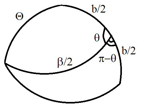
Figure 1: Geometrical meaning of the angle $\Theta$.

The $2\times 2$ matrix $B^{\prime}$ in terms of Euler angles reads

$$B^{\prime}=\left(\begin{array}[]{cc}(1+\cos^{2}\theta)\cos\beta\cos{b}-2\cos\theta\cos(a+\gamma)\sin\beta\sin{b}&-{\sqrt{3}}\,\sin^{2}\theta\cos{\beta}\\ -{\sqrt{3}}\,\sin^{2}\theta\cos{b}&-(1-3\cos^{2}{\theta})\end{array}\right)\,.$$ (92)

From (92) it follows that WF can be rewritten as a quadratic polynomial with respect to the variable $z=\cos\theta\,,$

$$W=\frac{4}{3}\left\{Az^{2}+Bz+C\right\}\,,$$ (93)

where

$$A = \frac{1}{2}\left[I_{3}\cos(\beta)+\sqrt{3}I_{8}\right]\left[\mu_{3}\cos(b)+\sqrt{3}\mu_{8}\right],$$ (94)

$$B = -I_{3}\mu_{3}\sin(\beta)\sin(b)\cos(a+\gamma),$$ (95)

$$C = \frac{1}{2}\,I_{3}\left[\mu_{3}\cos(b)-\sqrt{3}\mu_{8}\right]\cos(\beta)-\frac{\sqrt{3}}{2}\,I_{8}\left[\mu_{3}\cos(b)+\frac{1}{\sqrt{3}}\mu_{8}\right]+\frac{1}{4}\,.$$ (96)

$\bullet$ Reduction to $SU(2)$ symmetric SW spin-1 correspondence  $\bullet$ According to the Table 2 , the symmetry type of SW kernel and mixed state allowing to realize the sought reduction to $SU(2)/T^{1}$ is given by pairs of Young diagrams (1,1,1) and (2,1); the necessary value of sum of squares is $4\times 1\times 2=8$ describing SU(2) symmetric SW correspondence for spin-1 is:

$$(1,1,1)^{2}+(2,1)^{2}=3+5=8\,.$$

1. SW kernel with symmetry $S(U(2)\times U(1))\,.$ The expression for the Wigner function with ${S(U(2)\times U(1))}$ symmetric kernel follows from (92) when $\mu_{3}=0$ :

   $$W^{(2,1)}_{(1,1,1)}(\theta,\beta)=\frac{1}{3}+\frac{2}{3}\left[\sqrt{3}\,(I_{3}\cos\beta+\sqrt{3}\,I_{8})\cos^{2}{\theta}-(\sqrt{3}\,I_{3}\cos\beta+I_{8})\right]\,;$$ (97)

2. State with symmetry $S(U(2)\times U(1))\,.$ The expression for the Wigner function ${S(U(2)\times U(1))}$ symmetric state follows from (92) when $I_{3}=0$ :

   $$W^{(1,1,1)}_{(2,1)}(\theta,b)=\frac{1}{3}+\frac{2}{3}\,I_{8}\left[\sqrt{3}\,(\mu_{3}\cos\beta+\sqrt{3}\,\mu_{8})\cos^{2}{\theta}-(\sqrt{3}\,\mu_{3}\cos\beta+\mu_{8})\right]\,.$$ (98)

$\bullet$ Comments on the reduced phase-space $\bullet$ Note that the reduced WF in both cases, 1. and 2. , is definite on one fourth part of a unit sphere:

$$0\geq\theta\geq\frac{\pi}{2}\,,\quad 0\geq\beta\geq\pi\,.$$ (99)

According to the formulae (83)-(86) , the left action of the permutation matrix $P_{12}$ on the matrix $B$ can be dragged to the following shifts of angles $\theta$ and $\beta$:

$$P_{12}B(\theta,\beta,b)=B(\theta+\pi,\beta+\pi,b)\,,\qquad P_{12}=\begin{pmatrix}0&1&0\\ 1&0&0\\ 0&0&1\end{pmatrix}\,.$$ (100)

Therefore, the domain of definition of angles in (99) can be extended to cover a whole unit 2-sphere.

V Concluding remarks

In the present article we argue the existence of the unitary non-equivalent representations for the Stratonovich-Weyl kernels corresponding to the Wigner functions of arbitrary $N$- dimensional quantum system. The admissible Wigner functions can be classified by the values of $SU(n)$-invariant polynomials in the elements of the SW kernel. As it was shown, the “master equation” (16) fixes the values only of the lowest degree polynomial invariants, the first and second ones, while values of the remaining $N-2$ algebraically independent invariants distinguish members of the family of SW kernels.

In conclusion, it is necessary to mention that the present consideration of the quasiprobability functions makes no difference between elementary and composite systems. In forthcoming publications we will discuss in detail the Wigner functions for composite quantum systems, paying special attention to the manifestations of “quantumness”, particularly the entanglement BengtssonZyczkowskiBOOK , in properties of quasidistributions.

Apart from this, we leave for future studies interrelations between the reduction of WF described in the present note for a system possessing symmetries, with the corresponding Hamiltonian reduction on the phase-space of its classical counterpart.

*

Appendix A

A.1 The Gell-Mann basis of $\mathfrak{su}(3)$

The Gell-Mann basis $\{\lambda_{1},\lambda_{2},\dots,\lambda_{8}\}$ of the Lie algebra $\mathfrak{su}(3)$ reads:

$$\begin{array}[]{c}\begin{array}[]{ccc}\lambda_{1}=\left(\begin{array}[]{ccc}0&1&0\\ 1&0&0\\ 0&0&0\end{array}\right)\,,&\lambda_{2}=\left(\begin{array}[]{ccc}0&-i&0\\ i&0&0\\ 0&0&0\end{array}\right)\,,&\\ &&\\ \lambda_{3}=\left(\begin{array}[]{ccc}1&0&0\\ 0&-1&0\\ 0&0&0\end{array}\right)\,,&\lambda_{4}=\left(\begin{array}[]{ccc}0&0&1\\ 0&0&0\\ 1&0&0\end{array}\right)\,,&\\ &&\\ \lambda_{5}=\left(\begin{array}[]{ccc}0&0&-i\\ 0&0&0\\ i&0&0\end{array}\right)\,,&\lambda_{6}=\left(\begin{array}[]{ccc}0&0&0\\ 0&0&1\\ 0&1&0\end{array}\right)\,,\end{array}\\ \\ \begin{array}[]{cc}\lambda_{7}=\left(\begin{array}[]{ccc}0&0&0\\ 0&0&-i\\ 0&i&0\end{array}\right)\,,&\lambda_{8}=\displaystyle{\frac{1}{\sqrt{3}}}\left(\begin{array}[]{ccc}1&0&0\\ 0&1&0\\ 0&0&-2\end{array}\right)\,.\end{array}\end{array}$$ (101)

A.2 The adjoint action of the permutation matrix $T$

Consider the matrix which permutes the first and third diagonal elements of the $3\times 3$ identity matrix:

$$T=\left(\begin{array}[]{ccc}0&0&1\\ 0&1&0\\ 1&0&0\end{array}\right)\,.$$ (102)

The adjoint matrix $\mathrm{Ad}_{T}$ corresponding to the permutation (102), $T\lambda_{\mu}T=\left(\mathrm{Ad}_{{T}}\right)_{\mu\nu}\lambda_{\nu}\,,$ is

$$\mathrm{Ad}_{T}=\left(\begin{array}[]{cccc|cccc}0&0&0&0&0&1&0&0\\ 0&0&0&0&0&0&-1&0\\ 0&0&1/2&0&0&0&0&-\sqrt{3}/2\\ 0&0&0&1&0&0&0&0\\ \cline{1-8}\cr 0&0&0&0&-1&0&0&0\\ 1&0&0&0&0&0&0&0\\ 0&-1&0&0&0&0&0&0\\ 0&0&-\sqrt{3}/2&0&0&0&0&-1/2\end{array}\right)\,.$$ (103)

A.3 The adjoint vectors of SU(3)

Using the Euler decomposition (75), we determine the adjoint matrix $\mathrm{Ad}_{U}$ of SU(3) transformations $U$:

$$U\lambda_{i}U^{\dagger}=\left(\mathrm{Ad}_{U}\right)_{ij}\lambda_{j}\,,\qquad\mathrm{Ad}_{U}\in SO(8)\,.$$ (104)

Below, only expressions for vectors $n^{(3)}_{i}=(\mathrm{Ad}_{U})_{3i}$ and $n^{(8)}_{i}=(\mathrm{Ad}_{U})_{8i}$, specifying the Wigner function of a single qutrit (76), will be presented. Components of the vector $\bm{n}^{(8)}$ read:

$$\begin{array}[]{ccl}n^{(3)}_{1}&=&\Big{(}\sin(\alpha)\sin(a+\gamma)-\cos(\alpha)\cos(\beta)\cos(a+\gamma)\Big{)}\sin(b)\cos(\theta)+\cos(\alpha)\sin(\beta)\cos(b)\Big{(}1-\frac{1}{2}\sin^{2}(\theta)\Big{)},\\ &&\\ n^{(3)}_{2}&=&\Big{(}\cos(\alpha)\sin(a+\gamma)+\sin(\alpha)\cos(\beta)\cos(a+\gamma)\Big{)}\sin(b)\cos(\theta)+\sin(\alpha)\sin(\beta)\cos(b)\Big{(}1-\frac{1}{2}\sin^{2}(\theta)\Big{)},\\ &&\\ n^{(3)}_{3}&=&-\cos(a+\gamma)\sin(\beta)\sin(b)\cos(\theta)+\cos(\beta)\cos(b)\Big{(}1-\frac{1}{2}\sin^{2}(\theta)\Big{)},\\ &&\\ n^{(3)}_{4}&=&\cos\left(\frac{\alpha-\gamma}{2}-a\right)\sin\left(\frac{\beta}{2}\right)\sin(b)\sin(\theta)-\frac{1}{2}\cos\left(\frac{\alpha+\gamma}{2}\right)\cos\left(\frac{\beta}{2}\right)\cos(b)\sin(2\theta),\\ &&\\ n^{(3)}_{5}&=&\sin\left(\frac{\alpha-\gamma}{2}-a\right)\sin\left(\frac{\beta}{2}\right)\sin(b)\sin(\theta)+\frac{1}{2}\sin\left(\frac{\alpha+\gamma}{2}\right)\cos\left(\frac{\beta}{2}\right)\cos(b)\sin(2\theta),\\ &&\\ n^{(3)}_{6}&=&\cos\left(\frac{\alpha+\gamma}{2}+a\right)\cos\left(\frac{\beta}{2}\right)\sin(b)\sin(\theta)+\frac{1}{2}\cos\left(\frac{\alpha-\gamma}{2}\right)\sin\left(\frac{\beta}{2}\right)\cos(b)\sin(2\theta),\\ &&\\ n^{(3)}_{7}&=&\sin\left(\frac{\alpha+\gamma}{2}+a\right)\cos\left(\frac{\beta}{2}\right)\sin(b)\sin(\theta)+\frac{1}{2}\sin\left(\frac{\alpha-\gamma}{2}\right)\sin\left(\frac{\beta}{2}\right)\cos(b)\sin(2\theta),\\ &&\\ n^{(3)}_{8}&=&-\frac{\sqrt{3}}{2}\cos(b)\sin^{2}(\theta).\end{array}$$ (105)

The 8-vector $\bm{n}^{(8)}$ depends only on four angles $\{\alpha,\beta,\gamma,\theta\}$ and its components are:t4

$$\begin{array}[]{ccl}n^{(8)}_{1}&=&+\frac{\sqrt{3}}{2}\cos(\alpha)\sin(\beta)\sin^{2}(\theta),\\ &&\\ n^{(8)}_{2}&=&-\frac{\sqrt{3}}{2}\sin(\alpha)\sin(\beta)\sin^{2}(\theta),\\ &&\\ n^{(8)}_{3}&=&-\frac{\sqrt{3}}{2}\cos(\beta)\sin^{2}(\theta),\\ &&\\ n^{(8)}_{4}&=&-\frac{\sqrt{3}}{2}\cos\left(\frac{\alpha+\gamma}{2}\right)\cos\left(\frac{\beta}{2}\right)\sin(2\theta),\\ &&\\ n^{(8)}_{5}&=&+\frac{\sqrt{3}}{2}\sin\left(\frac{\alpha+\gamma}{2}\right)\cos\left(\frac{\beta}{2}\right)\sin(2\theta),\\ &&\\ n^{(8)}_{6}&=&+\frac{\sqrt{3}}{2}\cos\left(\frac{\alpha-\gamma}{2}\right)\sin\left(\frac{\beta}{2}\right)\sin(2\theta),\\ &&\\ n^{(8)}_{7}&=&+\frac{\sqrt{3}}{2}\sin\left(\frac{\alpha-\gamma}{2}\right)\sin\left(\frac{\beta}{2}\right)\sin(2\theta),\\ &&\\ n^{(8)}_{8}&=&1-\frac{3}{2}\sin^{2}(\theta).\end{array}$$ (106)

The 8-dimensional vector $\bm{n}^{\prime}$ in formula (IV.2) reads

$$\begin{array}[]{ccl}n_{1}^{\prime}&=&-\frac{\sqrt{3}}{2}\cos\left(\frac{\alpha^{\prime}-\gamma^{\prime}}{2}\right)\sin\left(\frac{\beta^{\prime}}{2}\right)\sin(2\theta^{\prime})\,,\\ &&\\ n_{2}^{\prime}&=&-\frac{\sqrt{3}}{2}\sin\left(\frac{\alpha^{\prime}-\gamma^{\prime}}{3}\right)\sin\left(\frac{\beta^{\prime}}{2}\right)\sin(2\theta^{\prime})\,,\\ &&\\ n_{3}^{\prime}&=&\frac{\sqrt{3}}{2}\left[\cos^{2}(\theta^{\prime})-\sin^{2}\left(\frac{\beta^{\prime}}{2}\right)\sin^{2}(\theta^{\prime})\right]\,,\\ &&\\ n_{4}^{\prime}&=&-\frac{\sqrt{3}}{2}\cos\left(\frac{\alpha^{\prime}+\gamma^{\prime}}{2}\right)\cos\left(\frac{\beta^{\prime}}{2}\right)\sin(2\theta^{\prime})\,,\\ &&\\ n_{5}^{\prime}&=&\frac{\sqrt{3}}{2}\sin\left(\frac{\alpha^{\prime}+\gamma^{\prime}}{2}\right)\cos\left(\frac{\beta^{\prime}}{2}\right)\sin(2\theta^{\prime})\,,\\ &&\\ n_{6}^{\prime}&=&\frac{\sqrt{3}}{2}\cos(\alpha^{\prime})\sin(\beta^{\prime})\sin^{2}(\theta^{\prime})\,,\\ &&\\ n_{7}^{\prime}&=&-\frac{\sqrt{3}}{2}\sin(\alpha^{\prime})\sin(\beta^{\prime})\sin^{2}(\theta^{\prime})\,,\\ &&\\ n_{8}^{\prime}&=&\frac{1}{2}\left[1-3\cos^{2}\left(\frac{\beta^{\prime}}{2}\right)\sin^{2}(\theta^{\prime})\right]\,.\end{array}$$ (107)

References

- (1) E. P. Wigner, On the quantum correction for thermodynamic equilibrium, Phys. Rev. 40, 749 (1932).
- (2) H. Weyl, Gruppentheorie und Quantenmechanik (Hirzel-Verlag, Leipzig, 1928).
- (3) H. J. Groenewold On the principles of elementary quantum mechanics, Physica 12, 405 (1946).
- (4) J. E. Moyal in Mathematical Proceedings of the Cambridge Philosophical Society, 1949, Quantum mechanics as a statistical theory 45 99.
- (5) M. Hillery, R. F. O’Connell, M. O. Scully and E. P. Wigner, Distribution functions in physics: Fundamentals, Phys. Rep., 106 121 (1984).
- (6) Klimov Andrei , and Hubert de Guise, General approach to quasi-distribution functions J. Phys. A. 43.40 402001 (2010).
- (7) Klimov, Andrei B., José Luis Romero, and Hubert de Guise, Generalized SU(2) covariant Wigner functions and some of their applications, J. Phys. A.50 323001.
- (8) D. J. Rowe, B. C. Sanders and H. de Guise, Representations of the Weyl group and Wigner functions for SU(3), J. Math. Phys. 40, 3604 (1999).
- (9) S. Chumakov, A. Klimov, and K. B. Wolf, Connection between two Wigner functions for spin systems Phys. Rev. A 61, 034101 (2000).
- (10) M. A. Alonso, G. S. Pogosyan, and K. B. Wolf, Wigner functions for curved spaces. I. On hyperboloids J. Math. Phys. 43, 5857 (2002).
- (11) A. I. Lvovsky and M. G. Raymer, Continuous-variable optical quantum-state tomography, Rev. Mod. Phys. 81, 299 (2009).
- (12) I. Rigas, L. L. Sánchez-Soto, A. B. Klimov, J. Rehacek and Z. Hradil, Orbital angular momentum in phase space Ann. Phys., 326 426 (2011).
- (13) T. Tilma, M. J. Everitt, J. H. Samson, W. J. Munro and K. Nemoto, Wigner functions for arbitrary quantum systems, Phys. Rev. Lett. 117, 180401 (2016).
- (14) R. L. Stratonovich, On distributions in representation space, Sov. Phys. JETP 4, 6, 891 (1957).
- (15) J. C. Varilly and J. M. Gracia-Bondia, The Moyal representation for spin, Ann. Phys. 190, 107(1989).
- (16) C. Brif and A. Mann, A general theory of phase-space quasiprobability distributions, J. Phys. A 31, L9 (1998).
- (17) C. Brif and A. Mann, Phase-space formulation of quantum mechanics and quantum-state reconstruction for physical systems with Lie-group symmetries, Phys. Rev. A 59 971(1999).
- (18) D. Weingarten, Asymptotic behavior of group integrals in the limit of infinite rank, J. Math. Phys. 19, 999 (1978).
- (19) B. Collins, Moments and cumulants of polynomial random variables on unitary groups, the Itzykson-Zuber integral, and free probability, Int. Math. Res. Not. 17, 953 (2003).
- (20) B. Collins and P. Sniady, Integration with respect to the Haar measure on unitary, orthogonal and symplectic group, Commun. Math. Phys. 264, 3, 773 (2006).
- (21) For example, in the quatrit case, any fixed order of eigenvalues corresponds to one out of 24 possible ways to tessellate a sphere by the spherical triangles whose angles are . Such a triangle is one of the four fundamental spherical Möbius Triangles with the tetrahedral symmetry, which is classified as a (2,3,3) triangle. Repeated reflections in the sides of the triangles will tile a sphere exactly once. In accordance with Girard’s theorem, the spherical excess of a triangle determines the solid angle:
- (22) Pedro de M. Rios and Eldar Straum, Symbol Correspondences for Spin Systems, Springer International Publishing, 2014.
- (23) I.Bengtsson, A.Ericsson, M.Kus, W.Tadej and K.Zyczkowski, Birkhoff’s polytope and unistochastic matrices, and . Communication Math. Phys. 259, 307–324 (2005)
- (24) A. Luis, SU(3) Wigner function for three-dimensional systems, J. Phys. A 41, 495302 (2008).
- (25) M. S. Byrd, Differential Geometry on SU(3) with applications to three state systems, J. Math. Phys. 39, 6125 (1998); M. S. Byrd, Erratum, J. Math. Phys. 41, 1026 (2000).
- (26) M. S. Byrd and E. C. G. Sudarshan, SU(3) Revisited, J. Phys. A 31, 9255 (1998).
- (27) V. Gerdt, R. Horan, A. Khvedelidze, M. Lavelle, D. McMullan and Palii Yu, On the Hamiltonian reduction of geodesic motion on SU(3) to SU(3)/SU(2), J. Math. Phys. 47, 112902 (2006).
- (28) I. Bengtsson and K. Zyczkowski, Geometry of Quantum States: An Introduction to Quantum Entanglement, (Cambridge University Press, 2006).