Quantum Annealing for Combinatorial Clustering

Abstract

Clustering is a powerful machine learning technique that groups “similar” data points based on their characteristics. Many clustering algorithms work by approximating the minimization of an objective function, namely the sum of within-the-cluster distances between points. The straightforward approach involves examining all the possible assignments of points to each of the clusters. This approach guarantees the solution will be a global minimum, however the number of possible assignments scales quickly with the number of data points and becomes computationally intractable even for very small datasets. In order to circumvent this issue, cost function minima are found using popular local-search based heuristic approaches such as $k$-means and hierarchical clustering. Due to their greedy nature, such techniques do not guarantee that a global minimum will be found and can lead to sub-optimal clustering assignments. Other classes of global-search based techniques, such as simulated annealing, tabu search, and genetic algorithms may offer better quality results but can be too time consuming to implement. In this work, we describe how quantum annealing can be used to carry out clustering. We map the clustering objective to a quadratic binary optimization (QUBO) problem and discuss two clustering algorithms which are then implemented on commercially-available quantum annealing hardware, as well as on a purely classical solver “qbsolv.” The first algorithm assigns $N$ data points to $K$ clusters, and the second one can be used to perform binary clustering in a hierarchical manner. We present our results in the form of benchmarks against well-known $k$-means clustering and discuss the advantages and disadvantages of the proposed techniques.

I Introduction

Clustering is the process of grouping objects based on their common features. It is a powerful machine learning technique used to digest and interpret data. Clustering algorithms find application in a wide variety of fields, including the investigation of gene expression patterns BenDor1999 ; Das2016 ; gorzalczany2016 ; marisa2013 , document clustering Xie2013 ; Balabantaray2015 , and consumer segmentation mudambi2002 ; sharma2013 ; chan2012 , among many others.

Often, clustering is cast as an optimization problem using an objective (or ‘cost’) function friedman2001elements . A common objective function is the sum over pairwise dissimilarities within the clusters:

$$W(C)=\frac{1}{2}\sum_{a=1}^{K}\sum_{C(i)=C_{a}}\sum_{C(i^{\prime})=C_{a}}d(x_{i},x_{i^{\prime}})$$ (1)

Here each $x_{i}$ represents an individual data point or observation, $d$ is a distance metric on the space of possible data points, and $C$ refers to the cluster assignment. Essentially, this results in a value given by the sum of the total distances between all points that reside in the same cluster. In combinatorial clustering, the total dissimilarity of every possible cluster assignment is examined to find the minimum of $W$, which guarantees a global minimum is found. Unfortunately, examining all possible assignments of observations to clusters is feasible only for very small datasets. For a task where $N$ data points are assigned to $K$ clusters, the number of distinct assignments is given by

$$S(N,K)=\frac{1}{K!}\sum_{i=1}^{K}(-1)^{K-i}{N\choose i}i^{N},$$ (2)

and for example, $S(19,4)\approx 10^{10}$ friedman2001elements . Even with modern computing resources, this exhaustive search technique quickly becomes impractical or outright impossible.

Common clustering algorithms, such as $k$-means hartigan1979 or hierarchical clustering johnson1967 are local search techniques which take less exhaustive, greedy approaches. For a nice summary of how clustering techniques have evolved, see jain2010 . Because they are heuristic-based greedy approaches, neither $k$-means nor hierarchical clustering are guaranteed to find an optimal clustering. A single run of the $k$-means algorithm is likely to end up with a locally optimal solution that is not a global optimum. Thus, $k$-means is typically run multiple times with different random initializations to get a subset of good solutions. The best solution is then chosen as the final clustering result. However, even with many runs, there is no guarantee that the true global minimum will be found, particularly if the solution space has many local minima.

The problem of choosing an optimal solution from many potential combinations, or combinatorial optimization, is well known in the computer science literature. Many formulations of the problem, including clustering, are NP-hard Garey1979 . These problems, including the famous traveling salesman problem, suffer from similar scaling issues papadimitriou1977 . For clustering related problems, global search techniques such as simulated annealing, tabu search, and genetic algorithms although computationally less efficient than $k$-means are known to produce better quality results al1996computational .

We discuss the simulated annealing (SA) kirkpatrick1983 based approach in a bit more detail, as it closely resembles the techniques we describe in this paper, and it has been widely used for clustering selim1991 . SA can be understood as analogous to the metallurgical process from which its name derives—slowly cooling a metal. During SA, the objective function is reimagined as the energy of a system. At all times, there are random transitions that can potentially occur. Which transitions actually occur is a function of both temperature and whether the transition would result in an increase or decrease in energy. At high temperatures, changes that increase or decrease the energy are almost equally likely, but as the temperature slowly decreases, energy increases become less and less likely, and eventually the system settles into a very low energy state.

In the context of clustering, SA starts with a random assignment of observations to different clusters. In each iteration, one observation is randomly chosen to be reassigned to a new cluster. The change in the objective function, or energy, $\Delta W=W_{\mathrm{new}}-W_{\mathrm{old}}$, caused by the reassignment is computed. If the energy decreases ($\Delta W<0$), the new assignment is accepted; if it increases ($\Delta W>0$), the new assignment is accepted with a probability proportional to $\mathrm{exp}(-\Delta W/T)$ where $T$ represents the “temperature” of the system. The process is continued for a predetermined number of steps, during which the temperature is reduced in some prescribed manner mitra1985 . At relatively high temperatures, the algorithm can easily increase its energy, escaping local minima. However, at low temperatures it steadily decreases in energy, eventually reaching a minimum. If the temperature is brought down slowly enough, the probability of arriving at the globally optimal clustering assignment approaches one.

SA-based clustering has shortcomings as well. It works well for moderate-sized data sets where the algorithm can traverse the energy landscape quickly. However, the process becomes extremely sluggish for large datasets, especially at low temperatures, and it becomes more likely to get stuck in local minima. In addition, there are several free parameters, and selecting a suitable cooling schedule is difficult and requires a time-consuming trial and error approach tuned to the problem at hand. There have been many attempts at improving the speed and quality of SA results szu1987 ; ingber1989 ; bouleimen2003 , generally by doing many sequential runs with a very short annealing schedule.

I.1 Quantum annealing

Quantum annealing (QA) is an outgrowth of simulated annealing that attempts to use quantum effects to improve performance kadowaki1998 . In QA, quantum fluctuations are used to change energy states, instead of SA’s thermal excitations. This has been thought to improve performance santoro2006 , and there have been some experimental results with recent commercially available devices to this effect denchev2016 .

In the adiabatic limit as the transformation from $H_{\mathrm{i}}$ to $H_{\mathrm{f}}$ slows sufficiently, the quantum annealer is guaranteed by the adiabatic theorem to finish in the ground state (if it begins in the ground state) Born1928 ; AlbashLidar2016 . In practice, real machines operate at finite temperature and it is impractical to set arbitrarily long annealing times. Moreover, the required annealing time is proportional to the spectral energy gap between the ground and first excited state, something that is rarely known a priori. Therefore it is common practice to perform multiple runs on the annealing device, each with a short (on the order of microseconds) annealing time, after which the solution and resulting energy is saved. After a large number of runs, the one with the lowest overall energy is selected as an approximation of the global minimum.

In order to use QA for optimization, one has to find a suitable mapping of the problem’s objective function to the energy states of a quantum system. Quantum annealing devices first initialize a quantum system in an easy-to-prepare ground state of an initial Hamiltonian $H_{\mathrm{i}}$, which is then slowly evolved into a final Hamiltonian $H_{\mathrm{f}}$ whose ground state corresponds to the solution of the optimization problem at hand; for example,

$$H(t)=(1-s(t))H_{\mathrm{i}}+s(t)H_{\mathrm{f}},\qquad 0\leq t\leq T$$ (3)

where $s$ is monotonically increasing with $s(0)=0$ and $s(T)=1$.

It has recently become possible to encode and solve real-life optimization problems on commercially available quantum annealing hardware biamonte2016quantum .Recent studies have demonstrated how QA can be used to carry out important machine learning tasks dulny2016developing ; neven2009nips ; denchev2013binary ; farinelli2016quantum including clustering kurihara2009quantum ; sato2013quantum . However, authors in Ref kurihara2009quantum ; sato2013quantum discuss a different class of "soft "clustering algorithms where a data point is probabilistically assigned to more than one cluster. Note that the algorithms presented in this work belong to the class of "hard" clustering algorithms where a data point is assigned to one and only one cluster.

Current generations of these devices are designed to solve problems cast into the form of an Ising spin glass Ising1925 :

$$H_{\text{f}}=\sum_{i}h_{i}\sigma_{i}+\sum_{ij}J_{ij}\sigma_{i}\sigma_{j}$$ (4)

Here $\sigma_{i}$ represents the state of the $i^{t\text{h}}$ qubit (or the $z$-component of the $i^{\text{th}}$ Pauli spin operator), and can take values $\pm 1$, while $h_{i}$ and $J_{ij}$ are the control parameters of the physical system and represent the bias on each of the qubits, and coupling between two qubits, respectively. A very similar problem, quadratic unconstrained binary optimization (QUBO), is also commonly used as a template. Ising problems can be trivially converted into QUBO and vice versa. In the next section we describe how the clustering objective function can be recast as a QUBO.

II Quantum Annealing Methods

II.1 One-hot encoding

Suppose $N$ points $\{x_{i}\}_{i=1}^{N}$ are to be assigned to $K$ clusters $\{C_{a}\}_{a=1}^{K}$. Let each point $x_{i}$ be associated with a Boolean variable $q_{a}^{i}$ which indicates whether the point is in cluster $C_{a}$ or not. We refer to this as a “one-hot” encoding, familiar from the QUBO solution of the map coloring problem Dahl2013 . Given the $\tfrac{1}{2}N(N-1)$ real, positive-valued separations $d(x_{i},x_{j})$, the clustering objective $W(C)$ can be written as

$$H^{\prime}=\tfrac{1}{2}{\textstyle\sum_{i,j=1}^{N}}d(x_{i},x_{j}){\textstyle\sum_{a=1}^{K}}q_{a}^{i}q_{a}^{j},$$ (5)

assuming one can guarantee that for each $i,$ only a single $q_{a}^{i}=1$ for some cluster label $a$, the rest being zero. Energetically-speaking however, with this form of $H^{\prime}$ the guarantee will not be honored, since the most beneficial values the $q$ may take are all zeroes (or at least such that $H^{\prime}$ remains zero). Thus we add constraints (one for each value of $i$) to the objective function in the form:

$$\phi^{i}=\left({\textstyle\sum_{a=1}^{K}}q_{a}^{i}-1\right)^{2}$$ (6)

times Lagrange multipliers $\lambda_{i}$ to $H^{\prime}$:

$$H :=H^{\prime}+{\textstyle\sum_{i=1}^{N}}\lambda_{i}\phi^{i}$$ (7)

$$={\textstyle\frac{1}{2}}{\textstyle\sum_{i,j=1}^{N}}d(x_{i},x_{j}){\textstyle\sum_{a=1}^{K}}q_{a}^{i}q_{a}^{j}+{\textstyle\sum_{i=1}^{N}}\lambda_{i}\left({\textstyle\sum_{a=1}^{K}}q_{a}^{i}-1\right)^{2},$$ (8)

In practice, we must ensure that the $\lambda_{i}$ are chosen large enough to discourage any constraint violation and force the one-hot encoding. In particular, we must protect against the mildest constraint violation, for which there are two possibilities: either a single $x_{i}$ can be assigned to more than one cluster, or it can be assigned to zero clusters.

If a point is assigned to more than one cluster, this can only result in an increase in $H$, simply because additional qubits being “switched on” can only introduce additional positive terms in the sum involving same-cluster distances $d(x_{i},x_{j})$. Therefore, this type of violation will never be favored energetically.

On the other hand, assigning $x_{i}$ to no cluster has the effect of setting some $d(x_{i},x_{j})$ to zero, thus reducing $H$. The goal then is to choose the corresponding $\lambda_{i}$ large enough so that the constraint term offsets the maximum possible reduction in $H$. When a point $x_{i}$ is assigned no cluster, in the worst-case scenario it can set $N-K$ pairwise-distances to zero (because $x_{i}$ could cluster with a maximum of $N-K$ points, assuming every cluster contains at least one point; we take as given that $N\geq K+1$). The maximum possible reduction in $H$ would result when each of the other points are at the maximum distance from $x_{i}$. In this case $H$ is reduced by

$$\sum_{x_{j}\in C_{a}}d(x_{i},x_{j})\leq(N-K)\cdot\max_{x_{j}\in C_{a}}(d(x_{i},x_{j}))$$ (9)

where the right-hand side is the worst-case scenario bound. Thus to guarantee that no constraint is violated, we set $\lambda_{i}=\lambda$ for all $i$ with

$$\lambda_{i}\geq(N-K)\tilde{d},$$ (10)

where $\tilde{d}$ is the pair-pointwise maximum of $d(x_{i},x_{j})$ for all $i,j$. In practice, one can normalize $d(x_{i},x_{j})$ so that $\tilde{d}=1$ in (10). Then setting $\lambda=(N-K)$ in (8) will ensure that no violations occur.

In practice, $\lambda$ cannot be made arbitrarily large. Ultimately this will make demands on one’s hardware precision, given the details of the clustering problem at hand. In the discussion that follows we comment on the precision limitations imposed by current-generation quantum annealing hardware specific to the one-hot encoding clustering approach.

If the hardware supports $n$-bit precision for the couplings and biases, and we assume only (dimensionless) integer values for those coefficients, then the coupling and bias values one might reliably set and distinguish are

$$\{-(2^{n-1}-1),-(2^{n-1}-2),\dots,-1,0,1,\dots,2^{n-1}-2,2^{n-1}-1\}.$$ (11)

To make a comparison with the hardware we will be using, we transform into spin variables.

II.1.1 Spin variables

To determine the couplings and biases one should use on the hardware annealer, or simulate this system, we must transform into spin variables $s_{a}^{i}=2q_{a}^{i}-1$, so set $q_{a}^{i}=\frac{1}{2}\left(s_{a}^{i}+1\right)$ in $H$ to obtain (we drop constants along the way)

$$H = \tfrac{1}{2}{\textstyle\sum_{a=1}^{K}\sum}{}_{i,j=1}^{N}d(x_{i},x_{j})\tfrac{1}{2}(s_{ia}+1)\tfrac{1}{2}(s+1)$$

$$= \tfrac{1}{8}{\textstyle\sum}_{a=1}^{K}{\textstyle\sum}_{i,j=1}^{N}d(x_{i},x_{j})s_{a}^{i}s_{a}^{j}+\tfrac{1}{4}\lambda{\textstyle\sum_{i=1}^{N}}{\textstyle\sum_{a\neq b}}s_{a}^{i}s_{b}^{i}$$

$$+\tfrac{1}{4}{\textstyle\sum}_{i,j=1}^{N}d(x_{i},x_{j}){\textstyle\sum}_{a=1}^{K}s_{a}^{i}+\tfrac{1}{2}\lambda(K-2){\textstyle\sum}_{i=1}^{N}{\textstyle\sum}_{a=1}^{K}s_{a}^{i},$$

where we have used $\sum_{a\neq b}\left(s_{a}^{i}+s_{b}^{i}\right)=2(K-1)\sum_{a}s_{a}^{i}.$ The double sums are only over unique pairs, so we may write (introducing an overall scaling)

$$H = \tfrac{1}{2}{\textstyle\sum}_{a=1}^{K}{\textstyle\sum}_{(i,j)}d(x_{i},x_{j})s_{a}^{i}s_{a}^{j}+\lambda{\textstyle\sum}_{i=1}^{N}{\textstyle\sum}_{(a,b)}s_{a}^{i}s_{b}^{i}$$

$$+{\textstyle\sum}_{(i,j)}d(x_{i},x_{j}){\textstyle\sum}_{a=1}^{K}s_{a}^{i}+2\lambda(K-2){\textstyle\sum}_{i=1}^{N}{\textstyle\sum}_{a=1}^{K}s_{a}^{i}.$$

We want to maximize $\lambda$ given the hardware constraints. When $K>2$ and the hardware is precise to $n$-bits, we thus set

$$2\lambda(K-2)=2^{n-1}-1$$

or

$$\lambda=\frac{2^{n-1}-1}{2(K-2)}.$$ (12)

and $H$ becomes

$$H = \tfrac{1}{8}{\textstyle\sum}_{a=1}^{K}{\textstyle\sum}_{i,j=1}^{N}d(x_{i},x_{j})s_{ia}s_{ja}+\frac{2^{n-1}-1}{K-2}{\textstyle\sum}_{i=1}^{N}{\textstyle\sum}_{b>a=1}^{K}s_{ia}s_{ib}$$

$$+\tfrac{1}{8}{\textstyle\sum}_{i,j=1}^{N}d(x_{i},x_{j}){\textstyle\sum}_{a=1}^{K}\left(s_{ia}+s_{ja}\right)+\left(2^{n-1}-1\right){\textstyle\sum}_{i=1}^{N}{\textstyle\sum}_{a=1}^{K}s_{ia}.$$

The scaling requirement for $d$ reads

$$\left|d\right|\leq\frac{2\left(2^{n-1}-1\right)}{(N-K)\left(K-2\right)}.$$

For $n=6$ (which is the precision on current commercially available quantum annealers), this is

$$\left|d\right|\leq\frac{62}{(N-K)\left(K-2\right)}.$$

For the minuscule test case $N=4$ and $K=3,$ one just needs to have the maximum $d\leq 62,$ but the couplings involving $d$ appear as $\frac{1}{8}d,$ so these are restricted to be $<8,$ which doesn’t leave much room for accuracy. Clearly things only get worse as $N$ grows. For this reason, current QA hardware with six bits of precision may only reliably accommodate small clustering instances. In the next section we describe another QUBO formulation of the clustering objective which enables us to carry out binary clustering and removes the precision limitations posed by the one-hot encoding technique.

II.2 Binary Clustering

In order to develop a better intuition we use spin variables here. Suppose $N$ points are to be assigned to $K=2$ clusters. Let each point $x_{i}$ be associated with an Ising variable $s_{i}=\pm 1$ which indicates whether the point is in cluster 1 ($s_{i}=1$) or not ($s_{i}=-1$). We refer to this as binary clustering. Without the one-hot constraint, the objective is simply

$$H=\frac{1}{2}\sum_{i,j=1}^{N}d(x_{i},x_{j})s_{i}s_{j}.$$

When $d(x_{i},x_{j})$ is large, $s_{i}$ and $s_{j}$ tend to adopt opposite spins (and thus are assigned to different clusters), whereas if $d(x_{i},x_{j})$ is small, points tend to adopt the same spin (and thus are assigned to the same cluster). This approach allows assignment of points to only $K=2$ clusters as opposed the one-hot encoding case. However, since there are no constraints, the precision issues faced by one-hot encoding are avoided. Moreover, it requires a significantly smaller number of qubits (half if we compare with $K=2$ one-hot encoding). To accommodate more clusters, one can envision running this approach recursively along with a divisive hierarchical clustering scheme.

One might ask why we don’t use a binary encoding of cluster membership for $K>2.$ Indeed, this would be a thrifty use of qubits. Unfortunately, in this case the objective function exceeds quadratic order in the $s_{i}$, so it is not immediately amenable to solution on D-Wave 2X hardware. There exist methods for reducing the order reduction , but at the expense of introducing additional qubits, the number of which scales worse than the number in the one-hot encoding. The question of whether the relaxed precision demands encountered using this order reduction method gives some edge is left for future investigation.

III Results

III.1 One-hot encoding

Here we present our clustering results obtained using one-hot encoding as well as binary clustering technique. For problem sizes that fit onto the hardware, results were obtained by running on actual QA hardware. For larger instances which cannot fit, an open-source solver qbsolv was used. Qbsolv was recently released by D-Wave Booth2009 and allows QUBO problems that are too large to be embedded onto QA devices to be solved. It is a hybrid approach that is designed to be able to use the best of both classical and quantum optimization. First, in the classical step, the large QUBO is divided into smaller sub-QUBOs. Then each of these smaller sub-QUBOs can be solved by QA. These solutions are then stitched back together to find a full solution. In this paper qbsolv is used as a purely classical technique using tabu search as a solver instead of QA.

We use $k$-means clustering to compare performance. We first start with a customized pedagogical problem to develop intuition of how $k$-means can fail while the quantum-based approach succeeds. This particular problem highlights the issue of improper initialization of centroids during $k$-means which leads sub-optimal solutions. Figure (1) a), b) and c) show the clustering of 12 points among four clusters using $k$-means.

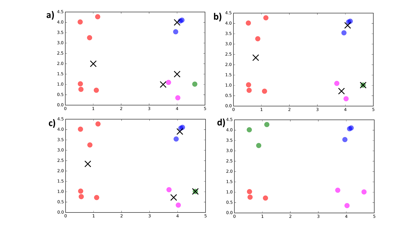
Figure 1: Clustering assignments obtained by $k$-means and one-hot encoding. The color coding represents clustering assignment. The black crosses indicate centroid position. a), b), c) indicate assignments obtained using $k$-means at iteration number 1, 2, and 20, respectively. d) indicates the assignment obtained using one-hot encoding run on the QA hardware.

We show here a specific initialization of centroids. In this particular configuration, where one centroid is centered in between a pair of clusters, while the other three centroids are shared near the other two true clusters. As can be seen, this can cause $k$-means to fail, converging to the local minimum seen in Figure (1 c). Note that such unfortunate initializations occur more frequently when data points belong to $p>2$ dimensional space. Thus while this particular instance is trivially solved by repeating with multiple random initializations, in higher dimensions the problem becomes more common and severe. Figure 1d) indicates clustering obtained using the one-hot encoding running on QA hardware.

One-hot encoding is able to cluster points in a single step compared to the iterative procedure followed by $k$-means. This instance required 48 variables encoded on the hardware which are partially connected to each other. The appropriate embedding was found by the heuristic embedding solver provided on the QA hardware. For all cases, QA hardware was run with default parameters and post-processing was switched off. Unless stated otherwise, in all cases 1000 samples were collected and the spin configuration with lowest energy was selected as the optimal solution. The couplings and biases were initially input in QUBO form. For all instances, $d(x_{i},x_{j})$ was scaled to lie within the range $[0,1]$. For all one-hot encoding instances, $\lambda$ was set equal to $N$ to satisfy the constraint 12.

We also used the one-hot encoding technique with qbsolv to solve larger instances. We carried out clustering of $N=200,1000,$ and 2000 points into $K=6$ clusters using one-hot and $k$-means. The points were created as Gaussian blobs where overlap between clusters was allowed. The scikit-learn scikit-learn implementation of $k$-means was used for comparison purposes. During $k$-means, the centroid initialization was done randomly as well as using the $k$-means++ technique arthur2007k . Ten initializations were used and the one with lowest “inertia” was considered as the solution. Inertia refers to the sum of distances between points and their respective cluster centroid and is different from $W$. In $W$, each such distance is weighted by the cluster size as well. $k$-means was considered to have converged when the difference in inertia between successive iterations reached $10^{-4}$ or 300 iterations were completed. Figure (2) indicates the clustering assignments obtained using one-hot encoding and $k$-means for $N=200$ and $2000$ case.

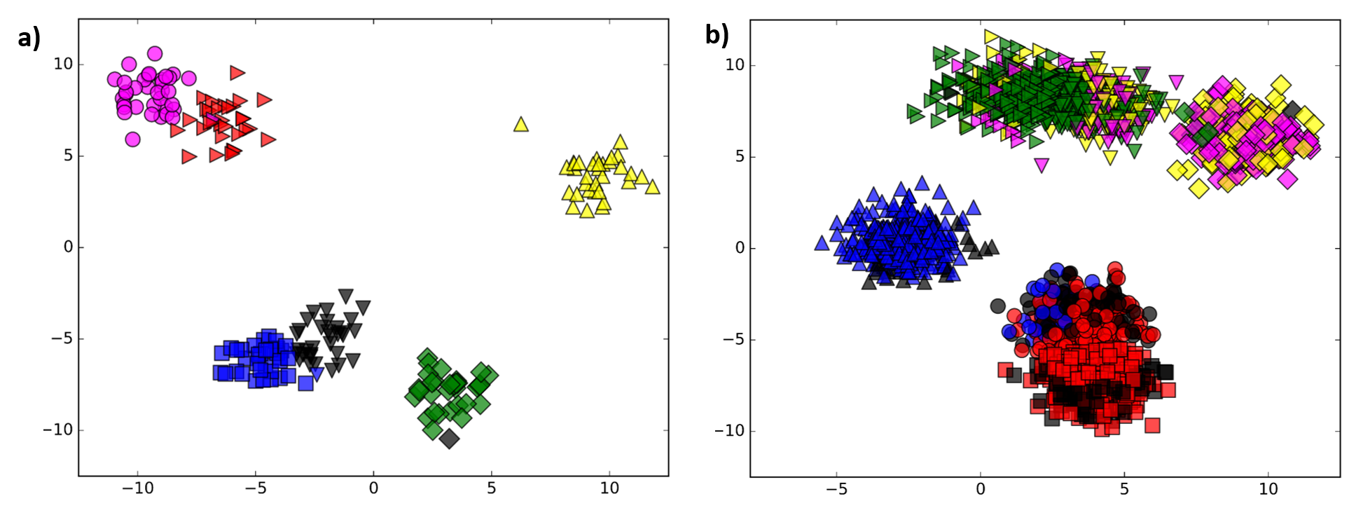
Figure 2: Clustering assignments obtained using $k$-means and one-hot encoding. The color coding represents cluster assignment obtained by one-hot encoding whereas marker shape represents cluster assignment obtained using $k$-means. a) and b) indicate $N=$ 200 and 2000 case. One-hot encoding was run using qbsolv with nrepeat $=50$.

For $N=200$ case, one-hot encoding achieves assignments similar to $k$-means. Whereas, the $N=2000$ case indicates major differences between the assignments obtained using both the techniques. In order to quantify these differences, in Table 1 we compare the inertia values obtained using one-hot encoding and $k$-means.

Table 1: Inertia values obtained using $k$-means and one-hot encoding

N	$k$-means++	random	one-hot encoding
200	342.88	342.88	402.78
1000	1923.81	1923.84	4336.72
2000	3622.99	3622.99	15164.98

The first two columns in Table 1 refer to the two different ways in which centroids were initialized during $k$-means. It is clear that in all cases, $k$-means outperforms one-hot encoding. The performance of $k$-means is much better than the one-hot encoding for $N=1000$ and $2000$ cases. This trend was somewhat expected as $N=1000$ and $2000$ cases involve optimization of systems containing $6000$ and $12000$ variables respectively. The quality of clustering obtained using one-hot encoding depends heavily on the quality of solution obtained using a given solver. We believe that the system sizes studied here are simply too large for qbsolv to handle.

We used qbsolv as a blackbox in order to assess the performance of proposed algorithms. In order to further examine the influence of qbsolv’s solution quality on clustering, we ran qbsolv with different values of the parameter nrepeat. nrepeat is a hyperparameter in the qbsolv solver. It is expected that setting nrepeat to a higher value than the default value would return better quality solutions. Figure (3) indicates the evolution of inertia with the parameter nrepeat for $N=200$ case.

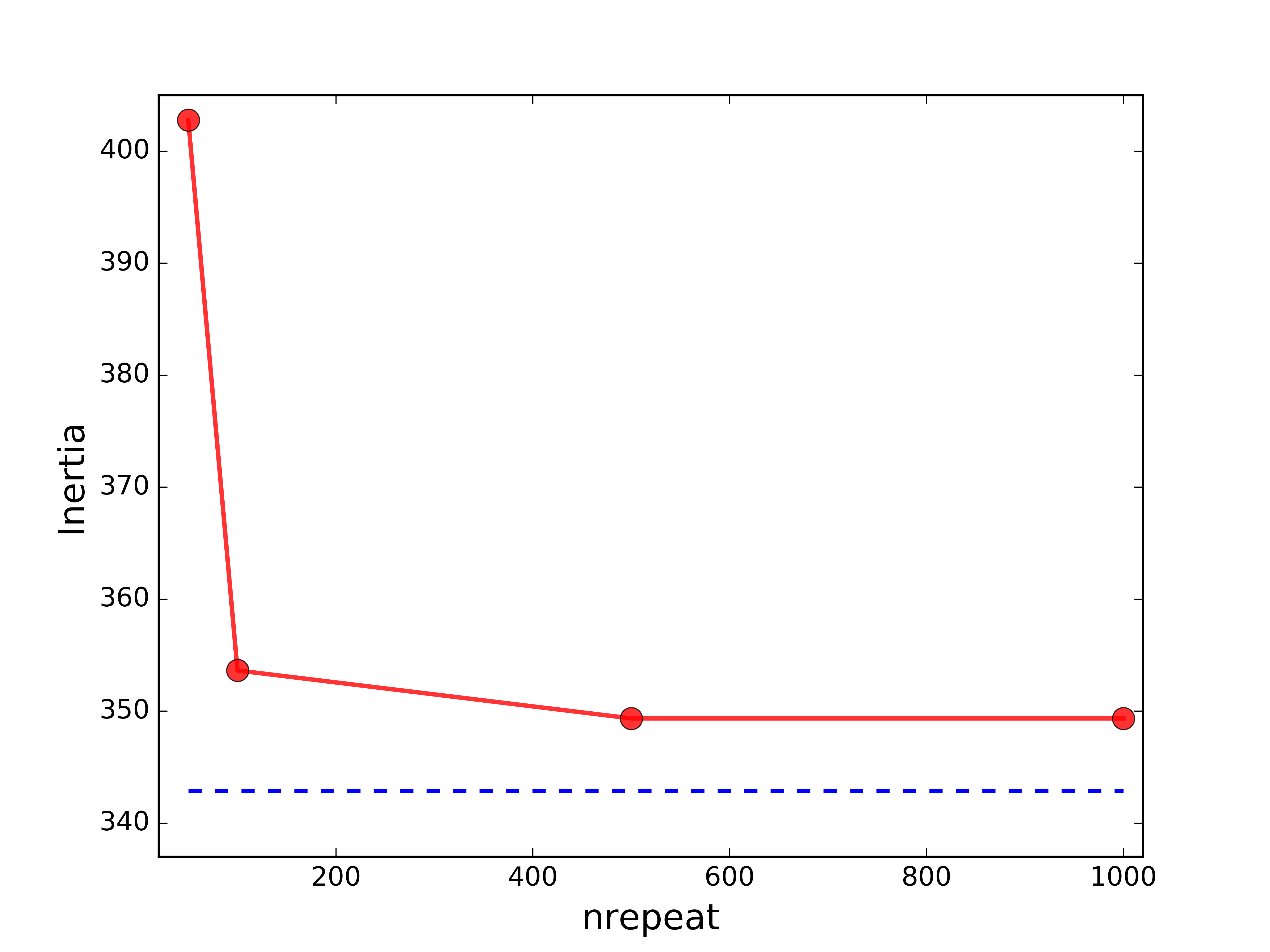
Figure 3: Evolution of inertia with nrepeat parameter. Red circles represent inertia values obtained using one-hot encoding and qbsolv. The red line serves as a guide to the eye. The dashed blue line indicates inertia value obtained using $k$-means.

The clustering performance improves and gets closer to the $k$-means performance as nrepeat value is increased. We obtained diminishing improvements as nrepeat value was further increased. This clearly indicates that as the solver gets better, the performance of the one-hot encoding algorithm improves. We believe there are other qbsolv hyperparameters which can be fine-tuned to achieve better results. A detailed study is needed to understand the influence of hyperparameters on the quality of solutions obtained using qbsolv.

III.2 Binary Clustering

We present our results for the binary clustering case. For binary clustering we generate data points uniformly over an ellipse. Such a distribution of points in two dimensions is known to be equivalent to clustering of Gaussian distributed points in higher dimensions, a fact that was used in savaresi2001performance to compare the performance of bisecting $k$-means and principal direction divisive partitioning (PDDP). Figure (4) indicates a comparison between $k$-means and binary clustering method for $N=40$ and $2000$.

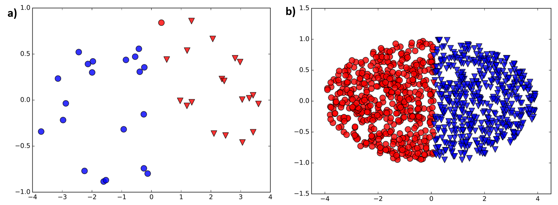
Figure 4: Clustering assignments obtained using $k$-means and binary clustering. The color coding represents the cluster assignment obtained by binary clustering whereas the marker shape represents the cluster assignment obtained using $k$-means. a) and b) show $N=200$ and 2000.

The binary clustering for $N=40$ was run on QA hardware. 40 fully connected variables were embedded on the hardware using D-Wave’s heuristic embedding solver cai2014practical . The $N=1000$ and $2000$ cases were treated using qbsolv. We observe few differences in the cluster labels obtained using $k$-means and binary clustering. This is evident from the inertia values obtained for both the techniques tabulated in Table 2.

Table 2: Inertia values obtained using $k$-means and binary clustering.

N	$k$-means++	random	binary clustering
40	52.81	52.81	52.89
1000	1330.90	1330.90	1330.94
2000	2784.07	2784.08	2784.14

Inertia values obtained using binary clustering are very close to those obtained using $k$-means. The performance of binary clustering does not appear to get as low as the data size increases compared to one-hot encoding.

IV Discussion

In this paper we introduced two formulations of the clustering objective function which can be used to carry out clustering on quantum annealing hardware. The one-hot encoding technique’s performance was poor compared to the $k$-means clustering on relatively large datasets. Our study indicates that one-hot encoding yields better results as solver quality improves. The need to use constraints severely limits the use of one-hot encoding on QA hardware for clustering of all but very small datasets due to the precision requirement. Moreover, one-hot encoding requires substantially more qubits to encode the problem. The one-hot encoding scheme adopted here, where each data point is associated to a $K$-bit string, does not use the qubits efficiently and leads to cumbersome constraint conditions. One could imagine a more efficient use of qubits to avoid or decrease the dependency on constraints by using a binary encoding-based scheme. In a binary encoding formulation, cluster assignment for each data point can be represented by binary strings. Further investigation in this direction is ongoing.

We tried to relax the constraint condition by setting $\lambda<(N-k)$. As the constraint was relaxed we started observing violations where a given point was assigned to more than one cluster. These solutions were considered invalid in the current implementation. However there are classes of fuzzy clustering algorithms where data points are allowed to be assigned to more than one cluster. How such fuzzy frameworks can be aligned with the current technique is not clear and requires further investigation.

The binary clustering was observed to compare well with the $k$-means results. The absence of constraints and use of fewer qubits makes it particularly suitable for clustering of large datasets. These advantages come with a limitation that binary clustering can only be used to carry out binary splits at each step. We expect that in algorithms such as divisive hierarchical clustering which makes binary split at each step, one can benefit from the binary clustering technique. Binary splitting in itself is an NP-hard problem and has traditionally been treated with heuristic algorithms during divisive hierarchical clustering Guenoche1991 . Hence, a hierarchical clustering approach, in conjunction with binary clustering is expected to outperform the current versions of divisive hierarchical clustering algorithms. Any such comparison of the techniques introduced here with hierarchical clustering and other advanced algorithms such as PDDP is left to a future study.

- [1] Amir Ben-Dor, Ron Shamir, and Zohar Yakhini. Clustering gene expression patterns. Journal of computational biology, 6(3-4):281–297, 1999.
- [2] Ranjita Das and Sriparna Saha. Gene expression data classification using automatic differential evolution based algorithm. In Evolutionary Computation (CEC), 2016 IEEE Congress on, pages 3124–3130. IEEE, 2016.
- [3] Marian B Gorzałczany, Filip Rudzínski, and Jakub Piekoszewski. Gene expression data clustering using tree-like soms with evolving splitting-merging structures. In Neural Networks (IJCNN), 2016 International Joint Conference on, pages 3666–3673. IEEE, 2016.
- [4] Laetitia Marisa, Aurélien de Reyniès, Alex Duval, Janick Selves, Marie Pierre Gaub, Laure Vescovo, Marie-Christine Etienne-Grimaldi, Renaud Schiappa, Dominique Guenot, Mira Ayadi, et al. Gene expression classification of colon cancer into molecular subtypes: characterization, validation, and prognostic value. PLoS Med, 10(5):e1001453, 2013.
- [5] Pengtao Xie and Eric P. Xing. Integrating document clustering and topic modeling. CoRR, abs/1309.6874, 2013.
- [6] Rakesh Chandra Balabantaray, Chandrali Sarma, and Monica Jha. Document clustering using k-means and k-medoids. CoRR, abs/1502.07938, 2015.
- [7] Susan Mudambi. Branding importance in business-to-business markets: Three buyer clusters. Industrial marketing management, 31(6):525–533, 2002.
- [8] Arun Sharma and Douglas M Lambert. Segmentation of markets based on customer service. International Journal of Physical Distribution & Logistics Management, 2013.
- [9] Kit Yan Chan, CK Kwong, and Bao Qing Hu. Market segmentation and ideal point identification for new product design using fuzzy data compression and fuzzy clustering methods. Applied Soft Computing, 12(4):1371–1378, 2012.
- [10] Jerome Friedman, Trevor Hastie, and Robert Tibshirani. The elements of statistical learning, volume 1. Springer series in statistics New York, 2001.
- [11] John A Hartigan and Manchek A Wong. Algorithm as 136: A k-means clustering algorithm. Journal of the Royal Statistical Society. Series C (Applied Statistics), 28(1):100–108, 1979.
- [12] Stephen C Johnson. Hierarchical clustering schemes. Psychometrika, 32(3):241–254, 1967.
- [13] Anil K Jain. Data clustering: 50 years beyond k-means. Pattern recognition letters, 31(8):651–666, 2010.
- [14] Michael R. Garey and David S. Johnson. Computers and Intractability: A Guide to the Theory of NP-Completeness. W. H. Freeman & Co., New York, NY, USA, 1979.
- [15] Christos H Papadimitriou. The euclidean travelling salesman problem is np-complete. Theoretical computer science, 4(3):237–244, 1977.
- [16] Khaled S Al-Sultana and M Maroof Khan. Computational experience on four algorithms for the hard clustering problem. Pattern recognition letters, 17(3):295–308, 1996.
- [17] Scott Kirkpatrick, C Daniel Gelatt, Mario P Vecchi, et al. Optimization by simulated annealing. science, 220(4598):671–680, 1983.
- [18] Shokri Z Selim and K1 Alsultan. A simulated annealing algorithm for the clustering problem. Pattern recognition, 24(10):1003–1008, 1991.
- [19] Debasis Mitra, Fabio Romeo, and Alberto Sangiovanni-Vincentelli. Convergence and finite-time behavior of simulated annealing. In Decision and Control, 1985 24th IEEE Conference on, volume 24, pages 761–767. IEEE, 1985.
- [20] Harold Szu and Ralph Hartley. Fast simulated annealing. Physics letters A, 122(3-4):157–162, 1987.
- [21] Lester Ingber. Very fast simulated re-annealing. Mathematical and computer modelling, 12(8):967–973, 1989.
- [22] KLEIN Bouleimen and HOUSNI Lecocq. A new efficient simulated annealing algorithm for the resource-constrained project scheduling problem and its multiple mode version. European Journal of Operational Research, 149(2):268–281, 2003.
- [23] Tadashi Kadowaki and Hidetoshi Nishimori. Quantum annealing in the transverse ising model. Physical Review E, 58(5):5355, 1998.
- [24] Giuseppe E Santoro and Erio Tosatti. Optimization using quantum mechanics: quantum annealing through adiabatic evolution. Journal of Physics A: Mathematical and General, 39(36):R393, 2006.
- [25] Vasil S Denchev, Sergio Boixo, Sergei V Isakov, Nan Ding, Ryan Babbush, Vadim Smelyanskiy, John Martinis, and Hartmut Neven. What is the computational value of finite-range tunneling? Physical Review X, 6(3):031015, 2016.
- [26] M. Born and V. Fock. Beweis des Adiabatensatzes. Zeitschrift fur Physik, 51:165–180, March 1928.
- [27] T. Albash and D. A. Lidar. Adiabatic Quantum Computing. ArXiv e-prints, November 2016.
- [28] J. Biamonte, P. Wittek, N. Pancotti, P. Rebentrost, N. Wiebe, and S. Lloyd. Quantum Machine Learning. ArXiv e-prints, November 2016.
- [29] J. Dulny, III and M. Kim. Developing Quantum Annealer Driven Data Discovery. ArXiv e-prints, March 2016.
- [30] Harmut Neven, Vasil S Denchev, Marshall Drew-Brook, Jiayong Zhang, William G Macready, and Geordie Rose. Nips 2009 demonstration: Binary classification using hardware implementation of quantum annealing. Quantum, pages 1–17, 2009.
- [31] Vasil S Denchev. Binary classification with adiabatic quantum optimization. PhD thesis, Purdue University, 2013.
- [32] Alessandro Farinelli. A quantum annealing approach to biclustering. In Theory and Practice of Natural Computing: 5th International Conference, TPNC 2016, Sendai, Japan, December 12-13, 2016, Proceedings, volume 10071, page 175. Springer, 2016.
- [33] Kenichi Kurihara, Shu Tanaka, and Seiji Miyashita. Quantum annealing for clustering. In Proceedings of the Twenty-Fifth Conference on Uncertainty in Artificial Intelligence, pages 321–328. AUAI Press, 2009.
- [34] Issei Sato, Shu Tanaka, Kenichi Kurihara, Seiji Miyashita, and Hiroshi Nakagawa. Quantum annealing for dirichlet process mixture models with applications to network clustering. Neurocomputing, 121:523–531, 2013.
- [35] Ernst Ising. Beitrag zur theorie des ferromagnetismus. Zeitschrift für Physik, 31(1):253–258, Feb 1925.
- [36] ED Dahl. Programming with d-wave: Map coloring problem (2013), 2013.
- [37] H. Ishikawa. Transformation of general binary mrf minimization to the first-order case. IEEE Transactions on Pattern Analysis and Machine Intelligence, 33(6):1234–1249, June 2011.
- [38] Michael Booth, Steven P. Reinhardt, and Aidan year="2009" Roy. Partitioning optimization problems for hybrid classical/quantum execution.
- [39] F. Pedregosa, G. Varoquaux, A. Gramfort, V. Michel, B. Thirion, O. Grisel, M. Blondel, P. Prettenhofer, R. Weiss, V. Dubourg, J. Vanderplas, A. Passos, D. Cournapeau, M. Brucher, M. Perrot, and E. Duchesnay. Scikit-learn: Machine learning in Python. Journal of Machine Learning Research, 12:2825–2830, 2011.
- [40] David Arthur and Sergei Vassilvitskii. k-means++: The advantages of careful seeding. In Proceedings of the eighteenth annual ACM-SIAM symposium on Discrete algorithms, pages 1027–1035. Society for Industrial and Applied Mathematics, 2007.
- [41] Sergio M Savaresi and Daniel L Boley. On the performance of bisecting k-means and pddp. In Proceedings of the 2001 SIAM International Conference on Data Mining, pages 1–14. SIAM, 2001.
- [42] Jun Cai, William G Macready, and Aidan Roy. A practical heuristic for finding graph minors. arXiv preprint arXiv:1406.2741, 2014.
- [43] A. Guénoche, P. Hansen, and B. Jaumard. Efficient algorithms for divisive hierarchical clustering with the diameter criterion. Journal of Classification, 8(1):5–30, Jan 1991.