Auxiliary Space Multigrid Method Based on Additive Schur Complement Approximation for Graph Laplacian

Abstract.

This research studies the application of the auxiliary space multigrid method (ASMG) that is based on additive Schur complement approximation (ASCA) to graph Laplacian matrices arising from general graphs. A major predicament when considering algebraic multigrid (AMG) methods on such graphs is the choice of a general coarsening strategy which has to be both cheap and effective. Such a strategy has been incorporated in the presented approach which in addition has several advantages. First, it is purely algebraic in its construction which makes the algorithm easy to implement. Furthermore, the approach requires no limitation on the graph’s structure and itself can be adjusted to the particular problem. Last but not least, its computational complexity can be easily analysed. A demonstrative set of numerical experiments is presented.

1. Introduction

Laplacian matrices of graphs have a wide range of applications including, but not limited to, machine learning, clustering in images, data mining, see e.g. [1, 2, 3, 4, 5]. Additionally, they also play an important role in finite element and finite difference discretizations of elliptic partial differential equations (PDEs) describing various physical phenomena. A structured and detailed overview about their significance could be found, for example, in the work of Spielman [6].

As would be expected, the design and development of fast solvers for corresponding linear systems has been the focus of considerable research where multilevel/multigrid algorithms have been of particular interest. Notable results include aggregation-based, see e.g. [7, 8, 9, 10], and disaggregation-based AMG preconditioners, see e.g. [11], accelerated, [12], and combinatorial multigrid and multilevel preconditioners, see [13, 14]. In [7] Livne and Brandt have introduced the lean algebraic multigrid method based on aggregation motivated by a new vertex proximity measure and simple piecewise constant prolongators coupled with an energy correction procedure applied to coarse-level systems. Brannick et al. have presented estimates of the convergence rate and complexity of an AMG preconditioner based on piecewise constant coarse vector spaces applied to the graph Laplacian, see [8]. The approach proposed in [9] combines aggressive coarsening based on aggregation with a polynomial smoother with sufficiently large degree to solve Laplacian systems arising from the standard linear finite element discretization of the scalar Poisson problem. More recently, Napov and Notay, see [10], have developed an aggregation based multigrid method that relies on the recursive static elimination of the vertices of degree $1$ combined with a new Degree-aware Rooted Aggregation (DRA) algorithm. The adaptive algebraic multigrid method proposed by D’Ambra and Vassilevski for solving Graph Laplacians, see [11], relies on a disaggregation technique where the few high degree nodes are broken into multiple smaller degree nodes. The authors of [12] offer multigrid type techniques that combine ad hoc coarser-grid operators with iterative techniques used as smoothers for the numerical solution of graph Laplacian operators. The results presented in [13, 14] suggest an approach to construct multigrid-like solvers based on support theory principles. Graph Laplacian preconditioners have been studied in [6] and [15] where graph sparsification techniques have been used to maintain reasonable computational complexity in the case of general large graphs.

The solver advocated here results from the interplay between graph and multigrid theory which makes it universal from the view point of applicability and construction. The utilized multigrid method is based on the additive Schur complement approximation (ASCA), see [16], used to construct coarse spaces and auxiliary-space correction, see [17, 18, 19], which replaces the standard multigrid coarse-grid correction. Finding maximal independent subsets (MIS) in graphs is essential for the proposed auxiliary space multigrid algorithm as they specify not only the coarse-fine splitting of the degrees of freedom, as e.g. in [20, 21], but also the construction of ASCA.

The rest of the paper is organized as follows. In Section 2 the graph Laplacian model problem is presented, the basic notations are introduced and a procedure generating the building components of the multigrid method is described. The next section, Section 3, includes the definitions of the ASCA and the auxiliary space multigrid algorithm. The complexity of the proposed algorithm has been discussed in Section 4. A demonstrative set of experiments is presented in Section 5. Finally, some concluding remarks have been made.

2. Problem formulation

2.1. Description and assumptions

Consider the undirected graph $K$ comprising the set of vertices, also known as nodes, $\mathcal{V}$ together with the set of edges $\mathcal{E}$ (which are $2$-element subsets of $\mathcal{V}$)

$$K=(\mathcal{V},\mathcal{E}),$$

where $|\mathcal{V}|=n$ and $|\mathcal{E}|=m$. In what follows, we further assume that $K$ is an unweighted and connected graph. Our aim is to solve the linear system

(1) $$A{\text{{u}}}={\text{{f}}}$$

where ${\text{{f}}}\in\text{Range}(A)$ while $A$ is the Laplacian matrix related to the graph $K$ as

$$(A)_{ij}=\begin{cases}\;\,d_{i}\qquad\qquad i=j;\\[2.2pt] -1\qquad\qquad i\neq j,\,(i,j)\in\mathcal{E};\\[2.2pt] \;\;\;0\qquad\qquad i\neq j,\,(i,j)\notin\mathcal{E}.\end{cases}$$

Here $d_{i}$ denotes the degree of the $i$-th vertex.

Obviously, $A$ is a symmetric, positive semi-definite (SPSD), singular M-matrix whose kernel is spanned by the constant vector 1. One way to deal with the semi-definiteness of the problem is to apply a rank-$1$ update of the matrix, thereby obtaining an equivalent SPD problem, see [11] for more details. Another remedy is the application of a deflated version of the conjugate gradient (CG) method to maintain the residuals orthogonal to the kernel when solving iteratively the linear system, see [22].

Remark 2.1.

Problem (1) can be equivalently presented in the variational form

$$(A{\text{{u}}},{\text{{v}}})=({\text{{f}}},{\text{{v}}}),\qquad\forall{\text{{v}}}\in\mathbb{R}^{n},$$

where

$$(A{\text{{u}}},{\text{{v}}})=\sum_{e=(i,j)\in\mathcal{E}}(u_{i}-u_{j})(v_{i}-v_{j}),\qquad({\text{{f}}},{\text{{v}}})=\sum_{i\in\mathcal{V}}f_{i}v_{i}\qquad\text{and}\;\;({\text{{f}}},{\text{{1}}})=0.$$

2.2. Preliminaries and notation

Consider subgraphs $K_{G}=(\mathcal{V}_{G},\mathcal{E}_{G})$ and $K_{F}=(\mathcal{V}_{F},\mathcal{E}_{F})$ of $K$ such that

(2a) $$\forall e\in\mathcal{E} \;\;\text{there exists}\;\;K_{F}\in\mathcal{F}=\{K_{F}\}:e\in\mathcal{E}_{F}$$

(2b) $$\forall K_{F}\in\mathcal{F} \;\;\text{there exists}\;\;K_{G}\in\mathcal{G}=\{K_{G}\}:K_{F}\subset K_{G}$$

Similarly, as for the notation introduced in [17] we refer to the subgraphs $K_{F}$ as structure subgraphs, and to $K_{G}$ as macrostructure graphs. The Laplacian matrix $A$ then can be assembled from the local matrices $A_{F}$ and $A_{G}$, i.e.,

$$A=\sum_{K_{F}\in\mathcal{F}}R_{F}^{T}A_{F}R_{F}$$

and

$$A=\sum_{K_{G}\in\mathcal{G}}R_{G}^{T}A_{G}R_{G},$$

where $R_{F}^{T}$ and $R_{G}^{T}$ are the standard inclusion operators.

Remark 2.2.

It is important to note that when the covering of the graph $K$ by structure subgraphs $\mathcal{F}$ is such that no two structure subgraphs share an edge, then the matrices $A_{F}$ are the standard Laplacian matrices associated with the subgraphs $K_{F}$. If in addition there are no two macrostructures sharing a structure subgraph, the same is applicable to the matrices $A_{G}$ associated with the subgraphs $K_{G}$.

The macrostructure matrices $A_{G}$ themselves can be assembled from the structure matrices $A_{F}$ as given by

(3) $$A_{G}=\sum_{K_{F}\subset K_{G}}\sigma_{F,G}R_{K_{G}\mapsto K_{F}}^{T}A_{F}R_{K_{G}\mapsto K_{F}}.$$

Here, the scaling factors $\sigma_{F,G}$ provide a partition of unity:

$$\sum_{K_{G}\supset K_{F}}\sigma_{F,G}=1\quad\forall K_{F}\in\mathcal{F}.$$

Our next aim is to present a procedure for generating structure and macrostructure matrices which are the building blocks of the auxiliary space multigrid method:

• Starting with a given graph we find a maximal independent set of nodes. For convenience let us denote it by $\mathcal{V}^{1}$. Each of the nodes in $\mathcal{V}^{1}$ then serves the purposes of a ”focus” of a structure subgraph and would identify and define this subgraph.

  Figure 1 illustrates one particular graph with nodes represented by circles and edges by lines. On the left subfigure all nodes are in black whereas on the right only the nodes belonging to a maximal independent set remain in black.

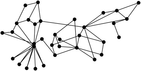
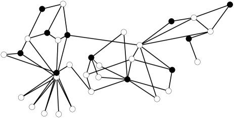
  Figure 1.

• The set of nodes for a structure subgraph consists of a focus node and all nodes that are at a graph distance $1$ or $2$ to it, which might include, of course, also other foci nodes. The set of edges is then formed as all edges from the original graph that connect the nodes belonging to the structure subgraph.

  Figures 2–7 show the structure subgraphs for our example. We have found a maximal independent set consisting of $11$ nodes and therefore we have formed $11$ subgraphs.

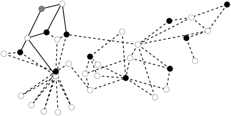
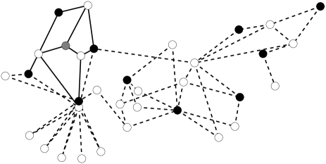
  Figure 2.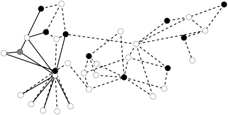

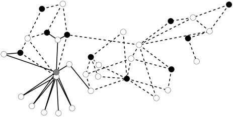
  Figure 3.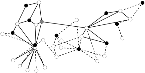

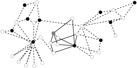
  Figure 4.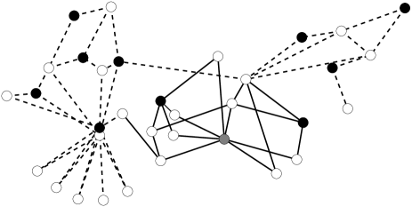

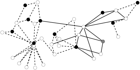
  Figure 5.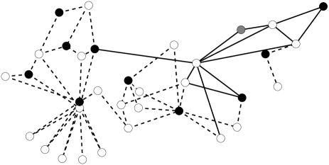

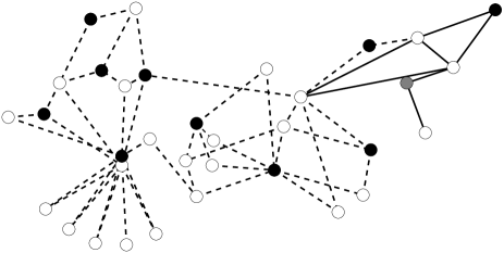
  Figure 6.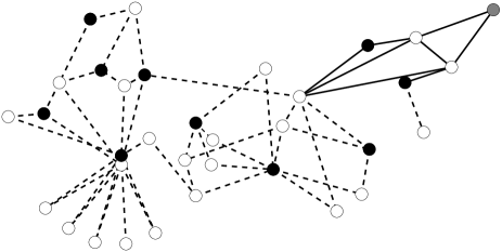

  

  Figure 7.

• We construct a ”coarser subgraph” $K^{1}$ from the original graph. Its nodes are the nodes from $\mathcal{V}^{1}$ and two nodes are connected by an edge in $K^{1}$ if in the original graph they are at a graph distance $2$. Note that by definition this is the smallest graph distance at which any nodes from $\mathcal{V}^{1}$ could be in $K$.

• We find a maximal independent set of nodes in the ”coarser subgraph” and denote it by $\mathcal{V}^{2}$. Each of the nodes in $\mathcal{V}^{2}$ will play the role of a ”focus” of a macrostructure subgraph and would specify this subgraph.

  Step III and Step IV of the procedure are represented on Figure 8 in a similar way as in Figure 1. This time the maximal independent subset consists of the $5$ nodes depicted in black on the right subfigure.

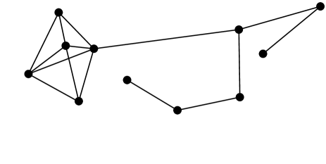
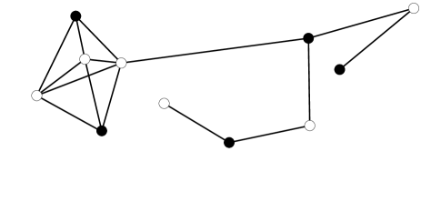
  Figure 8.

• We construct a macrostructure subgraph for each node from $\mathcal{V}^{2}$ by assembling all structure subgraphs whose focal nodes are at a graph distance smaller or equal to $1$ in $K^{1}$.

  This step is illustrated in Fig. 9–Fig. 13. On the top subfigures the macrostructure subgraphs are depicted with solid lines within the original graph, on the lower left subfigure for clarity they are displayed by themselves. The lower right subfigures show only these nodes from the macrostructure subgraphs that belong to the MIS and two nodes have been connected by an edge under the condition that there has been a path between them in the macrostructure subgraph consisting only of nodes that are not in $\mathcal{V}^{1}$.

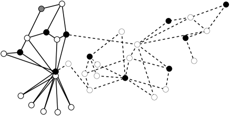
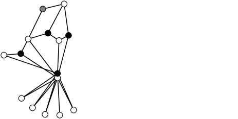
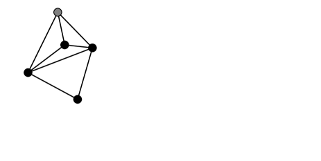
  Figure 9.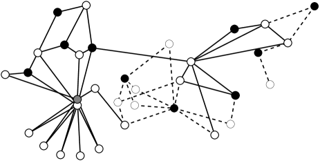

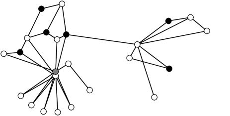
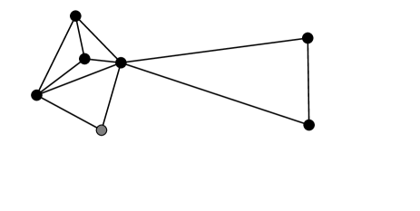
  Figure 10.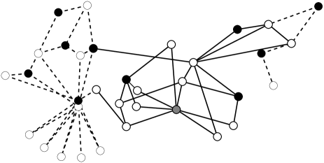

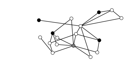
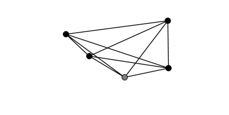
  Figure 11.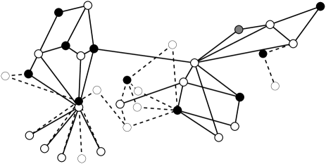

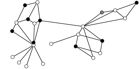
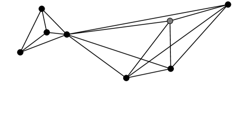
  Figure 12.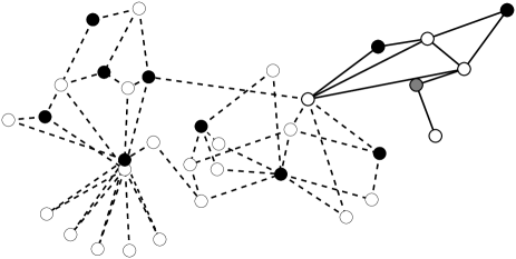

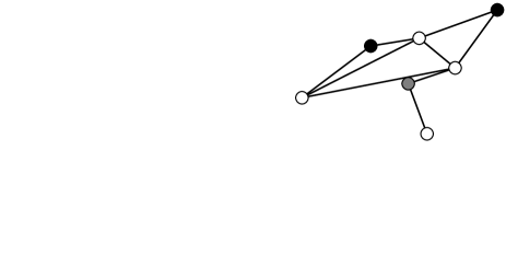
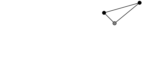
  Figure 13.

There are $3$ remarks to be made regarding the defined procedure:

Remark 2.3.

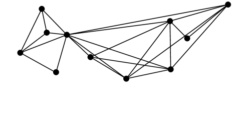
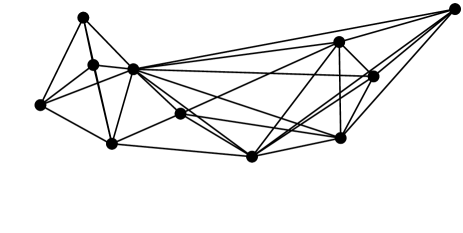
The very last step in the procedure implicates the construction of two coarse graphs with nodes belonging only to $\mathcal{V}^{1}$. The first one shown on the left of Figure 14 is the graph assembled from all graphs depicted in the lower right subfigures of Fig. 9–Fig. 13. In the second graph illustrated on the right of Figure 14 two nodes are adjacent if there is a path between them in the original graph $K$ consisting only of nodes that are not in $\mathcal{V}^{1}$. Note that the graph on the right of Fig. 14 is the adjacency graph of the global Schur complement which results from eliminating all nodes that do not belong to $\mathcal{V}^{1}$.

As one could observe, the left graph has a sparser structure than the right one and this difference will be much more pronounced on bigger graphs when the size of the macrostructures is small as compared to the size of the entire graph.

Figure 14.

Remark 2.4.

The described procedure fulfils the requirements defined in (2) and the coarser graph $K^{1}$ is connected. These statements are left as a remark as their proof is evident.

Remark 2.5.

There are also other ways to construct the coverings $\mathcal{G}$ and $\mathcal{F}$ of $K$. For example, in Step V one could choose the graph distance according to which the macrostructure subgraphs are assembled to be $2$ instead of $1$. It is possible to apply other assembling conditions and restrictions so long as condition (2) is fulfilled.

3. Auxiliary space multigrid (ASMG)

In matrix notation the above described procedure represents the following algorithm:

Algorithm 3.1.

  Additive Schur Complement Approximation (ASCA):  

1. Starting with a global two-level splitting of the degrees of freedom $\mathcal{D}$ into “coarse” ($\mathcal{D}_{c}$) and “fine” ($\mathcal{D}_{f}$), that is

   $$\mathcal{D}=\mathcal{D}_{c}\oplus\mathcal{D}_{f},$$

   find a covering $\mathcal{G}$ of $\mathcal{F}$ and a set of scaling factors $\{\sigma_{F,G}\}$.

2. For all $K_{G}\in\mathcal{G}$ execute the following steps:

   • Fix the “local” two-level numbering of DOF of $K_{G}$ to obtain

     $$A_{G}=\left[\begin{array}[]{cc}A_{G:11}&A_{G:12}\\[5.69054pt] A_{G:21}&A_{G:22}\end{array}\right]\begin{array}[]{l}\}\ \mathcal{D}_{G:c}\\[5.69054pt] \}\ \mathcal{D}_{G:f}\end{array}$$

   • Compute the “local” Schur complement $S_{G}=A_{G:11}-A_{G:12}A_{G:22}^{-1}A_{G:21}.$

   • Determine the “local-to-global” mapping $R_{G:1}=R_{G:c}$ for the CDOF in $\mathcal{D}_{G:c}$.

3. Compose the global Schur complement approximation $Q$ from “local” exact Schur complements $S_{G}$, i.e.,

   $$Q=\sum_{K_{G}\in\mathcal{G}}R_{G:c}^{T}S_{G}R_{G:c}=\sum_{K_{G}\in\mathcal{G}}R_{G:1}^{T}S_{G}R_{G:1}.$$

   Here the operators $R_{G:c}$ map a global vector from the space defined by $K^{1}$ to the local spaces related to the CDOF in the subgraphs $K_{G}$.

 

Remark 3.2.

In the ASCA algorithm the degrees of freedom $\mathcal{D}$ are vertex degrees of freedom and the two-level splitting $\mathcal{D}=\mathcal{D}_{f}\oplus\mathcal{D}_{c}$ is defined in Step I from the previous section.

Let $n_{1}:=|\mathcal{D}_{\rm c}|$, $n_{2}:=|\mathcal{D}_{\rm f}|$ be the cardinalities of $\mathcal{D}_{\rm c}$ and $\mathcal{D}_{\rm f}$. We denote with $n_{G:1}$, $n_{G:2}$ the number of CDOF and FDOF associated with $K_{G}$, i.e. $n_{G}=n_{G:1}+n_{G:2}$ where $\dim(V_{G})=n_{G}$.

We introduce the auxiliary space $\widetilde{V}$ of size $\tilde{n}=n_{1}+(\sum_{i=1}^{n_{\mathcal{G}}}n_{G_{i}:2})$ and a surjective mapping $\Pi:\widetilde{V}\rightarrow V$. The inclusion mapping $R^{T}:V\rightarrow\widetilde{V}$ has the form:

$$R^{T}=\left[\begin{array}[]{cc}I_{1}&0\\ 0&R_{2}^{T}\end{array}\right],\qquad\text{where}\qquad R_{2}^{T}=\left[\begin{array}[]{c}R_{1:2}\\ R_{2:2}\\ \vdots\\ R_{n_{\mathcal{G}}:2}\end{array}\right]\in\mathbb{R}^{n_{1}\times\left(\sum_{i=1}^{n_{\mathcal{G}}}n_{G_{i}:2}\right)}.$$

The matrix

$$\widetilde{A}:=\left[\begin{array}[]{cc}\widetilde{A}_{11}&\widetilde{A}_{12}\\ \widetilde{A}_{21}&\widetilde{A}_{22}\end{array}\right]$$

with blocks

$$\widetilde{A}_{11}:=\sum_{i=1}^{n_{\mathcal{G}}}R^{T}_{i:1}A_{G_{i}:11}R_{i:1},\qquad\widetilde{A}_{22}:=\left[\begin{array}[]{cccc}A_{G_{1}:22}&&&\\[2.15277pt] &A_{G_{2}:22}&&\\[2.15277pt] &&\ddots&\\[2.15277pt] &&&A_{G_{n_{\mathcal{G}}}:22}\\[2.15277pt] \end{array}\right],$$

$$\widetilde{A}_{12}:=[R_{1:1}^{T}A_{G_{1}:12},R_{2:1}^{T}A_{G_{2}:12},\ldots,R^{T}_{n_{\mathcal{G}}:1}A_{G_{n_{\mathcal{G}}}:12}],$$

$$\widetilde{A}_{21}:=[R_{1:1}^{T}A_{G_{1}:12},R_{2:1}^{T}A_{G_{2}:12},\ldots,R^{T}_{n_{\mathcal{G}}:1}A_{G_{n_{\mathcal{G}}}:12}]^{T}$$

is SPSD and defines an energy inner product on the auxiliary space $\widetilde{V}$. It is evident that $A=R\widetilde{A}R^{T}$ and $\widetilde{A}_{22}$ is a block-diagonal matrix whose blocks are of size $n_{G_{i}:2}{\times}n_{G_{i}:2}$ for $i=1,2,\ldots,n_{\mathcal{G}}$.

3.1. Auxiliary space method

3.1.1. Two-grid preconditioner

The auxiliary space preconditioner $C$ of $A$, see e.g. [17, 19], is defined as

(4) $$C^{-1}=\Pi_{\widetilde{D}}\widetilde{A}^{-1}\Pi^{T}_{\widetilde{D}},$$

where the surjective mapping $\Pi_{\widetilde{D}}:\widetilde{V}\rightarrow V$ is given by

(5) $$\Pi_{\widetilde{D}}=(R\widetilde{D}R^{T})^{-1}R\widetilde{D}\qquad\text{and}\qquad\widetilde{D}=\left[\begin{array}[]{cc}I&0\\ 0&\widetilde{D}_{22}\end{array}\right].$$

The preconditioner (4) can be further generalized, see e.g. [23], as

(6) $$B^{-1}:=\overline{M}^{-1}+(I-M^{-T}A)C^{-1}(I-AM^{-1}),$$

see e.g. [19], where $C$ is given by (4), $M$ is an $A$-norm convergent smoother and $\overline{M}=M(M+M^{T}-A)^{-1}M^{T}$ is the corresponding symmetrised smoother. Results related to the condition number estimate of $B^{-1}A$ can be found in [17].

Remark 3.3.

Different choices for $\widetilde{D}_{22}$ in (5) are possible, for example $\widetilde{D}_{22}=\widetilde{A}_{22}$, $\widetilde{D}_{22}={\rm diag}(\widetilde{A}_{22})$ or $\widetilde{D}_{22}={\rm tridiag}(\widetilde{A}_{22})$. Discussion about the effect of these choices on the convergence and complexity of the method can be found in [17].

3.1.2. Multigrid precondtioner

The procedure in Section 2.2 can be recursively applied thus resulting in the construction of the nested spaces $\mathcal{V}^{\ell}\subset\ldots\subset\mathcal{V}^{0}=\mathcal{V}$ related to the graphs $K_{\ell}=(\mathcal{V}^{\ell},\mathcal{E}^{\ell}),\ldots,K_{0}=K=(\mathcal{V},\mathcal{E})$. Then

$$A^{(0)}:=A$$

denotes the Laplacian matrix for the original graph $K$. Let the index $k$ be in $\{0,\ldots,\ell-1\}$ and consider the sequence of auxiliary space matrices $\widetilde{A}^{(k)}$ in the two-by-two block factorised form

(7) $$({\widetilde{A}}^{(k)})^{-1}=(\widetilde{L}^{(k)})^{T}\widetilde{D}^{(k)}\widetilde{L}^{(k)},$$

where

$$\widetilde{L}^{(k)}=\left[\begin{array}[]{cc}I&-\widetilde{A}^{(k)}_{12}(\widetilde{A}^{(k)}_{22})^{-1}\\ &I\end{array}\right]\qquad\text{and}\qquad\widetilde{D}^{(k)}=\left[\begin{array}[]{cc}{Q^{(k)}}^{-1}&\\ &(\widetilde{A}^{(k)}_{22})^{-1}\end{array}\right].$$

The next coarser level matrix $A^{(k+1)}$ is defined through the additive Schur complement approximation $Q^{(k)}$, i.e.

(8) $$A^{(k+1)}:=Q^{(k)}.$$

The (nonlinear) AMLI-cycle ASMG preconditioner $C^{(k)}$ at level $k$ has the form

(9) $${C^{(k)}}^{-1}:=\Pi^{(k)}(\widetilde{L}^{(k)})^{T}\left[\begin{array}[]{cc}C_{\nu}^{(k+1)}&\\ &\widetilde{A}^{(k)}_{22}\end{array}\right]^{-1}\widetilde{L}^{(k)}{\Pi^{(k)}}^{T}.$$

Here $\left[C_{\nu}^{(k+1)}\right]^{-1}$ is an approximation of the inverse of $A^{(k+1)}$ where at the coarsest level we set

(10) $$\left[C_{\nu}^{(\ell)}\right]^{-1}:={A^{(\ell)}}^{-1}$$

while for $k<\ell-1$ a matrix polynomial of the form

(11) $$\left[C_{\nu}^{(k+1)}\right]^{-1}:=(I-p^{(k)}({C^{(k+1)}}^{-1}A^{(k+1)})){A^{(k+1)}}^{-1}$$

is used to determine $\left[C_{\nu}^{(k+1)}\right]^{-1}$.

The incorporation of pre- and post-smoothing results in the following AMLI-cycle ASMG preconditioner:

(12) $${B^{(k)}}^{-1}:={\overline{M}^{(k)}}^{-1}+(I-{M^{(k)}}^{-T}A^{(k)})\Pi^{(k)}(\widetilde{L}^{(k)})^{T}{\overline{D}^{(k)}}^{-1}\widetilde{L}^{(k)}{\Pi^{(k)}}^{T}(I-A^{(k)}{M^{(k)}}^{-1}),$$

where

$$\quad\overline{D}^{(k)}:=\left[\begin{array}[]{cc}B_{\nu}^{(k+1)}&\\ &\widetilde{A}^{(k)}_{22}\end{array}\right]\quad\text{and}\quad\left[B_{\nu}^{(k+1)}\right]^{-1}=q^{(k)}({B^{(k+1)}}^{-1}A^{(k+1)})){B^{(k+1)}}^{-1}.$$

We write $[B_{\nu}^{(k+1)}]^{-1}$ as $B_{\nu}^{(k+1)}[\cdot]$ (and $[C_{\nu}^{(k+1)}]^{-1}$ as $C_{\nu}^{(k+1)}[\cdot])$) to denote that for the nonlinear AMLI-cycle ASMG method the coarse-level preconditioner is a nonlinear mapping whose action on a vector d is realised by $\nu$ iterations with a preconditioned Krylov subspace method. In what follows, we employ the generalised conjugate gradient method and hence denote $B_{\nu}^{(k+1)}[\cdot]\equiv B^{(k+1)}_{\text{GCG}}[\cdot]$ (and $C_{\nu}^{(k+1)}[\cdot]\equiv C^{(k+1)}_{\text{GCG}}[\cdot]$).

Remark 3.4.

The method of auxiliary space preconditioning dates back to the works of Matsokin and Nepomnyashchikh, see  [24, 25, 26].

When applied recursively, the procedure in Section 2.2 generates sequences of macrostructure and structure subgraphs fitted to the multilevel splitting of the DOF. It is clear that the focus node of a macrostructure subgraph will always be a focus node of a structure subgraph on the next coarser level. However, not all possible ways of defining the structures, macrostructures and the adjacency pattern of the coarser graph in Step II, Step IV and Step III respectively will be consistent in the sense that the coarse nodes in a given macrostructure coincide with the nodes of the corresponding structure on the next coarser level.

One simple strategy to avoid such inconsistency is to run the described procedure recursively only to generate the multilevel splitting of the DOF and the macrostructure-structure relation needed in (3). To generate the structures on the finest level one could apply a rule, as in Step II of the procedure, and then use the obtained structures in the assembly of the finest level macrostructures. On all coarser levels the structures could then directly be associated with adjacency graphs of the local Schur complement matrices computed in Step 2(b) of Algorithm 3.1, cf. also with (8).

It is worth mentioning that this problem of inconsistency does not appear for the particular choice of defining the structures, macrostructures and coarse subgraphs presented in the description of the procedure in Section 2.2. As it is easy to be seen, in this particular setting the coarse vertices that a macrostructure subgraph contains are either at a graph distance $2$ or $4$ to the focus node in the original graph $K$ and in the coarser graph $K^{1}$ exactly these and no other coarse nodes are at a graph distance $1$ or $2$ to this node.

4. Complexity of the ASMG preconditioner

The computational complexity of the ASMG preconditioner relates directly to the work spent on constructing the precondtioner and work for its utilization. The work is determined by the number of arithmetic operations which is mainly affected by the sparsity of the involved matrices. For that reason in what follows we want to comment on the sparsity of the coarse-level matrices generated by Algorithm 3.1.

Let $\mathcal{S}$ be the set containing the undirected unweighted graphs $K_{S_{G}}=(\mathcal{V}_{S_{G}},\mathcal{E}_{S_{G}})$ corresponding to the adjacency matrices of the local Schur complements $S_{G}$ as computed in Step 2 (b) in the algorithm. Here $\mathcal{V}_{S_{G}}$ and $\mathcal{E}_{S_{G}}$ designate respectively the set of vertices and the set of edges. Obviously, $\mathcal{V}_{S_{G}}\subset\mathcal{V}_{G}$, however, $\mathcal{E}_{S_{G}}$ is not a subset of $\mathcal{E}_{G}$. Frequently but not always, $K_{S_{G}}$ will be a so-called clique, i.e., a graph in which every pair of distinct vertices (DOF) is connected by an edge.

Now, let the coarse-level matrix $A^{(k+1)}$ be defined via (8) where $Q^{(k)}=Q$ results from ASCA, i.e., from Algorithm 3.1, Step 3. The following lemma characterizes the sparsity pattern of the coarse-level matrix $Q$.

Lemma 4.1.

Let

$$Q=(q_{ij})_{i,j=1}^{|\mathcal{D}_{c}|}=\sum_{K_{G}\in\mathcal{G}}R_{G:1}^{T}S_{G}R_{G:1}.$$

The entry $q_{ij}$ of $Q$ is zero for any pair of coarse DOF $d_{i}$, $d_{j}\in\mathcal{D}_{c}$ if there does not exist a graph $K_{S_{G}}\in\mathcal{S}$ for which both $d_{i}$ and $d_{j}$ are in $\mathcal{V}_{S_{G}}\;(\equiv\mathcal{D}_{G:c})$.

Proof.

Assume that

$$q_{ij}=\sum_{K_{G}\in\mathcal{G}}\langle S_{G}R_{G:1}\,{\text{{e}}}_{i},R_{G:1}\,{\text{{e}}}_{j}\rangle\neq 0,$$

where ${\text{{e}}}_{i}$ and ${\text{{e}}}_{j}$ denote the $i$-th and $j$-th canonical basis vectors in $\mathbb{R}^{|\mathcal{D}_{c}|}$, respectively. Then there exists $K_{G}$ for which $\langle S_{G}R_{G:1}\,{\text{{e}}}_{i},R_{G:1}\,{\text{{e}}}_{j}\rangle={\text{{e}}}_{j}^{T}R_{G:1}^{T}S_{G}R_{G:1}\,{\text{{e}}}_{i}\neq 0$.

Hence, from the identity ${\text{{e}}}_{j}^{T}R_{G:1}^{T}S_{G}R_{G:1}\,{\text{{e}}}_{i}=\lambda(S_{G}R_{G:1}\,{\text{{e}}}_{i}{\text{{e}}}_{j}^{T}R_{G:1}^{T})$, where $\lambda(M)$ denotes the largest-in-magnitude eigenvalue of any square real matrix $M$, it follows that the rank one matrix $R_{G:1}{\text{{e}}}_{i}{\text{{e}}}_{j}^{T}R_{G:1}^{T}$ has to be different from the matrix of all zeros. In view of the definition of $R_{G:1}$ the condition $d_{i}$ and $d_{j}$ not both belonging to $\mathcal{D}_{G:1}$, however, implies that $R_{G:1}\,{\text{{e}}}_{i}{\text{{e}}}_{j}^{T}R_{G:1}^{T}=0$ which is a contradiction. ∎

The next lemma gives conditions which control the sparsity of the Schur complement approximation $Q$.

Lemma 4.2.

Let $(\widetilde{\mathcal{V}},\widetilde{\mathcal{E}})$ be the the (factor) graph representing the adjacency of the graphs belonging to $\mathcal{S}$, defined by identifying each graph $K_{S_{G}}=(\mathcal{V}_{S_{G}},\mathcal{E}_{S_{G}})$ with a vertex $v_{G}\in\widetilde{\mathcal{V}}$ and connecting two vertices $v_{G^{\prime}}$ and $v_{G^{\prime\prime}}$ by an edge ${\text{{e}}}_{{G^{\prime}}{G^{\prime\prime}}}\in\widetilde{\mathcal{E}}$ if and only if $\mathcal{V}_{S_{G^{\prime}}}\cap\mathcal{V}_{S_{G^{\prime\prime}}}\neq\emptyset$.

Under the assumptions that

• $(\widetilde{\mathcal{V}},\widetilde{\mathcal{E}})$ has a bounded vertex degree, i.e., $degree(v_{G})\leq c_{1}$ for all $v_{G}\in\widetilde{\mathcal{V}}$,

and

• the size of the graphs $K_{S_{G}}$ is uniformly bounded, i.e., $|\mathcal{V}_{S_{G}}|\leq c_{2}$ for all $K_{G}\in\mathcal{G}$,

the coarse-level matrix $Q$ is sparse, i.e., the number of non-zero entries in every row of $Q$ is bounded by a constant $c_{3}$.

Proof.

Due to property (i) for a given row $k$ the degree of freedom $d_{k}\in\mathcal{D}_{c}$ can belong to at most $(c_{1}+1)$ graphs $K_{S_{G}}$. Because of Lemma 4.1 a non-zero entry $q_{km}\neq 0$ can only occur if there exists $K_{S_{G}}$ such that both $d_{k}$ and $d_{m}$ belong to $\mathcal{V}_{S_{G}}$. However, since there are at most $(c_{1}+1)$ such possibilities and the size of the corresponding graphs is bounded by $c_{2}$, see assumption (ii), the total number of non-zero entries in row $k$ is bounded by $c_{3}:=(c_{1}+1)(c_{2}-1)+1$. ∎

Discussion about the complexity of the ASMG algorithm based on ASCA can also be found in [23].

5. Numerical tests

The convergence performance of the AMLI-cycle ASMG method based on ASCA is shown in $8$ examples from

http://www.cise.ufl.edu/research/sparse/matrices/list_by_id.html,

see [27], also [28, 29] and Figures LABEL:Fig15–LABEL:Fig22. In Tables 1–8 additionally to the number of iterations we report the number of CDOF for all levels.

The numerical experiments have been run for:

• V- and W-cycles;

• $2$ Gauss-Seidel smoothing steps;

• a random start vector;

• zero right hand side;

• stopping criterium: relative residual $10^{-8}$;

• final level of coarsening: number of CDOF $\leq 40$.

For Examples 1–4, 6–8 the components of the ASMG method based on ASCA are constructed in accordance with the procedure in Section 2.2 whereas in Example 5, where the graph is very sparse, we have chosen in Step II of the procedure the set of nodes that defines a structure subgraph to consist of a focus node and all nodes that are at a graph distance $1$, $2$, $3$ or $4$ to it.

Example 1

In this example the graph consists of $7\,928$ nodes and $59\,379$ edges. The minimum vertex degree is $1$, the maximum vertex degree is $33$, the average vertex degree is $\approx 14,98$.

Description	skirt, with coordinates. From NASA, collected by Alex Pothen
Author	NASA
Editor	G. Kumfert A. Pothen

Levels	2	3	4	5
V-cycle	17	17	18	18
W-cycle	17	17	17	17
CDOF	2422	608	137	40

Table 1. Example 1, $7\,928$ DOF

Example 2

Here, there are $10\,429$ nodes, $46\,585$ edges and the minimum vertex degree is $3$, the maximum vertex degree is $27$ and the average vertex degree is $\approx 8,93$.

Description	SHUTTLE_EDDY: Nasa matrix, but with diagonal added to original matrix
Author	NASA
Editor	G. Kumfert A. Pothen

Levels	2	3	4	5
V-cycle	10	11	12	13
W-cycle	10	10	10	10
CDOF	1411	333	106	37

Table 2. Example 2, $10\,429$ DOF

Example 3

For the graph $K=(\mathcal{V},\mathcal{E})$ considered in this example we have $|\mathcal{V}|=16\,146$ and $|\mathcal{E}|=499\,505$. $89$ is the highest vertex degree whereas the minimum and the average are $24$ and $\approx 61,87$ respectively.

Description	STRUCTURE FROM NASA LANGLEY, ACCURACY PROBLEM ON Y-MP
Author	H. Simon
Editor	H. Simon

Levels	2	3	4	5
V-cycle	12	14	14	14
W-cycle	12	12	12	12
CDOF	643	143	49	13

Table 3. Example 3, $16\,146$ DOF

Example 4

The graph presented in Example 4 has $67\,578$ nodes and $168\,176$ edges. Here the highest vertex degree is $53$, the minimum $1$ and the average $\approx 4,98$.

Description	DIMACS10 set: redistrict/ct2010 and ct2010a
Author	W. Zhao
Editor	H. Meyerhenke

Levels	2	3	4	5	6	7
V-cycle	-	13	14	16	17	17
W-cycle	-	10	10	10	10	10
CDOF	22714	5267	1497	425	123	39

Table 4. Example 4, $67\,578$ DOF

Example 5

In this Example the graph consists of $126\,146$ nodes and $161\,950$ edges. The maximum vertex degree is $7$, the minimum $1$ and the average $\approx 2,57$.

Description	Continental US road network (with $xy$ coordinates
Author	D. Gleich
Editor	T. Davis

Levels	2	3	4	5	6	7	8	9	10
V-cycle	-	-	-	14	16	18	19	20	20
W-cycle	-	-	-	7	7	7	7	7	7
CDOF	57018	21671	8703	3253	1201	430	152	51	15

Table 5. Example 5, $126\,146$ DOF

Example 6

The graph in Example 6 has $143\,437$ nodes, $409\,593$ edges, maximum vertex degree $6$, minimum vertex degree $2$ and average vertex degree $\approx 5,71$.

Description	DIMACS10 set: walshaw/fe_ocean
Author	F. Pellegrini
Editor	C. Walshaw

Levels	2	3	4	5	6	7
V-cycle	12	13	15	15	15	15
W-cycle	12	13	13	13	13	13
CDOF	71386	10026	1927	414	100	31

Table 6. Example 6: $143\,437$ DOF

Example 7

Example 7 considers a graph with $214\,765$ nodes, $1\,679\,018$ edges. The maximum, minimum and average vertex degrees are $40$, $4$ and $\approx 15,64$ respectively.

Description	DIMACS10 set: walshaw/m14b
Author	V. Kumar
Editor	C. Walshaw

Levels	2	3	4	5	6	7
V-cycle	-	10	12	13	13	13
W-cycle	-	8	8	8	8	8
CDOF	30238	5634	1990	288	69	16

Table 7. Example 7: $214\,765$ DOF

Example 8

The graph in Example 8 has $1\,048\,572$ nodes and $6\,891\,617$ edges. Its maximum vertex degree is $32$, its minimum $1$ and average $\approx 13,14$.

Description	DIMACS10 set: random/rgg_n_2_20_s0
Author	M. Holtgrewe P. Sanders C. Schulz
Editor	C. Schulz

Levels	2	3	4	5	6	7	8	9	10
V-cycle	-	-	-	16	18	19	19	19	19
W-cycle	-	-	-	11	11	11	11	11	11
CDOF	160410	48818	15966	5249	1729	586	208	68	23

Table 8. Example 8: $1\,048\,572$ DOF

Remark 5.1.

We have implemented both the deflated CG method and the rank-$1$ update of the graph Laplacian matrix and as one would expect we have observed the same number of iterations in both cases.

Remark 5.2.

In Tables 5–8 we report the number of iterations only for the $\ell$-level methods with CDOF $\leq 10\,000$ as solving exactly such big problems is time and memory consuming.

6. Conclusions

The approach of the auxiliary space multigrid preconditioning based on ASCA as recently presented in [17] has been successfully extended to graph Laplacian matrices for general unstructured graphs. We have suggested a procedure and an algorithm to set up a hierarchy of coarse-grid operators that results in fast multigrid convergence. The operator complexity can be controlled by the size of the building components, see the discussion in Section 4.

We have numerically tested the proposed approach on several examples. As can be seen from the results in Tables 1–8 the W-cycle converges uniformly in the number of levels, whereas for Examples 1, 3, 6–8 we observe also a uniformly convergent V-cycle.

After all, it is still worth mentioning that the approach is purely algebraic and easy to be implemented from an algorithmic point of view. Furthermore, there are no limitations regarding the topology of the graphs.

Future work will address weighted graph Laplacian systems.

References

- [1] M. Belkin, P. Niyogi, and V. Sindhwani. Manifold regularization: A geometric framework for learning from labeled and unlabeled examples. J. Mach. Learn. Res., 7:2399–2434, 2006.
- [2] T. Joachims. Transductive learning via spectral graph partitioning. In T. Fawcett and N. Mishra, editors, ICML’03 Proceedings of the Twentieth International Conference on International Conference on Machine Learning, pages 290–297, 2003.
- [3] U. von Luxburg. A tutorial on spectral clustering. Stat. Comput., 17:395–416, 2007.
- [4] Z. Qi, Y. Tian, and Y. Shi. Laplacian twin support vector machine for semi-supervised classification. Neural Netw., 35:46–53, 2012.
- [5] X. Zhu, J. Lafferty, and Z. Ghahraman. Combining active learning and semi-supervised learning using gaussian fields and harmonic functions. In ICML 2003 Workshop on the Continuum from Labeled to Unlabeled Data in Machine Learning and Data Mining, pages 58–65, 2003.
- [6] D. Spielman. Algorithms, graph theory, and linear equations in laplacian matrices. In Proceedings of the International Congress of Mathematicians 2010 (ICM 2010), World Scientific, pages 2698–2722, 2010.
- [7] O. E. Livne and A. E. Brandt. Lean algebraic multigrid (LAMG): Fast graph Laplacian linear solver. SIAM J. Sci. Comput., 34:B499–B522, 2012.
- [8] J. Brannick, Y. Chen, J. Kraus, and L. Zikatanov. Algebraic multilevel preconditioners for the graph laplacian based on matching in graphs. SIAM J. Numer. Anal., 51:1805–1827, 2013.
- [9] J. Brannick. Aggregation-based aggressive coarsening with polynomial smoothing. In J. Erhel, M. J.. Gander, L. Halpern, G. Pichot, T. Sassi, and O. Widlund, editors, Domain Decomposition Methods in Science and Engineering XXI, Lecture Notes in Computational Science and Engineering, pages 285–293. Springer, 2014.
- [10] A. Napov and Y. Notay. An efficient multigrid method for graph laplacian systems. Electron. Trans. Numer. Anal., 45:201–218, 2016.
- [11] Compatible matching adaptive amg preconditioners for laplacian matrices on general graphs, author = DflAmbra, P. and Vassilevski, P., year = 2015, institution = Lawrence Livermore National Laboratory, date-added = 2017-08-08 17:45:43 +0000. Technical report.
- [12] P. DellflAcqua, A. Frangioni, and S. Serra-Capizzano. Accelerated multigrid for graph laplacian operators. Appl. Math.Comput., 270:193–215, 2015.
- [13] I. Koutis and G. L. Miller. Combinatorial preconditioners and multilevel solvers for problems in computer vision and image processing. In J. Erhel, M. J.. Gander, L. Halpern, G. Pichot, T. Sassi, and O. Widlund, editors, Proceedings of the 5th International Symposium on Advances in Visual Computing: Part I, Lecture Notes in Computational Science and Engineering, pages 1067–1078, Berlin, 2009. Springer-Verlag.
- [14] I. Koutis. Combinatorial and Algebraic Tools for Optimal Multilevel Algorithms. PhD thesis, Carnegie Mellon University, Pittsburgh, PA, 2007.
- [15] N. K. Vishnoi. Laplacian Solvers and Their Algorithmic Applications, volume 8 of Foundations and Trends in Theoretical Computer Science. Now Publishers Inc, 2012.
- [16] J. Kraus. Additive schur complement approximation and application to multilevel preconditioning. SIAM J. Sci. Comput., 34:A2872–A2895, 2012.
- [17] J. Kraus, M. Lymbery, and S. Margenov. Auxiliary space multigrid method based on additive Schur complement approximation. Numer. Linear Algebra Appl., 22:965–986, 2015.
- [18] R. Hiptmair and J. Xu. Nodal auxiliary space preconditioning in h(curl) and h(div) spaces. SIAM J. Numer. Anal., 45:2483–2509, 2007.
- [19] J. Xu. The auxiliary space method and optimal multigrid preconditioning techniques for unstructured grids. Computing, 56:215–235, 1996.
- [20] D. M. Alber and L. N. Olson. Coarsening invariance and bucket-sorted independent sets for algebraic multigrid. Electron. Trans. Numer. Anal., 37:367–385, 2010.
- [21] I. Moulitsas and G. Karypis. Multilevel algorithms for generating coarse grids for multigrid methods. In Proceedings of the 2001 ACM/IEEE conference on Supercomputing, pages 45–45, 2001.
- [22] Y. Saad, M. Yeung, J. Erhel, and F. Guyomarc’h. Preconditioning heterogeneous H(div) problems by additive Schur complement approximation and applications. SIAM J. Sci. Comput., 21:1909–1926, 2006.
- [23] J. Kraus, R. Lazarov, M. Lymbery, S. Margenov, and L. Zikatanov. Preconditioning heterogeneous H(div) problems by additive Schur complement approximation and applications. SIAM J. Sci. Comput., 38:A875–A898, 2016.
- [24] A. Matsokin and S. Nepomnyashchikh. The schwarz alternation method in a subspace. IIzv. Vyssh. Uchebn. Zaved. Mat., 10:61–66, 1985.
- [25] S. Nepomnyaschikh. Mesh theorems on traces, normalizations of function traces and their inversion. Soviet J. Numer. Anal. Math. Modelling, 3:223–242, 1991.
- [26] S. Nepomnyaschikh. Fictitious space method on unstructured meshes. East-West J. Numer. Math., 1:71–79, 1995.
- [27] T. A. Davis and Y. Hu. The university of florida sparse matrix collection. ACM Trans. Math. Softw., 38:1–25, 2011.
- [28] Graph partitioning and graph clustering. In D. A. Bader, H. Meyerhenke, P. Sanders, and D. Wagner, editors, 10th DIMACS Implementation Challenge Workshop. February 13–14, 2012, Lecture Notes in Computational Science and Engineering, pages 285–293, Georgia Institute of Technology, Atlanta, GA, 2013. Springer.
- [29] I. S. Duff, R. G. Grimes, and J. G. Lewis. Sparse matrix test problems. ACM Trans. Math. Softw., 15:1 – 14, 1989.