Threshold resummation of the rapidity distribution for Higgs production at NNLO+NNLL

Abstract

We present a formalism that resums threshold-enhanced logarithms to all orders in perturbative QCD for the rapidity distribution of any colorless particle produced in hadron colliders. We achieve this by exploiting the factorization properties and K+G equations satisfied by the soft and virtual parts of the cross section. We compute for the first time compact and most general expressions in two-dimensional Mellin space for the resummed coefficients. Using various state-of-the-art multiloop and multileg results, we demonstrate the numerical impact of our resummed results up to next-to-next-to-leading order for the rapidity distribution of the Higgs boson at the LHC. We find that inclusion of these threshold logs through resummation improves the reliability of perturbative predictions.

This article is dedicated to the memory of Jack Smith.

Introduction.—With the successful running of the LHC at CERN and precise theoretical predictions from various state-of-the-art computations, we can now test the Standard Model (SM) of particle physics with unprecedented accuracy and also severely constrain many physics beyond the SM (BSM) scenarios. The spectacular discovery Aad et al. (2012); *Chatrchyan:2012xdj of a scalar particle and the most precise prediction on its production cross section Anastasiou et al. (2015) improved our understanding of the symmetry-breaking mechanism, namely, the Higgs mechanism. The copious production of vector bosons $Z$s and $W^{\pm}$s and lepton pairs at the LHC through Drell-Yan (DY) process Drell and Yan (1970), which are used to precisely measure the parton distribution functions (PDFs) Gao et al. (2014); *Harland-Lang:2014zoa; *Ball:2014uwa; *Butterworth:2015oua; *Alekhin:2017kpj are also very important to study.

While inclusive rates are important for any phenomenological study, the differential cross sections often carry more information on the nature of interaction and quantum number of particles produced in the hard collisions. Rapidity distributions of Drell-Yan pair Khachatryan et al. (2015), $Z$ boson Affolder et al. (2001a), and charge asymmetries of leptons in $W^{\pm}$ boson decays Abe et al. (1998) are already used to measure PDFs. Possible excess events in these distributions can hint at BSM physics, namely, R-parity violating supersymmetric models Affolder et al. (2001b), models with $Z^{\prime}$ or with contact interactions, and large extra-dimension models Arkani-Hamed et al. (1998); *Randall:1999ee. Like in DY, measurements of transverse momentum and rapidity distributions of the Higgs boson will be very useful to study the properties of the Higgs boson and its couplings. Theoretical predictions for inclusive production Dawson (1991); *Djouadi:1991tka; *Spira:1995rr; *Harlander:2001is; *Catani:2001ic; *Harlander:2002wh; *Anastasiou:2002yz; *Ravindran:2003um; *KubarAndre:1978uy; *Altarelli:1978id; *Humpert:1980uv; *Matsuura:1987wt; *Matsuura:1988sm; *Hamberg:1990np as well as the rapidity distribution Anastasiou et al. (2003); *Anastasiou:2004xq of dileptons in DY production and the Higgs bosons in gluon-gluon fusion have been known to next-to-next-to-leading order (NNLO) in perturbative QCD for long time. A few years back, a complete next-to-next-to-next-to-leading-order (N³LO) prediction Anastasiou et al. (2015) for inclusive Higgs production became available after its soft-plus-virtual (SV) contributions (N³LO_SV) were computed in Ref. Anastasiou et al. (2014), see also Refs. Moch and Vogt (2005); *Laenen:2005uz; *Idilbi:2005ni; Ravindran (2006a, b) for earlier works and Ref. Kumar et al. (2015); *Ahmed:2014cha for Higgs productions in other channels at N³LO_SV and Ref. Ahmed et al. (2015a) for a renormalization group improved prediction to all orders for $gg\rightarrow H$. For DY, so far, only N³LO in the SV approximation is known Ahmed et al. (2014b), see also Ref. Li et al. (2014); *Catani:2014uta.

Both inclusive and differential cross sections are often plagued with large logarithms resulting from certain boundaries of the phase space, spoiling the reliability of the fixed-order predictions. In the inclusive case, this happens when partonic scaling variable $z=Q^{2}/\hat{s}\rightarrow 1$, i.e., threshold limit, resulting from the emission of soft gluons in the DY process ($Q^{2}=m_{l^{+}l^{-}}^{2}$) and in Higgs production ($Q^{2}=M_{H}^{2}$), where $m_{l^{+}l^{-}}$, $M_{H}$, and $\hat{s}$ are the invariant mass of the dileptons, the mass of the Higgs boson, and centre-of-mass energy squared of the partonic subprocess, respectively. One finds a similar problem when the transverse momentum of the final state becomes small. The resolution to this is to resum these large logs to all orders in perturbation theory. To achieve this, several approaches exist in the literature for both inclusive rates (see Refs. Sterman (1987); Catani and Trentadue (1989); *Catani:1990rp for the earliest approach) as well as for transverse momentum distributions Bozzi et al. (2008); *Bozzi:2008bb; *Bozzi:2010xn; *Catani:2010pd; *Catani:2013vaa; *Monni:2016ktx; *Ebert:2016gcn; *Grazzini:2015wpa; *Ferrera:2016prr. Catani and Trentadue, in their seminal work Catani and Trentadue (1989), demonstrated the resummation of leading large logs for the inclusive rates in Mellin space and extended their approach to a differential $x_{F}$ distribution using double Mellin moments. In the recent past, there have been several approaches to performing threshold resummation for rapidity distribution. In Ref. Laenen and Sterman (1992); *Sterman:2000pt; *Mukherjee:2006uu; *Bolzoni:2006ky, an appropriate Fourier transformation for the rapidity variable resums certain logs for the rapidity distribution, and in Ref. Becher and Neubert (2006); *Becher:2007ty; *Bonvini:2014qga, the authors have used soft-collinear effective theory (SCET) to identify the potential large logs that can be resummed (see also Ref. Ebert et al. (2017) for resumming timelike logarithms using SCET).

In Refs. Ravindran (2006a, b), one of the authors of the present article developed $z$-space formalism to obtain a soft distribution function that captures the threshold-enhanced part of the inclusive production of any colorless particle, using factorization properties of cross sections and K+G equations that the form factor as well as soft distribution function satisfy. In Ref. Ravindran (2006b), it was shown that the $N$th Mellin moment of the finite part of the universal soft distribution function was nothing but the threshold exponent á la Sterman Sterman (1987) and Catani and Trentadue Catani and Trentadue (1989, 1991). The same approach was later extended to obtain rapidity distributions of lepton pairs, Higgs boson Ravindran et al. (2007), and $Z$ and $W^{\pm}$ Ravindran and Smith (2007) using two scaling variables $z_{1}$ and $z_{2}$ in the threshold limit up to N³LO level Ahmed et al. (2014c); *Ahmed:2014era.

In this article, we derive an all-order resummed result in two-dimensional Mellin space for rapidity distribution of a colorless final state $F$ that can be produced in hadron colliders and present the numerical impact only for the production of the scalar Higgs boson at the LHC. We work with double Mellin variables $N_{1}$ and $N_{2}$ corresponding to $z_{1}$ and $z_{2}$ in $z$ space and demonstrate the resummation of large logarithms proportional to $\ln(N_{i})$ (in z space, these correspond to plus distributions in both the variables $z_{1}$ and $z_{2}$) in the limit $N_{i}\to\infty$ ($z_{i}\to 1$). Our approach, while it follows Ref. Catani and Trentadue (1989), differs from Refs. Sterman and Vogelsang (2001); Bolzoni (2006); Becher and Neubert (2006); Becher et al. (2008); Bonvini et al. (2015) in the way the threshold limits are defined. In the latter, resummation is done in Mellin-Fourier space spanned by $(N,M)$, which corresponds to the scaling variable $z$ and the partonic rapidity $y_{p}$. By taking the limit $N\to\infty$ and keeping $M$ fixed, the resummed result turns out to be identical to the inclusive one.

Theoretical framework.—The rapidity distribution of the state $F$ can be written as

$${d\sigma^{I}\over dy} = \sigma^{I}_{\rm B}(x_{1}^{0},x_{2}^{0},q^{2},\mu_{R}^{2})\sum_{ab=q,\overline{q},g}\int_{x_{1}^{0}}^{1}{dz_{1}\over z_{1}}\int_{x_{2}^{0}}^{1}{dz_{2}\over z_{2}}~{}$$ (1)

$$\!\!\times{\cal H}^{I}_{ab}\left({x_{1}^{0}\over z_{1}},{x_{2}^{0}\over z_{2}},\mu_{F}^{2}\right)\Delta^{I}_{d,ab}(z_{1},z_{2},q^{2},\mu_{F}^{2},\mu_{R}^{2}).$$

In the above, $\mu_{R}$ is the ultraviolet renormalization scale, the hadron level rapidity $y={1\over 2}\ln(p_{2}.q/p_{1}.q)={1\over 2}\ln\left({x_{1}^{0}/x_{2}^{0}}\right)$   and $\tau=q^{2}/S=x_{1}^{0}x_{2}^{0}$, $q$ being the momentum of the final state $F$, $S=(p_{1}+p_{2})^{2}$, where $p_{i}$ are the momenta of incoming hadrons $P_{i}~{}(i=1,2)$. For the DY process ($I=q$), the state $F$ is a pair of leptons with invariant mass $q^{2}$, $\sigma^{I}=d\sigma^{q}(\tau,q^{2},y)/dq^{2}$ whereas for the Higgs boson production through gluon (bottom-antibottom) fusion [$I=g(b)$], $\sigma^{I}=\sigma^{g(b)}(\tau,q^{2},y)$. The function ${\cal H}^{I}_{ab}$ in Eq.(1) is given by

$${\cal H}^{I}_{ab}(x_{1},x_{2},\mu_{F}^{2}) =f^{P_{1}}_{a}(x_{1},\mu_{F}^{2})~{}f^{P_{2}}_{b}(x_{2},\mu_{F}^{2})\,,$$ (2)

where $f^{P_{1}}_{a}(x_{1},\mu_{F}^{2})$ and $f^{P_{2}}_{b}(x_{2},\mu_{F}^{2})$ are the PDFs with momentum fractions $x_{i}~{}(i=1,2)$, renormalized at the factorization scale $\mu_{F}$. The partonic coefficient functions, $\Delta^{I}_{d,ab}$, depend on the parton-level scaling variables $z_{i}=\frac{x_{i}^{0}}{x_{i}},i=1,2$.

Using factorization properties of the cross sections and renormalization group invariance, in Ref. Ravindran et al. (2007), the threshold-enhanced contribution to the $\Delta_{d,ab}^{I}$ denoted by $\Delta^{\rm SV}_{d,I}$ was shown to exponentiate as

$$\Delta^{\rm SV}_{d,I}={\cal C}\exp\Big{(}{\Psi^{I}_{d}(q^{2},\mu_{R}^{2},\mu_{F}^{2},\overline{z}_{1},\overline{z}_{2},\epsilon)}\Big{)}\,\Big{|}_{\epsilon=0}\,,$$ (3)

where the exponent $\Psi^{I}_{d}$ is both ultraviolet and infrared finite to all orders in perturbation theory. It contains finite distributions computed in $4+\epsilon$ space-time dimensions expressed in terms of two shifted scaling variables $\overline{z}_{1}=1-z_{1}$ and $\overline{z}_{2}=1-z_{2}$,

$$\Psi^{I}_{d} =\Big{(}\ln\Big{(}Z^{I}(\hat{a}_{s},\mu_{R}^{2},\mu^{2},\epsilon)\Big{)}^{2}$$

$$+\ln\big{|}\hat{F}^{I}(\hat{a}_{s},Q^{2},\mu^{2},\epsilon)\big{|}^{2}\Big{)}\delta(\overline{z}_{1})\delta(\overline{z}_{2})$$

$$-{\cal C}\Big{(}\ln\Gamma_{II}(\hat{a}_{s},\mu^{2},\mu_{F}^{2},\overline{z}_{1},\epsilon)~{}\delta(\overline{z}_{2})+(\overline{z}_{1}\leftrightarrow\overline{z}_{2})\Big{)}$$

$$+2~{}\Phi^{I}_{d}(\hat{a}_{s},q^{2},\mu^{2},\overline{z}_{1},\overline{z}_{2},\epsilon),$$ (4)

where $Q^{2}=-q^{2}$ and the scale $\mu$ is introduced to define the dimensionless strong coupling constant $\hat{a}_{s}=\hat{g}_{s}^{2}/16\pi^{2}$ in dimensional regularization, which is related to the renormalized one, $a_{s}$ through the renormalization constant $Z(a_{s}(\mu_{R}^{2}))$. The definition of double Mellin convolution ${\cal C}$ is given in Ref. Ravindran et al. (2007). The overall operator renormalization constant $Z^{I}$ renormalizes the bare form factor $\hat{F}^{I}$; the corresponding anomalous dimension is denoted by $\gamma_{I}$ and the diagonal mass factorization kernels $\Gamma_{II}$ remove the collinear singularities. We have factored out $\hat{F}^{I}$ and $\Gamma_{II}$ in $\Delta^{\rm SV}_{d,I}$ in such a way that the remaining soft distribution function, $\Phi^{~{}I}_{d}$, contains only soft gluon contributions. Both $\hat{F}^{I}$ and $\Phi^{I}_{d}$ satisfy Sudakov-type differential equations (suppressing the arguments $\hat{a}_{s},\mu^{2},\overline{z}_{1},\overline{z}_{2}$ for brevity),

$$\chi^{2}{d\over d\chi^{2}}\Pi^{~{}I}_{d}={1\over 2}\Bigg{[}{K}^{I}_{d,\Pi}\left(\mu_{R}^{2},\epsilon\right)+{G}^{I}_{d,\Pi}\left(\chi^{2},\mu_{R}^{2},\epsilon\right)\Bigg{]}\,,$$ (5)

where $\chi^{2}=Q^{2}$ for $\Pi^{I}_{d}=\ln\hat{F}^{I}$ and $\chi^{2}=q^{2}$ for $\Pi^{I}_{d}=\Phi^{I}_{d}$. The constants ${K}^{I}_{d,\Pi}(\mu_{R}^{2},\epsilon)$ contain singular terms in $\epsilon$ and the $G^{I}_{d,\Pi}(\chi^{2},\mu_{R}^{2},\epsilon)$ are finite in $\epsilon$. It is straightforward to solve the above differential equations in powers of $a_{s}$ and they can be found in Refs. Ravindran (2006a, b); Ravindran et al. (2007); Ahmed et al. (2014c). Substituting these solutions in Eq.(Threshold resummation of the rapidity distribution for Higgs production at NNLO+NNLL) and setting $\mu_{R}^{2}=\mu_{F}^{2}$, we find

$$\Psi^{I}_{d} =~{}\delta(\overline{z}_{2})~{}\Bigg{(}{1\over\overline{z}_{1}}\Bigg{\{}\int_{\mu_{F}^{2}}^{q^{2}~{}\overline{z}_{1}}{d\lambda^{2}\over\lambda^{2}}~{}A_{I}\left(a_{s}(\lambda^{2})\right)$$ (6)

$$+D^{I}_{d}\left(a_{s}(q^{2}~{}\overline{z}_{1})\right)\Bigg{\}}\Bigg{)}_{+}+{1\over 2}\Bigg{(}{1\over\overline{z}_{1}\overline{z}_{2}}\Bigg{\{}A^{I}(a_{s}(z_{12}))$$

$$+{dD^{I}_{d}(a_{s}(z_{12}))\over d\ln z_{12}}\Bigg{\}}\Bigg{)}_{+}+{1\over 2}\delta(\overline{z}_{1})\delta(\overline{z}_{2})\ln\Big{(}g^{I}_{d,0}(a_{s}(\mu_{F}^{2}))\Big{)}$$

$$+\overline{z}_{1}\leftrightarrow\overline{z}_{2},$$

where the subscript $+$ indicates the standard plus distribution, $A^{I}$ are cusp anomalous dimensions and the constants $z_{12}=q^{2}\overline{z}_{1}\overline{z}_{2}$. The finite function $D^{I}_{d}$ is defined through $G^{I}_{d,\Phi}\left(q^{2},z_{i},\epsilon\right)$ in the limit $\epsilon\to 0$ expanded in $a_{s}$ as

$$D^{I}_{d}(a_{s}(q^{2}z_{i})) = \sum_{j=1}^{\infty}a_{s}^{j}\left(q^{2}z_{i}\right)G^{I,(j)}_{d,\Phi}\left(q^{2},z_{i},\epsilon\right)\bigg{|}_{\epsilon=0}$$ (7)

$$= \sum_{j=1}^{\infty}a_{s}^{j}\left(q^{2}z_{i}\right)\bigg{(}C^{I}_{d,j}-f^{I}_{j}+\sum_{k=1}^{\infty}\epsilon^{k}\overline{{\cal G}}_{d,j}^{I,k}\bigg{)}\bigg{|}_{\epsilon=0}$$

The constants $C^{I}_{d,j}$ can be expressed in terms of lower order $\overline{\cal G}^{I,k}_{d,j}$ (see Eq.(32) of Ref. Ravindran et al. (2007)), and the soft anomalous dimensions $f_{j}^{I}$ are known up to three loops (see Refs. Ravindran et al. (2005); Moch et al. (2005)). The constants $\overline{\cal G}^{I,k}_{d,j}$ and hence $D^{I}_{d}$ in Eq.(7) can be determined using

$$\int_{0}^{1}dx_{1}^{0}\int_{0}^{1}dx_{2}^{0}\left(x_{1}^{0}x_{2}^{0}\right)^{N-1}{d\sigma^{I}\over dy}=\int_{0}^{1}d\tau~{}\tau^{N-1}~{}\sigma^{I}\,,$$ (8)

where the $\sigma^{I}$ is the inclusive cross section. Since we are interested in the threshold limit, we consider the limit $N\rightarrow\infty$ on both sides and use the well-known threshold resummed inclusive cross section, $\sigma^{I,\text{res}}$, in $N$ space to obtain the unknown constants $\overline{\cal G}^{I,k}_{d,i}$ and hence the unknown $D_{d}^{I}$. Alternatively, we can use the $z$-space approach to determine these constants in terms of the corresponding ones from the inclusive cross section as they are independent of scaling variables $z_{i}$ and $z$. Hence, using the $z$-space formalism for the inclusive cross section described in Refs. Ravindran (2006a, b) and for rapidity distribution in Ref. Ravindran et al. (2007), we can express $\overline{\cal G}^{I,k}_{d,i}$ in terms $\overline{\cal G}^{I,k}_{i}$. Substituting these constants in Eq.(7), expanding $D^{I}_{d}$ in powers $a_{s}$ as $D^{I}_{d}=\sum_{j=1}^{\infty}a_{s}^{j}D^{I}_{d,j}$ and comparing against $D^{I}$ from the inclusive cross section, we obtain

$$D_{d,1}^{I} = D^{I}_{1},$$

$$D_{d,2}^{I} = D^{I}_{2}-\zeta_{2}\beta_{0}A_{1}^{I},$$

$$D_{d,3}^{I} = D^{I}_{3}-\zeta_{2}(\beta_{1}A_{1}^{I}+2\beta_{0}A_{2}^{I}+2\beta_{0}^{2}f_{1}^{I})-4\zeta_{3}\beta_{0}^{2}A_{1}^{I}$$ (9)

From the above equations it is clear that $D^{g}_{d,j}=D^{q}_{d,j}C_{A}/C_{F},j=1,2,3$, i.e., maximally non-Abelian. Following Ref. Catani et al. (2003) and defining $\omega=a_{s}\beta_{0}\ln(\overline{N}_{1}\overline{N}_{2})$ where $\overline{N}_{i}=e^{\gamma_{E}}N_{i},i=1,2$, we find

$$\tilde{\Delta}_{d,I}^{\text{SV}}(\omega) = \int_{0}^{1}dz_{1}z_{1}^{N_{1}-1}\int_{0}^{1}dz_{2}z_{2}^{N_{2}-1}\Delta_{d,I}^{\text{SV}}$$ (10)

$$= g^{I}_{d,0}(a_{s})\exp\Big{(}g^{I}_{d}(a_{s},\omega)\Big{)},$$

where $\gamma_{E}=0.57721566\cdot\cdot\cdot$ is the Euler-Mascheroni constant. The exponent $g^{I}_{d}(a_{s},\omega)$ takes the canonical form:

$$g^{I}_{d}(a_{s},\omega)=g^{I}_{d,1}(\omega)\ln(\overline{N}_{1}\overline{N}_{2})+\sum_{i=0}^{\infty}a_{s}^{i}g^{I}_{d,i+2}(\omega)\,.$$ (11)

Rescaling the constants by $\beta_{0}$ as $\overline{g}^{I}_{d,1}=g^{I}_{d,1}$, $\overline{g}^{I}_{d,i+2}=g^{I}_{d,i+2}/\beta_{0}^{i}$, $\overline{A}_{i}^{I}=A_{i}^{I}/\beta_{0}^{i}$, $\overline{D}_{d,i}^{I}=D_{d,i}^{I}/\beta_{0}^{i}$ and $\overline{\beta}_{i}=\beta_{i}/\beta_{0}^{i+1}$, we find

$$\overline{g}^{I}_{d,1} = \overline{A}_{1}^{I}{1\over\omega}\Big{(}\omega+(1-\omega)\ln(1-\omega)\Big{)},$$

$$\overline{g}^{I}_{d,2} = \omega\left(\overline{A}_{1}^{I}\overline{\beta}_{1}-\overline{A}_{2}^{I}\right)+\ln(1-\omega)\left(\overline{A}_{1}^{I}\overline{\beta}_{1}+\overline{D}_{d,1}^{I}-\overline{A}_{2}^{I}\right)+{1\over 2}\ln^{2}(1-\omega)\overline{A}_{1}^{I}\overline{\beta}_{1}+L_{qr}\ln(1-\omega)\overline{A}_{1}^{I}+L_{fr}\omega\overline{A}_{1}^{I},$$

$$\overline{g}^{I}_{d,3} = -{\omega\over 2}\overline{A}_{3}^{I}-{\omega\over 2(1-\omega)}\left(-\overline{A}_{3}^{I}+(2+\omega)\overline{\beta}_{1}\overline{A}_{2}^{I}+\left((\omega-2)\overline{\beta}_{2}-\omega\overline{\beta}_{1}^{2}-2\zeta_{2}\right)\overline{A}_{1}^{I}+2\overline{D}_{d,2}^{I}-2\overline{\beta}_{1}\overline{D}_{d,1}^{I}\right)$$ (12)

$$-\ln(1-\omega)\left({\overline{\beta}_{1}\over(1-\omega)}\Big{(}\overline{A}_{2}^{I}-\overline{D}_{d,1}^{I}-\overline{A}_{1}^{I}\overline{\beta}_{1}\omega\Big{)}-\overline{A}_{1}^{I}\overline{\beta}_{2}\right)+{\ln^{2}(1-\omega)\over 2(1-\omega)}\overline{A}_{1}^{I}\overline{\beta}_{1}^{2}+L_{fr}\overline{A}_{2}^{I}\omega-{1\over 2}L_{fr}^{2}\overline{A}_{1}^{I}\omega$$

$$-L_{qr}{1\over(1-\omega)}\left(\left(\overline{A}_{2}^{I}-\overline{D}_{d,1}^{I}\right)\omega-\overline{A}_{1}^{I}\overline{\beta}_{1}\left(\omega+\ln(1-\omega)\right)\right)+{1\over 2}L_{qr}^{2}{\omega\over(1-\omega)}\overline{A}_{1}^{I}.$$

where $L_{fr}=\ln(\mu_{F}^{2}/\mu_{R}^{2}),L_{qr}=\ln(q^{2}/\mu_{R}^{2})$. Expanding $\ln(g^{I}_{d,0})$ as $\ln(g^{I}_{d,0})=\sum_{i=1}^{\infty}a_{s}^{i}l^{I,(i)}_{g_{0}}$, we find

$$l^{I,(1)}_{g_{0}} = 2G_{1}^{I,1}+2\overline{\cal G}_{d,1}^{I,1}+4A_{1}^{I}\zeta_{2}-2L_{fr}B_{1}^{I}+2L_{qr}\left(B_{1}^{I}-\gamma^{I}_{0}\right),$$

$$l^{I,(2)}_{g_{0}} = G_{2}^{I,1}+\overline{\cal G}_{d,2}^{I,1}+2\beta_{0}\left(G_{1}^{I,2}+\overline{\cal G}_{d,1}^{I,2}\right)+2\zeta_{2}\left(2A_{2}^{I}+\beta_{0}\left(3B_{1}^{I}+2f^{I}_{1}-3\gamma^{I}_{0}\right)\right)+{2\over 3}A_{1}^{I}\beta_{0}\zeta_{3}-2L_{fr}B_{2}^{I}+L_{fr}^{2}B_{1}^{I}\beta_{0}$$ (13)

$$+L_{qr}\Big{(}2B_{2}^{I}-2\gamma^{I}_{1}-\beta_{0}\Big{(}2G_{1}^{I,1}+2\overline{\cal G}_{d,1}^{I,1}+4A_{1}^{I}\zeta_{2}\Big{)}\Big{)}+L_{qr}^{2}\beta_{0}\Big{(}-B_{1}^{I}+\gamma^{I}_{0}\Big{)}.$$

The expression for $\overline{g}^{I}_{d,4}$ and $l^{I,(3)}_{g_{0}}$ can be found in Ref. Banerjee et al. (2018), the online version of this paper. In the above equation, $G^{I,k}_{j}$s are obtained from the $\epsilon$-dependent part of $G^{I}_{d,F}$, and $B^{I}_{j}$ are the coefficients of $\delta(1-z)$ in $\Gamma_{II}$. The all-order resummed result given in Eq. (10) is the main result of this paper. Exponentiation of the functions $g^{I}_{d,i}$ resums the terms $a_{s}\beta_{0}\ln(\overline{N}_{1}\overline{N}_{2})$ systematically to all orders in perturbation theory analogous to the inclusive one (see Ref. Catani et al. (2003)). The resummed result can be used to study the rapidity distribution of any colorless particle $F$ produced in hadron-hadron collision. In this paper, we restrict ourselves to the production of a scalar Higgs boson at the LHC and present the numerical impact of the resummed result over the fixed-order result known to NNLO level Anastasiou et al. (2005). This is obtained using

$${d\sigma^{g,\text{res}}\over dy} ={d\sigma^{g,\text{f.o}}\over dy}+\,{\sigma^{g}_{B}}\int_{c_{1}-i\infty}^{c_{1}+i\infty}\frac{dN_{1}}{2\pi i}\int_{c_{2}-i\infty}^{c_{2}+i\infty}\frac{dN_{2}}{2\pi i}$$

$$\times e^{y(N_{2}^{\prime}-N_{1}^{\prime})}\left(\sqrt{\tau}\right)^{-2-N_{1}^{\prime}-N_{2}^{\prime}}\tilde{f}_{g}(N_{1}^{\prime})\tilde{f}_{g}(N_{2}^{\prime})$$

$$\times\Bigg{[}\tilde{\Delta}_{d,g}^{\text{SV},N_{1}^{\prime},N_{2}^{\prime}}-\left(\tilde{\Delta}_{d,g}^{\text{SV},N_{1}^{\prime},N_{2}^{\prime}}\right)_{\text{trunc}}\Bigg{]}$$ (14)

where $N_{i}^{\prime}=N_{i}+1,i=1,2$. In the above equation, the superscript ”f.o” refers to the fixed-order result in $a_{s}$ and ”res” refers to the resummed result. The subscript ”trunc” refers to the result obtained from Eq. (10) by truncating at desired accuracy in $a_{s}$. The constants $g_{d,0}^{g}$ and $g_{d,i}^{g}$ that appear in $\tilde{\Delta}_{d,g}^{\text{SV}}$ are functions of cusp ($A^{g}_{i}$), collinear ($B^{g}_{i}$), soft ($f^{g}_{i}$), UV ($\gamma^{g}_{i}$) anomalous dimensions and universal soft terms ${\overline{\mathcal{G}}}^{g,i}_{d,j}$, and process-dependent constants $G^{g,i}_{j}$ of virtual corrections, and they are known to next-to-next-to-leading-logarithmic (NNLL) accuracy. We performed double Mellin inversions to obtain the final result in terms of $\tau$ and $y$ and used minimal prescription advocated in Ref. Catani et al. (1996). For the resummed result to N^mLO+ NⁿLL we need f.o to N^mLO accuracy and $\tilde{\Delta}^{\text{SV}}_{d,g}$ to NⁿLL accuracy. For the latter, we need $g^{g}_{d,0}$ up to order $a_{s}^{n}$, and for the exponent, we need all the terms up to $g^{g}_{d,n+1}$.

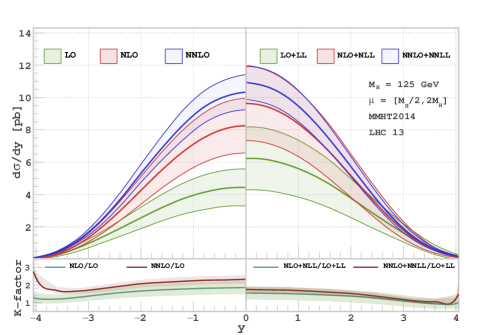
Figure 1: Higgs rapidity distributions for fixed-order (left panel) and resummed contributions (right panel) are presented with corresponding $K$ factors on lower panels around the central scale $\mu_{R}=\mu_{F}=M_{H}$.

Phenomenology.— In the following we study the numerical impact of resummed contributions up to NNLL accuracy for the rapidity distribution of a scalar Higgs boson of mass $M_{H}=125$ GeV at the LHC with $\sqrt{S}=13$ TeV. We have set the number of flavors $n_{f}=5$ and the top mass at 173 GeV and use MMHT 2014 Harland-Lang et al. (2015) PDFs along with the corresponding values of $a_{s}$ for LO, NLO, and NNLO through the LHAPDF Buckley et al. (2015) interface, unless otherwise stated. We use the publicly available code FEHIP Anastasiou et al. (2005) to obtain $d\sigma^{g,\text{f.o}}/dy$ up to NNLO level. We have developed an in-house Fortran code to perform double Mellin inversion for the resummed contributions computed in this paper. In Fig.1, using Eq.(Threshold resummation of the rapidity distribution for Higgs production at NNLO+NNLL), we present the production cross section for the scalar Higgs boson as a function of its rapidity $y$ up to NNLO in the left panel and to NNLO+NNLL in the right panel along with the respective K factors. The K factor at a given order, say, at NⁿLO (NⁿLO + NⁿLL), is defined by the cross section at that order normalized by the same at LO (LO+LL) at $\mu_{R}=\mu_{F}=M_{H}$. The symmetric band at each order is generated by varying $\mu_{R}$ and $\mu_{F}$ between $[M_{H}/2,2M_{H}]$ around the central scale $\mu_{R}=\mu_{F}=M_{H}$ with the constraint $1/2\leq\mu_{R}/\mu_{F}\leq 2$, adding and subtracting the highest possible errors from all the scale combinations to the central scale. We find that the magnitude and sign of the resummed contribution do vary depending on the order in $a_{s}$ as well the exact values of $y$ and the scales $\mu_{R},\mu_{F}$.

y	LO	LO+LL	NLO	NLO+NLL	NNLO	NNLO+NNLL	NNLO+NNNLL
0.0	$4.435\pm 1.145$	$6.231\pm 1.950$	$8.255\pm 1.684$	$9.632\pm 2.286$	$10.329\pm 1.088$	$10.938\pm 1.050$	$10.517\pm 0.820$
0.8	$4.134\pm 1.067$	$5.833\pm 1.831$	$7.517\pm 1.530$	$8.820\pm 2.124$	$9.407\pm 0.988$	$9.992\pm 1.025$	$9.641\pm 0.718$
1.6	$3.189\pm 0.819$	$4.630\pm 1.468$	$5.522\pm 1.117$	$6.611\pm 1.676$	$6.877\pm 0.744$	$7.380\pm 0.849$	$7.045\pm 0.563$
2.4	$1.904\pm 0.492$	$2.887\pm 0.942$	$2.985\pm 0.597$	$3.715\pm.998$	$3.683\pm 0.410$	$4.040\pm 0.501$	$3.821\pm 0.305$

Table 1: Fixed-order and resummed results for Higgs rapidity distribution with corresponding absolute error for different benchmark values of $y$.

In particular, at the central scale $\mu=\mu_{R}=\mu_{F}=M_{H}$, the percentage correction from the leading-logarithmic (LL) contribution goes from $40\%$ to $50\%$ whereas for next-to-leading-logarithmic (NLL), we find that it varies from $17\%$ to $24\%$ and for NNLL it varies from $6\%$ to $10\%$ in the region $0\leq y\leq 2.4$, which is evident from Table 1. Interestingly, at $\mu=M_{H}/2$, we find that the cross section at NNLO+NNLL is very close to NNLO for a wider range of $y$ indicating that $\mu=M_{H}/2$ is a good choice for the fixed-order predictions. A similar conclusion was arrived at in Ref. Anastasiou et al. (2003) for the inclusive production of the Higgs boson. From the upper-left panel of Fig.1, we also observe that LO and NLO predictions do not overlap around the central rapidity region. However, at NNLO, partial overlap indicates that the inclusion of higher-order corrections has increased the convergence of perturbation series. The upper-right panel shows the effect of resummation over the fixed-order result. We observe that LO+LL has overlap with NLO+NLL for all values of rapidity. In addition, the distribution at NNLO+NNLL falls completely within NLO+NLL band. In fact, NNLO+NNLL increases approximately by 13% with respect to NLO+NLL; the corresponding number for NNLO over NLO is approximately 25%. This implies that the perturbative convergence at the resummed level is better compared to the fixed-order result. We have also chosen $M_{H}/2$ as the central scale and found out that the choice of central scale has a minimum effect on the resummed result at NNLO+NNLL; i.e., the resum result at this order stabilizes irrespective of the above-mentioned choices, whereas at fixed order, this does not happen. Based on the above observations, we can predict that the N³LO will be very close to NNLO+NNLL and the N³LO + N³LL result will lie within the NNLO+NNLL uncertainty band. In the Table 1, the impact of N³LL on the NNLO result is also presented.

To understand the impact of unphysical scales $\mu_{R}$ and $\mu_{F}$ on our resummed results, we first varied one while fixing the other to $M_{H}$ and then varied both simultaneously for various values of rapidity $y$, the results are presented in Fig. 2. As expected, the running coupling constant decreased the cross section as we increased $\mu_{R}$, while the opposite behaviour was observed for $\mu_{F}$ both in fixed-order and in resummed results. Varying these two scales simultaneously led to a cancellation of the two different behaviors, and the amount of cancellation depended on order of perturbation $n$ and value of $y$. Finally, to study the impact of choice of PDFs, in Table 2, we have presented the results at NNLO+NNLL using the central PDF of each PDF group.

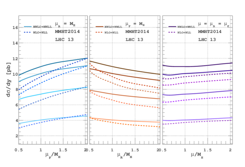
Figure 2: $\mu_{F}$, $\mu_{R}$ scale variations for the NLO+NLL (dashed) and NNLO+NNLL (solid) cases for different benchmark $y$ values (starting from the top, $y=0,0.8,1.6,2.4$).

y	MMHT	ABMP	CT10	NNPDF	PDF4LHC
0.0	$10.938$	$10.654$	$10.709$	$11.302$	$10.850$
0.8	$9.992$	$9.713$	$9.820$	$10.378$	$9.977$
1.6	$7.380$	$7.043$	$7.362$	$7.758$	$7.456$
2.4	$4.040$	$3.727$	$4.105$	$4.111$	$4.075$

Table 2: Using different PDFs, NNLO+NNLL contributions to rapidity distribution for $y=0,0.8,1.6,2.4$.

Conclusion.—In this paper, we have developed a formalism to resum threshold logarithms in double Mellin space for the rapidity distribution of a colorless final state $F$ produced in the hadron collider. We have derived for the first time compact and most general expressions for resummed exponents $g^{I}_{d}$ up to NNLO+NNLL accuracy. We find that the resummed result not only changes the fixed-order predictions but also remarkably improves the perturbative convergence. We observe that the resummed result at NNLO+NNLL stabilizes over fixed order irrespective of the choices of the central scale between $[M_{H}/2,2M_{H}]$. We have also studied the impact of PDFs on the predictions. The present study can easily be extended to Drell-Yan Banerjee et al. , pseudoscalar, and $W^{\pm}$ and $Z$ productions as well as the production of the Higgs boson in bottom-antibottom annihilation at hadron colliders.

Acknowledgements.— We are thankful for useful help from A. Vogt, F. Petriello, T. Hahn, M. Bonvini, L. Rottoli, P. Mangalapandi, T. Ahmed, N. Rana, and A. Karan. V. Ravindran would like to thank T. Gehrmann for fruitful discussions and also thanks University of Zurich, where part of the work was carried out, for hospitality.

References

- Aad et al. (2012) G. Aad et al. (ATLAS), Phys. Lett. B716, 1 (2012), arXiv:1207.7214 [hep-ex] .
- Chatrchyan et al. (2012) S. Chatrchyan et al. (CMS), Phys. Lett. B716, 30 (2012), arXiv:1207.7235 [hep-ex] .
- Anastasiou et al. (2015) C. Anastasiou, C. Duhr, F. Dulat, F. Herzog, and B. Mistlberger, Phys. Rev. Lett. 114, 212001 (2015), arXiv:1503.06056 [hep-ph] .
- Drell and Yan (1970) S. D. Drell and T.-M. Yan, Phys. Rev. Lett. 25, 316 (1970), [Erratum: Phys. Rev. Lett.25,902(1970)].
- Gao et al. (2014) J. Gao, M. Guzzi, J. Huston, H.-L. Lai, Z. Li, P. Nadolsky, J. Pumplin, D. Stump, and C. P. Yuan, Phys. Rev. D89, 033009 (2014), arXiv:1302.6246 [hep-ph] .
- Harland-Lang et al. (2015) L. A. Harland-Lang, A. D. Martin, P. Motylinski, and R. S. Thorne, Eur. Phys. J. C75, 204 (2015), arXiv:1412.3989 [hep-ph] .
- Ball et al. (2015) R. D. Ball et al. (NNPDF), JHEP 04, 040 (2015), arXiv:1410.8849 [hep-ph] .
- Butterworth et al. (2016) J. Butterworth et al., J. Phys. G43, 023001 (2016), arXiv:1510.03865 [hep-ph] .
- Alekhin et al. (2017) S. Alekhin, J. Bl mlein, S. Moch, and R. Placakyte, Phys. Rev. D96, 014011 (2017), arXiv:1701.05838 [hep-ph] .
- Khachatryan et al. (2015) V. Khachatryan et al. (CMS), Eur. Phys. J. C75, 147 (2015), arXiv:1412.1115 [hep-ex] .
- Affolder et al. (2001a) T. Affolder et al. (CDF), Phys. Rev. D63, 011101 (2001a), arXiv:hep-ex/0006025 [hep-ex] .
- Abe et al. (1998) F. Abe et al. (CDF), Phys. Rev. Lett. 81, 5754 (1998), arXiv:hep-ex/9809001 [hep-ex] .
- Affolder et al. (2001b) T. Affolder et al. (CDF), Phys. Rev. Lett. 87, 131802 (2001b), arXiv:hep-ex/0106047 [hep-ex] .
- Arkani-Hamed et al. (1998) N. Arkani-Hamed, S. Dimopoulos, and G. R. Dvali, Phys. Lett. B429, 263 (1998), arXiv:hep-ph/9803315 [hep-ph] .
- Randall and Sundrum (1999) L. Randall and R. Sundrum, Phys. Rev. Lett. 83, 3370 (1999), arXiv:hep-ph/9905221 [hep-ph] .
- Dawson (1991) S. Dawson, Nucl. Phys. B359, 283 (1991).
- Djouadi et al. (1991) A. Djouadi, M. Spira, and P. M. Zerwas, Phys. Lett. B264, 440 (1991).
- Spira et al. (1995) M. Spira, A. Djouadi, D. Graudenz, and P. M. Zerwas, Nucl. Phys. B453, 17 (1995), arXiv:hep-ph/9504378 [hep-ph] .
- Harlander and Kilgore (2001) R. V. Harlander and W. B. Kilgore, Phys. Rev. D64, 013015 (2001), arXiv:hep-ph/0102241 [hep-ph] .
- Catani et al. (2001) S. Catani, D. de Florian, and M. Grazzini, JHEP 05, 025 (2001), arXiv:hep-ph/0102227 [hep-ph] .
- Harlander and Kilgore (2002) R. V. Harlander and W. B. Kilgore, Phys. Rev. Lett. 88, 201801 (2002), arXiv:hep-ph/0201206 [hep-ph] .
- Anastasiou and Melnikov (2002) C. Anastasiou and K. Melnikov, Nucl. Phys. B646, 220 (2002), arXiv:hep-ph/0207004 [hep-ph] .
- Ravindran et al. (2003) V. Ravindran, J. Smith, and W. L. van Neerven, Nucl. Phys. B665, 325 (2003), arXiv:hep-ph/0302135 [hep-ph] .
- Kubar-Andre and Paige (1979) J. Kubar-Andre and F. E. Paige, Marseille Colloq.1978:V.85, Phys. Rev. D19, 221 (1979).
- Altarelli et al. (1978) G. Altarelli, R. K. Ellis, and G. Martinelli, Nucl. Phys. B143, 521 (1978), [Erratum: Nucl. Phys.B146,544(1978)].
- Humpert and van Neerven (1981) B. Humpert and W. L. van Neerven, Nucl. Phys. B184, 225 (1981).
- Matsuura and van Neerven (1988) T. Matsuura and W. L. van Neerven, Z. Phys. C38, 623 (1988).
- Matsuura et al. (1989) T. Matsuura, S. C. van der Marck, and W. L. van Neerven, Nucl. Phys. B319, 570 (1989).
- Hamberg et al. (1991) R. Hamberg, W. L. van Neerven, and T. Matsuura, Nucl. Phys. B359, 343 (1991), [Erratum: Nucl. Phys.B644,403(2002)].
- Anastasiou et al. (2003) C. Anastasiou, L. J. Dixon, K. Melnikov, and F. Petriello, Phys. Rev. Lett. 91, 182002 (2003), arXiv:hep-ph/0306192 [hep-ph] .
- Anastasiou et al. (2004) C. Anastasiou, K. Melnikov, and F. Petriello, Phys. Rev. Lett. 93, 262002 (2004), arXiv:hep-ph/0409088 [hep-ph] .
- Anastasiou et al. (2014) C. Anastasiou, C. Duhr, F. Dulat, E. Furlan, T. Gehrmann, F. Herzog, and B. Mistlberger, Phys. Lett. B737, 325 (2014), arXiv:1403.4616 [hep-ph] .
- Moch and Vogt (2005) S. Moch and A. Vogt, Phys. Lett. B631, 48 (2005), arXiv:hep-ph/0508265 [hep-ph] .
- Laenen and Magnea (2006) E. Laenen and L. Magnea, Phys. Lett. B632, 270 (2006), arXiv:hep-ph/0508284 [hep-ph] .
- Idilbi et al. (2006) A. Idilbi, X.-d. Ji, J.-P. Ma, and F. Yuan, Phys. Rev. D73, 077501 (2006), arXiv:hep-ph/0509294 [hep-ph] .
- Ravindran (2006a) V. Ravindran, Nucl. Phys. B746, 58 (2006a), arXiv:hep-ph/0512249 [hep-ph] .
- Ravindran (2006b) V. Ravindran, Nucl. Phys. B752, 173 (2006b), arXiv:hep-ph/0603041 [hep-ph] .
- Kumar et al. (2015) M. C. Kumar, M. K. Mandal, and V. Ravindran, JHEP 03, 037 (2015), arXiv:1412.3357 [hep-ph] .
- Ahmed et al. (2014a) T. Ahmed, N. Rana, and V. Ravindran, JHEP 10, 139 (2014a), arXiv:1408.0787 [hep-ph] .
- Ahmed et al. (2015a) T. Ahmed, G. Das, M. C. Kumar, N. Rana, and V. Ravindran, (2015a), arXiv:1505.07422 [hep-ph] .
- Ahmed et al. (2014b) T. Ahmed, M. Mahakhud, N. Rana, and V. Ravindran, Phys. Rev. Lett. 113, 112002 (2014b), arXiv:1404.0366 [hep-ph] .
- Li et al. (2014) Y. Li, A. von Manteuffel, R. M. Schabinger, and H. X. Zhu, Phys. Rev. D90, 053006 (2014), arXiv:1404.5839 [hep-ph] .
- Catani et al. (2014) S. Catani, L. Cieri, D. de Florian, G. Ferrera, and M. Grazzini, Nucl. Phys. B888, 75 (2014), arXiv:1405.4827 [hep-ph] .
- Sterman (1987) G. F. Sterman, Nucl. Phys. B281, 310 (1987).
- Catani and Trentadue (1989) S. Catani and L. Trentadue, Nucl. Phys. B327, 323 (1989).
- Catani and Trentadue (1991) S. Catani and L. Trentadue, Nucl. Phys. B353, 183 (1991).
- Bozzi et al. (2008) G. Bozzi, S. Catani, D. de Florian, and M. Grazzini, Nucl. Phys. B791, 1 (2008), arXiv:0705.3887 [hep-ph] .
- Bozzi et al. (2009) G. Bozzi, S. Catani, G. Ferrera, D. de Florian, and M. Grazzini, Nucl. Phys. B815, 174 (2009), arXiv:0812.2862 [hep-ph] .
- Bozzi et al. (2011) G. Bozzi, S. Catani, G. Ferrera, D. de Florian, and M. Grazzini, Phys. Lett. B696, 207 (2011), arXiv:1007.2351 [hep-ph] .
- Catani and Grazzini (2011) S. Catani and M. Grazzini, Nucl. Phys. B845, 297 (2011), arXiv:1011.3918 [hep-ph] .
- Catani et al. (2013) S. Catani, M. Grazzini, and A. Torre, Nucl. Phys. B874, 720 (2013), arXiv:1305.3870 [hep-ph] .
- Monni et al. (2016) P. F. Monni, E. Re, and P. Torrielli, Phys. Rev. Lett. 116, 242001 (2016), arXiv:1604.02191 [hep-ph] .
- Ebert and Tackmann (2017) M. A. Ebert and F. J. Tackmann, JHEP 02, 110 (2017), arXiv:1611.08610 [hep-ph] .
- Grazzini et al. (2015) M. Grazzini, S. Kallweit, D. Rathlev, and M. Wiesemann, JHEP 08, 154 (2015), arXiv:1507.02565 [hep-ph] .
- Ferrera and Pires (2017) G. Ferrera and J. Pires, JHEP 02, 139 (2017), arXiv:1609.01691 [hep-ph] .
- Laenen and Sterman (1992) E. Laenen and G. F. Sterman, in The Fermilab Meeting DPF 92. Proceedings, 7th Meeting of the American Physical Society, Division of Particles and Fields, Batavia, USA, November 10-14, 1992. Vol. 1, 2 (1992) pp. 987–989.
- Sterman and Vogelsang (2001) G. F. Sterman and W. Vogelsang, JHEP 02, 016 (2001), arXiv:hep-ph/0011289 [hep-ph] .
- Mukherjee and Vogelsang (2006) A. Mukherjee and W. Vogelsang, Phys. Rev. D73, 074005 (2006), arXiv:hep-ph/0601162 [hep-ph] .
- Bolzoni (2006) P. Bolzoni, Phys. Lett. B643, 325 (2006), arXiv:hep-ph/0609073 [hep-ph] .
- Becher and Neubert (2006) T. Becher and M. Neubert, Phys. Rev. Lett. 97, 082001 (2006), arXiv:hep-ph/0605050 [hep-ph] .
- Becher et al. (2008) T. Becher, M. Neubert, and G. Xu, JHEP 07, 030 (2008), arXiv:0710.0680 [hep-ph] .
- Bonvini et al. (2015) M. Bonvini, S. Forte, G. Ridolfi, and L. Rottoli, JHEP 01, 046 (2015), arXiv:1409.0864 [hep-ph] .
- Ebert et al. (2017) M. A. Ebert, J. K. L. Michel, and F. J. Tackmann, JHEP 05, 088 (2017), arXiv:1702.00794 [hep-ph] .
- Ravindran et al. (2007) V. Ravindran, J. Smith, and W. L. van Neerven, Nucl. Phys. B767, 100 (2007), arXiv:hep-ph/0608308 [hep-ph] .
- Ravindran and Smith (2007) V. Ravindran and J. Smith, Phys. Rev. D76, 114004 (2007), arXiv:0708.1689 [hep-ph] .
- Ahmed et al. (2014c) T. Ahmed, M. K. Mandal, N. Rana, and V. Ravindran, Phys. Rev. Lett. 113, 212003 (2014c), arXiv:1404.6504 [hep-ph] .
- Ahmed et al. (2015b) T. Ahmed, M. K. Mandal, N. Rana, and V. Ravindran, JHEP 02, 131 (2015b), arXiv:1411.5301 [hep-ph] .
- Ravindran et al. (2005) V. Ravindran, J. Smith, and W. L. van Neerven, Nucl. Phys. B704, 332 (2005), arXiv:hep-ph/0408315 [hep-ph] .
- Moch et al. (2005) S. Moch, J. A. M. Vermaseren, and A. Vogt, JHEP 08, 049 (2005), arXiv:hep-ph/0507039 [hep-ph] .
- Catani et al. (2003) S. Catani, D. de Florian, M. Grazzini, and P. Nason, JHEP 07, 028 (2003), arXiv:hep-ph/0306211 [hep-ph] .
- Banerjee et al. (2018) P. Banerjee, G. Das, P. K. Dhani, and V. Ravindran, Phys. Rev. D97, 054024 (2018), arXiv:1708.05706 [hep-ph] .
- Anastasiou et al. (2005) C. Anastasiou, K. Melnikov, and F. Petriello, Nucl. Phys. B724, 197 (2005), arXiv:hep-ph/0501130 [hep-ph] .
- Catani et al. (1996) S. Catani, M. L. Mangano, P. Nason, and L. Trentadue, Nucl. Phys. B478, 273 (1996), arXiv:hep-ph/9604351 [hep-ph] .
- Buckley et al. (2015) A. Buckley, J. Ferrando, S. Lloyd, K. Nordstr m, B. Page, M. R fenacht, M. Sch nherr, and G. Watt, Eur. Phys. J. C75, 132 (2015), arXiv:1412.7420 [hep-ph] .
- (75) P. Banerjee, G. Das, P. K. Dhani, and V. Ravindran, Threshold resummation of rapidity distribution for Drell-Yan production at NNLO+NNLL (in preparation).