Matrix KP: tropical limit and Yang-Baxter maps

Abstract

We study soliton solutions of matrix Kadomtsev-Petviashvili (KP) equations in a tropical limit, in which their support at fixed time is a planar graph and polarizations are attached to its constituting lines. There is a subclass of “pure line soliton solutions” for which we find that, in this limit, the distribution of polarizations is fully determined by a Yang-Baxter map. For a vector KP equation, this map is given by an $R$-matrix, whereas it is a non-linear map in case of a more general matrix KP equation. We also consider the corresponding Korteweg-deVries (KdV) reduction. Furthermore, exploiting the fine structure of soliton interactions in the tropical limit, we obtain a new solution of the tetrahedron (or Zamolodchikov) equation. Moreover, a solution of the functional tetrahedron equation arises from the parameter-dependence of the vector KP $R$-matrix.

1 Introduction

A line soliton solution of the scalar Kadomtsev-Petviashvili (KP-II) equation (see, e.g., [1]) is, at fixed time $t$, an exponentially localized wave on a plane. The “tropical limit”, in the sense of our work in [2, 3, 4] (also see [5, 6]), takes it to a piecewise linear structure, a planar graph that represents the wave crest, with values of the dependent variable attached to its edges.

In this work we consider the $m\times n$ matrix potential KP equation

$$4\phi_{xt}-\phi_{xxxx}-3\phi_{yy}-6(\phi_{x}K\phi_{x})_{x}+6(\phi_{x}K\phi_{y}-\phi_{y}K\phi_{x})=0\,,$$ (1.1)

where $K$ is a constant $n\times m$ matrix and $\phi$ an $m\times n$ matrix, depending on independent variables $x,y,t$, and a subscript indicates a corresponding partial derivative. We will refer to this equation as pKP_K.

If $\phi$ is a solution of (1.1), then $\phi_{R}:=\phi K$ and $\phi_{L}:=K\phi$ solve the ordinary $m\times m$, respectively $n\times n$, matrix potential KP equation. We also note that, if $K=TK^{\prime}S$ with a constant $m^{\prime}\times m$ matrix $S$ and a constant $n\times n^{\prime}$ matrix $T$, then the $m^{\prime}\times n^{\prime}$ matrix $\phi^{\prime}=S\phi T$ satisfies the pKP${}_{K^{\prime}}$ equation, as a consequence of (1.1).

In the vector case $n=1$, writing $K=(k_{1},\ldots,k_{m})$ and $\phi=(\phi_{1},\ldots,\phi_{m})^{\intercal}$, (1.1) becomes the following system of coupled equations,

$$4\,\phi_{i,xt}-\phi_{i,xxxx}-3\,\phi_{i,yy}-6\sum_{j=1}^{m}k_{j}\,\Big{(}(\phi_{i,x}\phi_{j,x})_{x}-\phi_{i,x}\phi_{j,y}+\phi_{i,y}\phi_{j,x}\Big{)}=0\qquad i=1,\ldots,m\,.$$

By choosing $T=1$ and any invertible $m\times m$ matrix $S$ that has $K$ as its first row, we have $K=K^{\prime}S$ with $K^{\prime}=(1,0,\ldots,0)$. In terms of the new variable $\phi^{\prime}=S\phi$, the above system thus consists of one scalar pKP equation and $m-1$ linear equations involving the dependent variable of the former.

For

$$u:=2\,\phi_{x}\,,$$

we obtain from (1.1) the $m\times n$ matrix KP equation

$$(\,4\,u_{t}-u_{xxx}-3\,(uKu)_{x}\,)_{x}-3\,u_{yy}+3\,\Big{(}uK\int u_{y}\,dx-\int u_{y}\,dx\,Ku\Big{)}_{x}=0\,.$$ (1.2)

The extension of the scalar KP equation to a matrix version achieves that solitons carry internal degrees of freedom, “polarization”.

The Korteweg-deVries (KdV) reduction of (1.2) is

$$4\,u_{t}-u_{xxx}-3\,(uKu)_{x}=0\,,$$ (1.3)

which we will refer to as KdV_K. If $K$ is the identity matrix, this is the matrix KdV equation (see, e.g., [7]). The 2-soliton solution of the latter yields a map from polarizations at $t\ll 0$ to polarizations at $t\gg 0$. It is known [8, 9] that this yields a Yang-Baxter map, i.e., a set-theoretical solution of the (quantum) Yang-Baxter equation (also see [10] for the case of the vector Nonlinear Schrödinger equation). Not surprisingly, this is a feature preserved in the tropical limit. The surprising new insight, however, is that this map governs the evolution of polarizations throughout the tropical limit graph of a soliton solution. In case of a vector KdV equation, i.e., KdV_K with $n=1$, it is given by an $R$-matrix, a linear map solution of the Yang-Baxter equation.

More generally, we will explore in this work the tropical limit of “pure” (see Section 3) soliton solutions of the above $K$-modified matrix KP equation and demonstrate that a Yang-Baxter map governs their structure.

In case of the vector KP equation, the expression for a pure soliton solution involves a function $\tau$ which is a $\tau$-function of the scalar KP equation. Its tropical limit at fixed $t$ determines a planar graph, and the vector KP soliton solution associates in this limit a constant vector (polarization) with each linear segment of the graph. The polarization values are then related by a linear Yang-Baxter map, represented by an $R$-matrix, which does not depend on the independent variables $x,y,t$, but only on the “spectral parameters” of the soliton solution.

Section 2 summarizes a binary Darboux transformation for the pKP_K equation and applies it to a trivial seed solution in order to obtain soliton solutions. In Section 3 we restrict out consideration to the subclass of “pure” soliton solutions. This essentially disregards solutions with substructures of the form of Miles resonances. Section 4 addresses the tropical limit of pure soliton solutions. The cases of two and three solitons are then treated in Sections 5 and 6. Section 7 provides a general proof of the fact that, in the vector case, an $R$-matrix relates the polarizations at crossings. The linearity of the Yang-Baxter map in the vector case is certainly related to the particularly simple structure of the vector pKP equation mentioned above. In Section 8 we show how to construct a pure $N$-soliton solution of the vector KP equation from a pure $N$-soliton solution of the scalar KP equation, $N$ vector data and the aforementioned $R$-matrix. Section 9 extends our exploration of the vector KP 3-soliton case and presents an apparently new solution of the tetrahedron (Zamolodchikov) equation (see, e.g., [11] and references cited there). In Section 10 we reveal the structure of the vector KP $R$-matrix, which leads us to a more general two-parameter $R$-matrix. Its parameter-dependence determines, via a “local” Yang-Baxter equation [12] (also see [11]), a solution of the functional tetrahedron equation (see, e.g., [13, 14, 11]), i.e., the set-theoretical version of the tetrahedron equation. Finally, Section 11 contains some concluding remarks.

2 Soliton solutions of the $K$-modified matrix KP equation

The following describes a binary Darboux transformation for the pKP_K equation (1.1). This is a simple extension of what is presented in [15], for example. Let $\phi_{0}$ be a solution of (1.1). Let $\theta$ and $\chi$ be $m\times N$, respectively $N\times n$, matrix solutions of the linear equations

$$\theta_{y}=\theta_{xx}+2\phi_{0,x}K\theta\,,\qquad\theta_{t}=\theta_{xxx}+3\phi_{0,x}K\theta_{x}+\frac{3}{2}(\phi_{0,y}+\phi_{0,xx})K\theta\,,$$

$$\chi_{y}=-\chi_{xx}-2\chi K\phi_{0,x}\,,\qquad\chi_{t}=\chi_{xxx}+3\chi_{x}K\phi_{0,x}-\frac{3}{2}\chi K(\phi_{0,y}-\phi_{0,xx})\,.$$

Then the system

$$\Omega_{x}=-\chi K\theta\,,\quad\Omega_{y}=-\chi K\theta_{x}+\chi_{x}K\theta\,,\quad\Omega_{t}=-\chi K\theta_{xx}+\chi_{x}K\theta_{x}-\chi_{xx}K\theta-3\chi K\phi_{0,x}K\theta\,,$$ (2.1)

is compatible and can thus be integrated to yield an $N\times N$ matrix solution $\Omega$. If $\Omega$ is invertible, then

$$\phi=\phi_{0}-\theta\,\Omega^{-1}\chi$$ (2.2)

is a new solution of (1.1).

For vanishing seed solution, i.e., $\phi_{0}=0$, soliton solutions are obtained as follows. Let

$$\theta=\sum_{a=1}^{A}\theta_{a}\,e^{\vartheta(P_{a})}\,,\qquad\chi=\sum_{b=1}^{B}e^{-\vartheta(Q_{b})}\,\chi_{b}\,,$$

where $P_{a},Q_{b}$ are constant $N\times N$ matrices, $\theta_{a},\chi_{b}$ are constant $m\times N$, respectively $N\times n$ matrices, and

$$\vartheta(P)=x\,P+y\,P^{2}+t\,P^{3}\,.$$ (2.3)

If, for all $a,b$, the matrices $P_{a}$ and $Q_{b}$ have no eigenvalue in common, there are unique $N\times N$ matrix solutions $W_{ba}$ of the Sylvester equations

$$Q_{b}W_{ba}-W_{ba}P_{a}=\chi_{b}K\theta_{a}\qquad a=1,\ldots,A,\quad b=1,\ldots,B\,.$$

Then (2.1) is solved by

$$\Omega=\Omega_{0}+\sum_{a=1}^{A}\sum_{b=1}^{B}e^{-\vartheta(Q_{b})}\,W_{ba}\,e^{\vartheta(P_{a})}\,,$$

with a constant $N\times N$ matrix $\Omega_{0}$, and (2.2) determines a soliton solution of (1.1) (and thus via $u=2\,\phi_{x}$ a solution of (1.2)), if $\Omega$ is everywhere invertible.

Remark 2.1.

Corresponding solutions of the pKP_K hierarchy are obtained by replacing (2.3) with $\vartheta(P)=\sum_{r=1}^{\infty}t_{r}\,P^{r}$, where $t_{1}=x$, $t_{2}=y$, $t_{3}=t$. $\square$

3 Pure soliton solutions

In the following we restrict our considerations to the case where $A=B=1$. Then there remains only a single Sylvester equation,

$$Q_{1}W-WP_{1}=\chi_{1}K\theta_{1}\,.$$

Moreover, we will restrict the matrices $P_{1}$ and $Q_{1}$ to be diagonal. It is convenient to name the diagonal entries (“spectral parameters”) in two different ways,

$$P_{1}=\mathrm{diag}(p_{1,1},\ldots,p_{N,1})=\mathrm{diag}(p_{1},\ldots,p_{N})\,,$$

$$Q_{1}=\mathrm{diag}(p_{1,2},\ldots,p_{N,2})=\mathrm{diag}(q_{1},\ldots,q_{N})\,.$$

We further write

$$\theta_{1}=\left(\begin{array}[]{cccc}(q_{1}-p_{1})\xi_{1}&(q_{2}-p_{2})\xi_{2}&\cdots&(q_{N}-p_{N})\xi_{N}\end{array}\right)\,,\qquad\chi_{1}=\left(\begin{array}[]{c}\eta_{1}\\ \vdots\\ \eta_{N}\end{array}\right)\,,$$

where $\xi_{i}$ are $m$-component column vectors and $\eta_{i}$ are $n$-component row vectors. Then the solution of the above Sylvester equation is given by

$$W=(w_{ij})\,,\qquad w_{ij}=\frac{q_{j}-p_{j}}{q_{i}-p_{j}}\,\eta_{i}\,K\,\xi_{j}\qquad i,j=1,\ldots,N\,.$$

Furthermore, we set $\Omega_{0}=I_{N}$, the $N\times N$ identity matrix. Hence $\Omega=(\Omega_{ij})$ with

$$\Omega_{ij}=\delta_{ij}+w_{ij}\,e^{\vartheta(p_{j})-\vartheta(q_{i})}\,,$$ (3.2)

where $\delta_{ij}$ is the Kronecker delta. We call soliton solutions obtained from (2.2), with the above restrictions, “pure solitons”. All what follows refers to them.

We introduce

$$\vartheta_{I}:=\sum_{i=1}^{N}\vartheta(p_{i,a_{i}})\qquad\mbox{if}\quad I=(a_{1},\ldots,a_{N})\in\{1,2\}^{N}\,.$$

Instead of using $(a_{1},\ldots,a_{N})$ as a subscript (or superscript), we will simply write $a_{1}\ldots a_{N}$ in the following. For example, $\vartheta_{a_{1}\ldots a_{N}}=\vartheta_{(a_{1},\ldots,a_{N})}$.

From (2.2) we find that the pure soliton solutions of the pKP_K equation are given by

$$\phi=\frac{F}{\tau}\,,$$ (3.3)

with

$$\tau := e^{\vartheta_{\boldsymbol{2}}}\,\det\Omega\,,$$ (3.4)

$$F := -e^{\vartheta_{\boldsymbol{2}}}\,\theta_{1}\,e^{\vartheta(P_{1})}\,\mathrm{adj}(\Omega)\,e^{-\vartheta(Q_{1})}\,\chi_{1}\,,$$ (3.5)

where $\mathrm{adj}(\Omega)$ denotes the adjugate of the matrix $\Omega$ and $\boldsymbol{2}:=2\ldots 2=(2,\ldots,2)$.

Proposition 3.1.

$\tau$ and $F$ have expansions

$$\tau=\sum_{I\in\{1,2\}^{N}}\mu_{I}\,e^{\vartheta_{I}}\,,$$ (3.6)

$$F=\sum_{I\in\{1,2\}^{N}}M_{I}\,e^{\vartheta_{I}}\,,$$ (3.7)

with constants $\mu_{I}$ and constant $m\times n$ matrices $M_{I}$, where $\mu_{\boldsymbol{2}}=1$ and $M_{\boldsymbol{2}}=0$.

Proof.

From the definition of the determinant, $\det\Omega=\epsilon^{i_{1}\ldots i_{N}}\,\Omega_{1i_{1}}\cdots\Omega_{Ni_{N}}$, with the Levi-Civita symbol $\epsilon^{i_{1}\ldots i_{N}}$ and summation convention, we know that $\det\Omega$ consists of a sum of monomials of order $N$ in the entries $\Omega_{ij}$. Here the latter are given by (3.2). If no diagonal term $\Omega_{ii}$ appears in a monomial, its phase factor is $e^{\vartheta_{\boldsymbol{1}}-\vartheta_{\boldsymbol{2}}}$. If one diagonal entry $\Omega_{ii}=1+w_{ii}\,e^{\vartheta(p_{i,1})-\vartheta(p_{i,2})}$ appears in a monomial, the latter splits into two parts. Only the part arising from the summand $1$ is different as now the phase factor is $e^{\vartheta_{\boldsymbol{1}}-\vartheta_{\boldsymbol{2}}-\vartheta(p_{i,1})+\vartheta(p_{i,2})}$. From monomials containing several diagonal entries of $\Omega$, we obtain summands with a phase factor of the form

$$e^{\vartheta_{\boldsymbol{1}}-\vartheta_{\boldsymbol{2}}-\vartheta(p_{i_{1},1})+\vartheta(p_{i_{1},2})+\cdots-\vartheta(p_{i_{r},1})+\vartheta(p_{i_{r},2})}=e^{[\vartheta_{\boldsymbol{1}}-\vartheta(p_{i_{1},1})-\cdots-\vartheta(p_{i_{r},1})]+\vartheta(p_{i_{1},2})+\cdots+\vartheta(p_{i_{r},2})-\vartheta_{\boldsymbol{2}}}\,.$$

Finally, from a monomial with $N$ diagonal entries of $\Omega$, we also obtain a constant term, namely $1$. Now our assertion (3.6) follows since $\tau$ is $\det\Omega$ multiplied by $e^{\vartheta_{\boldsymbol{2}}}$. Clearly, $\mu_{\boldsymbol{2}}=1$.

According to the Laplace (cofactor) expansion $\det\Omega=\sum_{j=1}^{N}\Omega_{ij}\,\mathrm{adj}(\Omega)_{ji}$ with respect to the $i$-th row, the term $\Omega_{ij}\,\mathrm{adj}(\Omega)_{ji}$ consists of all summands in $\det\Omega$ having $\Omega_{ij}$ as a factor. (3.6) implies that a summand of $e^{\vartheta_{\boldsymbol{2}}}\mathrm{adj}(\Omega)_{ji}$ then has a phase factor of the form $e^{\vartheta_{I}-\vartheta(p_{j,1})+\vartheta(p_{i,2})}$, with some $I\in\{1,2\}^{N}$, so that $e^{\vartheta_{\boldsymbol{2}}}\,(e^{\vartheta(P_{1})}\,\mathrm{adj}(\Omega)\,e^{-\vartheta(Q_{1})})_{ji}$ has the phase factor $e^{\vartheta_{I}}$. Hence (3.7) holds. Furthermore, no entry of $e^{\vartheta(P_{1})}\,\mathrm{adj}(\Omega)\,e^{-\vartheta(Q_{1})}$ is constant, hence $M_{\boldsymbol{2}}=0$. ∎

Remark 3.2.

The introduction of the redundant factor $e^{\vartheta_{\boldsymbol{2}}}$ in (3.3), via the definitions (3.4) and (3.5), achieves that $\tau$ and $F$ are linear combinations of exponentials $e^{\vartheta_{I}}$, $I\in\{1,2\}^{N}$, in which case we have a very convenient labelling. This is also so if we choose the factor $e^{-\vartheta_{\boldsymbol{1}}}$ instead, which leads to an expansion in terms of $e^{-\vartheta_{I}}$, now with $M_{\boldsymbol{1}}=0$. $\square$

Regularity of a pure soliton solution requires $\mu_{I}\geq 0$ for all $I\in\{1,2\}^{N}$ (or equivalently $\mu_{I}\leq 0$ for all $I\in\{1,2\}^{N}$) and $\mu_{I}\neq 0$ for at least one $I$. If $\mu_{I}=0$ for some $I$, this means that the phase $\vartheta_{I}$ is not present in the expression for $\tau$. In this case one has to arrange the data in such a way that $M_{I}=0$ in order to avoid unbounded exponential growth of the soliton solution in some phase region. But we will disregard such cases and add the condition $\mu_{I}>0$, $\forall I\in\{1,2\}^{N}$, to our definition of pure soliton solutions.

It follows that the corresponding solution of the KP equation is given by

$$u=\frac{1}{\tau^{2}}\sum_{I,J\in\{1,2\}^{N}}(p_{J}-p_{I})(\mu_{I}M_{J}-\mu_{J}M_{I})\,e^{\vartheta_{I}}\,e^{\vartheta_{J}}\,,$$

where

$$p_{I}=p_{1,a_{1}}+\cdots+p_{N,a_{N}}\quad\mbox{if}\quad I=(a_{1},\ldots,a_{N})\,.$$

Using Jacobi’s formula for the derivative of a determinant, we obtain

$$\tau_{x} = p_{\boldsymbol{2}}\,\tau+e^{\vartheta_{\boldsymbol{2}}}\,\mathrm{tr}(\mathrm{adj}(\Omega)\,\Omega_{x})=p_{\boldsymbol{2}}\,\tau-e^{\vartheta_{\boldsymbol{2}}}\,\mathrm{tr}(\mathrm{adj}(\Omega)\,\chi K\theta)=p_{\boldsymbol{2}}\,\tau-e^{\vartheta_{\boldsymbol{2}}}\,\mathrm{tr}(K\theta\,\mathrm{adj}(\Omega)\,\chi)$$

$$= p_{\boldsymbol{2}}\,\tau+\mathrm{tr}(K\,F)\,,$$

which implies

$$\mathrm{tr}(K\phi)=(\ln\tau)_{x}-p_{\boldsymbol{2}}\,,$$ (3.8)

and thus

$$\mathrm{tr}(Ku)=2\,(\ln\tau)_{xx}\,.$$

Using (3.3) in (3.8), and reading off the coefficient of $e^{\vartheta_{I}}$, we find

$$\mathrm{tr}(K\,M_{I})=(p_{I}-p_{\boldsymbol{2}})\,\mu_{I}\,.$$ (3.9)

Remark 3.3.

If $n=1$, (3.8) reads

$$K\phi=(\ln\tau)_{x}-p_{\boldsymbol{2}}\,,$$

and

$$Ku=2\,(\ln\tau)_{xx}$$

is a solution of the scalar KP equation. If $n>1$, $\mathrm{tr}(Ku)$ is not in general a solution of the scalar KP equation. $\square$

Remark 3.4.

Dropping the redundant factor $e^{\vartheta_{\boldsymbol{2}}}$ in (3.4) and (3.5) means that we have to multiply the above expressions (3.6) and (3.7) for $\tau$ and $F$ by $e^{-\vartheta_{\boldsymbol{2}}}$. It is then evident that $\phi$ only depends on differences of phases of the form $\vartheta(p_{i,1})-\vartheta(p_{i,2})=(p_{i,1}-p_{i,2})\,x+(p_{i,1}^{2}-p_{i,2}^{2})\,y+(p_{i,1}^{3}-p_{i,2}^{3})\,t$. As a consequence, setting $p_{i,2}=-p_{i,1}$, i.e., $q_{i}=-p_{i}$, eliminates the $y$-terms in all phases. This means that, under this condition for the parameters, we could have started as well with $\vartheta(P)=x\,P+t\,P^{3}$, hence without the $y$-term in (2.3). In this way we make contact with the KdV_K reduction of KP_K. $\square$

4 Tropical limit of pure soliton solutions

A crucial point is that we define the tropical limit of the matrix soliton solution via the tropical limit of the scalar function $\tau$ (cf. [2, 3, 4]). Let

$$\phi_{I}:=\phi\Big{|}_{\vartheta_{J}\to-\infty,J\neq I}=\frac{M_{I}}{\mu_{I}}\,.$$ (4.1)

In a region where a phase $\vartheta_{I}$ dominates all others, in the sense that $\log(\mu_{I}\,e^{\vartheta_{I}})>\log(\mu_{J}\,e^{\vartheta_{J}})$ for all participating $J\neq I$, the tropical limit of the potential $\phi$ is given by (4.1). It should be noticed that these expressions do not depend on the coordinates $x,y,t$.

The boundary between the regions associated with the phases $\vartheta_{I}$ and $\vartheta_{J}$ is determined by the condition

$$\mu_{I}\,e^{\vartheta_{I}}=\mu_{J}\,e^{\vartheta_{J}}\,.$$ (4.2)

Not all parts of such a boundary are visible at fixed time, since some of them may lie in a region where a third phase dominates the two phases. The tropical limit of a soliton solution at a fixed time $t$ has support on the visible parts of the boundaries between the regions associated with phases appearing in $\tau$. On such a visible boundary segment, the value of $u$ is given by

$$u_{IJ}=\frac{1}{2}(p_{I}-p_{J})\left(\phi_{I}-\phi_{J}\right)\,.$$

For $I=(a_{1},\ldots,a_{N})$ we set

$$I_{k}(a)=(a_{1},\ldots,a_{k-1},a,a_{k+1},\ldots,a_{N})\,.$$

At fixed time, the set of line segments associated with the $k$-th soliton are obtained from (4.2) with $I=I_{k}(1)$ and $J=I_{k}(2)$, for all possible $I$. They satisfy

$$(p_{k,2}-p_{k,1})\,x+(p_{k,2}^{2}-p_{k,1}^{2})\,y+(p_{k,2}^{3}-p_{k,1}^{3})\,t+\ln\frac{\mu_{I_{k}(2)}}{\mu_{I_{k}(1)}}=0\,.$$ (4.3)

All these line segments have the same slope $-(p_{k,2}+p_{k,1})^{-1}$ in the $xy$-plane, hence they are parallel. The shifts between them are given by

$$\delta^{(k)}_{IJ}=\ln\Big{(}\frac{\mu_{I_{k}(2)}}{\mu_{I_{k}(1)}}\frac{\mu_{J_{k}(1)}}{\mu_{J_{k}(2)}}\Big{)}\,.$$

They give rise to the familiar asymptotic “phase shifts” of line solitons. The tropical limit of $u$ on a visible line segment of the $k$-th soliton is given by

$$u_{I_{k}(1)\,I_{k}(2)}=\frac{1}{2}(p_{k,1}-p_{k,2})\left(\phi_{I_{k}(1)}-\phi_{I_{k}(2)}\right)\,.$$

The value of $u$ at a visible triple phase coincidence is

$$u_{IJL}=\frac{4}{9}(u_{IJ}+u_{IL}+u_{JL})\ =\frac{2}{9}\Big{(}(2p_{I}-p_{J}-p_{L})\phi_{I}+(2p_{J}-p_{I}-p_{L})\phi_{J}+(2p_{L}-p_{I}-p_{J})\phi_{L}\Big{)}\,.$$

Instead of the above expressions for the tropical values of $u$ we will rather consider

$$\hat{u}_{IJ}=\frac{\phi_{I}-\phi_{J}}{p_{I}-p_{J}}\,,$$ (4.4)

which has the form of a discrete derivative. Since (3.9) and (4.1) imply

$$\mathrm{tr}(K\phi_{I})=p_{I}-p_{\boldsymbol{2}}\,,$$ (4.5)

the latter values are normalized in the sense that

$$\mathrm{tr}(K\hat{u}_{IJ})=1\,.$$ (4.6)

If $I=(a_{1},\ldots,a_{N})$ and $i\neq j$, let

$$I_{ij}(a,b)=(a_{1},\ldots,a_{N})\Big{|}_{a_{i}\mapsto a,a_{j}\mapsto b}\,.$$

The normalized tropical values of $u$ satisfy

$$(p_{i}-q_{i})\,\hat{u}_{I_{ij}(1,1)\,I_{ij}(2,1)}+(p_{j}-q_{j})\,\hat{u}_{I_{ij}(2,1)\,I_{ij}(2,2)}=(p_{i}-q_{i}+p_{j}-q_{j})\,\hat{u}_{I_{ij}(1,1)\,I_{ij}(2,2)}\,,$$

$$(p_{i}-q_{i})\,\hat{u}_{I_{ij}(1,2)\,I_{ij}(2,2)}+(p_{j}-q_{j})\,\hat{u}_{I_{ij}(1,1)\,I_{ij}(1,2)}=(p_{i}-q_{i}+p_{j}-q_{j})\,\hat{u}_{I_{ij}(1,1)\,I_{ij}(2,2)}\,,$$

$$(p_{i}-q_{i})\,\hat{u}_{I_{ij}(1,1)\,I_{ij}(2,1)}+(p_{j}-q_{j})\,\hat{u}_{I_{ij}(1,1),I_{ij}(1,2)}=(p_{i}-q_{i}+q_{j}-p_{j})\,\hat{u}_{I_{ij}(1,2)\,I_{ij}(2,1)}\,,$$

$$(p_{i}-q_{i})\,\hat{u}_{I_{ij}(1,2)\,I_{ij}(2,2)}+(p_{j}-q_{j})\,\hat{u}_{I_{ij}(2,1),I_{ij}(2,2)}=(p_{i}-q_{i}+q_{j}-p_{j})\,\hat{u}_{I_{ij}(1,2)\,I_{ij}(2,1)}\,.$$

These identities are simply consequences of the definition of $\hat{u}_{IJ}$. They linearly relate the (normalized) polarizations at points of the tropical limit graph, where three lines meet.

5 Pure 2-soliton solutions

Let $N=2$. Then we have

$$\tau=e^{\vartheta_{22}}+\kappa_{11}\,e^{\vartheta_{12}}+\kappa_{22}\,e^{\vartheta_{21}}+\alpha\,\kappa_{11}\kappa_{22}\,e^{\vartheta_{11}}\,,$$

where

$$\kappa_{ij}=\eta_{i}K\xi_{j}\,,\qquad\alpha=1-\frac{(q_{1}-p_{1})(q_{2}-p_{2})\,\kappa_{12}\,\kappa_{21}}{(q_{1}-p_{2})(q_{2}-p_{1})\,\kappa_{11}\,\kappa_{22}}\,,$$

and

$$F = (q_{1}-p_{1})(q_{2}-p_{2})\,\Big{(}\frac{\kappa_{22}}{p_{2}-q_{2}}\,\xi_{1}\otimes\eta_{1}+\frac{\kappa_{11}}{p_{1}-q_{1}}\,\xi_{2}\otimes\eta_{2}+\frac{\kappa_{12}}{q_{1}-p_{2}}\,\xi_{1}\otimes\eta_{2}$$

$$+\frac{\kappa_{21}}{q_{2}-p_{1}}\,\xi_{2}\otimes\eta_{1}\Big{)}e^{\vartheta_{11}}+(p_{1}-q_{1})\,\xi_{1}\otimes\eta_{1}\,e^{\vartheta_{12}}+(p_{2}-q_{2})\,\xi_{2}\otimes\eta_{2}\,e^{\vartheta_{21}}\,.$$

The tropical values of the pKP_K solution $\phi$ in the dominant phase regions are then given by

$$\phi_{11}=\frac{(q_{1}-p_{1})(q_{2}-p_{2})}{\alpha\,\kappa_{11}\,\kappa_{22}}\Big{(}\frac{\kappa_{22}}{p_{2}-q_{2}}\,\xi_{1}\otimes\eta_{1}+\frac{\kappa_{11}}{p_{1}-q_{1}}\,\xi_{2}\otimes\eta_{2}$$

$$\hskip 42.67912pt+\frac{\kappa_{12}}{q_{1}-p_{2}}\,\xi_{1}\otimes\eta_{2}+\frac{\kappa_{21}}{q_{2}-p_{1}}\,\xi_{2}\otimes\eta_{1}\Big{)}\,,$$

$$\phi_{12}=(p_{1}-q_{1})\frac{\xi_{1}\otimes\eta_{1}}{\kappa_{11}}\,,\quad\phi_{21}=(p_{2}-q_{2})\frac{\xi_{2}\otimes\eta_{2}}{\kappa_{22}}\,,\quad\phi_{22}=0\,.$$

Remark 5.1.

The above values $\phi_{ab}$ solve the following nonlinear equation,

$$\Big{(}1+\mathrm{tr}\frac{K(\phi_{12}-\phi_{22})K(\phi_{21}-\phi_{22})}{(q_{1}-p_{2})(p_{1}-q_{2})}\Big{)}(\phi_{11}-\phi_{22})-\frac{(\phi_{12}-\phi_{22})K(\phi_{21}-\phi_{22})}{q_{1}-p_{2}}$$

$$+\frac{(\phi_{21}-\phi_{22})K(\phi_{12}-\phi_{22})}{p_{1}-q_{2}}-(\phi_{12}-\phi_{22})-(\phi_{21}-\phi_{22})=0\,.$$ (5.1)

Addressing more than two solitons, non-zero counterparts of $\phi_{22}$ will show up, as displayed in this equation. $\square$

For the tropical values of $\hat{u}$ along the phase region boundaries, we obtain

$$u_{1,\mathrm{in}}:=\hat{u}_{11,21}=\alpha^{-1}\Big{(}1_{m}-\frac{q_{2}-p_{2}}{q_{2}-p_{1}}\,\frac{\xi_{2}\otimes\eta_{2}}{\kappa_{22}}K\Big{)}\frac{\xi_{1}\otimes\eta_{1}}{\kappa_{11}}\Big{(}1_{n}-\frac{q_{2}-p_{2}}{q_{1}-p_{2}}K\frac{\xi_{2}\otimes\eta_{2}}{\kappa_{22}}\Big{)}\,,$$

$$u_{2,\mathrm{in}}:=\hat{u}_{21,22}=\frac{\xi_{2}\otimes\eta_{2}}{\kappa_{22}}\,,$$

$$u_{1,\mathrm{out}}:=\hat{u}_{12,22}=\frac{\xi_{1}\otimes\eta_{1}}{\kappa_{11}}\,,$$

$$u_{2,\mathrm{out}}:=\hat{u}_{11,12}=\alpha^{-1}\Big{(}1_{m}-\frac{q_{1}-p_{1}}{q_{1}-p_{2}}\,\frac{\xi_{1}\otimes\eta_{1}}{\kappa_{11}}K\Big{)}\frac{\xi_{2}\otimes\eta_{2}}{\kappa_{22}}\Big{(}1_{n}-\frac{q_{1}-p_{1}}{q_{2}-p_{1}}K\frac{\xi_{1}\otimes\eta_{1}}{\kappa_{11}}\Big{)}\,,$$ (5.2)

where $1_{m}$ stands for the $m\times m$ identity matrix. For the in/out classification, see Fig. 1 below. All the matrices in (5.2) have rank one, which is not at all obvious from the form of $\phi_{ab}$. We obtain the following nonlinear relation between “incoming” and “outgoing” polarizations,

$$u_{1,\mathrm{out}}=\alpha_{\mathrm{in}}^{-1}\Big{(}1_{m}-\frac{q_{2}-p_{2}}{p_{1}-p_{2}}u_{2,\mathrm{in}}K\Big{)}u_{1,\mathrm{in}}\Big{(}1_{n}-\frac{p_{2}-q_{2}}{q_{1}-q_{2}}Ku_{2,\mathrm{in}}\Big{)}\,,$$

$$u_{2,\mathrm{out}}=\alpha_{\mathrm{in}}^{-1}\Big{(}1_{m}-\frac{q_{1}-p_{1}}{q_{1}-q_{2}}u_{1,\mathrm{in}}K\Big{)}u_{2,\mathrm{in}}\Big{(}1_{n}-\frac{p_{1}-q_{1}}{p_{1}-p_{2}}Ku_{1,\mathrm{in}}\Big{)}\,,$$ (5.3)

where

$$\alpha_{\mathrm{in}}=1-\frac{(p_{1}-q_{1})(p_{2}-q_{2})}{(p_{1}-p_{2})(q_{1}-q_{2})}\mathrm{tr}\left(Ku_{1,\mathrm{in}}Ku_{2,\mathrm{in}}\right)\,.$$

We note that $\alpha\,\alpha_{\mathrm{in}}=1$. (5.3) is a new nonlinear Yang-Baxter map with parameters $p_{i},q_{i}$, $i=1,2$.

Writing

$$u_{a,\mathrm{in}}=\frac{\xi_{a,\mathrm{in}}\otimes\eta_{a,\mathrm{in}}}{\eta_{a,\mathrm{in}}K\xi_{a,\mathrm{in}}}\,,\quad u_{a,\mathrm{out}}=\frac{\xi_{a,\mathrm{out}}\otimes\eta_{a,\mathrm{out}}}{\eta_{a,\mathrm{out}}K\xi_{a,\mathrm{out}}}\qquad a=1,2\,,$$

determines $\xi_{1,\mathrm{in/out}}$ and $\eta_{1,\mathrm{in/out}}$ up to scalings. We find

$$\xi_{1,\mathrm{out}}=\alpha_{\mathrm{in}}^{-1/2}\Big{(}1_{m}-\frac{p_{2}-q_{2}}{p_{2}-p_{1}}\,\frac{\xi_{2,\mathrm{in}}\otimes\eta_{2,\mathrm{in}}}{\eta_{2,\mathrm{in}}K\xi_{2,\mathrm{in}}}K\Big{)}\xi_{1,\mathrm{in}}\,,$$

$$\xi_{2,\mathrm{out}}=\alpha_{\mathrm{in}}^{-1/2}\Big{(}1_{m}-\frac{q_{1}-p_{1}}{q_{1}-q_{2}}\,\frac{\xi_{1,\mathrm{in}}\otimes\eta_{1,\mathrm{in}}}{\eta_{1,\mathrm{in}}K\xi_{1,\mathrm{in}}}K\Big{)}\xi_{2,\mathrm{in}}\,,$$

$$\eta_{1,\mathrm{out}}=\alpha_{\mathrm{in}}^{-1/2}\eta_{1,\mathrm{in}}\Big{(}1_{n}-\frac{q_{2}-p_{2}}{q_{2}-q_{1}}\,K\,\frac{\xi_{2,\mathrm{in}}\otimes\eta_{2,\mathrm{in}}}{\eta_{2,\mathrm{in}}K\xi_{2,\mathrm{in}}}\Big{)}\,,$$

$$\eta_{2,\mathrm{out}}=\alpha_{\mathrm{in}}^{-1/2}\eta_{2,\mathrm{in}}\Big{(}1_{n}-\frac{p_{1}-q_{1}}{p_{1}-p_{2}}\,K\,\frac{\xi_{1,\mathrm{in}}\otimes\eta_{1,\mathrm{in}}}{\eta_{1,\mathrm{in}}K\xi_{1,\mathrm{in}}}\Big{)}\,,$$

and

$$(\xi_{1,\mathrm{in}},\eta_{1,\mathrm{in}};\xi_{2,\mathrm{in}},\eta_{2,\mathrm{in}})\mapsto(\xi_{1,\mathrm{out}},\eta_{1,\mathrm{out}};\xi_{2,\mathrm{out}},\eta_{2,\mathrm{out}})$$

is another form of the above Yang-Baxter map.

Remark 5.2.

In (5.2) we found that $u_{2,in}$ and $u_{1,out}$ have a simple elementary form. They are the polarizations at the two boundary lines of the dominating phase region numbered by $22=(2,2)$, see Fig. 1. We know from Proposition 3.1 that it is special since $M_{22}=0$. Considering an “evolution” in negative $x$-direction (instead of $y$-direction), thus offers a more direct derivation of the Yang-Baxter map. $\square$

Example 5.3.

Let $m=3$ and $n=2$. Choosing

$$p_{1}=-3/4\,,\quad p_{2}=1/4\,,\quad q_{1}=-1/4\,,\quad q_{2}=3/4\,,$$

and

$$\eta_{1}=(1,0)\,,\quad\eta_{2}=(0,1)\,,\quad\xi_{1}=\left(\begin{array}[]{c}2/3\\ 5\\ -2\end{array}\right)\,,\quad\xi_{2}=\left(\begin{array}[]{c}1\\ 2/3\\ 2\end{array}\right)\,,\quad K=\left(\begin{array}[]{ccc}1&1&1\\ 1&2&1\end{array}\right)\,,$$

we obtain the first contour plot, at $t=0$, shown in Fig. 1. Fig. 2 shows plots of the components of the transpose of $u$. Choosing instead $p_{2}$ close to $q_{1}$ reveals an “inner structure” of crossing points, see the second plot in Fig. 1. This is the (phase) shift mentioned in Section 4.

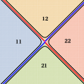
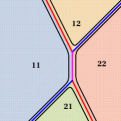
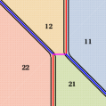
Figure 1: The first is a contour plot of $\mathrm{tr}(Ku)=2(\ln\tau)_{xx}$ for a 2-soliton solution of the $2\times 3$ matrix KP equation, at $t=0$ in the $xy$-plane, using the data of Example 5.3. Viewed as a process in $y$-direction, the YB map takes the values of the KP variable on the lower two legs to those on the upper two. A number $ij$ indicates the respective dominating phase region. In the second plot the value of $p_{2}$ is replaced by $-1/4+10^{-5}$, so that $p_{2}$ is very close to $q_{1}$. Here a boundary segment between phase regions $11$ and $22$ is visible. The third plot presents an example, where the parameters of the 2-soliton solution are now chosen such that the latter boundary is hidden and instead a boundary segment between phase regions $12$ and $21$ is visible.

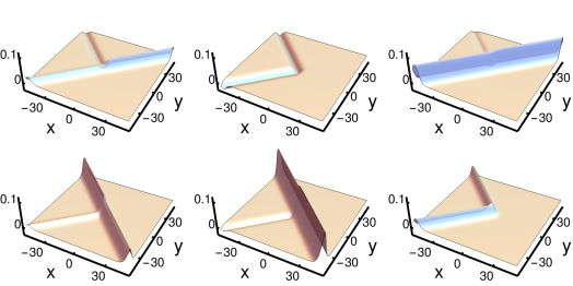
Figure 2: Plot of the six components of the transpose of $u$ at $t=0$ for the solution of the $3\times 2$ matrix KP equation with the (first) data specified in Example 5.3. The components are localized exactly where $\mathrm{tr}(Ku)$ is localized, cf. Fig. 1.

$\square$

Remark 5.4.

We should stress that the relevant structures are actually three-dimensional and our figures only display a two-dimensional cross section. Instead of displaying structures in the $xy$-plane at constant $t$, we may as well look at those in the $xt$-plane at constant $y$. The latter becomes relevant if we consider the KdV_K reduction. $\square$

Remark 5.5.

Soliton solutions of KdV_K are obtained from those of KP_K by setting $q_{i}=-p_{i}$, $i=1,\ldots,N$, see Remark 3.4. Then the above equations reduce to

$$\xi_{1,\mathrm{out}}=\alpha_{\mathrm{in}}^{-1/2}\Big{(}1_{m}-\frac{2p_{2}}{p_{2}-p_{1}}\,\frac{\xi_{2,\mathrm{in}}\otimes\eta_{2,\mathrm{in}}}{\eta_{2,\mathrm{in}}K\xi_{2,\mathrm{in}}}K\Big{)}\xi_{1,\mathrm{in}}\,,$$

$$\xi_{2,\mathrm{out}}=\alpha_{\mathrm{in}}^{-1/2}\Big{(}1_{m}-\frac{2p_{1}}{p_{1}-p_{2}}\,\frac{\xi_{1,\mathrm{in}}\otimes\eta_{1,\mathrm{in}}}{\eta_{1,\mathrm{in}}K\xi_{1,\mathrm{in}}}K\Big{)}\xi_{2,\mathrm{in}}\,,$$

$$\eta_{1,\mathrm{out}}=\alpha_{\mathrm{in}}^{-1/2}\eta_{1,\mathrm{in}}\Big{(}1_{n}-\frac{2p_{2}}{p_{2}-p_{1}}\,K\,\frac{\xi_{2,\mathrm{in}}\otimes\eta_{2,\mathrm{in}}}{\eta_{2,\mathrm{in}}K\xi_{2,\mathrm{in}}}\Big{)}\,,$$

$$\eta_{2,\mathrm{out}}=\alpha_{\mathrm{in}}^{-1/2}\eta_{2,\mathrm{in}}\Big{(}1_{n}-\frac{2p_{1}}{p_{1}-p_{2}}\,K\,\frac{\xi_{1,\mathrm{in}}\otimes\eta_{1,\mathrm{in}}}{\eta_{1,\mathrm{in}}K\xi_{1,\mathrm{in}}}\Big{)}\,,$$

with

$$\alpha_{\mathrm{in}}=1+\frac{4p_{1}p_{2}}{(p_{1}-p_{2})^{2}}\,\frac{\eta_{1,\mathrm{in}}K\xi_{2,\mathrm{in}}\,\eta_{2,\mathrm{in}}K\xi_{1,\mathrm{in}}}{\eta_{1,\mathrm{in}}K\xi_{1,\mathrm{in}}\,\eta_{2,\mathrm{in}}K\xi_{2,\mathrm{in}}}\,.$$

If $K$ is the $N\times N$ identity matrix, this becomes the Yang-Baxter map first found by Veselov [8], also see [9, 16]. The factor $\alpha_{\mathrm{in}}^{-1/2}$ is missing in these publications, but such a factor is necessary for the map to satisfy the Yang-Baxter equation. One can avoid the square root at the price of having an asymmetric appearance of factors $\alpha_{\mathrm{in}}^{-1}$. $\square$

5.1 Pure column vector 2-soliton solutions

We set $n=1$. Now the $\eta_{i}$ are scalars and drop out of the relevant formulas. Introducing

$$\hat{\xi}_{i}=\frac{\xi_{i}}{K\xi_{i}}\,,$$

we have

$$u_{1,\mathrm{in}}=\frac{p_{1}-q_{2}}{p_{1}-p_{2}}\hat{\xi}_{1}+\frac{q_{2}-p_{2}}{p_{1}-p_{2}}\hat{\xi}_{2}\,,\quad u_{2,\mathrm{in}}=\hat{\xi}_{2}\,,\quad u_{1,\mathrm{out}}=\hat{\xi}_{1}\,,\quad u_{2,\mathrm{out}}=\frac{p_{1}-q_{1}}{p_{1}-p_{2}}\hat{\xi}_{1}+\frac{q_{1}-p_{2}}{p_{1}-p_{2}}\hat{\xi}_{2}\,,$$

and thus

$$(u_{1,\mathrm{out}},u_{2,\mathrm{out}})=(u_{1,\mathrm{in}},u_{2,\mathrm{in}})\left(\begin{array}[]{cc}\frac{p_{1}-p_{2}}{p_{1}-q_{2}}&\frac{p_{1}-q_{1}}{p_{1}-q_{2}}\\ \frac{p_{2}-q_{2}}{p_{1}-q_{2}}&\frac{q_{1}-q_{2}}{p_{1}-q_{2}}\end{array}\right)\,.$$

Generalizing the matrix that appears on the right hand side to

$$R(p_{i},q_{i};p_{j},q_{j})=\left(\begin{array}[]{cc}\frac{p_{i}-p_{j}}{p_{i}-q_{j}}&\frac{p_{i}-q_{i}}{p_{i}-q_{j}}\\ \frac{p_{j}-q_{j}}{p_{i}-q_{j}}&\frac{q_{i}-q_{j}}{p_{i}-q_{j}}\end{array}\right)\,,$$ (5.8)

and letting this act from the right on the $i$-th and $j$-th slot of a three-fold direct sum, the Yang-Baxter equation holds. This can be checked directly or inferred from a 3-soliton solution, see Section 6.

Remark 5.6.

The reduction to vector KdV_K via $q_{i}=-p_{i}$ (see Remark 3.4) leads to

$$R(p_{i},p_{j})=\left(\begin{array}[]{cc}\frac{p_{i}-p_{j}}{p_{i}+p_{j}}&\frac{2p_{i}}{p_{i}+p_{j}}\\ \frac{2p_{j}}{p_{i}+p_{j}}&\frac{p_{j}-p_{i}}{p_{i}+p_{j}}\end{array}\right)\,.$$ (5.11)

This rules the evolution of initial polarizations (at $t\ll 0$) step by step along the tropical limit graph in two-dimensional space-time. The $R$-matrix (5.11) also describes the elastic collision of non-relativistic particles with masses $p_{i}$ in one dimension, see [17]. $\square$

5.2 Pure row vector 2-soliton solutions

Now we set $m=1$. Then the $\xi_{i}$ are scalars and drop out of the relevant formulas. Introducing

$$\hat{\eta}_{i}=\frac{\eta_{i}}{\eta_{i}K}\,,$$

we have

$$u_{1,\mathrm{in}}=\frac{q_{1}-p_{2}}{q_{1}-q_{2}}\hat{\eta}_{1}+\frac{p_{2}-q_{2}}{q_{1}-q_{2}}\hat{\eta}_{2}\,,\quad u_{2,\mathrm{in}}=\hat{\eta}_{2}\,,\quad u_{1,\mathrm{out}}=\hat{\eta}_{1}\,,\quad u_{2,\mathrm{out}}=\frac{q_{1}-p_{1}}{q_{1}-q_{2}}\hat{\eta}_{1}+\frac{p_{1}-q_{2}}{q_{1}-q_{2}}\hat{\eta}_{2}\,,$$

so that

$$\left(\begin{array}[]{c}u_{1,\mathrm{out}}\\ u_{2,\mathrm{out}}\end{array}\right)=\left(\begin{array}[]{cc}\frac{q_{2}-q_{1}}{p_{2}-q_{1}}&\frac{p_{2}-q_{2}}{p_{2}-q_{1}}\\ \frac{p_{1}-q_{1}}{p_{2}-q_{1}}&\frac{p_{2}-p_{1}}{p_{2}-q_{1}}\end{array}\right)\left(\begin{array}[]{c}u_{1,\mathrm{in}}\\ u_{2,\mathrm{in}}\end{array}\right)\,,$$

which determines a Yang-Baxter map. Let

$$\tilde{R}(p_{i},q_{i};p_{j},q_{j}):=\left(\begin{array}[]{cc}\frac{q_{j}-q_{i}}{p_{j}-q_{i}}&\frac{p_{j}-q_{j}}{p_{j}-q_{i}}\\ \frac{p_{i}-q_{i}}{p_{j}-q_{i}}&\frac{p_{j}-p_{i}}{p_{j}-q_{i}}\end{array}\right)$$

act on the $i$-th and $j$-th slot of a direct sum. Then the Yang-Baxter equation holds. We note that $\tilde{R}(p_{i},q_{i};p_{j},q_{j})=R(q_{i},p_{i};q_{j},p_{j})^{\intercal}$.

6 Pure 3-soliton solutions

For $N=3$ we find

$$\tau = \kappa_{11}\kappa_{22}\kappa_{33}\,\beta\,e^{\vartheta_{111}}+\kappa_{11}\kappa_{22}\,\alpha_{12}\,e^{\vartheta_{112}}+\kappa_{11}\kappa_{33}\,\alpha_{13}\,e^{\vartheta_{121}}$$ (6.1)

$$+\kappa_{22}\kappa_{33}\,\alpha_{23}\,e^{\vartheta_{211}}+\kappa_{11}\,e^{\vartheta_{122}}+\kappa_{22}\,e^{\vartheta_{212}}+\kappa_{33}\,e^{\vartheta_{221}}+e^{\vartheta_{222}}\,,$$

where again $\kappa_{ij}=\eta_{i}K\xi_{j}$, and

$$\alpha_{ij} = 1-\frac{(p_{i}-q_{i})(p_{j}-q_{j})}{(p_{i}-q_{j})(p_{j}-q_{i})}\,\frac{\kappa_{ij}\kappa_{ji}}{\kappa_{ii}\kappa_{jj}}\,,$$

$$\beta = -2+\alpha_{12}+\alpha_{13}+\alpha_{23}+\frac{(p_{1}-q_{1})(p_{2}-q_{2})(p_{3}-q_{3})}{(p_{1}-q_{3})(p_{2}-q_{1})(p_{3}-q_{2})}\,\frac{\kappa_{12}\kappa_{23}\kappa_{31}}{\kappa_{11}\kappa_{22}\kappa_{33}}$$

$$+\frac{(p_{1}-q_{1})(p_{2}-q_{2})(p_{3}-q_{3})}{(p_{1}-q_{2})(p_{2}-q_{3})(p_{3}-q_{1})}\,\frac{\kappa_{13}\kappa_{21}\kappa_{32}}{\kappa_{11}\kappa_{22}\kappa_{33}}\,.$$

Furthermore, we obtain

$$F = \Big{(}(p_{1}-q_{1})\,\alpha_{23}\,\kappa_{22}\kappa_{33}\,\xi_{1}\otimes\eta_{1}+(p_{2}-q_{2})\,\alpha_{13}\,\kappa_{11}\kappa_{33}\,\xi_{2}\otimes\eta_{2}$$ (6.2)

$$+(p_{3}-q_{3})\,\alpha_{12}\,\kappa_{11}\kappa_{22}\,\xi_{3}\otimes\eta_{3}+\frac{(p_{1}-q_{1})(p_{2}-q_{2})}{q_{1}-p_{2}}\,\alpha_{312}\,\kappa_{12}\kappa_{33}\,\xi_{1}\otimes\eta_{2}$$

$$+\frac{(p_{1}-q_{1})(p_{3}-q_{3})}{q_{1}-p_{3}}\,\alpha_{213}\,\kappa_{13}\kappa_{22}\,\xi_{1}\otimes\eta_{3}+\frac{(p_{2}-q_{2})(p_{3}-q_{3})}{q_{2}-p_{3}}\,\alpha_{123}\,\kappa_{11}\kappa_{23}\,\xi_{2}\otimes\eta_{3}$$

$$+\frac{(p_{1}-q_{1})(q_{2}-p_{2})}{p_{1}-q_{2}}\,\alpha_{321}\,\kappa_{21}\kappa_{33}\,\xi_{2}\otimes\eta_{1}+\frac{(p_{1}-q_{1})(q_{3}-p_{3})}{p_{1}-q_{3}}\,\alpha_{231}\,\kappa_{22}\kappa_{31}\,\xi_{3}\otimes\eta_{1}$$

$$+\frac{(p_{2}-q_{2})(q_{3}-p_{3})}{p_{2}-q_{3}}\,\alpha_{132}\,\kappa_{11}\kappa_{32}\,\xi_{3}\otimes\eta_{2}\Big{)}\,e^{\vartheta_{111}}$$

$$+\Big{(}(p_{1}-q_{1})\,\kappa_{22}\,\xi_{1}\otimes\eta_{1}+(p_{2}-q_{2})\,\kappa_{11}\,\xi_{2}\otimes\eta_{2}+\frac{(p_{1}-q_{1})(p_{2}-q_{2})}{q_{1}-p_{2}}\kappa_{12}\,\xi_{1}\otimes\eta_{2}$$

$$-\frac{(p_{1}-q_{1})(p_{2}-q_{2})}{p_{1}-q_{2}}\kappa_{21}\,\xi_{2}\otimes\eta_{1}\Big{)}\,e^{\vartheta_{112}}$$

$$+\Big{(}(p_{1}-q_{1})\,\kappa_{33}\,\xi_{1}\otimes\eta_{1}+(p_{3}-q_{3})\,\kappa_{11}\,\xi_{3}\otimes\eta_{3}+\frac{(p_{1}-q_{1})(p_{3}-q_{3})}{q_{1}-p_{3}}\kappa_{13}\,\xi_{1}\otimes\eta_{3}$$

$$-\frac{(p_{1}-q_{1})(p_{3}-q_{3})}{p_{1}-q_{3}}\kappa_{31}\,\xi_{3}\otimes\eta_{1}\Big{)}\,e^{\vartheta_{121}}$$

$$+\Big{(}(p_{2}-q_{2})\,\kappa_{33}\,\xi_{2}\otimes\eta_{2}+(p_{3}-q_{3})\,\kappa_{22}\,\xi_{3}\otimes\eta_{3}+\frac{(p_{2}-q_{2})(p_{3}-q_{3})}{q_{2}-p_{3}}\kappa_{23}\,\xi_{2}\otimes\eta_{3}$$

$$-\frac{(p_{2}-q_{2})(p_{3}-q_{3})}{p_{2}-q_{3}}\kappa_{32}\,\xi_{3}\otimes\eta_{2}\Big{)}\,e^{\vartheta_{211}}$$

$$+(p_{1}-q_{1})\,\xi_{1}\otimes\eta_{1}\,e^{\vartheta_{122}}+(p_{2}-q_{2})\,\xi_{2}\otimes\eta_{2}\,e^{\vartheta_{212}}+(p_{3}-q_{3})\,\xi_{3}\otimes\eta_{3}\,e^{\vartheta_{221}}\,,$$

where

$$\alpha_{kij}=1-\frac{(q_{i}-p_{j})(q_{k}-p_{k})\kappa_{ik}\,\kappa_{kj}}{(q_{i}-p_{k})(q_{k}-p_{j})\kappa_{ij}\,\kappa_{kk}}\,.$$

Note that $\alpha_{ij}=\alpha_{ijj}$. Recall that the coefficient of $e^{\vartheta_{abc}}$ in the expression for $\tau$, respectively $F$, has been named $\mu_{abc}$, respectively $M_{abc}$. The tropical value in the region where $\vartheta_{abc}$ dominates all other phases is given by

$$\phi_{abc}=\frac{M_{abc}}{\mu_{abc}}\,.$$

The corresponding values can be read off from (6.1) and (6.2).

6.1 Pure vector KP 3-soliton solutions

Now we restrict our considerations to the vector case $n=1$. Using

$$\hat{\xi}_{i}=\frac{\xi_{i}}{K\xi_{i}}\,,$$

we obtain

$$\hat{u}_{122,222}=\hat{\xi}_{1}\,,\quad\hat{u}_{212,222}=\hat{\xi}_{2}\,,\quad\hat{u}_{221,222}=\hat{\xi}_{3}\,,$$

$$\hat{u}_{111,211}=\frac{(p_{1}-q_{2})(p_{1}-q_{3})}{(p_{1}-p_{2})(p_{1}-p_{3})}\,\hat{\xi}_{1}-\frac{(p_{2}-q_{2})(p_{2}-q_{3})}{(p_{1}-p_{2})(p_{2}-p_{3})}\,\hat{\xi}_{2}+\frac{(p_{3}-q_{2})(p_{3}-q_{3})}{(p_{1}-p_{3})(p_{2}-p_{3})}\,\hat{\xi}_{3}\,,$$

$$\hat{u}_{111,121}=\frac{(p_{1}-q_{1})(p_{1}-q_{3})}{(p_{1}-p_{2})(p_{1}-p_{3})}\,\hat{\xi}_{1}-\frac{(p_{2}-q_{1})(p_{2}-q_{3})}{(p_{1}-p_{2})(p_{2}-p_{3})}\,\hat{\xi}_{2}+\frac{(p_{3}-q_{1})(p_{3}-q_{3})}{(p_{2}-p_{3})(p_{1}-p_{3})}\,\hat{\xi}_{3}\,,$$

$$\hat{u}_{111,112}=\frac{(p_{1}-q_{1})(p_{1}-q_{2})}{(p_{1}-p_{2})(p_{1}-p_{3})}\,\hat{\xi}_{1}-\frac{(p_{2}-q_{1})(p_{2}-q_{2})}{(p_{1}-p_{2})(p_{2}-p_{3})}\,\hat{\xi}_{2}+\frac{(p_{3}-q_{1})(p_{3}-q_{2})}{(p_{1}-p_{3})(p_{2}-p_{3})}\,\hat{\xi}_{3}\,,$$

$$\hat{u}_{121,221}=\frac{p_{1}-q_{3}}{p_{1}-p_{3}}\,\hat{\xi}_{1}-\frac{p_{3}-q_{3}}{p_{1}-p_{3}}\,\hat{\xi}_{3}\,,\quad\hat{u}_{121,122}=\frac{p_{1}-q_{1}}{p_{1}-p_{3}}\,\hat{\xi}_{1}-\frac{p_{3}-q_{1}}{p_{1}-p_{3}}\,\hat{\xi}_{3}\,,$$

$$\hat{u}_{112,122}=\frac{p_{1}-q_{1}}{p_{1}-p_{2}}\,\hat{\xi}_{1}-\frac{p_{2}-q_{1}}{p_{1}-p_{2}}\,\hat{\xi}_{2}\,,\quad\hat{u}_{211,221}=\frac{p_{2}-q_{3}}{p_{2}-p_{3}}\,\hat{\xi}_{2}-\frac{p_{3}-q_{3}}{p_{2}-p_{3}}\,\hat{\xi}_{3}\,,$$

$$\hat{u}_{211,212}=\frac{p_{2}-q_{2}}{p_{2}-p_{3}}\,\hat{\xi}_{2}-\frac{p_{3}-q_{2}}{p_{2}-p_{3}}\,\hat{\xi}_{3}\,,\quad\hat{u}_{112,212}=\frac{p_{1}-q_{2}}{p_{1}-p_{2}}\,\hat{\xi}_{1}-\frac{p_{2}-q_{2}}{p_{1}-p_{2}}\,\hat{\xi}_{2}\,.$$

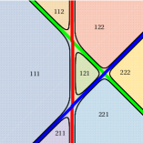
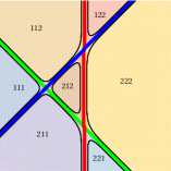
Figure 3: Yang-Baxter relation in terms of vector KP line solitons. These are contour plots in the $xy$-plane (horizontal $x$- and vertical $y$-axis) of a 3-soliton solution at negative, respectively positive $t$. A number $abc$ indicates the respective dominating phase region.

The contour plots in Fig. 3 show the structure at fixed $t$ with $t<0$ and $t>0$, respectively. The lines extending to the bottom are numbered by $1,2,3$ from left to right (displayed as blue, red, green, respectively). Thinking of three particles undergoing a scattering process in $y$-direction, they carry polarizations that change at “crossing points”. As $y$ increases we have

$$(\hat{u}_{111,211},\hat{u}_{211,221},\hat{u}_{221,222})\stackrel{{\scriptstyle 12}}{{\mapsto}}(\hat{u}_{121,221},\hat{u}_{111,121},\hat{u}_{221,222})\stackrel{{\scriptstyle 13}}{{\mapsto}}(\hat{u}_{122,222},\hat{u}_{111,121},\hat{u}_{121,122})$$

$$\stackrel{{\scriptstyle 23}}{{\mapsto}}(\hat{u}_{122,222},\hat{u}_{112,122},\hat{u}_{111,112})$$

for $t<0$, where the $i$-th entry contains the polarization of the $i$-th particle, and

$$(\hat{u}_{111,211},\hat{u}_{211,221},\hat{u}_{221,222})\stackrel{{\scriptstyle 23}}{{\mapsto}}(\hat{u}_{111,211},\hat{u}_{212,222},\hat{u}_{211,212})\stackrel{{\scriptstyle 13}}{{\mapsto}}(\hat{u}_{112,212},\hat{u}_{212,222},\hat{u}_{111,112})$$

$$\stackrel{{\scriptstyle 12}}{{\mapsto}}(\hat{u}_{122,222},\hat{u}_{112,122},\hat{u}_{111,112})$$

for $t>0$. The numbers $ij$ assigned to the steps refer to the “particles” involved. In both cases we start and end with the same vectors, and this implies the Yang-Baxter equation for the associated transformations. Let $V_{a_{1}a_{2}a_{3},b_{1}b_{2}b_{3}}$ be the column vector formed by the coefficients of $\hat{u}_{a_{1}a_{2}a_{3},b_{1}b_{2}b_{3}}$ with respect to $\hat{\xi}_{1},\hat{\xi}_{2},\hat{\xi}_{3}$. The following matrices are composed of these column vectors,

$$U_{123}=\left(\begin{array}[]{ccc}V_{111,211}&V_{211,221}&V_{221,222}\end{array}\right)\,,\quad U_{213}=\left(\begin{array}[]{ccc}V_{121,221}&V_{111,121}&V_{221,222}\end{array}\right)\,,$$

$$U_{231}=\left(\begin{array}[]{ccc}V_{122,222}&V_{111,121}&V_{121,122}\end{array}\right)\,,\quad U_{321}=\left(\begin{array}[]{ccc}V_{122,222}&V_{112,122}&V_{111,112}\end{array}\right)\,,$$

$$U_{132}=\left(\begin{array}[]{ccc}V_{111,211}&V_{212,222}&V_{211,212}\end{array}\right)\,,\quad U_{312}=\left(\begin{array}[]{ccc}V_{112,212}&V_{212,222}&V_{111,112}\end{array}\right)\,.$$

They represent the triplets of polarizations constituting the above chains. Next we define matrices

$$r_{12}=U_{123}^{-1}U_{213}=U_{312}^{-1}U_{321}\,,\quad r_{13}=U_{213}^{-1}U_{231}=U_{132}^{-1}U_{312}\,,\quad r_{23}=U_{231}^{-1}U_{321}=U_{123}^{-1}U_{132}\,,$$

which turn out to be given in terms of the $R$-matrix (5.8). For example,

$$r_{13}=\left(\begin{array}[]{ccc}\frac{p_{1}-p_{3}}{p_{1}-q_{3}}&0&\frac{p_{1}-q_{1}}{p_{1}-q_{3}}\\ 0&1&0\\ \frac{p_{3}-q_{3}}{p_{1}-q_{3}}&0&\frac{q_{1}-q_{3}}{p_{1}-q_{3}}\end{array}\right)\,.$$

The Yang-Baxter equation reads

$$r_{12}\,r_{13}\,r_{23}=r_{23}\,r_{13}\,r_{12}\,.$$

Fig. 4 shows plots of $Ku$ for a choice of the parameters.

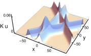
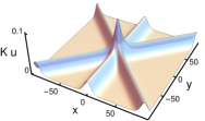
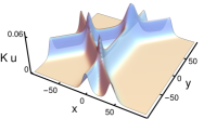
Figure 4: Plots of the scalar $Ku$ for a “Yang-Baxter line soliton configuration” of a vector KP equation at times $t<0$, $t=0$ and $t>0$.

6.2 Vector KdV 3-soliton solutions

We impose the KdV reduction, see Remark 3.4, and replace (2.3) by

$$\vartheta(P)=x\,P+t\,P^{3}+s\,P^{5}\,.$$

The additional last term introduces the next evolution variable $s$ of the KdV hierarchy, also see Remark 2.1.

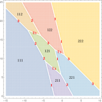
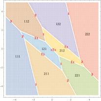
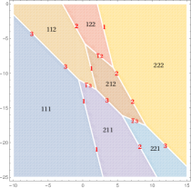
Figure 5: Tropical limit graph and dominating phase regions of a vector KdV solution in two-dimensional space-time ($x$ horizontal, $t$ vertical), at $s=-10$, $s=0$ and $s=10$. See Section 6.2. Numbers $1,2,3$ (in red) attached to lines identify appearances of the respective soliton. Here bounded lines are formally associated with a pair of a (virtual) anti-soliton, indicated by a bar over the respective number, and a (virtual) soliton. At $s=0$, a “composite” of three virtual solitons ($1\bar{2}3$) shows up.

Let us consider, for simplicity, the KdV_K equation with $m=3$ and $K=(1,1,1)$, and the special solution with parameters

$$\theta_{1}=I_{3}\,,\qquad\chi_{1}=(1,-1,1)^{\intercal}\,.$$

The tropical limit graph is displayed in Fig. 5 for $p_{1}=1/2$, $p_{2}=3/4$, $p_{3}=1$, and different values of $s$. We have the matrix

$$U_{123}=\left(\begin{array}[]{ccc}\hat{u}_{111,211}&\hat{u}_{211,221}&\hat{u}_{221,222}\end{array}\right)=\left(\begin{array}[]{ccc}\frac{(p_{1}+p_{2})(p_{1}+p_{3})}{(p_{1}-p_{2})(p_{1}-p_{3})}&0&0\\ -\frac{2p_{2}(p_{2}+p_{3})}{(p_{1}-p_{2})(p_{2}-p_{3})}&\frac{p_{2}+p_{3}}{p_{2}-p_{3}}&0\\ \frac{2p_{3}(p_{2}+p_{3})}{(p_{1}-p_{3})(p_{2}-p_{3})}&-\frac{2p_{3}}{p_{2}-p_{3}}&1\end{array}\right)$$

of initial polarizations. The next values $\hat{u}_{abc,def}$ are then obtained by application of the $R$-matrix (5.11) from the right, and so forth, following either the left or the right graph in Fig. 5 in upwards (i.e., $t$-) direction. Since the initial and the final polarizations are the same, the Yang-Baxter equation holds. Here the $R$-matrix describes the time evolution of polarizations in the tropical limit.

Fig. 5 suggests to think of $R$-matrices as being associated with bounded lines, which may be thought of as representing “virtual solitons”. Interaction of two solitons then means exchange of a virtual soliton.

At $s=0$, see the plot in the middle of Fig. 5, something peculiar occurs, namely a sort of three-particle interaction. This is a degenerate special case to which the Yang-Baxter description does not apply. But this is not relevant for our conclusions.

7 Tropical limit of pure vector solitons and the $R$-matrix

We set $n=1$ (vector case). The following results describe what happens at a “crossing” of two solitons, numbered by $i$ and $j$, depicted as a contour plot in Fig. 6.

Lemma 7.1.

$$(p_{i}-p_{j})\,\phi_{I_{ij}(1,1)}+(q_{i}-q_{j})\,\phi_{I_{ij}(2,2)}=(p_{i}-q_{j})\,\phi_{I_{ij}(1,2)}+(q_{i}-p_{j})\,\phi_{I_{ij}(2,1)}\,.$$ (7.1)

Proof.

This is quickly verified for the 2-soliton solution ($N=2$). But at a crossing a general solution $\phi$ is equivalent to a 2-soliton solution, since there the four elementary phases $\vartheta(p_{i,a}),\vartheta(p_{j,a})$, $a=1,2$, dominate all others, hence the exponential of any other phase vanishes in the tropical limit. ∎

Remark 7.2.

(7.1) can be regarded as a vector version of a scalar linear quadrilaterial equation, satisfying “consistency on a cube”, see (15) in [18]. Such a linear relation does not hold in the matrix case where $m,n>1$. But (5.1), with $\phi_{ab}$ replaced by $\phi_{I_{ij}(a,b)}$ (in which case we have $\phi_{I_{ij}(2,2)}\neq 0$, in general) is a nonlinear counterpart of (7.1). The latter can be deduced from it for $n=1$ by using (4.5). $\square$

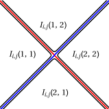
Figure 6: A “crossing” of solitons with numbers $i$ and $j$ at fixed time in the $xy$-plane, and the numbers of the four phases that are involved.

Theorem 7.3.

$$\left(\begin{array}[]{cc}\hat{u}_{I_{ij}(1,1),I_{ij}(2,1)}&\hat{u}_{I_{ij}(2,1),I_{ij}(2,2)}\end{array}\right)R(p_{i},q_{i};p_{j},q_{j})=\left(\begin{array}[]{cc}\hat{u}_{I_{ij}(1,2),I_{ij}(2,2)}&\hat{u}_{I_{ij}(1,1),I_{ij}(1,2)}\end{array}\right)$$ (7.4)

with

$$R(p_{i},q_{i};p_{j},q_{j})=\left(\begin{array}[]{cc}\frac{p_{i}-p_{j}}{p_{i}-q_{j}}&\frac{p_{i}-q_{i}}{p_{i}-q_{j}}\\ \frac{p_{j}-q_{j}}{p_{i}-q_{j}}&\frac{q_{i}-q_{j}}{p_{i}-q_{j}}\end{array}\right)\,.$$

Proof.

Using (4.4) we can directly verify that the following relations hold as a consequence of (7.1),

$$\frac{p_{i}-p_{j}}{p_{i}-q_{j}}\hat{u}_{I_{ij}(1,1),I_{ij}(2,1)}+\frac{p_{j}-q_{j}}{p_{i}-q_{j}}\hat{u}_{I_{ij}(2,1),I_{ij}(2,2)}=\hat{u}_{I_{ij}(1,2),I_{ij}(2,2)}\,,$$

$$\frac{p_{i}-q_{i}}{p_{i}-q_{j}}\hat{u}_{I_{ij}(1,1),I_{ij}(2,1)}+\frac{q_{i}-q_{j}}{p_{i}-q_{j}}\hat{u}_{I_{ij}(2,1),I_{ij}(2,2)}=\hat{u}_{I_{ij}(1,1),I_{ij}(1,2)}\,.$$

In matrix form, this is (7.4). ∎

We already know that $R(p_{i},q_{i};p_{j},q_{j})$ satisfies the Yang-Baxter equation.

8 Construction of pure vector KP soliton solutions from a scalar KP solution and the $R$-matrix

Given a $\tau$-function for a pure $N$-soliton solution of the scalar KP equation, the Yang-Baxter $R$-matrix found above can be used to construct a pure $N$-soliton solution of the vector KP equation. We will explain this for the case $N=3$.

The $\tau$-function of the pure 3-soliton solution of the scalar KP-II equation is given by

$$\tau=\sum_{a,b,c=1}^{2}\Delta_{abc}\,e^{\vartheta_{abc}}\,,\quad\Delta_{abc}=(p_{2,b}-p_{1,a})(p_{3,c}-p_{1,a})(p_{3,c}-p_{2,b})\,,$$

as obtained by the Wronskian method (see, e.g., [19]). Comparison with (3.6) shows that $\mu_{I}=\Delta_{I}$.

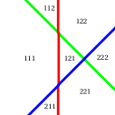
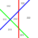
Figure 7: Three-soliton configuration for $t<0$ and $t>0$, respectively, in the $xy$-plane. Numbers specify dominating phase regions.

Starting at the bottom of both graphs in Fig. 7, we associate a column vector $\xi_{i}$ with the $i$-th soliton (counted from left to right) and normalize it such that $K\xi_{i}=1$. Accordingly, we set

$$\hat{u}_{111,211}=\xi_{1}\,,\quad\hat{u}_{211,221}=\xi_{2}\,,\quad\hat{u}_{221,222}=\xi_{3}\,.$$

By consecutive application of the $R$-matrix (5.8), we find the polarizations on the further line segments, proceeding in $y$-direction. There are different ways to proceed, but they are consistent since $R$ satisfies the Yang-Baxter equation. For example,

$$\left(\begin{array}[]{cc}\hat{u}_{121,221}&\hat{u}_{111,121}\end{array}\right)=\left(\begin{array}[]{cc}\hat{u}_{111,211}&\hat{u}_{211,221}\end{array}\right)\,R(p_{1},q_{1};p_{2},q_{2})\,.$$

This leads to

$$\hat{u}_{121,221} = \frac{p_{1}-p_{2}}{p_{1}-q_{2}}\xi_{1}+\frac{p_{2}-q_{2}}{p_{1}-q_{2}}\xi_{2}\,,\qquad\hat{u}_{111,121}=\frac{p_{1}-q_{1}}{p_{1}-q_{2}}\xi_{1}+\frac{q_{1}-q_{2}}{p_{1}-q_{2}}\xi_{2}\,,$$

$$\hat{u}_{212,222} = \frac{p_{2}-p_{3}}{p_{2}-q_{3}}\xi_{2}+\frac{p_{3}-q_{3}}{p_{2}-q_{3}}\xi_{3}\,,\qquad\hat{u}_{211,212}=\frac{p_{2}-q_{2}}{p_{2}-q_{3}}\xi_{2}+\frac{q_{2}-q_{3}}{p_{2}-q_{3}}\xi_{3}\,,$$

$$\hat{u}_{122,222} = \frac{(p_{1}-p_{2})(p_{1}-p_{3})}{(p_{1}-q_{2})(p_{1}-q_{3})}\xi_{1}+\frac{(p_{1}-p_{3})(p_{2}-q_{2})}{(p_{1}-q_{2})(p_{1}-q_{3})}\xi_{2}+\frac{p_{3}-q_{3}}{p_{1}-q_{3}}\xi_{3}\,,$$

$$\hat{u}_{121,122} = \frac{(p_{1}-p_{2})(p_{1}-q_{1})}{(p_{1}-q_{2})(p_{1}-q_{3})}\xi_{1}+\frac{(p_{1}-q_{1})(p_{2}-q_{2})}{(p_{1}-q_{2})(p_{1}-q_{3})}\xi_{2}+\frac{q_{1}-q_{3}}{p_{1}-q_{3}}\xi_{3}\,,$$

$$\hat{u}_{111,112} = \frac{p_{1}-q_{1}}{p_{1}-q_{3}}\xi_{1}+\frac{(p_{2}-q_{2})(q_{1}-q_{3})}{(p_{1}-q_{3})(p_{2}-q_{3})}\xi_{2}+\frac{(q_{1}-q_{3})(q_{2}-q_{3})}{(p_{1}-q_{3})(p_{2}-q_{3})}\xi_{3}\,,$$

$$\hat{u}_{112,212} = \frac{p_{1}-p_{3}}{p_{1}-q_{3}}\xi_{1}+\frac{(p_{2}-q_{2})(p_{3}-q_{3})}{(p_{1}-q_{3})(p_{2}-q_{3})}\xi_{2}+\frac{(p_{3}-q_{3})(q_{2}-q_{3})}{(p_{1}-q_{3})(p_{2}-q_{3})}\xi_{3}\,,$$

$$\hat{u}_{112,122} = \frac{(p_{1}-p_{3})(p_{1}-q_{1})}{(p_{1}-q_{2})(p_{1}-q_{3})}\xi_{1}+\frac{(p_{2}-p_{3})(q_{1}-q_{2})(p_{1}-q_{3})+(p_{1}-q_{1})(p_{2}-q_{2})(p_{3}-q_{3})}{(p_{1}-q_{3})(p_{1}-q_{2})(p_{2}-q_{3})}\xi_{2}$$

$$+\frac{(p_{3}-q_{3})(q_{1}-q_{3})}{(p_{1}-q_{3})(p_{2}-q_{3})}\xi_{3}\,.$$

By “integration” of (4.4), we find $\phi_{abc}$ up to a single constant. Setting $\phi_{222}=0$, we obtain

$$\phi_{111} = \xi_{1}(p_{1}-q_{1})+\xi_{2}(p_{2}-q_{2})+\xi_{3}(p_{3}-q_{3})\,,$$

$$\phi_{112} = \frac{(p_{1}-p_{3})(p_{1}-q_{1})}{p_{1}-q_{3}}\xi_{1}+\Big{(}\frac{(q_{1}-q_{3})(p_{2}-q_{2})(p_{3}-q_{3})}{(p_{1}-q_{3})(q_{3}-p_{2})}+p_{2}-q_{2}\Big{)}\xi_{2}$$

$$+\Big{(}\frac{(q_{1}-q_{3})(q_{2}-q_{3})(p_{3}-q_{3})}{(p_{1}-q_{3})(q_{3}-p_{2})}+p_{3}-q_{3}\Big{)}\xi_{3}$$

$$\phi_{121} = \frac{(p_{1}-p_{2})(p_{1}-q_{1})}{p_{1}-q_{2}}\xi_{1}+\frac{(p_{1}-q_{1})(p_{2}-q_{2})}{p_{1}-q_{2}}\xi_{2}+(p_{3}-q_{3})\xi_{3}\,,$$

$$\phi_{211} = (p_{2}-q_{2})\xi_{2}+(p_{3}-q_{3})\xi_{3}\,,$$

$$\phi_{122} = \frac{(p_{1}-p_{2})(p_{1}-p_{3})(p_{1}-q_{1})}{(p_{1}-q_{2})(p_{1}-q_{3})}\xi_{1}+\frac{(p_{1}-p_{3})(p_{1}-q_{1})(p_{2}-q_{2})}{(p_{1}-q_{2})(p_{1}-q_{3})}\xi_{2}+\frac{(p_{1}-q_{1})(p_{3}-q_{3})}{p_{1}-q_{3}}\xi_{3}\,,$$

$$\phi_{221} = (p_{3}-q_{3})\xi_{3}\,,$$

$$\phi_{212} = \frac{(p_{2}-p_{3})(p_{2}-q_{2})}{p_{2}-q_{3}}\xi_{2}+\frac{(p_{2}-q_{2})(p_{3}-q_{3})}{p_{2}-q_{3}}\xi_{3}\,.$$

From (4.1) we can read off $M_{abc}$ and thus obtain via (3.3) and (3.5) the solution

$$\phi=\frac{1}{\tau}\sum_{a,b,c=1}^{2}M_{abc}\,e^{\vartheta_{abc}}$$

of the vector pKP equation. This procedure can easily be applied to a larger number of solitons.

9 A solution of the tetrahedron equation

In this section we address again the case of three pure solitons, see Section 6. Because of the occurrence of phase shifts, in the tropical limit the “crossing points” of solitons are not really points. Fig. 8 shows this for the second interaction (in the vertical $y$-direction) in Fig. 3, or Fig. 7.

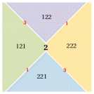
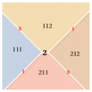
Figure 8: Passing to the tropical limit and zooming into the second interaction “point” in the tropical limit of Fig. 3, shows the tropical origin of phase shifts. Again, the left figure refers to $t<0$, the right to $t>0$.

We may think of associating with the additional edge in the left plot ($t<0$) the polarization of the boundary between the phase regions numbered by $121=(1,2,1)$ and $222$, and in the right plot ($t>0$) that of the boundary between the phases $112$ and $211$. But this does not lead us to something meaningful. Instead, we make an educated guess and associate a mean value of vectors with an additional edge,

$$V_{1}=\frac{1}{2}\left(V_{111,221}+V_{121,211}\right)\,,\quad V_{2}=\frac{1}{2}\left(V_{121,222}+V_{122,221}\right)\,,\quad V_{3}=\frac{1}{2}\left(V_{111,122}+V_{121,112}\right)\,,$$

and

$$\hat{V}_{1}=\frac{1}{2}\left(V_{112,222}+V_{122,212}\right)\,,\quad\hat{V}_{2}=\frac{1}{2}\left(V_{111,212}+V_{112,211}\right)\,,\quad\hat{V}_{3}=\frac{1}{2}\left(V_{211,222}+V_{212,221}\right)\,.$$

The inner boundary lines shown in the two plots in Fig. 8 are now associated with $V_{2}$, respectively $\hat{V}_{2}$. In the first plot, the boundary between phase regions $122$ and $221$ is hidden, but there is also a polarization associated with it, namely $V_{122,221}$. $V_{2}$ is the mean value of the latter and $V_{121,222}$, which belongs to the visible inner boundary segment.

Now we have

$$S(i,j,k)=\left(\begin{array}[]{ccc}V_{1}&V_{2}&V_{3}\end{array}\right)^{-1}\left(\begin{array}[]{ccc}\hat{V}_{1}&\hat{V}_{2}&\hat{V}_{3}\end{array}\right)\Big{|}_{p_{1}\mapsto p_{i},p_{2}\mapsto p_{j},p_{3}\mapsto p_{k},q_{1}\mapsto q_{i},q_{2}\mapsto q_{j},q_{3}\mapsto q_{k}}=\frac{1}{\delta_{ijk}}\gamma^{ijk}-1_{3}\,,$$

where $\gamma^{ijk}=(\gamma^{ijk}_{rs})$ with

$$\gamma^{ijk}_{11}=\rho_{k}\left(\rho_{i}(p_{k}+q_{k}-2q_{i})+\rho_{j}(p_{k}+q_{k}-2p_{j})\right),$$

$$\gamma^{ijk}_{22}=\rho_{j}\left(\rho_{i}(p_{j}+q_{j}-2q_{i})-\rho_{k}(p_{j}+q_{j}-2q_{k})\right),$$

$$\gamma^{ijk}_{33}=-\left(\rho_{i}(\rho_{j}(p_{i}+q_{i}-2p_{j})+\rho_{k}(p_{i}+q_{i}-2q_{k})\right),$$

$$\gamma^{ijk}_{12}=-\rho_{k}\frac{\rho_{i}^{2}-\rho_{j}^{2}}{\rho_{i}^{2}-\rho_{k}^{2}}\left(\rho_{k}^{2}-\rho_{i}(-2q_{i}+p_{k}+q_{k})\right),\quad\gamma^{ijk}_{13}=-\rho_{k}\frac{\rho_{i}^{2}-\rho_{j}^{2}}{\rho_{j}^{2}-\rho_{k}^{2}}\left(\rho_{j}(p_{k}+q_{k}-2p_{j})+\rho_{k}^{2}\right),$$

$$\gamma^{ijk}_{21}=-\rho_{j}\frac{\rho_{i}^{2}-\rho_{k}^{2}}{\rho_{i}^{2}-\rho_{j}^{2}}\left(\rho_{j}^{2}-\rho_{i}(p_{j}+q_{j}-2q_{i})\right),\quad\gamma^{ijk}_{23}=\rho_{j}\frac{\rho_{i}^{2}-\rho_{k}^{2}}{\rho_{j}^{2}-\rho_{k}^{2}}\left(\rho_{j}^{2}-\rho_{k}(p_{j}+q_{j}-2q_{k})\right),$$

$$\gamma^{ijk}_{31}=\rho_{i}\frac{\rho_{j}^{2}-\rho_{k}^{2}}{\rho_{i}^{2}-\rho_{j}^{2}}\left(\rho_{j}(p_{i}+q_{i}-2p_{j})+\rho_{i}^{2}\right),\quad\gamma^{ijk}_{32}=\rho_{i}\frac{\rho_{j}^{2}-\rho_{k}^{2}}{\rho_{i}^{2}-\rho_{k}^{2}}\left(\rho_{i}^{2}-\rho_{k}(p_{i}+q_{i}-2q_{k})\right),$$

and

$$\delta_{ijk}=\left(p_{j}-q_{i}\right)\rho_{i}\rho_{j}+\left(q_{k}-q_{i}\right)\rho_{i}\rho_{k}+\left(q_{k}-p_{j}\right)\rho_{j}\rho_{k}\,.$$

Here we set

$$\rho_{i}=p_{i}-q_{i}\,.$$

Let $S_{\alpha\beta\gamma}(i,j,k)$ be the $6\times 6$ matrix which acts via $S(i,j,k)$ on the positions $\alpha,\beta,\gamma$ of a $6$-component column vector, and as the identity on the others. Let

$$\mathcal{R}_{123}=S_{123}(1,2,3)\,,\quad\mathcal{R}_{145}=S_{145}(1,2,4)\,,\quad\mathcal{R}_{246}=S_{246}(1,3,4)\,,\quad\mathcal{R}_{356}=S_{356}(2,3,4)\,.$$

We verified that this constitutes a (to our knowledge new) solution of the tetrahedron (Zamolodchikov) equation (see e.g. [11] and references cited there)

$$\mathcal{R}_{123}\,\mathcal{R}_{145}\,\mathcal{R}_{246}\,\mathcal{R}_{356}=\mathcal{R}_{356}\,\mathcal{R}_{246}\,\mathcal{R}_{145}\,\mathcal{R}_{123}\,.$$ (9.2)

An explanation for the choices of numbers in the above definition of $\mathcal{R}_{\alpha\beta\gamma}$ can be found in Fig. 9. Also see [14].

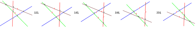
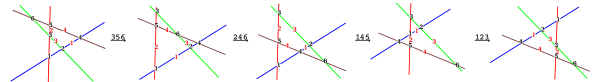
Figure 9: KP line solitons remain parallel while moving. The two chains of line configurations (here shifts are disregarded) show the two different ways in which a 4-soliton solution can evolve from the same initial to the same final configuration. (The two chains represent the higher Bruhat order $B(4,2)$, cf. [11].) This implies the tetrahedron equation. Here (red) numbers attached to lines enumerate the four solitons. Also the crossings of pairs of them are enumerated (by numbers in black). Time evolution proceeds by inversion of triangles. In the first chain, the first step is the inversion of the triangle formed by the crossings numbered $1,2,3$. The second step is the inversion of the triangle formed by the crossings $1,4,5$. The latter involves the solitons with numbers $1,2,4$.

Remark 9.1.

The KdV_K reduction $q_{i}=-p_{i}$ yields

$$S_{\mathrm{KdV}}(i,j,k)=\left(\begin{array}[]{ccc}-\frac{(p_{i}+p_{k})(p_{j}-p_{k})}{(p_{i}-p_{k})(p_{j}+p_{k})}&\frac{2(p_{i}-p_{j})p_{k}}{(p_{i}-p_{k})(p_{j}+p_{k})}&\frac{2(p_{i}-p_{j})p_{k}}{(p_{i}-p_{k})(p_{j}+p_{k})}\\ \frac{2p_{j}(p_{i}+p_{k})}{(p_{i}+p_{j})(p_{j}+p_{k})}&\frac{(p_{i}-p_{j})(p_{j}-p_{k})}{(p_{i}+p_{j})(p_{j}+p_{k})}&\frac{2p_{j}(p_{i}+p_{k})}{(p_{i}+p_{j})(p_{j}+p_{k})}\\ \frac{2p_{i}(p_{j}-p_{k})}{(p_{i}+p_{j})(p_{i}-p_{k})}&\frac{2p_{i}(p_{j}-p_{k})}{(p_{i}+p_{j})(p_{i}-p_{k})}&-\frac{(p_{i}-p_{j})(p_{i}+p_{k})}{(p_{i}+p_{j})(p_{i}-p_{k})}\\ \end{array}\right)\,,$$

which determines a simpler solution of the tetrahedron equation. $\square$

10 A generalization of the vector KP $R$-matrix and a solution of the functional tetrahedron equation

The vector KdV $R$-matrix (5.11) is obtained from the one-parameter $R$-matrix (see, e.g., [13, 14] for a similar $R$-matrix)

$$R(x)=\left(\begin{array}[]{cc}x&1+x\\ 1-x&-x\end{array}\right)\,,$$

by setting $x=(p_{1}-p_{2})/(p_{1}+p_{2})$. The local Yang-Baxter equation

$$R_{12}(x)\,R_{13}(y)\,R_{23}(z)=R_{23}(Z)\,R_{13}(Y)\,R_{12}(X)\,,$$

where indices $\alpha\beta$ indicate on which components of a three-fold direct sum $R$ acts, determines the map $(x,y,z)\mapsto(X,Y,Z)$ given by

$$X=\frac{xy}{x+z-xyz}\,,\quad Y=x+z-xyz\,,\quad Z=\frac{yz}{x+z-xyz}\,.$$

A similar map appeared in [13, 14]. A general argument (cf., e.g., [11] and references cited there) implies that

$$\mathcal{R}(x,y,z):=(X,Y,Z)$$

solves the (functional) tetrahedron equation (9.2), where a “product” of $\mathcal{R}$’s now has to be interpreted as composition of maps. This tetrahedron map is involutive. Setting $x=(p_{1}-p_{2})/(p_{1}+p_{2})$, $y=(p_{1}-p_{3})/(p_{1}+p_{3})$ and $z=(p_{2}-p_{3})/(p_{2}+p_{3})$, it becomes the identity.

Correspondingly, the vector KP $R$-matrix (5.8) is obtained from the more general two-parameter $R$-matrix

$$R(x,y)=\left(\begin{array}[]{cc}x&y\\ 1-x&1-y\end{array}\right)\,,$$

by setting $x=(p_{1}-p_{2})/(p_{1}-q_{2})$ and $y=(p_{1}-q_{1})/(p_{1}-q_{2})$. The local Yang-Baxter equation

$$R_{12}(x,y)\,R_{13}(z,u)\,R_{23}(v,w)=R_{23}(V,W)\,R_{13}(Z,U)\,R_{12}(X,Y)\,,$$

determines the map $(x,y;z,u;v,w)\mapsto(X,Y;Z,U;V,W)$, where

$$X=z\,C\,,\quad Y=(z-\frac{A}{x})\,C\,,\quad Z=\frac{x}{C}\,,$$

$$U=1-B\,,\quad V=\frac{vz\,(x-y)}{A}\,,\quad W=1-\frac{(1-u)(1-w)}{B}\,,$$

with

$$A=uvx-ux-vy+xz\,,\quad B=uwx-ux-wy+1\,,$$

$$C=\frac{AB-A(1-u)(1-w)x-Bv\,(x-y)}{AB-A(1-u)(1-w)-Bvz\,(x-y)}\,.$$

Then

$$\mathcal{R}(x,y;z,u;v,w):=(X,Y;Z,U;V,W)$$

solves the functional (i.e., set-theoretical) tetrahedron equation.

11 Conclusions

In this work we explored “pure” soliton solutions of matrix KP equations in a tropical limit. In case of the reduction to matrix KdV, this consists of a planar graph in (two-dimensional) space-time, with polarizations assigned to its edges. Given initial polarizations, the evolution of them along the graph is ruled by a Yang-Baxter map. For the vector KdV equation, this is a linear map, hence an $R$ matrix. The classical scattering process of matrix KdV solitons resembles in the tropical limit the scattering of point particles in a 2-dimensional integrable quantum field theory, which is characterized by a scattering matrix that solves the (quantum) Yang-Baxter equation.

We have shown that all this holds more generally for KP_K, where the tropical limit at a fixed time $t$ is given by a graph in the $xy$-plane, with polarizations attached to the soliton lines. Moreover, the vector KP case provides us with a realization of the “classical straight-string model” considered in [14]. It should be noticed, however, that KP line solitons in the tropical limit are not, in general, straight because of the appearance of (phase) shifts.

As a side product of our explorations of the tropical limit of pure vector KP solitons, we derived apparently new solutions of the tetrahedron (Zamolodchikov) equation. Whether these solutions are relevant, e.g., for the construction of solvable models of statistical mechanics in three dimensions, has still to be seen.

Another subclass of soliton solutions of the vector KP equation consists of those, for which the support at fixed time is a rooted and generically binary tree in the tropical limit. For the scalar KP equation, this has been extensively explored in [2, 3]. Instead of the Yang-Baxter equation, the pentagon equation (see [11] and references therein) now plays a role in governing corresponding vector solitons. This will be treated in a separate work.

Acknowledgment.

A.D. thanks V. Papageorgiou for a very helpful discussion.

References

[1]
Kodama Y 2017 KP Solitons and the Grassmannians (SpringerBriefs in
Mathematical Physics vol 22) (Singapore: Springer)
[2]
Dimakis A and Müller-Hoissen F 2011 KP line solitons and Tamari lattices
J. Phys. A: Math. Theor.44 025203
[3]
Dimakis A and Müller-Hoissen F 2012 Associahedra, Tamari Lattices and
Related Structures (Progress in Mathematics vol 299) ed
Müller-Hoissen F, Pallo J and Stasheff J (Basel: Birkhäuser) pp 391–423
[4]
Dimakis A and Müller-Hoissen F 2014 KdV soliton interactions: a tropical
view J. Phys. Conf. Ser.482 012010
[5]
Biondini G and Chakravarty S 2006 Soliton solutions of the
Kadomtsev-Petviashvili II equation J. Math. Phys.47
033514–1–033514–26
[6]
Chakravarty S and Kodama Y 2008 Classification of the line-soliton solutions of
KPII J. Phys. A: Math. Theor.41 275209
[7]
Goncharenko V 2001 Multisoliton solutions of the matrix KdV equation Theor. Math. Phys.126 81–91
[8]
Veselov A 2003 Yang-Baxter maps and integrable dynamics Phys. Lett. A314 214–221
[9]
Goncharenko V and Veselov A 2004 New Trends in Integrability and Partial
Solvability (NATO Science Series II: Math. Phys. Chem. vol 132) ed
Shabat A et al. (Dordrecht: Kluwer) pp 191–197
[10]
Tsuchida T 2004 -soliton collision in the Manakov model Progr.
Theor. Phys.111 151–182
[11]
Dimakis A and Müller-Hoissen F 2015 Simplex and polygon equations SIGMA11 042
[12]
Maillet J and Nijhoff F 1989 Integrability for multidimensional lattice models
Phys. Lett. B224 389–396
[13]
Sergeev S 1998 Solutions of the functional tetrahedron equation connected with
the local Yang-Baxter equation for the ferro-electric condition Lett. Math. Phys.45 113–119
[14]
Kashaev R, Korepanov I and Sergeev S 1998 Functional tetrahedron equation Theor. Math. Phys.117 1402–1403
[15]
Chvartatskyi O, Dimakis A and Müller-Hoissen F 2016 Self-consistent sources
for integrable equations via deformations of binary Darboux transformations
Lett. Math. Phys.106 1139–1179
[16]
Suris Y and Veselov A 2003 Lax matrices for Yang-Baxter maps J. Nonl.
Math. Phys.10 223–230
[17]
Kouloukas T 2017 Relativistic collisions as Yang-Baxter maps Phys.
Lett. A381 3445–3449
[18]
Atkinson J 2009 Linear quadrilateral lattice equations and multidimensional
consistency J. Phys. A: Math. Theor.42 454005
[19]
Hirota R 2004 The Direct Method in Soliton Theory (Cambridge Tracts in Mathematics vol 155) (Cambridge: Cambridge University
Press)