Two Dimensional Clustering of Gamma-Ray Bursts using durations and hardness

Abstract

Gamma-Ray Bursts (GRBs) have been traditionally divided into two categories: “short” and “long” with durations less than and greater than two seconds, respectively. However, there is a lot of literature (with conflicting results) regarding the existence of a third intermediate class. To investigate this issue, we carry out a two-dimensional classification using the GRB hardness and duration, and also incorporating the uncertainties in both the variables, by using an extension of Gaussian Mixture Model called Extreme Deconvolution (XDGMM). We carry out this analysis on datasets from two detectors, viz. BATSE and Fermi-GBM. We consider the duration and hardness features in log-scale for each of these datasets and determine the best-fit parameters using XDGMM. This is followed by information theoretic criterion-based tests (AIC and BIC) to determine the optimum number of classes. For BATSE, we find that both AIC and BIC show preference for two components with close to decisive and decisive significance, respectively. For Fermi-GBM, AIC shows preference for three components with decisive significance, whereas BIC does not find any significant difference between two and three components. Our analysis codes have been made publicly available.

Keywords GRB Classification; Bayesian Information Criterion; Akaike Information Criterion

1 Introduction

Gamma-ray bursts (GRBs) are short-duration energetic cosmic explosions with prompt emission between keV-GeV energies, which are being continuously detected at the rate of about one per day  (Kumar & Zhang, 2015; Zhang et al., 2016a; Schady, 2017). They are located at cosmological distances, although a distinct signature of cosmological time dilation in the GRB light curves remains elusive (Singh & Desai, 2022). The first convincing case for bifurcating the GRB population into two categories was made from an analysis of the BATSE data (Kouveliotou et al., 1993), and led to establishing the conventional classification of GRBs into short (T90 $<$ 2 s) and long (T90 $>$ 2 s) classes, where T90 is the time which encompasses 90% of the burst’s fluence, and is usually used as a proxy for the duration of a GRB. Note however that this boundary between short and long GRBs is known to be detector dependent (Bromberg et al., 2013; Tarnopolski, 2015b). Short GRBs are usually associated with binary neutron star (or other compact object) mergers (Nakar, 2007) and long GRBs with core collapse supernovae (Woosley & Bloom, 2006). However, there are known exceptions to the above general picture (Zhang et al., 2009; Perna et al., 2018; Amati, 2021; Ahumada et al., 2021).

Despite the conventional wisdom of only two distinct GRB classes, multiple groups have argued over the years for the existence of an intermediate class of GRBs in between the short and long bursts, using T90 as the criterion for classification. The first such claim for an intermediate-duration GRB class, with T90 in the range between 2 and 10 seconds in the BATSE dataset was put forward by  Horváth (1998) and Mukherjee et al. (1998), and subsequently confirmed by the analysis of the complete BATSE dataset  (Horváth, 2002; Chattopadhyay et al., 2007a; Tóth et al., 2019).

However, this has been disputed by  Zitouni et al. (2015), who found that two lognormal distributions fit the BATSE T90 data much better compared to three components. Evidence for a third lognormal component was also found in the BAT data of Neil Gehrels SWIFT Observatory (Swift, hereafter)  (Horváth et al., 2008; Zhang & Choi, 2008; Huja et al., 2009; Horváth et al., 2010; Horváth & Tóth, 2016; Zitouni et al., 2015; Tarnopolski, 2016b; von Kienlin et al., 2014). However, these results have been disputed by other authors, who found that the T90 distribution prefers two components (Zhang et al., 2016b; Tarnopolski, 2019b).  Kulkarni & Desai (2017) carried out a unified classification of the T90 distributions for the GRB datasets from BATSE, Fermi, Swift, and Beppo-Sax, and found that among these, only for Swift GRBs in the observed frame is the evidence for three classes marginally significant at about $2.4\sigma$. However, when the same analysis is done for the Swift GRBs in the intrinsic GRB frame, two components are preferred. For all other datasets, evidence for three components is either very marginal or disfavored. Some other works have pointed out that the third component could be an artifact of the skewness in the distribution of long GRBs. If the data is modelled using skewed distributions, only two distributions are sufficient (Tarnopolski, 2016a; Kwong & Nadarajah, 2018; Tarnopolski, 2019b, a).

Extension of studies on GRB classification using both duration and hardness, as well as in dimensions greater than two have also not reached a common consensus. Horváth et al. (2006) and  Chattopadhyay et al. (2007a) argued for three components in the BATSE GRB data using two-dimensional clustering in T90-hardness and T90-fluence planes respectively.  Chattopadhyay & Maitra (2017, 2018) have argued for five components in the BATSE data by using multiple clustering techniques on six different variables. For Swift data, Veres et al. (2010) showed using multiple clustering techniques that three components are favored in the two dimensional $\log$(T90) -$\log$ (hardness) plane, and the intermediate class has overlap with X-ray flashes. However, these results are in conflict with more recent analysis by  Yang et al. (2016), who showed by applying two dimensional Gaussian Mixture Models (GMM) on T90 and hardness ratio on Swift GRBs, that the data favor only two components instead of three. Most recently,  Tarnopolski (2022) showed by applying graph theory techniques to GRB hardness and duration, that the data is consistent with two groups, although a third group cannot be ruled out. Using linear discriminant analysis, Zhang et al. (2022) showed that a linear combination of the duration, fluence, and peak flux is a better discriminant between long and short bursts for Fermi-GBM data. They also showed that long GRBs could also be further sub-divided into long-bright GRBs and long-faint GRBs (Zhang et al., 2022). A recent summary of all results on GRB classification can be found in  Tarnopolski (2019c). Most recently, Swift GRBs have also been classified into categories based entirely on prompt light curves (Jespersen et al., 2020).

To resolve this imbroglio, we use two-dimensional clustering in the hardness vs T90 plane to find out the optimum number of GRB classes. One difference compared to all previous works on GRB classification is that we incorporate the uncertainties in the GRB hardness and T90, while doing the classification. We apply an extension of the GMM, which incorporates the uncertainties in the data (Bovy et al., 2011). We then uniformly apply this method to the latest available GRB data from BATSE and Fermi-GBM detectors, based on the observed T90 and hardness along with their associated uncertainties.

For model comparison, we use two widely used information theoretic criteria, viz. Akaike Information Criterion (AIC) and Bayesian Information Criterion (BIC). Both of these information-criterion based model comparison techniques have been applied to a variety of problems in astrophysics and particle physics, including in the classification of GRBs (Shi et al., 2012; Desai & Liu, 2016; Desai, 2016; Kulkarni & Desai, 2017; Ganguly & Desai, 2017; Kulkarni & Desai, 2018; Krishak & Desai, 2019; Krishak et al., 2020; Krishak & Desai, 2020a, b) and references therein.

The outline of this paper is as follows. The datasets used for our analysis are described in Sect 2. The analysis methodology and model comparison techniques are outlined in Sect. 3. We then present our results for the various GRB datasets in Sect. 4, including a very brief comparison with previous results. We conclude in Sect. 5.

2 Datasets

Herein, we consider the GRB datasets available from BATSE (Paciesas et al., 1999) and Fermi-GBM (Narayana Bhat et al., 2016; von Kienlin et al., 2020). Among these, Fermi detector is still online and detecting on the order of about one new GRB per day. We did not consider other catalogs such as those from Beppo-Sax and INTEGRAL, since they either contained a very small sample of GRBs or did not have any publicly available data for the hardness of the observed bursts. We did not consider the bursts from RHESSI, as it has no onboard GRB triggering mechanism. Although there have been many previous works which used the Swift GRB catalog for classification (Horváth et al., 2008; Horváth & Tóth, 2016; Zhang et al., 2016b; Kulkarni & Desai, 2017), we note that Swift is much more sensitive in the softer bands, meaning that the short GRBs are under-abundant in the sample, which affects the fits (Band, 2006). The selection effects for Swift are therefore difficult to account for (Coward et al., 2013). Therefore, we do not use the data from Swift for our analysis. Before describing each of these datasets, we first explain how the hardness variable was estimated.

2.1 Hardness Definition

Spectral hardness (also referred to as hardness ratio) ($H_{obs}$, hereafter) of a GRB is defined as the ratio between the GRB fluences in different energy bands. For BATSE, we use $H_{obs}$ as the ratio between the $50-100$ keV and the $20-50$ keV bands. The BATSE catalog provides errors for the fluence in both these bands. From this, one can estimate the error in $\log(H_{obs})$ from error propagation. For Fermi-GBM, we consider the ratio of the fluences in 50-300 keV and 10-50 keV to calculate the hardness. We have obtained the errors in hardness and T90 from the latest Fermi-GBM catalog (Narayana-Bhat, private communication, 2020).

Note that many previous works have used BATSE fluences in the 100-300 and 50-100 keV bands for the hardness ratio (Mukherjee et al., 1998; Horváth et al., 2006; Chattopadhyay et al., 2007a; Tarnopolski, 2019c; Tóth et al., 2019). Here, instead we used the fluences in the 20-50 keV energy range in the denominator of the hardness ratio, in order to have overlap in a similar energy range as Fermi-GBM (10-50 keV). Although, we are not analyzing Swift data in this work, clustering studies based on hardness with Swift have also used a similar energy band (25-50 keV) (Zhang et al., 2016b). Therefore, choosing the BATSE fluence in the 20-50 keV range easily allows us to compare with the results from other detectors and also complement the above studies which have used the fluences in 100-300 keV energy range.

2.2 BATSE dataset

The current BATSE GRB (Paciesas et al., 1999) catalog contains 2041 GRBs detected between 1991 and 2000 with duration information and a total of 2035 events with flux and fluence information. Among these, 1973 GRBs contained both duration and fluence information, of which we omitted 39 GRBs for which the fluences in either the 20-50 keV or in the 50-100 keV were less than or equal to zero. Therefore, we are left with 1934 GRBs for our classification purposes. The average fractional error in T90 is 18%, whereas the average fractional error for the fluence in the 50-100 keV and 20-50 keV energy bands is equal to 12% and 17%, respectively.The average and median fractional error in the hardness ratio is 36% and 10%, respectively.

2.3 Fermi-GBM dataset

As of June 2020, Fermi-GBM released their fourth catalog containing 2356 GRBs (Gruber et al., 2014; von Kienlin et al., 2014; Narayana Bhat et al., 2016; von Kienlin et al., 2020). Among these, T90, hardness ratio (as defined above), along with their associated uncertainties are available for 2330 GRBs. Of these, we used 2329 GRBs for analysis, since one GRB had negative value for the hardness and hence could not be used for the analysis. The hardness ratio was calculated using the ratio of the background subtracted flux spectrum (using photon counts) in 50-300 keV to that in 10-50 keV, and averaging over the detectors. More details on this catalog can be found in  von Kienlin et al. (2020). The average fractional error in T90 and hardness ratio is equal to 10% and 18%, respectively. The median fractional error in the hardness ratio is equal to 3%.

3 Methodology

Extreme Deconvolution (XDGMM, hereafter) is an extension of GMM (Kuhn & Feigelson, 2017), which takes into account the uncertainty in the observed data (Bovy et al., 2011; Ivezić et al., 2014; Holoien et al., 2017). It has been used for a variety of applications in astrophysics such as velocity distribution from Hipparcos data (Bovy et al., 2011), classification of pulsars (Reddy Ch. & Desai, 2022), the three-dimensional motions of the stars in Sagittarius streams  (Koposov et al., 2013), classification of neutron star masses (Keitel, 2019), detection of dark matter subhalo candidates (Coronado-Blázquez et al., 2019). We provide a brief description of the XDGMM method using the same notation as  Reddy Ch. & Desai (2022).

We assume that the noisy dataset $x_{i}$ is related to the true values $v_{i}$ as follows (Bovy et al., 2011; Ivezić et al., 2014):

$$x_{i}=R_{i}v_{i}+\epsilon_{i},$$ (1)

where $R_{i}$ is the rotation matrix used to transform the correct values to the observed noisy dataset. Similar to ordinary GMM, we assume that the probability density of the true values $v$ can be written as a mixture of $K$ Gaussians given by

$$p(v_{i})=\sum_{j=1}^{K}\alpha_{j}\mathcal{N}(v_{i}|\mu_{j},\Sigma_{j})$$ (2)

where $\mu_{j}$ and $\Sigma_{j}$ denote the means and variances of each of the Gaussian distribution, whereas $\alpha_{j}$ denotes the weight of each Gaussian subject to $\sum\limits_{j=1}^{K}\alpha_{j}=1$. Note that $x_{i}$ and $v_{i}$ could be multi-dimensional vectors, and for our example, denote the 2-D dataset comprising of the natural logarithms of T90 and $H_{obs}$. We consider the noise $\epsilon_{i}$ (in Eq. 1) to be a Gaussian random variable with zero mean and variance equal to $S_{i}$. The likelihood of the model parameters ($\theta\equiv$ {$\alpha$, $\mu$, $\Sigma$, $R_{i}$, $S_{i}$}) for each noisy data point ($x_{i}$) can then be written as (Bovy et al., 2011):

$$p(x_{i}|\theta)=\sum_{j=1}^{K}\alpha_{j}\mathcal{N}(x_{i}|R_{i}\mu_{j},R_{i}\Sigma_{j}R_{i}^{T}+S_{i})$$ (3)

The last step in XDGMM is to maximize the likelihood of the dataset with respect to the model parameters. This can be done (as in GMM) by adding the individual log-likelihood functions:

$$\underset{\theta}{\operatorname{argmax}}\;L=\sum_{i=1}^{N}\ln(p(x_{i}|\theta)),$$ (4)

where $N$ is the total number of datapoints. This objective function is maximized using an extension of the Expectation-maximization algorithm (Bovy et al., 2011). Similar to GMM, XDGMM returns a likelihood, which can then be utilized for model comparison.

3.1 Fitting method

We now apply XDGMM to the GRB dataset using the $\log$ (T90) and $\log H_{obs}$ as inputs, where $\log$ refers to natural log. We use the XDGMM implementation in the astroML module (Ivezić et al., 2014). We stack the $\log$ (T90) and $\log(H_{obs})$. Their uncertainties constitute the diagonal elements of their respective covariance matrices, with non-diagonal elements kept at zero, since the errors between different GRBs are independent. The stacked covariance matrices are fed to the XDGMM algorithm, whose output consists of the weights, means, and covariances for the input number of clusters

XDGMM by itself does not determine the optimum number of GRBs, which is an input parameter to the algorithm. For finding the optimum number of components, we apply XDGMM by varying the number of GRB components, and then use model selection techniques, as discussed in the next section to determine the optimum number of clusters.

The comparison of models based on the difference in likelihood after finding the best-fit parameters for each model is not the optimum way to find the correct number of components, even though this has been used in the GRB classification literature (Horváth et al., 2006, 2010). For mixture models, minus twice log of difference in likelihood does not asymptote to the usual $\chi^{2}$ distribution (Ghosh & Sen, 1984; Kuhn & Feigelson, 2017). Only when the variances are equal does this statistic follow the $\chi^{2}$ distribution (Kuhn & Feigelson, 2017).

Furthermore, even though the value of the likelihood increases, the addition of extra free parameters leads to increased model complexity and is generally undesired. Therefore, the additional free parameters need to be penalized or taken into account so as to avoid overfitting. To address these issues, a number of both frequentist and Bayesian model-comparison techniques have been used over the past decade to determine the best model which fits the observational data (Liddle, 2004, 2007; Lyons, 2016; Kerscher & Weller, 2019; Krishak & Desai, 2020b). Here, we use information criteria based tests such as AIC and BIC for model comparison, since these are straightforward to compute from the likelihoods (which are returned as one of the outputs from XDGMM). AIC/BIC have also been previously used for GRB classification by a number of authors (Mukherjee et al., 1998; Tarnopolski, 2016a, b; Yang et al., 2016; Kulkarni & Desai, 2017; Tarnopolski, 2019b; Zhang et al., 2022). More information about AIC and BIC and its application to astrophysical problems can be found in  Liddle (2004, 2007); Sharma (2017); Krishak & Desai (2020b).

3.2 AIC

The AIC is used for model comparison, when we need to penalize for any additional free parameters to avoid overfitting. A preferred model in this test is the one with the smaller value of AIC between the two hypothesis. The AIC is given by,

$$AIC=2p-2\ln L.$$ (5)

where $p$ is the number of free parameters in the model and $L$ is the likelihood. The second term favors models with high value of likelihood, while the first term penalizes models which uses large number of parameters. Models with large number of parameters might have a high likelihood but will over fit on the data. The absolute value of AIC is usually not of interest. The goodness of fit between two hypothesis (A) and (B) is described by the difference of the AIC values and is given by,

$$\Delta AIC=AIC_{A}-AIC_{B},$$ (6)

where $AIC_{A}$ - $AIC_{B}$ correspond to the AIC values for the hypothesis A and B. Burnham & Anderson (2004) have provided qualitative strength of evidence rules to assess the significance of a model based on the $\Delta$AIC values between the two models. $\Delta$ AIC$<2$ corresponds to substantial support, those with $4\leq\Delta$AIC$\leq 7$ have considerably less support, and those with $\Delta$AIC have virtually no support. Therefore, $\Delta$AIC$>10$ is considered as decisive evidence against the model with higher AIC (Liddle, 2007; Krishak & Desai, 2020b).

3.3 BIC

The BIC is also used for penalizing the use of extra parameters. As in the case of AIC, the model with the smaller value of BIC is the preferred model. The penalty in the BIC test is harsher than that in the case of AIC and is given by,

$$BIC=p\ln N-2\ln L.$$ (7)

The first term in Eq. 7 acts as a very harsh measure needed for the BIC test. The goodness of fit used for hypothesis testing between two models $A$ and $B$ is given by,

$$\Delta BIC=BIC_{A}-BIC_{B}.$$ (8)

Similar to AIC, the model with lower value of BIC is favored. To assess the significance of a model, strength of evidence rules have also been proposed based on $\Delta$BIC using Jeffreys scale (Kass & Raftery, 1995; Liddle, 2007). $\Delta$ BIC $>5$ is considered as strong evidence and $\Delta$ BIC $>10$ is considered as decisive evidence in favor of the model with the smaller BIC value.

4 Results

We apply the techniques discussed in the previous sections to the GRB datasets from BATSE and Fermi-GBM. We find the mean value of $\log$ (T90) and $\log(H_{obs})$ and its standard deviation for each GRB class, by varying the total number of components from one to five, followed by maximizing the likelihood using XDGMM for each of the hypothesis. This choice for the number of GRB components is large enough, as it allows to easily discern the minimum value of AIC/BIC and also allows us to cross-check the results of some works, which have found upto 5 GRB components (Chattopadhyay & Maitra, 2017, 2018). Using these best-fit parameters, we then implement the information criterion based model-comparison techniques to determine the optimum number of components

4.1 BATSE

A complete summary of the results on applications of XDGMM to the BATSE GRB dataset, including the best-fit parameters and their covariance matrices are shown in Table 1. While fitting for two components, we find that 808 and 1126 GRBs belong to the short and long category respectively. When we fit for three components we find a total of 689, 762, and 483 GRBs in the short, intermediate, and long categories respectively. The AIC and BIC plots as a function of the number of components can be found in Fig. 1. Here, both AIC and BIC prefer two components. The $\Delta$BIC value crosses the threshold of 10, needed for decisive evidence. The $\Delta$AIC value is also close to 10. Therefore, both AIC and BIC results using XDGMM are broadly in agreement and favor two GRB categories. The $1\sigma$ ellipses for two and three components can be found in Fig. 2 and Fig. 3, respectively.

There is more than 20 years of literature on classification of BATSE GRBs. However, the results from different works are not in accord with each other, with disparate statistical techniques often leading to opposite conclusions. So, we only compare our results to a few selected papers, where both T90 and hardness (or other fluence related parameters) are used for classification. Results of classification of BATSE GRBs using only T90 are summarized in  Kulkarni & Desai (2017). The first cogent case for three GRB classes in BATSE data using spectral information, was made by  Chattopadhyay et al. (2007b), who used two multivariate clustering methods using $K$-means partitioning and Dirichlet mixture modeling using fluence vs T90 to argue for three components. However, no estimate of the significance was made. Around the same time, an analysis similar to this using GMM in the log (T90)- log( $H_{obs}$) plane was done by  Horváth et al. (2006), who found that three components were favored using frequentist model comparison by evaluating chi-square probability with the addition of the third component. They also found an anti-correlation between the duration and the hardness. Most recently,  Tarnopolski (2019c) caried out multi-variate modelling of BATSE data using symmetric as well as skewed distributions. He showed that the T90 distribution is consistent with two components. In two dimensional space, almost all the distributions are consistent with two components, except when flux was used for classification in which case, the distribution was well-fitted by three-component Gaussian or $t$-distributions. A comprehensive summary of their classification results in higher-dimensional spaces can be found in Table 1 of  Tarnopolski (2019c). This work argued that it is not possible to unequivocally prove the existence of a third GRB component, since the third component could be a spurious artifact caused by the finite size of the sample and due to a particular realization of the random sample that could bias the results.

The results from our analysis, which incorporates the errors in T90 and $H_{obs}$ support two classes.

Table 1 : Results from model comparison for BATSE GRBs. The first column contains the total number of GRB classes. The two component array ($\log$ T90, $\log H_{obs}$) in the second column denotes the best-fit values for the mean value of the logarithm of T90 (in seconds) and the logarithm of $H_{obs}$. The $2\times 2$ matrix in the third column indicates the covariance matrix $\Sigma$ returned by XDGMM. The fourth column ($n_{i}$) denotes the total number of GRBs. These columns have been shown separately for two and three classes of GRBs. The next set of columns show the AIC and BIC values for each GRB category. The last two columns indicate the $\Delta$AIC, and $\Delta$BIC between the three component and two-component model, which are used for model comparison. In this table, the preferred value for every test is highlighted in bold. We note that $\Delta$AIC = AIC (2 components) - AIC (3 components) and same for $\Delta$BIC. Therefore, if $\Delta$AIC or $\Delta$BIC$>0$, then two GRB classes are preferred and vice-versa. We note that AIC and BIC prefer two components with near decisive and decisive significance, respectively.

$k$	$\mu$	$\Sigma$	$n_{i}$	AIC	BIC	$\Delta(AIC)$	$\Delta(BIC)$
2	(3.08,0.22)	$\left(\begin{array}[]{cc}0.8078&0.0026\\ 0.0026&0.1565\\ \end{array}\right)$	1126	36643.6	36704.9	-9.5	-42.9
	(-0.29,0.52)	$\left(\begin{array}[]{cc}1.6557&-0.1494\\ -0.1494&0.4862\\ \end{array}\right)$	808
3	(2.12,0.20)	$\left(\begin{array}[]{cc}1.0358&0.0936\\ 0.0936&0.3560\\ \end{array}\right)$	762	36653.1	36747.7
	(-0.54,0.61)	$\left(\begin{array}[]{cc}1.3979&-0.0453\\ -0.0453&0.3925\\ \end{array}\right)$	689
	(3.40,0.21)	$\left(\begin{array}[]{cc}0.5599&-0.0021\\ -0.0021&0.1134\\ \end{array}\right)$	483

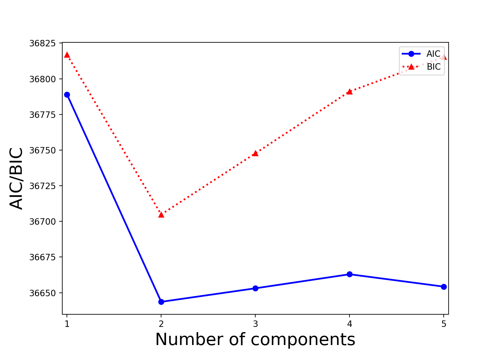
Fig. 1 : AIC and BIC values as a function of the number of Gaussian components for BATSE data after two-dimensional clustering. Both AIC and BIC favor two components with near decisive or decisive significance, respectively.

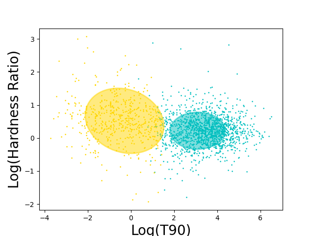
Fig. 2 : Scatter plot of $\log H_{obs}$ vs $\log$ (T90) (expressed in seconds) for BATSE data. The ellipses indicate the 1$\sigma$ contours for two components, using our XDGMM based analysis and are centered on the best-fit parameters obtained from Table 1.

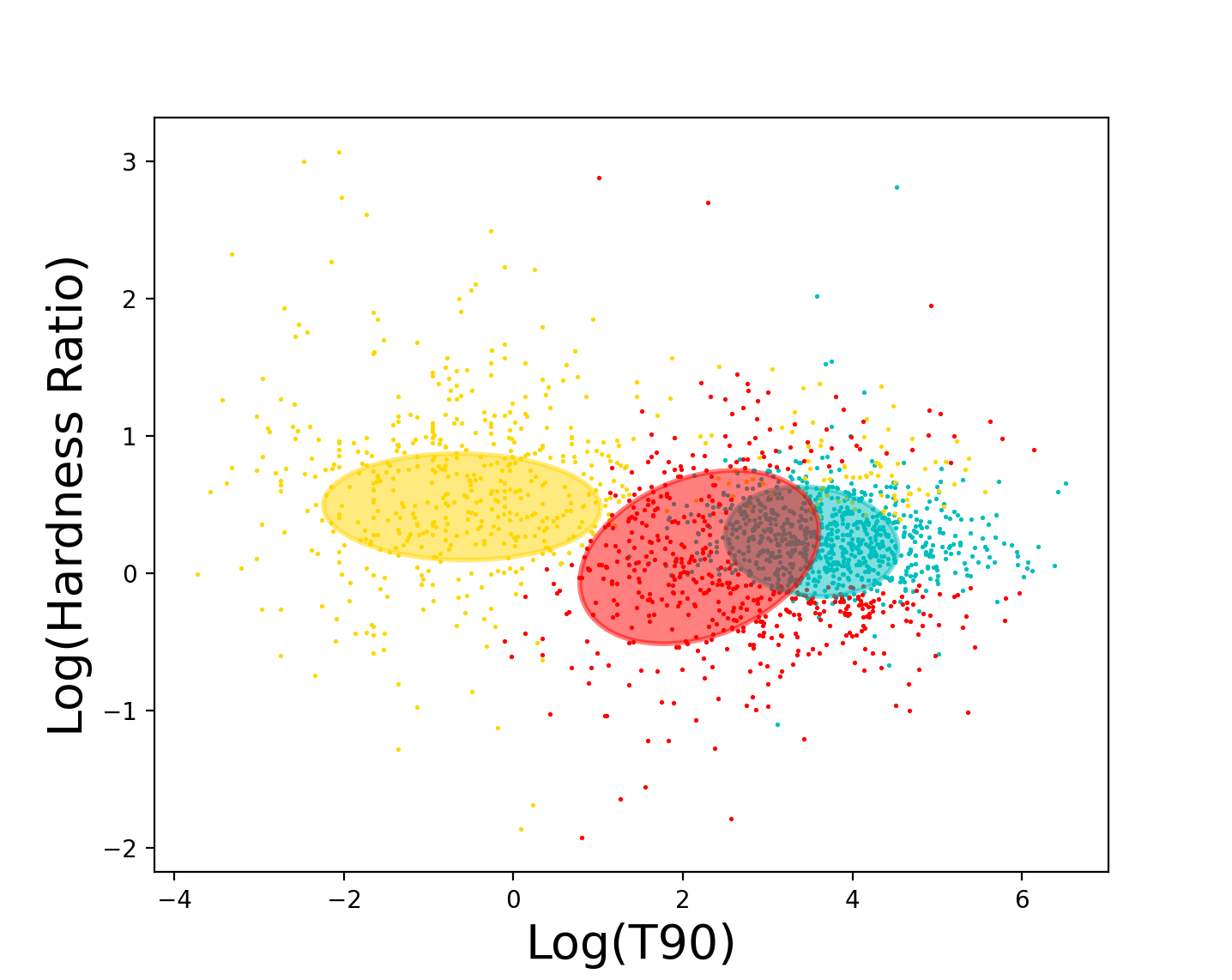
Fig. 3 : Scatter plot of $\log(H_{obs})$ ratio vs $\log$ (T90) (expressed in seconds) for BATSE data. The ellipses indicate the 1$\sigma$ contours from our XDGMM based analysis assuming three components and centered on the best-fit parameters obtained from Table 1.

4.2 Fermi-GBM

A complete summary of the results on applications of XDGMM for Fermi-GBM data, including the best-fit parameters and their covariance matrices are shown in Table 2. For two components, we find that 360 and 1969 GRBs belong to the short and long categories, respectively. For a three component model, we obtain 990, 268, and 1071 GRBs in short, intermediate and long GRB categories respectively. The AIC and BIC plots as a function of the number of GRB components can be found in Fig. 4. The minimum value of AIC is obtained for three components, whereas for BIC the minimum value is obtained for two components. The $\Delta$ AIC values between two and three components is greater than 10, thus pointing to decisive significance in favor of three components. We note that the AIC values for four and five components are also smaller compared to that for two components by more than 10, which implies that four and five components are decisively favored compared to two. However, they are greater than the AIC value for three components by more than 10, implying that AIC shows decisive significance for three components as compared to any other number of components. However, the $\Delta$BIC value between the two and three components is less than three, indicating that the difference is negligible and corresponds to “not worth a mention” according to Jeffreys’ scale. Note however that as discussed in  Tarnopolski (2019c) and  Tarnopolski (2019b), AIC is liberal in overfitting with a higher chance of accepting complicated models having redundant components, than necessary. Therefore, BIC results are more trustworthy in case of a discrepancy between the two. The $1\sigma$ ellipses for the two components are shown in Fig. 5. The corresponding plot for three components can be found in Fig. 6.

Similar to BATSE, there is a vast amount of literature on the classification of Fermi-GBM GRBs, with no common consensus among the different works. We summarize the results from some of these works and then compare with our results. A summary of previous results on the classification of Fermi-GBM using durations can be found in  Kulkarni & Desai (2017); Zitouni et al. (2018). All previous classification studies with Fermi GRBs show a preference for two GRBs. While this work was in progress, a short GRB detected by Fermi-GBM (GRB170817A) (Goldstein et al., 2017) was seen in gravitational waves (GW170817) (Abbott et al., 2017) creating a watershed event in the history of astronomy, and thereby opening the era of multi-messenger astronomy and providing a whole bunch of information from Astrophysics to fundamental Physics (Margutti & Chornock, 2021; Boran et al., 2018). Subsequently, when a clustering analysis of the GRBs from the Fermi-GBM catalog was done using multi-dimensional clustering followed by model selection using BIC, the optimum number of clusters detected was equal to three (Horváth et al., 2018). They have also argued that GRB170817A belongs to an intermediate class and not a short hard burst. A follow-up cluster analysis was carried out by  Horváth et al. (2019) using 16 Fermi-GBM observables, who showed using Principal Component Analysis that the data is consistent with three GRB classes. However, the third class is different from the intermediate class. They argue that this could be caused due to the model-dependent spectral fitting parameters provided by Fermi-GBM.  Tarnopolski (2019b) carried out a 2-d classification using hardness and duration, and showed that the duration–hardness ratio plane is best represented by a mixture of two skewed Student $t$ distributions.  Tarnopolski (2022) showed using graph theory that the Fermi-GBM dataset is consistent with both two and three classes. Most recently, Zhang et al. (2022) showed using linear discriminant analysis that a linear combination of the duration, fluence, and peak flux is a better discriminant between long and short bursts for Fermi-GBM data. They also showed that long GRBs could also be divided into long-bright GRBs and long-faint GRBs (Zhang et al., 2022).

Our analysis indicates that AIC decisively prefers three components, whereas for BIC the difference between the values for two and three components is negligible.

Table 2 : Model comparison parameters for Fermi-GBM GRBs. The explanation of all the columns is same as in Table 1. We find that both AIC prefers three components with decisive significance, whereas BIC prefers two components albeit with marginal difference with respect to the three component model. The AIC value for four and five components is equal to 12952 and 12954 respectively, indicating that four/five classes are favored compared to two, but disfavored when compared to three.

$k$	$\mu$	$\Sigma$	$n_{i}$	AIC	BIC	$\Delta(AIC)$	$\Delta(BIC)$
2	(3.27,-0.46)	$\left(\begin{array}[]{cc}1.11&-0.04\\ -0.04&0.28\\ \end{array}\right)$	1969	12973.5	13036.8	32.3	-2.2
	(-0.09,0.34)	$\left(\begin{array}[]{cc}0.97&-0.19\\ -0.19&0.23\\ \end{array}\right)$	360
3	(3.71,-0.46)	$\left(\begin{array}[]{cc}0.6334&-0.1730\\ -0.1730&0.1744\\ \end{array}\right)$	1071	12941	13039
	(-0.43,0.44)	$\left(\begin{array}[]{cc}0.6334&-0.1730\\ -0.1730&0.1744\\ \end{array}\right)$	990
	(2.59,-0.41)	$\left(\begin{array}[]{cc}1.2993&-0.1167\\ -0.1167&0.4048\\ \end{array}\right)$	268

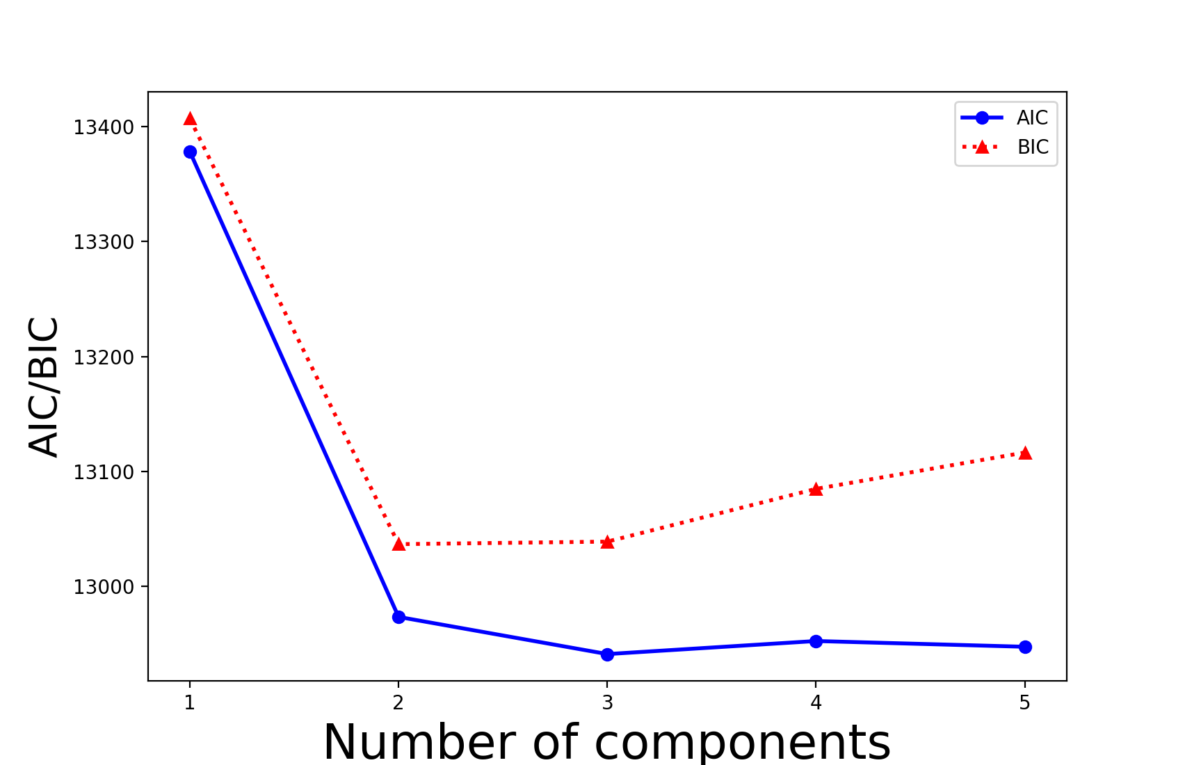
Fig. 4 : AIC and BIC values as a function of the number of Gaussian components for Fermi-GBM data after two-dimensional clustering. The minimum value of BIC is obtained for two components. However the difference compared to the same for three components is negligible. For AIC, the minimum value is obtained for three components and the difference with respect to two components points to decisive significance in favor of the three component model.

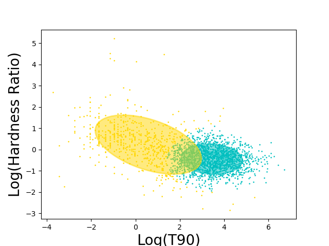
Fig. 5 : Scatter plot of $\log(H_{obs})$ ratio vs $\log$ (T90) (expressed in seconds) for Fermi-GBM data. The ellipses indicate the 1$\sigma$ contours from our XDGMM based analysis assuming two components, using the best-fit results tabulated in Table  2.

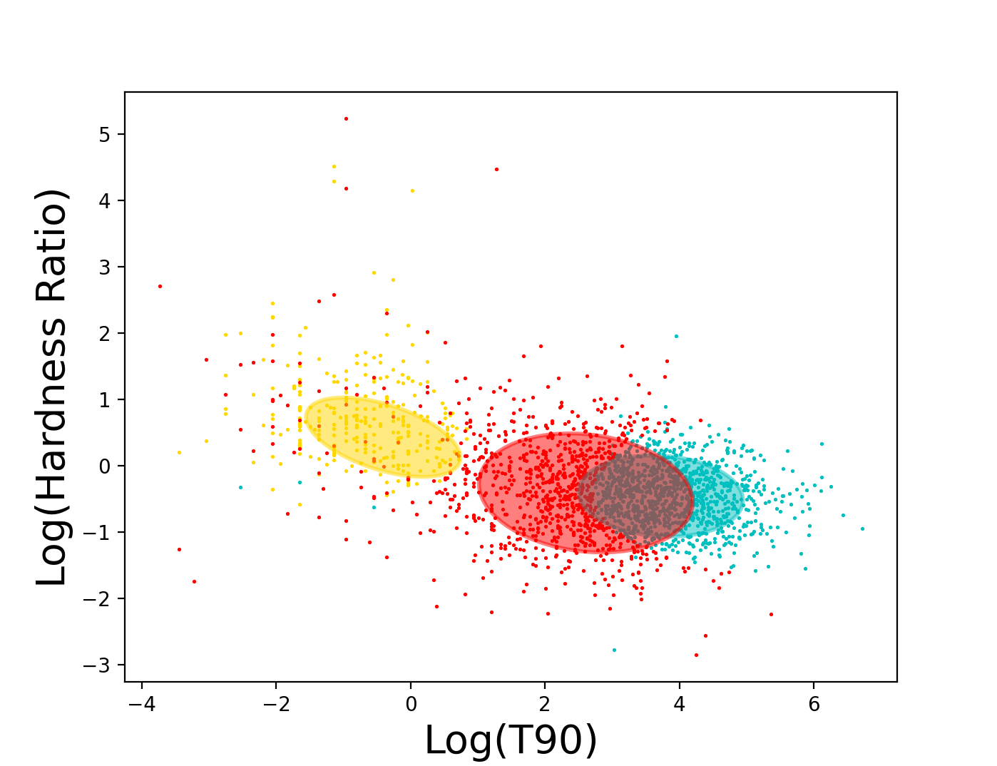
Fig. 6 : Scatter plot of $\log H_{obs}$ ratio vs $\log$ (T90) (expressed in seconds) for Fermi-GBM data. The ellipses indicate the 1$\sigma$ contours from our XDGMM based analysis assuming three components and using the best-fit parameters from Table 2.

Table 3 : Summary of model comparison tests for the GRB datasets analyzed. For each dataset we have indicated the preferred model based on the difference between the values of the AIC and BIC between the best component and the one with the higher value.

Dataset	$\Delta AIC$		$\Delta BIC$
	Optimum Classes	Difference	Optimum Classes	Difference
BATSE	2	9.5	2	42.9
Fermi	3	32.3	2	2.2

5 Conclusions

The main goal of this work was to find the optimum number of GRB components by carrying out a two-dimensional clustering in the T90 vs hardness plane, along with incorporating the errors in T90 and hardness in the aforementioned analysis. Although there are a plethora of works over a time span of more than two decades, which have done a multidimensional classification using multiple GRB observables, none of them have incorporated the uncertainties in the analysis. This is the first work on GRB classification which has included the aforementioned uncertainties. For our analysis, we used an extension of the GMM based classification which incorporates the uncertainties, referred to as XDGMM (Bovy et al., 2011). We used the data from two space-based detectors, BATSE and Fermi-GBM for our analysis.

We then used two information criterion based statistical tests to ascertain the optimum number of GRB classes in both the datasets. These tests include AIC and BIC model comparison tests. The statistical significance from the information criterion based tests was obtained qualitatively using empirical strength of evidence rules (Shi et al., 2012; Krishak & Desai, 2020b). The AIC/BIC trends as a function of number of components for BATSE and Fermi-GBM can be found in Fig. 1 and Fig. 4, respectively. The best-fit XDGMM values for BATSE and Fermi-GBM are summarized in Table 1 and Table 2, respectively. A tabular summary of our results on optimum number of components can be found in Table 3. Our main conclusions for both the datasets are as follows:

• For BATSE, we find that both AIC and BIC prefer two components with very strong (AIC) or decisive significance (BIC).

• For Fermi-GBM, AIC prefers three components with decisive significance. However, BIC prefers two components, albeit with very marginal significance. Since AIC is known to be liberal in overfitting more complicated models, the results from BIC should be trusted in this case (Tarnopolski, 2019b).

We should note that ever since it was shown that $\log$ (T90) can be adequately modelled by sum of normal distributions (McBreen et al., 1994; Koshut et al., 1996), almost all literature on GRB classification has assumed that lognormal distributions can adequately describe the distribution of various GRB observables, and this work is no exception. However, if the distribution of $\log$ (T90) is not comprised of normal distributions and is skew-symmetric (Koen & Bere, 2012; Tarnopolski, 2015a, 2019b), then one would also need to replace the Gaussian distributions with skew-symmetric distributions, in addition to incorporating the uncertainties. We defer such an analysis to a future work.

We note that all our codes to reproduce these results have been uploaded on the web at https://github.com/lostsoul3/GRB˙analysis

6 Acknowledgements

Aishwarya Bhave was supported by Microsoft Internship program at IIT Hyderabad. We are grateful to P. Narayana Bhat for providing us the hardness data for Fermi-GBM GRBs and also the anonymous referee for constructive feedback on the manuscript.

References

- Abbott et al. (2017) Abbott, B. P., Abbott, R., Abbott, T. D., et al. 2017, Physical Review Letters, 119, 161101
- Ahumada et al. (2021) Ahumada, T., Singer, L. P., Anand, S., et al. 2021, Nature Astronomy, 5, 917
- Amati (2021) Amati, L. 2021, Nature Astronomy, 5, 877
- Band (2006) Band, D. L. 2006, Astrophys. J., 644, 378
- Boran et al. (2018) Boran, S., Desai, S., Kahya, E. O., & Woodard, R. P. 2018, Phys. Rev. D, 97, 041501
- Bovy et al. (2011) Bovy, J., Hogg, D. W., & Roweis, S. T. 2011, Annals of Applied Statistics, 5, 1657
- Bromberg et al. (2013) Bromberg, O., Nakar, E., Piran, T., & Sari, R. 2013, Astrophys. J., 764, 179
- Burnham & Anderson (2004) Burnham, K. P., & Anderson, D. R. 2004, Sociological methods & research, 33, 261
- Chattopadhyay & Maitra (2017) Chattopadhyay, S., & Maitra, R. 2017, Mon. Not. R. Astron. Soc., 469, 3374
- Chattopadhyay & Maitra (2018) —. 2018, Mon. Not. R. Astron. Soc., 481, 3196
- Chattopadhyay et al. (2007a) Chattopadhyay, T., Misra, R., Chattopadhyay, A. K., & Naskar, M. 2007a, Astrophys. J., 667, 1017
- Chattopadhyay et al. (2007b) —. 2007b, Astrophys. J., 667, 1017
- Coronado-Blázquez et al. (2019) Coronado-Blázquez, J., Sánchez-Conde, M. A., Di Mauro, M., et al. 2019, J. Cosmol. Astropart. Phys., 2019, 045
- Coward et al. (2013) Coward, D. M., Howell, E. J., Branchesi, M., et al. 2013, Mon. Not. R. Astron. Soc., 432, 2141
- Desai (2016) Desai, S. 2016, EPL (Europhysics Letters), 115, 20006
- Desai & Liu (2016) Desai, S., & Liu, D. W. 2016, Astroparticle Physics, 82, 86
- Ganguly & Desai (2017) Ganguly, S., & Desai, S. 2017, Astroparticle Physics, C94, 17
- Ghosh & Sen (1984) Ghosh, J. K., & Sen, P. K. 1984, On the asymptotic performance of the log likelihood ratio statistic for the mixture model and related results (University of North Carolina at Chapel Hill. Institute of Statistics)
- Goldstein et al. (2017) Goldstein, A., Veres, P., Burns, E., et al. 2017, Astrophys. J. Lett., 848, L14
- Gruber et al. (2014) Gruber, D., Goldstein, A., Weller von Ahlefeld, V., et al. 2014, Astrophys. J. Suppl. Ser., 211, 12
- Holoien et al. (2017) Holoien, T. W. S., Marshall, P. J., & Wechsler, R. H. 2017, Astron. J., 153, 249
- Horváth (1998) Horváth, I. 1998, Astrophys. J., 508, 757
- Horváth (2002) —. 2002, Astron. Astrophys., 392, 791
- Horváth et al. (2010) Horváth, I., Bagoly, Z., Balázs, L. G., et al. 2010, Astrophys. J., 713, 552
- Horváth et al. (2006) Horváth, I., Balázs, L. G., Bagoly, Z., Ryde, F., & Mészáros, A. 2006, Astron. Astrophys., 447, 23
- Horváth et al. (2008) Horváth, I., Balázs, L. G., Bagoly, Z., & Veres, P. 2008, Astron. Astrophys., 489, L1
- Horváth et al. (2019) Horváth, I., Hakkila, J., Bagoly, Z., et al. 2019, Astrophys. Space Sci., 364, 105
- Horváth & Tóth (2016) Horváth, I., & Tóth, B. G. 2016, Astrophys. Space Sci., 361, 155
- Horváth et al. (2018) Horváth, I., Tóth, B. G., Hakkila, J., et al. 2018, Astrophys. Space Sci., 363, 53
- Huja et al. (2009) Huja, D., Mészáros, A., & Řípa, J. 2009, Astron. Astrophys., 504, 67
- Ivezić et al. (2014) Ivezić, Ž., Connolly, A., Vanderplas, J., & Gray, A. 2014, Statistics, Data Mining and Machine Learning in Astronomy (Princeton University Press)
- Jespersen et al. (2020) Jespersen, C. K., Severin, J. B., Steinhardt, C. L., et al. 2020, Astrophys. J. Lett., 896, L20
- Kass & Raftery (1995) Kass, R. E., & Raftery, A. E. 1995, Journal of the American Statistical Association, 90, 773
- Keitel (2019) Keitel, D. 2019, Mon. Not. R. Astron. Soc., 485, 1665
- Kerscher & Weller (2019) Kerscher, M., & Weller, J. 2019, SciPost Physics Lecture Notes, 9, arXiv:1901.07726
- Koen & Bere (2012) Koen, C., & Bere, A. 2012, Mon. Not. R. Astron. Soc., 420, 405
- Koposov et al. (2013) Koposov, S. E., Belokurov, V., & Evans, N. W. 2013, Astrophys. J., 766, 79
- Koshut et al. (1996) Koshut, T. M., Paciesas, W. S., Kouveliotou, C., et al. 1996, Astrophys. J., 463, 570
- Kouveliotou et al. (1993) Kouveliotou, C., Meegan, C. A., Fishman, G. J., et al. 1993, Astrophys. J. Lett., 413, L101
- Krishak et al. (2020) Krishak, A., Dantuluri, A., & Desai, S. 2020, J. Cosmol. Astropart. Phys., 2020, 007
- Krishak & Desai (2019) Krishak, A., & Desai, S. 2019, The Open Journal of Astrophysics, 2, E12
- Krishak & Desai (2020a) —. 2020a, Progress of Theoretical and Experimental Physics, 2020, 093F01
- Krishak & Desai (2020b) —. 2020b, J. Cosmol. Astropart. Phys., 2020, 006
- Kuhn & Feigelson (2017) Kuhn, M. A., & Feigelson, E. D. 2017, ArXiv e-prints, arXiv:1711.11101
- Kulkarni & Desai (2017) Kulkarni, S., & Desai, S. 2017, Astrophys. Space Sci., 362, 70
- Kulkarni & Desai (2018) —. 2018, The Open Journal of Astrophysics, 1, 4
- Kumar & Zhang (2015) Kumar, P., & Zhang, B. 2015, Phys. Rep., 561, 1
- Kwong & Nadarajah (2018) Kwong, H. S., & Nadarajah, S. 2018, Mon. Not. R. Astron. Soc., 473, 625
- Liddle (2004) Liddle, A. R. 2004, Mon. Not. R. Astron. Soc., 351, L49
- Liddle (2007) —. 2007, Mon. Not. R. Astron. Soc., 377, L74
- Lyons (2016) Lyons, L. 2016, ArXiv e-prints, arXiv:1607.03549
- Margutti & Chornock (2021) Margutti, R., & Chornock, R. 2021, Annu. Rev. Astron. Astrophys., 59, arXiv:2012.04810
- McBreen et al. (1994) McBreen, B., Hurley, K. J., Long, R., & Metcalfe, L. 1994, Mon. Not. R. Astron. Soc., 271, 662
- Mukherjee et al. (1998) Mukherjee, S., Feigelson, E. D., Jogesh Babu, G., et al. 1998, Astrophys. J., 508, 314
- Nakar (2007) Nakar, E. 2007, Phys. Rep., 442, 166
- Narayana Bhat et al. (2016) Narayana Bhat, P., Meegan, C. A., von Kienlin, A., et al. 2016, Astrophys. J. Suppl. Ser., 223, 28
- Paciesas et al. (1999) Paciesas, W. S., Meegan, C. A., Pendleton, G. N., et al. 1999, Astrophys. J. Suppl. Ser., 122, 465
- Perna et al. (2018) Perna, R., Lazzati, D., & Cantiello, M. 2018, Astrophys. J., 859, 48
- Reddy Ch. & Desai (2022) Reddy Ch., T. T., & Desai, S. 2022, New Astron., 91, 101673
- Schady (2017) Schady, P. 2017, Royal Society Open Science, 4, 170304
- Sharma (2017) Sharma, S. 2017, Annu. Rev. Astron. Astrophys., 55, 213
- Shi et al. (2012) Shi, K., Huang, Y. F., & Lu, T. 2012, Mon. Not. R. Astron. Soc., 426, 2452
- Singh & Desai (2022) Singh, A., & Desai, S. 2022, J. Cosmol. Astropart. Phys., 2022, 010
- Tarnopolski (2015a) Tarnopolski, M. 2015a, Astron. Astrophys., 581, A29
- Tarnopolski (2015b) —. 2015b, Astrophys. Space Sci., 359, 20
- Tarnopolski (2016a) —. 2016a, Astrophys. Space Sci., 361, 125
- Tarnopolski (2016b) —. 2016b, New Astron., 46, 54
- Tarnopolski (2019a) —. 2019a, Mem. Soc. Astron. Italiana, 90, 45
- Tarnopolski (2019b) —. 2019b, Astrophys. J., 870, 105
- Tarnopolski (2019c) —. 2019c, Astrophys. J., 887, 97
- Tarnopolski (2022) —. 2022, Astron. Astrophys., 657, A13
- Tóth et al. (2019) Tóth, B. G., Rácz, I. I., & Horváth, I. 2019, Mon. Not. R. Astron. Soc., 486, 4823
-
Veres et al. (2010)
Veres, P., Bagoly, Z., Horváth, I., Mész
’aros, A., & Balázs, L. G. 2010, Astrophys. J., 725, 1955 - von Kienlin et al. (2014) von Kienlin, A., Meegan, C. A., Paciesas, W. S., et al. 2014, Astrophys. J. Suppl. Ser., 211, 13
- von Kienlin et al. (2020) —. 2020, Astrophys. J., 893, 46
- Woosley & Bloom (2006) Woosley, S. E., & Bloom, J. S. 2006, Annu. Rev. Astron. Astrophys., 44, 507
- Yang et al. (2016) Yang, E. B., Zhang, Z. B., & Jiang, X. X. 2016, Astrophys. Space Sci., 361, 257
- Zhang et al. (2016a) Zhang, B., Lü, H.-J., & Liang, E.-W. 2016a, Space Sci. Rev., 202, 3
- Zhang et al. (2009) Zhang, B., Zhang, B.-B., Virgili, F. J., et al. 2009, Astrophys. J., 703, 1696
- Zhang et al. (2022) Zhang, S., Shao, L., Zhang, B.-B., et al. 2022, Astrophys. J., 926, 170
- Zhang & Choi (2008) Zhang, Z.-B., & Choi, C.-S. 2008, Astron. Astrophys., 484, 293
- Zhang et al. (2016b) Zhang, Z.-B., Yang, E.-B., Choi, C.-S., & Chang, H.-Y. 2016b, Mon. Not. R. Astron. Soc., 462, 3243
- Zitouni et al. (2018) Zitouni, H., Guessoum, N., AlQassimi, K. M., & Alaryani, O. 2018, Astrophys. Space Sci., 363, 223
- Zitouni et al. (2015) Zitouni, H., Guessoum, N., Azzam, W. J., & Mochkovitch, R. 2015, Astrophys. Space Sci., 357, 7