Bulk viscosity from hydrodynamic fluctuations with relativistic hydro-kinetic theory

Abstract

Hydrokinetic theory of thermal fluctuations is applied to a nonconformal relativistic fluid. Solving the hydrokinetic equations for an isotropically expanding background we find that hydrodynamic fluctuations give ultraviolet divergent contributions to the energy-momentum tensor. After shifting the temperature to account for the energy of nonequilibrium modes, the remaining divergences are renormalized into local parameters, e.g., pressure and bulk viscosity. We also confirm that the renormalization of the pressure and bulk viscosity is universal by computing them for a Bjorken expansion. The fluctuation-induced bulk viscosity reflects the nonconformal nature of the equation of state and is modestly enhanced near the QCD deconfinement temperature.

I Introduction

Ultrarelativistic heavy-ion collisions are a major experimental tool to study nuclear matter in an extremely hot environment. The energy density in heavy ion collisions at the Relativistic Heavy Ion Collider (RHIC) at BNL and the Large Hadron Collider (LHC) at CERN is so high that partonic degrees of freedom are liberated from nucleons and a deconfined quark-gluon plasma (QGP) is formed. The QGP then expands hydrodynamically as a fluid with very small shear viscosity over entropy ratio $\eta/s=(1$–$2)/(4\pi)$ Heinz and Snellings (2013); Luzum and Petersen (2014). The hydrodynamic paradigm for heavy-ion collisions has been very successful in explaining the various collective flow observables as a dynamical response to event-by-event fluctuations of the initial fireball shape Heinz and Snellings (2013); Teaney (2010); Luzum and Petersen (2014); Gale et al. (2013); Romatschke (2010).

Recently, attention has been paid to another source of fluctuations in the hydrodynamic picture, namely, thermal fluctuations Gavin and Abdel-Aziz (2006); Kapusta et al. (2012); Yan and Grönqvist (2016); Young et al. (2015); Kapusta and Torres-Rincon (2012); Murase and Hirano (2016); Nagai et al. (2016). Thermal fluctuations are theoretically required by the fluctuation-dissipation theorem. Furthermore, thermal fluctuations play an important role in systems with a small number of particles and are essential near the critical point, which is the focus of the ongoing beam energy scan program at RHIC Kumar (2013).

A unique feature of hydrodynamic fluctuations in heavy-ion collisions is the rapidly expanding background flow along the beam direction, which at midrapidity is often modelled as one-dimensional Bjorken flow Bjorken (1983). The distribution of fluctuations around such evolving background is characterized by a specific wave number scale $k_{*}$, where the longitudinal expansion and ($k$-dependent) relaxation rates balance, and the distribution function approaches a nonequilibrium steady state. In the previous publication, we developed an effective kinetic description for conformal hydrodynamic fluctuations around the characteristic scale $k_{*}$ and discussed how to deal with ultraviolet divergences associated with short wavelength fluctuations Akamatsu et al. (2017). Using the hydrokinetic theory we obtained a universal renormalization of the pressure and shear viscosity in agreement with previous diagrammatic calculations around a nonexpanding background Kovtun and Yaffe (2003); Kovtun et al. (2011). Furthermore, we applied the hydrokinetic approach to the Bjorken expansion, and found the precise coefficient of the fractional-power-law tail arising from the out-of-equilibrium distribution of hydrodynamic fluctuations.

In this paper, we consider a relativistic nonconformal fluid, for which the speed of sound $c_{s}^{2}(T)\neq 1/3$ and the bulk viscosity is finite. The bulk viscosity determines the dissipative correction to the pressure in response to an isotropic expansion or compression and is a measure for scale symmetry breaking. For example, perturbative calculations in a high-temperature QGP show that it is proportional to the square of the scale symmetry breaking factors (the QCD running coupling and finite quark mass) Arnold et al. (2006). Also, lattice QCD simulations suggest a correlation between the bulk viscosity and the scale symmetry breaking realized in the equation of state Meyer (2008). Spectral sum rules in the bulk channel also indicate some correlation between the bulk viscosity and a nonconformal nature of the equation of state Kharzeev and Tuchin (2008); Karsch et al. (2008); Moore and Saremi (2008); Romatschke and Son (2009). Finally, near the critical point, the bulk viscosity diverges because of the critical slowing down Onuki (2002).

In the main part of the paper we apply our hydrokinetic theory to a static system perturbed by an isotropic expansion and compute the response function of the energy-momentum tensor in the bulk channel. We discuss the case of Bjorken expansion in Appendix A. In a nonconformal fluid the two-point correlation function of hydrodynamic fluctuations contributes to the trace of the energy momentum tensor, which gives rise to a renormalization of the bulk viscosity:

$$\zeta(T) =\zeta_{0}(T;\Lambda)$$ (1)

$$\quad+\frac{T\Lambda}{18\pi^{2}}\left[\begin{aligned} &\left(1+\frac{3T}{2}\frac{dc_{s0}^{2}}{dT}-3c_{s0}^{2}\right)^{2}\frac{e_{0}+p_{0}}{\zeta_{0}+\frac{4}{3}\eta_{0}}\\ &+4\left(1-3c_{s0}^{2}\right)^{2}\frac{e_{0}+p_{0}}{2\eta_{0}}\end{aligned}\right].$$

Here, $\Lambda$ is a UV cut-off for the hydrodynamic fluctuations and $\zeta_{0}(T;\Lambda)$ is the bare bulk viscosity. The fluctuation contribution to the bulk viscosity is positive and proportional to the scale symmetry breaking factors in the equation of state. It is noteworthy that to arrive at Eq. (1), the temperature of the background fluid must be shifted depending on the cut-off so as to include the energy of the non-equilibrium hydrodynamic modes (see Sec. III.2 for details).

The fluctuation-induced renormalization in Eq. (1) can be used to estimate a lower bound of the bulk viscosity of QCD — see Ref. Kovtun et al. (2011) for a similar estimate of the shear viscosity. Very recently the approach was also used to estimate the bulk viscosity of a nonrelativistic cold Fermi gas, where the renormalization was obtained with diagrammatic methods Martinez and Schäfer (2017) (we performed the diagrammatic calculation for the relativistic nonconformal fluid in Appendix B). Using the lattice equation of state for entropy density $s(T)$ and the speed of sound $c_{s}^{2}(T)$ Borsanyi et al. (2016) in Eq. (1), we calculate the magnitude of bulk viscosity renormalization by setting $\zeta_{0}=0$, and choosing representative values of the kinematic viscosity, $\eta/s=1/4\pi$, and the temperature-dependent UV cut-off $\Lambda=2T-4T$ (see Fig. 1).

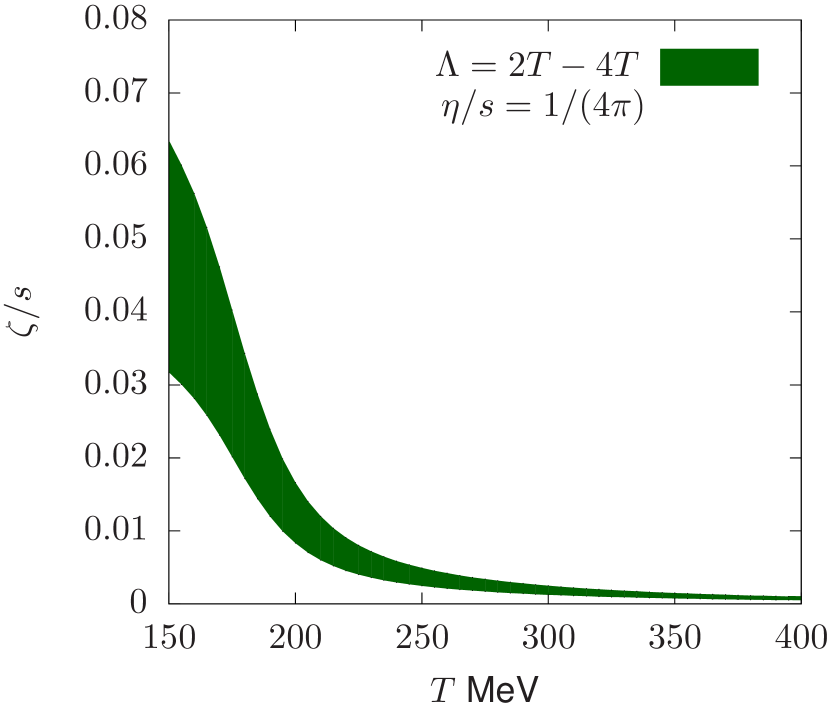
Figure 1: A fluctuation-induced bulk viscosity bound as a function of temperature, Eq. (1), for lattice parametrization of the QCD equation of state and shear viscosity over entropy $\eta/s=1/(4\pi)$ Borsanyi et al. (2016). The UV bound of hydrodynamic fluctuations $\Lambda$ is varied between $2T$ and $4T$.

Because of the small deviation from scale symmetry at high temperatures the bulk viscosity renormalization is vanishing small for $T\gg T_{c}$. However, the degree of nonconformality $(c_{s}^{2}-\frac{1}{3})^{2}$ peaks around the pseudocritical temperature where the bulk viscosity reaches $\zeta/s\sim 0.03-0.06$ at $T_{c}\sim 150\,\text{MeV}$.

The logic of the estimate in Fig. 1 is the following. The physical bulk viscosity $\zeta(T)$ (which is independent of $\Lambda$) arises from two contributions: the fluctuations above $\Lambda$, which at weak coupling are dominated by single-particle excitations, and the fluctuations below $\Lambda$, which are described by hydrodynamics. We have only included the hydrodynamic fluctuations here, and thus we expect the physical bulk viscosity to be larger than the estimate shown in Fig. 1.

The organization of this paper is as follows. In Sec. II, we derive the kinetic equations for hydrodynamic fluctuations for an isotropically expanding nonconformal fluid. Then in Sec. III, we compute the fluctuation contributions to the energy-momentum tensor, and discuss the subtle temperature shift. After the temperature shift, we renormalize the energy density, the pressure, and the bulk viscosity, and find the finite long-time tails for the weak isotropic expansion. The summary of the paper is given in Sec. IV. Finally, in Appendix A we repeat the computation of the temperature shift and the renormalization of hydrodynamic fields for Bjorken expansion. In Appendix B, we give a diagrammatic derivation for the bulk viscosity renormalization, which is consistent with our results by the hydrokinetic theory.

II Kinetic equations for hydrodynamic fluctuations

In this section we apply the formalism developed in Ref. Akamatsu et al. (2017) to a nonconformal fluid under isotropic expansion (or compression). We will follow the same procedure to derive the relaxation type equations for the two-point correlation functions under the presence of background perturbations.

The governing equations for nonconformal hydrodynamics with noise are given by Landau and Lifshitz (1980); Lifshitz and Pitaevskii (1980); [forarecentreview:]Kovtun:2012rj

$$d_{\mu}T^{\mu\nu} =0,\quad T^{\mu\nu}=T^{\mu\nu}_{\text{ideal}}+T^{\mu\nu}_{\text{visc.}}+S^{\mu\nu},$$ (2a)

$$T^{\mu\nu}_{\rm ideal} =(e+p)u^{\mu}u^{\nu}+pg^{\mu\nu},$$ (2b)

$$T^{\mu\nu}_{\rm visc.} =-\eta\sigma^{\mu\nu}-\zeta\Delta^{\mu\nu}\Delta^{\alpha\beta}d_{\alpha}u_{\beta},$$ (2c)

$$\sigma^{\mu\nu} =\Delta^{\mu\rho}\Delta^{\nu\sigma}(d_{\rho}u_{\sigma}+d_{\sigma}u_{\rho}-\frac{2}{3}g_{\rho\sigma}d_{\gamma}u^{\gamma}),$$ (2d)

$$\Delta^{\mu\nu} =g^{\mu\nu}+u^{\mu}u^{\nu},$$ (2e)

where $d_{\mu}$ denotes a covariant derivative using the “mostly-plus” metric convention. Below we notate the divergence of the flow velocity as $\nabla\cdot u\equiv d_{\mu}u^{\mu}$. The variance of the stochastic noise is determined by the fluctuation-dissipation theorem:

$$\langle S^{\mu\nu}(x_{1})S^{\alpha\beta}(x_{2})\rangle$$

$$=2T\left[\begin{aligned} &\eta\left(\Delta^{\mu\alpha}\Delta^{\nu\beta}+\Delta^{\mu\beta}\Delta^{\nu\alpha}\right)\\ &+\left(\zeta-\frac{2}{3}\eta\right)\Delta^{\mu\nu}\Delta^{\alpha\beta}\end{aligned}\right]\frac{\delta(x_{1}-x_{2})}{\sqrt{-\det g_{\mu\nu}}}.$$ (3)

Differently from the conformal case, both shear $\eta$ and bulk $\zeta$ viscosities are now present in the equation of motion and noise correlator.

II.1 Background fluid

Dynamics of hydrodynamic fluctuations on a background fluid in a weak isotropic expansion (or compression) is conveniently studied in the reference frame of the fluid. In the comoving frame for the isotropic expansion, the metric is time dependent,

$$ds^{2}=-dt^{2}+(1+h(t))d\vec{x}^{2},\ \ \ (|h(t)|\ll 1)$$ (4)

and the background fluid satisfies

$$0=\dot{e}_{0}(t)+\frac{3\dot{h}}{2}[e_{0}(t)+p_{0}(t)]+\mathcal{O}(h^{2}).$$ (5)

The second term on the right-hand side represents the change of energy density from the expansion and the associated work done by the pressure. Throughout this paper, $X_{0}$ denotes a quantity $X$ of the background fluid in a perturbed metric ($h\neq 0$). As discussed previously Akamatsu et al. (2017), $e_{0}(t)$ and $p_{0}(t)$ denote the background energy density and pressure from modes with wavenumbers greater than a cut-off $\Lambda$. In Sec. III.2 we detail how $e_{0}$ and $p_{0}$ are related to the lattice equation of state.

Solving perturbatively in $h$, the energy density $e_{0}(t)$ for the background fluid evolves as

$$e_{0}(t)=\bar{e}_{0}-\frac{3h(t)}{2}(\bar{e}_{0}+\bar{p}_{0})+\mathcal{O}(h^{2}),$$ (6)

where $\bar{e}_{0}$ denotes the energy density of the background fluid in an unperturbed state ($h=0$). Again, throughout this paper $\bar{X}_{0}$ denotes a quantity $X$ of the background fluid in an unperturbed state ($h=0$).

II.2 Evolution of hydrodynamic fluctuations

For the expanding background described by Eq. (6), the hydrodynamic fluctuations excited by thermal noise $\delta e(t,{\bm{x}})\equiv e(t,{\bm{x}})-e_{0}(t)$ and $\vec{g}\equiv(e_{0}(t)+p_{0}(t))\vec{v}(t,{\bm{x}})$ evolve according to the following equations in ${\bm{k}}$ space:

$$0 =\partial_{t}\delta e+ik^{i}g_{i}+\frac{3\dot{h}}{2}(1+c_{s0}^{2})\delta e,$$ (7a)

$$0 =\partial_{t}g_{i}+ic_{s0}^{2}k_{i}\delta e+\frac{3\dot{h}}{2}g_{i}$$

$$\quad+\gamma_{\eta 0}(k^{l}k_{l}\delta_{i}^{j}-k_{i}k^{j})g_{j}+\gamma_{\zeta 0}k_{i}k^{j}g_{j}+\xi_{i},$$ (7b)

with noise correlation given by

$$\langle\xi_{i}(t,\bm{k})\xi_{j}(t^{\prime},-\bm{k}^{\prime})\rangle =\frac{2T_{0}(e_{0}+p_{0})}{\sqrt{-\text{det}\,g_{\mu\nu}}}(2\pi)^{3}\delta(\bm{k}-\bm{k}^{\prime})\delta(t-t^{\prime})$$

$$\quad\times\left[\gamma_{\eta 0}(k^{l}k_{l}g_{ij}-k_{i}k_{j})+\gamma_{\zeta 0}k_{i}k_{j}\right].$$ (8)

Here $\gamma_{\eta}\equiv\eta/(e+p)$ and $\gamma_{\zeta}\equiv(\zeta+\frac{4}{3}\eta)/(e+p)$ are kinematic viscosities. Analysis becomes simpler by utilizing a vielbein formalism. We introduce new variables

$$G_{\hat{i}} \equiv\left(1+\frac{1}{2}h(t)\right)g^{i},$$ (9a)

$$K_{\hat{i}} \equiv\left(1-\frac{1}{2}h(t)\right)k_{i},$$ (9b)

$$\Xi_{\hat{i}} \equiv\left(1+\frac{1}{2}h(t)\right)\xi^{i},$$ (9c)

which give $G_{\hat{i}}G_{\hat{i}}=g_{i}g^{i}$, $K_{\hat{i}}K_{\hat{i}}=k_{i}k^{i}$, and $G_{\hat{i}}K_{\hat{i}}=g^{i}k_{i}=g_{i}k^{i}$. We define a four-component vector $\phi_{a}\equiv(c_{s0}\delta e,\vec{G})$ of hydrodynamic fluctuations. The equation of motion for $\phi_{a}$ is

$$-\dot{\phi}_{a}(t,\bm{k}) =i\mathcal{L}_{ab}\phi_{b}+\mathcal{D}_{ab}\phi_{b}+\Xi_{a}+\mathcal{P}_{ab}\phi_{b},$$ (10a)

$$\mathcal{L}=\left(\begin{array}[]{cc}0&c_{s0}\vec{K}\\ c_{s0}\vec{K}&0\end{array}\right),$$ (10d)

$$\mathcal{D}=\left(\begin{array}[]{cc}0&0\\ 0&\gamma_{\eta 0}\left(K^{2}\delta_{\hat{i}\hat{j}}-K_{\hat{i}}K_{\hat{j}}\right)+\gamma_{\zeta 0}K_{\hat{i}}K_{\hat{j}}\end{array}\right),$$ (10g)

$$\mathcal{P}=\dot{h}\left(\begin{array}[]{cccc}\frac{3}{2}\left(1+\bar{c}_{s0}^{2}+\frac{\bar{T}_{0}}{2}\frac{d\bar{c}_{s0}^{2}}{d\bar{T}_{0}}\right)&&&\\ &2&&\\ &&2&\\ &&&2\end{array}\right),$$ (10l)

with noise correlation given by

$$\langle\Xi_{a}(t,\bm{k})\Xi_{b}(t^{\prime},-\bm{k}^{\prime})\rangle$$

$$\quad=\frac{2T_{0}(e_{0}+p_{0})}{\sqrt{-\text{det}\,g_{\mu\nu}}}\mathcal{D}_{ab}(2\pi)^{3}\delta(\bm{k}-\bm{k}^{\prime})\delta(t-t^{\prime}).$$ (11)

The matrices $\mathcal{L}$ and $\mathcal{D}$ originate from ideal and viscous parts of the hydrodynamic equations respectively, while $\mathcal{P}$ arises from the remaining interactions between the fluctuations and the background fluid. Note that the term $\propto\frac{\bar{T}_{0}}{2}\frac{d\bar{c}_{s0}^{2}}{dT_{0}}$ in $\mathcal{P}$ derives from the time dependence of $c_{s0}(T_{0}(t))\delta e$ in $\phi_{1}$. In the kinetic regime, $\mathcal{L}$ drives the evolution of $\phi_{a}$ so that it will be more convenient to analyze Eq. (10a) in terms of eigenmodes of $\mathcal{L}$:

$$(e_{\pm})_{a}=\frac{1}{\sqrt{2}}\begin{pmatrix}1\\ \pm\hat{K}\end{pmatrix},\quad(e_{T_{1}})_{a}=\begin{pmatrix}0\\ \vec{T}_{1}\\ \end{pmatrix},\quad(e_{T_{2}})_{a}=\begin{pmatrix}0\\ \vec{T}_{2}\\ \end{pmatrix}.$$

Here $\hat{K}\equiv\vec{K}/|K|$, $\vec{T}_{1}$, and $\vec{T}_{2}$ form an orthonormal basis. The subscripts $+,-$ stand for the two sound modes and $T_{1},T_{2}$ for the two transverse diffusive modes. The corresponding eigenvalues are $\lambda_{\pm}=\pm c_{s}K$ and $\lambda_{T_{1},T_{2}}=0$.

II.3 Kinetic equations for hydrodynamic fluctuations

The two-point correlation functions of $\phi_{A}\equiv\phi_{a}\left(e_{A}\right)_{a}$ with $A=+,-,T_{1},T_{2}$ are defined as

$$\left\langle\phi_{A}(t,\bm{k})\phi_{B}(t,-\bm{k}^{\prime})\right\rangle\equiv N_{AB}(t,\bm{k})(2\pi)^{3}\delta(\bm{k}-\bm{k}^{\prime}).$$ (13)

We will determine the equations of motion for $N_{AB}(t,{\bm{k}})$ using the formalism of Ref. Akamatsu et al. (2017). In the rotating wave approximation, the off-diagonal part of the density matrix $N_{AB}$ can be neglected because of its rapid phase rotation, while the diagonal part evolves according to

$$\dot{N}_{AA}=-2\mathcal{D}_{AA}\left[N_{AA}-\frac{T_{0}(e_{0}+p_{0})}{\sqrt{-\det g_{\mu\nu}}}\right]+2\mathcal{P}_{AA}N_{AA},$$

where we have defined $\mathcal{D}_{AA}\equiv(e_{A})_{a}\mathcal{D}_{ab}(e_{A})_{b}$ and similarly $\mathcal{P}_{AA}$. The isotropic system does not distinguish the two transverse modes $T_{1}$ and $T_{2}$, and thus we only have two independent kinetic equations: one for the sound modes ($L=++,--$), and one for the transverse modes ($T=T_{1}T_{1},T_{2}T_{2}$). Using the matrices and eigenvectors of the previous section, Eq. (II.3) evaluates to

$$\dot{N}_{L} =-\gamma_{\zeta 0}K^{2}\left[N_{L}-\frac{T_{0}(e_{0}+p_{0})}{\sqrt{-\det g_{\mu\nu}}}\right]$$

$$\quad-\frac{\dot{h}}{2}\left(3\bar{c}_{s0}^{2}+\frac{3\bar{T}_{0}}{2}\frac{d\bar{c}_{s0}^{2}}{d\bar{T}_{0}}+7\right)N_{L},$$ (15a)

$$\dot{N}_{T} =-2\gamma_{\eta 0}K^{2}\left[N_{T}-\frac{T_{0}(e_{0}+p_{0})}{\sqrt{-\det g_{\mu\nu}}}\right]-4\dot{h}N_{T}.$$ (15b)

The kinetic equations (15) and (15b) describe how the distribution of fluctuations $\phi_{A}$ evolves on the isotropically expanding background. Perturbative solutions of the kinetic equations for $|h|\ll 1$ take the form,

$$N_{L/T}(t,\bm{k}) =N_{\rm eq}(t)+\delta N_{L/T}(t,\bm{k})+\mathcal{O}(h^{2}),$$ (16)

where the equilibrium contribution is

$$N_{\rm eq}(t) =\frac{T_{0}(e_{0}+p_{0})}{\sqrt{-\det g_{\mu\nu}}}$$

$$\simeq\left[1-(3+3\bar{c}_{s0}^{2})h(t)\right]\bar{T}_{0}(\bar{e}_{0}+\bar{p}_{0}),$$ (17)

and the non-equilibrium correction $\delta N_{L/T}$ is

$$\delta N_{L}(\omega,\bm{k}) =\frac{\frac{1}{2}i\omega h(\omega)}{-i\omega+\bar{\gamma}_{\zeta 0}K^{2}}\bar{C}_{\zeta 0}\bar{T}_{0}(\bar{e}_{0}+\bar{p}_{0}),$$ (18a)

$$\delta N_{T}(\omega,\bm{k}) =\frac{i\omega h(\omega)}{-i\omega+2\bar{\gamma}_{\eta 0}K^{2}}\bar{C}_{\eta 0}\bar{T}_{0}(\bar{e}_{0}+\bar{p}_{0}).$$ (18b)

Here and below we have defined

$$C_{\zeta}(T) \equiv 1+\frac{3T}{2}\frac{dc_{s}^{2}}{dT}-3c_{s}^{2},$$ (19a)

$$C_{\eta}(T) \equiv 1-3c_{s}^{2}.$$ (19b)

Note that when the background fluid is scale invariant $e_{0}=3p_{0}$, the corrections $\delta N_{L/T}$ vanish. Therefore in conformal case, the isotropic expansion or compression does not drive the hydrodynamic fluctuations from the equilibrium distribution $N_{\text{eq}}(t)$ given by Eq. (II.3).

For $k\sim k_{*}$ the distribution of fluctuations in Eq. (18) is not well characterized by the time derivatives of $h(t)$. However, at large $k$ by the distribution approaches equilibrium with calculable first derivative corrections:

$$\delta N_{L}(t,\bm{k}) \simeq-\frac{3\bar{C}_{\zeta 0}\bar{T}_{0}(\bar{e}_{0}+\bar{p}_{0})}{\bar{\gamma}_{\zeta 0}K^{2}}\,\nabla\cdot u,$$ (20a)

$$\delta N_{T}(t,\bm{k}) \simeq-\frac{3\bar{C}_{\eta 0}\bar{T}_{0}(\bar{e}_{0}+\bar{p}_{0})}{2\bar{\gamma}_{\eta 0}K^{2}}\,\nabla\cdot u.$$ (20b)

It is these corrections $\propto\nabla\cdot u/K^{2}$ which are responsible for the renormalization of the bulk viscosity and the temperature shift described in Sect. III.

III Energy-momentum tensor with nonlinear fluctuations

In this section we compute the nonlinear contributions of hydrodynamic fluctuations to the statistically averaged energy momentum tensor $\left<T^{\mu\nu}\right>$. The main difference from the conformal case Akamatsu et al. (2017) is additional contributions to the averaged energy density $\left<T^{tt}\right>$, which are absorbed by a shift in the background temperature $T_{0}(t,\Lambda)$.

III.1 Averaged energy-momentum tensor

The averaged stress tensor consists of contributions from the background fluid and from the two-point functions of the hydrodynamic fluctuations:

$$\langle T^{ij}\rangle =\left[1-h(t)\right]p_{0}\delta^{ij}-\frac{3}{2}\dot{h}(t)\zeta_{0}\delta^{ij}+T^{ij}_{\rm fluct},$$ (21a)

$$T^{ij}_{\rm fluct} \simeq\frac{1-h(t)}{e_{0}+p_{0}}\left[\begin{aligned} &\langle G_{\hat{i}}(t,\bm{x})G_{\hat{j}}(t,\bm{x})\rangle\\ &+\delta^{ij}\frac{T_{0}}{2}\frac{dc_{s0}^{2}}{dT_{0}}\langle(c_{s0}\delta e(t,\bm{x}))^{2}\rangle\end{aligned}\right].$$ (21b)

The energy density fluctuations $\propto\langle(c_{s0}\delta e(t,\bm{x}))^{2}\rangle$ originate from the second-order derivative $\frac{d^{2}p_{0}}{de_{0}^{2}}$, which is finite for a nonconformal equation of state. The trace of the stress tensor from the fluctuations is determined by the two-point functions $N_{L/T}$:

$$T^{ii}_{\rm fluct} =\frac{1-h(t)}{e_{0}+p_{0}}\int\frac{d^{3}k}{(2\pi)^{3}}$$ (22)

$$\quad\times\left[\left(1+\frac{3T_{0}}{2}\frac{dc_{s0}^{2}}{dT_{0}}\right)N_{L}(t,\bm{k})+2N_{T}(t,\bm{k})\right].$$

This integral is divergent and is regularized by introducing a cut off $\Lambda$ for $K$ (not $k$). Substituting the solution (16), we write the fluctuating contribution as a sum of two terms,

$$T^{ii}_{\rm fluct}(t,\Lambda)=T^{ii}_{N_{\rm eq}}(t;\Lambda)+T^{ii}_{\delta N}(t;\Lambda).$$ (23)

The first term arises from equilibrium fluctuations $N_{\rm eq}(t)$ (Eq. (II.3))

$$T^{ii}_{N_{\rm eq}}(t;\Lambda)\equiv[1-h(t)]\left(1+\frac{T_{0}}{2}\frac{dc_{s0}^{2}}{dT_{0}}\right)\frac{T_{0}\Lambda^{3}}{2\pi^{2}},$$ (24)

while the second term arises from the nonequilibrium distribution functions, $\delta N_{L/T}$ in Eq. (18). In frequency space this nonequilibrium contribution reads

$$T^{ii}_{\delta N}(\omega;\Lambda)\equiv \frac{h(\omega)\bar{T}_{0}}{4\pi^{2}}\left(1+\frac{3\bar{T}_{0}}{2}\frac{d\bar{c}_{s0}^{2}}{d\bar{T}_{0}}\right)\bar{C}_{\zeta 0}f(\omega,\bar{\gamma}_{\zeta 0},\Lambda)$$

$$\quad+\frac{h(\omega)\bar{T}_{0}}{\pi^{2}}\bar{C}_{\eta 0}f(\omega,2\bar{\gamma}_{\eta 0},\Lambda).$$ (25)

Here we have defined a function,

$$f(\omega,\gamma,\Lambda) \equiv\int_{0}^{\Lambda\to\infty}p^{2}dp\frac{i\omega}{-i\omega+\gamma p^{2}}$$ (26)

$$=\frac{i\omega}{\gamma}\Lambda-\left(\frac{|\omega|}{\gamma}\right)^{3/2}\frac{\pi}{2\sqrt{2}}(1+i{\rm sgn}(\omega)).$$

Next, we calculate the averaged energy density in a similar manner. It also consists of contributions from the background fluid and from the two-point functions of the fluctuations:

$$\langle T^{tt}\rangle =e_{0}+T^{tt}_{\rm fluct},$$ (27a)

$$T^{tt}_{\rm fluct} =\frac{\langle\vec{G}^{2}\rangle}{e_{0}+p_{0}}$$ (27b)

$$=\frac{1}{e_{0}+p_{0}}\int\frac{d^{3}k}{(2\pi)^{3}}\left[N_{L}(t,\bm{k})+2N_{T}(t,\bm{k})\right],$$

The contribution from the fluctuations is again divergent and we regularize with the same cut-off $\Lambda$ on $K$. Substituting the perturbative solutions (16), we find

$$T^{tt}_{\rm fluct}(t;\Lambda)= T^{tt}_{N_{\rm eq}}(t;\Lambda)+T^{tt}_{\delta N}(t;\Lambda),$$ (28)

where the first term arises from the equilibrium distribution $N_{\rm eq}$ (Eq. (II.3))

$$T^{tt}_{N_{\rm eq}}(t;\Lambda)\equiv\frac{T_{0}\Lambda^{3}}{2\pi^{2}},$$ (29)

while the second term (in frequency space) arises from $\delta N_{L/T}$,

$$T^{tt}_{\delta N}(\omega;\Lambda)\equiv \frac{h(\omega)\bar{T}_{0}}{4\pi^{2}}\bar{C}_{\zeta 0}f(\omega,\bar{\gamma}_{\zeta 0},\Lambda)\,$$

$$\quad+\frac{h(\omega)\bar{T}_{0}}{\pi^{2}}\bar{C}_{\eta 0}f(\omega,2\bar{\gamma}_{\eta 0},\Lambda).$$ (30)

As will be described in the next section, the divergences in $T^{ii}_{\text{fluct}}$ and $T^{tt}_{\text{fluct}}$ are absorbed by renormalizing the background fields, e.g., $p_{0}$ and $\zeta_{0}$. This renormalization procedure requires a clearer understanding how these bare parameters are defined, and how they depend on the cut-off $\Lambda$.

III.2 Temperature shift

The bare parameters $e_{0},p_{0},T_{0},\zeta_{0},\ldots$ are determined by modes (such as particlelike excitations) with wave numbers above the cut-off, $k>\Lambda$, which are not explicitly propagated by the statistical hydrodynamic system. The goal of this section is to carefully explain how these parameters are defined and related to the physical equation of state $e(T),\,p(T)$ (from lattice QCD) and the cut-off $\Lambda$.

First consider the density matrix for nonhydrodynamic modes with wave numbers above the cut-off $k>\Lambda$. When the system is driven slightly out of equilibrium by the periodic compression and expansion, the density matrix for these modes $\rho(\Lambda)$ can be decomposed as an equilibrium density matrix $\rho_{\rm eq}(T_{0};\Lambda)$ and a nonequilibrium correction which is well characterized by a single gradient $\delta\rho_{\rm neq}(\Lambda)\propto\nabla\cdot u$,

$$\rho(\Lambda)=\rho_{\rm eq}(T_{0};\Lambda)+\delta\rho_{\rm neq}(\Lambda)\,.$$ (31)

The temperature parameter $T_{0}$ (which will depend on time and $\Lambda$) is chosen so that the average energy density above the cut-off $e_{0}(t,\Lambda)\equiv\left\langle T^{tt}(t)\right\rangle_{k>\Lambda}$ equals the energy from the equilibrium density matrix $\rho_{\rm eq}(T_{0};\Lambda)$ alone

$$e_{0}(t,\Lambda)\equiv\left\langle T^{tt}(t)\right\rangle_{k>\Lambda}=e_{\rm eq,0}(T_{0}(t;\Lambda);\Lambda)\,,$$ (32)

i.e., $T_{0}(t;\Lambda)$ is adjusted so that the energy moment associated with $\delta\rho_{\rm neq}(\Lambda)$ is zero $\delta e_{\rm neq}(t;\Lambda)=0$. (Otherwise the rhs of Eq. (32) would have a correction proportional to $\nabla\cdot u$). Because of the constraint in Eq. (32) we can drop the “eq” label below, i.e.,

$$e_{0}(t,\Lambda)=e_{\rm eq,0}(T_{0}(t;\Lambda);\Lambda)=e_{0}(T_{0}(t;\Lambda);\Lambda).$$ (33)

In kinetic theory a similar constraint is imposed by requiring that the viscous correction to the distribution function $\delta f_{\rm bulk}({\bf p})$ does not change the energy in the system Arnold et al. (2006); Moore and Saremi (2008). Once this prescription for $T_{0}(t;\Lambda)$ is adopted, the stress computed with the density matrix $\rho(\Lambda)$ is given by

$$\left\langle T^{ij}\right\rangle_{k>\Lambda}=(1-h)\,p_{0}(T_{0};\Lambda)\,\delta^{ij}-\zeta_{0}(T_{0};\Lambda)\,\nabla\cdot u\,\delta^{ij}\,,$$ (34)

where the partial pressure $p_{0}(T_{0};\Lambda)$ from modes above $\Lambda$ is determined by the equilibrium density matrix, $\rho_{\rm eq}(T_{0};\Lambda)$, while the bulk term comes from the viscous correction, $\delta\rho_{\rm neq}(\Lambda)$. This is the parametrization of the stress tensor (for $k>\Lambda$) that was used in Eq. (2). The spatial stress tensor determines the bulk viscous correction $\zeta_{0}\nabla\cdot u$ only after the parameter $T_{0}(t;\Lambda)$ is defined according to the Landau constraint in Eq. (32) Arnold et al. (2006); Moore and Saremi (2008).

Later in this section we will define a temperature $T(t)$ by imposing the Landau constraint on the whole system (including the energy of hydrodynamic fluctuations below the cut-off), and this will lead to a difference between $T_{0}(t;\Lambda)$ and the cutoff independent temperature $T(t)$.

Now we will relate the partial energy density and pressure, $e_{0}(T_{0};\Lambda)$ and $p_{0}(T_{0};\Lambda)$, to the equilibrium energy density and pressure, $e(T_{0})$ and $p(T_{0})$, as measured by lattice QCD. Indeed, $e_{0}$ and $p_{0}$ are cut-off dependent quantities and are determined by an equilibrium density matrix $\rho_{\rm eq}(T_{0};\Lambda)$ which excludes equilibrium hydrodynamic fluctuations below the scale $\Lambda$. The contribution of such equilibrium hydrodynamic fluctuations to the energy density and pressure are given by Eq. (29) and Eq. (24), respectively, and thus the physical energy density and pressure are:

$$e(T_{0})= e_{0}(T_{0};\Lambda)+\frac{T_{0}\Lambda^{3}}{2\pi^{2}}\,,$$ (35a)

$$p(T_{0})= p_{0}(T_{0};\Lambda)+\left(1+\frac{T_{0}}{2}\frac{dc_{s}^{2}}{dT_{0}}\right)\frac{T_{0}\Lambda^{3}}{6\pi^{2}}\,.$$ (35b)

At a practical level these equations serve to define the $e_{0}$ and $p_{0}$ parameters that should be used in a stochastic hydrocode with a given cut-off $\Lambda$ and physical equation of state $e(T_{0}),\,p(T_{0})$.

As discussed above, the temperature $T(t)$ for the complete system (background+fluctuations) is adjusted so that the energy density calculated from the lattice equation of state $e(T(t))$ matches the energy of the partially equilibrated system $\left\langle T^{tt}(t)\right\rangle$,

$$\left\langle T^{tt}(t)\right\rangle=e(T(t))\,.$$ (36)

After imposing this constraint, the time-dependent stress $\left\langle T^{ii}(t)\right\rangle$ of the driven system will deviate from its equilibrium expectation, $3\,p(T(t))\,(1-h(t))$, and these deviations are described (up to long-time tails) by the bulk viscosity. Combining Eqs. (27a), (28), (29), and (35a), the energy of the background+fluctuations is

$$e(T(t)) =e(T_{0}(t;\Lambda))+T^{tt}_{\delta N}(t;\Lambda),$$ (37)

where $T^{tt}_{\delta N}(t;\Lambda)$ was defined in Eq. (III.1). Thus, the temperature for the whole system $T(t)$ (which is independent of the cut-off) is related to the temperature parameter of the subsystem $T_{0}(t;\Lambda)$ by a small shift $\Delta T$

$$T_{0}(t;\Lambda)=T(t)+\Delta T(t;\Lambda)\,,$$ (38)

so that Eq. (37) is satisfied. The temperature shift is given in frequency space by

$$-\frac{de}{dT}\Delta T(\omega;\Lambda) =\frac{h(\omega)\bar{T}}{4\pi^{2}}\bar{C}_{\zeta 0}f(\omega,\bar{\gamma}_{\zeta 0},\Lambda)$$ (39)

$$\quad+\frac{h(\omega)\bar{T}}{\pi^{2}}\bar{C}_{\eta 0}f(\omega,2\bar{\gamma}_{\eta 0},\Lambda).$$

and clearly depends on the cutoff because the $T_{0}(t;\Lambda)$ was defined with respect to a specific subsystem labeled by $\Lambda$. The temperature shift in the time domain takes the form

$$-\frac{de}{dT}\Delta T(t;\Lambda)=-\frac{\bar{T}\Lambda}{6\pi^{2}}\left[\frac{\bar{C}_{\zeta 0}}{\bar{\gamma}_{\zeta 0}}+4\frac{\bar{C}_{\eta 0}}{2\bar{\gamma}_{\eta 0}}\right]\nabla\cdot u\\ +{\rm finite}\,,$$ (40)

where $\nabla\cdot u=\tfrac{3}{2}\dot{h}$ for this example. The divergent piece of the temperature shift is universal, but the finite corrections are not. This is verified by explicit calculation of the temperature shift for the Bjorken background in Appendix A. From practical perspective, Eqs. (38) and (40) define how $T_{0}$ must be chosen for a stochastic hydro code (with a specified cut-off $\Lambda$) to reproduce the correct physical bulk viscosity for long wavelength hydrodynamic modes and a physical equation of state. This is detailed in the next section.

III.3 Renormalized background and long-time tails

Once the temperature shift $\Delta T(t;\Lambda)$ is obtained, the remaining divergences in $T^{ii}_{\rm fluct}$ can be absorbed by pressure and bulk viscosity renormalization. Using Eqs. (21a), (23), (24), and (35b), the statistically averaged spatial stress tensor trace reads

$$\langle T^{ii}\rangle(t)=3\left[1-h(t)\right]p(T_{0}(t;\Lambda))\\ -\frac{9}{2}\dot{h}(t)\zeta_{0}+T^{ii}_{\delta N}(t;\Lambda).$$ (41)

where $T^{ii}_{\delta N}$ is given in Eq. (III.1).

Now we will shift the temperature parameter $T_{0}$ in the pressure to the physical temperature $T(t)$ determined by Landau matching (37), $p(T_{0})=p(T)+p^{\prime}(T)\Delta T$. The fluctuation contribution $T^{ii}_{\delta N}(t;\Lambda)$ and the temperature parameter $\Delta T(t;\Lambda)$ both diverge as $-i\omega h(\omega)\Lambda$. These two terms gracefully combine to produce a positive definite renormalization of bulk viscosity $\zeta_{0}$ in the term $-\frac{9}{2}\dot{h}(t)\zeta$,

$$\zeta(T)=\zeta_{0}(T;\Lambda)+\frac{T\Lambda}{18\pi^{2}}\left[\frac{C_{\zeta 0}^{2}}{\gamma_{\zeta 0}}+4\frac{C_{\eta 0}^{2}}{2\gamma_{\eta 0}}\right]\,.$$ (42)

In this step the coefficients in front of the linear divergences in $\Delta T$ and $T^{ii}_{\delta N}$ have neatly come together to complete the squares of $C_{\zeta 0}$ and $C_{\eta 0}$ defined by Eq. (19). Thus the renormalization of the bulk viscosity is positive and only necessary in a system with broken scale symmetry. We have confirmed that the bulk viscosity renormalization is universal by computing it for a Bjorken expanding background (see Appendix A).

Once all divergences are absorbed by renormalization, the stress tensor becomes finite and cut-off independent. In the presence of background expansion, there are remaining finite corrections from the fluctuations in $T^{ii}_{\delta N}$. The total stress tensor is

$$\langle T^{ii}\rangle(t) =3\left[1-h(t)\right]p(T(t))-\frac{9}{2}\dot{h}(t)\zeta(T(t))$$

$$\quad-\int\frac{d\omega}{2\pi}e^{-i\omega t}h(\omega)|\omega|^{3/2}\frac{\pi}{2\sqrt{2}}(1+i{\rm sgn}(\omega))$$

$$\quad\quad\times\frac{\bar{T}}{4\pi^{2}}\left[\bar{C}_{\zeta 0}^{2}\left(\frac{1}{\bar{\gamma}_{\zeta 0}}\right)^{3/2}+4\bar{C}_{\eta 0}^{2}\left(\frac{1}{2\bar{\gamma}_{\eta 0}}\right)^{3/2}\right],$$

and has a term with $|\omega|^{3/2}$, which cannot be expressed by local time derivatives. This term is not analytic at $\omega=0$ and derives from the out-of-equilibrium fluctuations in the kinetic regime $k\sim k_{*}$.

With $\langle T^{tt}\rangle$ and $\langle T^{ii}\rangle$ known, we can write down the hydrodynamic equations for statistically averaged hydrodynamics with noise

$$0=\frac{d}{dt}\langle T^{tt}\rangle+\frac{3}{2}\dot{h}\langle T^{tt}\rangle+\frac{1}{2}\dot{h}\langle T^{ii}\rangle.$$ (43)

Because the nonanalytic term in $\langle T^{ii}\rangle$ is of $\mathcal{O}(h)$, the rest frame energy density $e(t)$ evolves according to

$$0=\dot{e}(t)+\frac{3\dot{h}}{2}\left[e(t)+p(t)\right],$$ (44)

and we obtain the solution:

$$e(t)=\bar{e}-\frac{3h(t)}{2}(\bar{e}+\bar{p}),$$ (45)

which will be used to calculate the response function in the next section.

III.4 Response function in the bulk channel

The nonanalytic behavior in $\omega$ is also present in the response function in the bulk channel. In the frequency space, the linear response of stress tensor to the external gravitational field $h(\omega)$ is given by

$$\langle T^{ii}\rangle(\omega)=G_{R}^{ii,jj}(\omega,\bm{k}=\bm{0})\frac{1}{2}h(\omega).$$ (46)

The response function $G_{R}^{ii,jj}$ is defined by

$$G_{R}^{ii,jj}(t,\bm{x}) \equiv i\theta(t)\left\langle\left[\hat{T}^{ii}(t,\bm{x}),\hat{T}^{jj}(0,\bm{0})\right]\right\rangle,$$ (47a)

$$G_{R}^{ii,jj}(\omega,\bm{k}) =\int d^{4}x\,G_{R}^{ii,jj}(t,\bm{x})e^{i\omega t-i\bm{k}\cdot\bm{x}}.$$ (47b)

Then from our results, the response function $G_{R}^{ii,jj}(\omega)\equiv G_{R}^{ii,jj}(\omega,\bm{k}=\bm{0})$ is obtained as

$$G_{R}^{ii,jj}(\omega)=\frac{\delta}{\delta h(\omega)}\left[2\langle T^{ii}\rangle(\omega)\right]\Big{|}_{h=0}$$

$$=-6\left(\bar{p}+\frac{3}{2}\bar{c}_{s}^{2}(\bar{e}+\bar{p})\right)+9i\omega\bar{\zeta}-\frac{1+i{\rm sgn}(\omega)}{4\sqrt{2}\pi}|\omega|^{3/2}\bar{T}$$

$$\quad\times\left[\bar{C}_{\zeta}^{2}\left(\frac{1}{\bar{\gamma}_{\zeta}}\right)^{3/2}+4\bar{C}_{\eta}^{2}\left(\frac{1}{2\bar{\gamma}_{\eta}}\right)^{3/2}\right],$$ (48)

and the spectral function as

$$\rho^{ii,jj}(\omega)=2{\rm Im}\,G_{R}^{ii,jj}(\omega)$$ (49)

$$=18\omega\bar{\zeta}-\frac{\omega|\omega|^{1/2}\bar{T}}{2\sqrt{2}\pi}\left[\bar{C}_{\zeta}^{2}\left(\frac{1}{\bar{\gamma}_{\zeta}}\right)^{3/2}+4\bar{C}_{\eta}^{2}\left(\frac{1}{2\bar{\gamma}_{\eta}}\right)^{3/2}\right].$$

This spectral function is consistent with a previous diagrammatic computation of the symmetrized correlation function $C^{ii,jj}$ (see the appendix of Ref. Kovtun and Yaffe (2003)) using the fluctuation-dissipation relation:

$$\rho^{ii,jj}(\omega) =\frac{\omega}{T}C^{ii,jj}(\omega,\bm{k}=\bm{0}),$$ (50a)

$$C^{ii,jj}(t,\bm{x}) \equiv\frac{1}{2}\left\langle\left\{\hat{T}^{ii}(t,\bm{x}),\hat{T}^{jj}(0,\bm{0})\right\}\right\rangle_{\rm conn}.$$ (50b)

We also computed $G_{R}^{ii,jj}(\omega)$ diagrammatically in Appendix B and found identical results to Eqs. (48) and (42) up to a contact term.

IV Summary

In this paper we applied the kinetic theory of hydrodynamic fluctuations developed in Ref. Akamatsu et al. (2017) to a relativistic nonconformal fluid. We calculated the contribution of out-of-equilibrium hydrodynamic fluctuations to the energy momentum tensor, which renormalize the background hydrodynamic fields and the bulk viscosity $\zeta$. The bulk viscosity renormalization is proportional to the scaling symmetry breaking in the equation of state and can be used to estimate the minimal bulk viscosity value in a hot QCD medium.

In the main body of the paper, we considered a nonconformal charge-neutral fluid, which is driven out of equilibrium by a weak isotropic expansion (or compression). Analogous calculations for a Bjorken expanding system is summarized in the appendix. The relaxation of hydrodynamic fluctuations to equilibrium is disturbed by the expansion and the deviation of two-point correlations from equilibrium becomes appreciable for wavelengths $k\lesssim k_{*}\sim\sqrt{\omega/\gamma_{\eta,\zeta}}$, where $\omega$ is the frequency of the background expansion and $k_{*}$ defines the hydrokinetic regime.

We derive the hydrokinetic equations for the two-point correlation functions $N_{AA}(t,\bm{k})$, Eq. (13), of energy $\delta e$ and momentum $\vec{g}$ density fluctuations in the presence of the expansion. The nonlinear fluctuations $N_{AA}(t,\bm{k})$ contribute to the statistically averaged energy-momentum tensor $\left<T^{\mu\nu}\right>$. The divergent part of the fluctuation contributions is regulated by an ultraviolet cut-off $\Lambda$. The cutoff dependence of $T^{\mu\nu}_{\rm fluct}$ is (partially) absorbed by a universal renormalization of the background energy density $e_{0}$, the pressure $p_{0}$, and the bulk viscosity $\zeta_{0}$ (the same terms are found for the far-from-equilibrium Bjorken expansion; see Appendix A):

$$e(T) =e_{0}(T;\Lambda)+\frac{T\Lambda^{3}}{2\pi^{2}},$$ (51a)

$$p(T) =p_{0}(T;\Lambda)+\left(1+\frac{T}{2}\frac{dc_{s0}^{2}}{dT}\right)\frac{T\Lambda^{3}}{6\pi^{2}},$$ (51b)

$$\zeta(T) =\zeta_{0}(T;\Lambda)$$ (51c)

$$\quad+\frac{T\Lambda}{18\pi^{2}}\left[\begin{aligned} &\left(1+\frac{3T}{2}\frac{dc_{s0}^{2}}{dT}-3c_{s0}^{2}\right)^{2}\frac{e_{0}+p_{0}}{\zeta_{0}+\frac{4}{3}\eta_{0}}\\ &+4\left(1-3c_{s0}^{2}\right)^{2}\frac{e_{0}+p_{0}}{2\eta_{0}}\end{aligned}\right].$$

The bare unrenormalized background quantities reflect the physical properties of the modes above the cut-off $\Lambda$. The hydrodynamic fluctuations below the cutoff are dynamical in the hydrodynamics with noise and make an evolving contribution to the energy momentum tensor. We find that the renormalization of the bulk viscosity is proportional to the nonconformality of the equation of state, e.g., $(1-3c_{s0}^{2})^{2}$, in agreement with other estimates Arnold et al. (2006); Meyer (2008); Kharzeev and Tuchin (2008); Karsch et al. (2008); Moore and Saremi (2008); Romatschke and Son (2009). Using the parametrization of the equation of state from the lattice QCD simulations, we find that the fluctuation-induced bulk viscosity is modestly enhanced around the QCD pseudocritical temperature $T_{c}\sim 150\,\text{MeV}$, where deviations from the conformality are the largest (see Fig. 1) Borsanyi et al. (2016). A diagrammatic derivation of similar bound for bulk viscosity for a nonrelativistic cold Fermi gas was recently presented in Ref. Martinez and Schäfer (2017) and we performed the calculation for the relativistic nonconformal fluid in Appendix B confirming the bulk viscosity renormalization, Eq. (51c).

In a nonconformal system, the contribution to the energy density from the hydrodynamic fluctuations $T^{tt}_{\rm fluct}$ is not completely accounted for by the equilibrium energy density of hydrodynamic modes (the cubic term in Eq. (51a)). The additional cutoff dependent contributions are proportional to the divergence of the flow velocity $\nabla\cdot u$ and are removed by a universal shift in the background temperature $T_{0}=T(\Lambda)+\Delta T(\Lambda)$, Eq. (40). Once the cutoff dependence in $T^{\mu\nu}_{\rm fluct}$ is completely absorbed, the remaining finite contribution has a fractional power in the gradient expansion ($\propto\omega^{3/2}$) and makes an essential difference from hydrodynamics without noise (see Eq. (III.3)). In the symmetrized correlation function of the energy-momentum tensor $C^{ii,jj}$, these terms become proportional to $\omega^{1/2}$ and in coordinate space only decay with a power law tail $\propto t^{-3/2}$, and therefore are called the long-time tails. Comparing the spectral functions $\rho^{ii,jj}$, we find that our computation using the hydrokinetic theory is consistent with the previous diagrammatic calculations Kovtun and Yaffe (2003).

In this publication we extended our previous work on hydrokinetic theory to nonconformal systems close to equilibrium and undergoing a Bjorken expansion. A natural next step is to consider more general background evolution and systems with the net baryon number. It would be particularly rewarding to extend the hydrokinetic theory to critical fluctuations around the critical point, which is the focus of the beam energy scan program at RHIC.

Appendix A Bjorken background

In this section we generalize the hydrokinetic equations for Bjorken expansion Akamatsu et al. (2017) to a nonconformal fluid. In the case of a Bjorken expansion, the space-time metric of a comoving frame is given by

$$ds^{2}=-d\tau^{2}+dx^{2}+dy^{2}+\tau^{2}d\eta^{2},$$ (52)

on which a background solution satisfies

$$\frac{de_{0}}{d\tau}=-\frac{e_{0}+p_{0}}{\tau}\left[1-\frac{\gamma_{\zeta 0}}{\tau}+\cdots\right],$$ (53)

where on the right-hand side we keep only the first-order term in the hydrodynamic gradient expansion. The evolution of the fluctuations $e=e_{0}+\delta e$, $\vec{g}\equiv(e_{0}+p_{0})\vec{v}$ is concisely expressed by introducing the vielbein variables,

$$\vec{G} =(G_{\hat{x}},G_{\hat{y}},G_{\hat{z}})\equiv(g^{x},g^{y},\tau g^{\eta}),$$ (54a)

$$\vec{K} =(K_{\hat{x}},K_{\hat{y}},K_{\hat{z}})\equiv(k_{x},k_{y},k_{\eta}/\tau),$$ (54b)

$$\vec{\Xi} =(\Xi_{\hat{x}},\Xi_{\hat{y}},\Xi_{\hat{z}})\equiv(\xi^{x},\xi^{y},\tau\xi^{\eta}),$$ (54c)

with which we define $\phi_{a}\equiv(c_{s0}\delta e,\vec{G})$. The evolution equation for $\phi_{a}$ is of the same form with the weak metric perturbation Eq. (10a):

$$-\dot{\phi}_{a}(\tau,\bm{k})=i\mathcal{L}_{ab}\phi_{b}+\mathcal{D}_{ab}\phi_{b}+\Xi_{a}+\mathcal{P}_{ab}\phi_{b},$$ (55a)

$$\langle\Xi_{a}(\tau,\bm{k})\Xi_{b}(\tau^{\prime},-\bm{k}^{\prime})\rangle=2\mathcal{D}_{ab}\frac{T_{0}(e_{0}+p_{0})}{\tau}$$

$$\qquad\qquad\qquad\qquad\times(2\pi)^{3}\delta(\bm{k}-\bm{k}^{\prime})\delta(\tau-\tau^{\prime}),$$ (55b)

with $\mathcal{L}$ and $\mathcal{D}$ given by Eqs. (10d) and (10g). The coupling to the background $\mathcal{P}$ takes a form specific to the Bjorken flow:

$$\mathcal{P}=\frac{1}{\tau}\left(\begin{array}[]{cccc}1+c_{s0}^{2}+\frac{T_{0}}{2}\frac{dc_{s0}^{2}}{dT_{0}}&&&\\ &1&&\\ &&1&\\ &&&2\end{array}\right).$$ (60)

The four modes of the fluctuations $\phi_{A}\equiv\phi_{a}(e_{A})_{a}\ (A=+,-,T_{1},T_{2})$ are defined using $e_{A}$’s in Eq. (LABEL:eq:vectors), the eigenvectors of $\mathcal{L}$. They are given in the polar coordinates by the following real orthonormal vectors:

$$\hat{K} \equiv(\sin\theta_{K}\cos\varphi_{K},\sin\theta_{K}\sin\varphi_{K},\cos\theta_{K}),$$ (61a)

$$\vec{T}_{1} \equiv(-\sin\varphi_{K},\cos\varphi_{K},0),$$ (61b)

$$\vec{T}_{2} \equiv(\cos\theta_{K}\cos\varphi_{K},\cos\theta_{K}\sin\varphi_{K},-\sin\theta_{K}).$$ (61c)

The evolution of the two-point functions Eq. (II.3) is given by

$$\frac{\partial}{\partial\tau}N_{\pm\pm}= -\gamma_{\zeta 0}K^{2}\left[N_{\pm\pm}-\frac{T_{0}(e_{0}+p_{0})}{\tau}\right]$$ (62a)

$$-\frac{1}{\tau}\left[2+c_{s0}^{2}+\frac{T_{0}}{2}\frac{dc_{s0}^{2}}{dT_{0}}+\cos^{2}\theta_{K}\right]N_{\pm\pm},$$

$$\frac{\partial}{\partial\tau}N_{T_{1}T_{1}}= -2\gamma_{\eta 0}K^{2}\left[N_{T_{1}T_{1}}-\frac{T_{0}(e_{0}+p_{0})}{\tau}\right]$$ (62b)

$$-\frac{2}{\tau}N_{T_{1}T_{1}},$$

$$\frac{\partial}{\partial\tau}N_{T_{2}T_{2}}= -2\gamma_{\eta 0}K^{2}\left[N_{T_{2}T_{2}}-\frac{T_{0}(e_{0}+p_{0})}{\tau}\right]$$ (62c)

$$-\frac{2}{\tau}\left[1+\sin^{2}\theta_{K}\right]N_{T_{2}T_{2}}.$$

The only difference from a conformal case Akamatsu et al. (2017) is a term $\propto dc_{s0}^{2}/dT_{0}$ in Eq. (62a). The solutions at large $K$ behave asymptotically as

$$\frac{N_{\pm\pm}}{T_{0}(e_{0}+p_{0})/\tau} =1+\frac{c_{s0}^{2}-\frac{T_{0}}{2}\frac{dc_{s0}^{2}}{dT_{0}}-\cos^{2}\theta_{K}}{\gamma_{\zeta 0}K^{2}\tau}+\cdots,$$

$$\frac{N_{T_{1}T_{1}}}{T_{0}(e_{0}+p_{0})/\tau} =1+\frac{c_{s0}^{2}}{\gamma_{\eta 0}K^{2}\tau}+\cdots,$$ (63b)

$$\frac{N_{T_{2}T_{2}}}{T_{0}(e_{0}+p_{0})/\tau} =1+\frac{c_{s0}^{2}-\sin^{2}\theta_{K}}{\gamma_{\eta 0}K^{2}\tau}+\cdots.$$ (63c)

The total energy-momentum tensor is calculated from two contributions: the background part and the fluctuation part,

$$\langle T^{\tau\tau}\rangle =e_{0}+T^{\tau\tau}_{\rm fluct},$$ (64a)

$$\langle T^{xx}\rangle =p_{0}-\frac{1}{\tau}\left(\zeta_{0}-\frac{2\eta_{0}}{3}\right)+T^{xx}_{\rm fluct},$$ (64b)

$$\langle T^{yy}\rangle =p_{0}-\frac{1}{\tau}\left(\zeta_{0}-\frac{2\eta_{0}}{3}\right)+T^{yy}_{\rm fluct},$$ (64c)

$$\langle\tau^{2}T^{\eta\eta}\rangle =p_{0}-\frac{1}{\tau}\left(\zeta_{0}+\frac{4\eta_{0}}{3}\right)+\tau^{2}T^{\eta\eta}_{\rm fluct},$$ (64d)

with

$$T^{\tau\tau}_{\rm fluct} =\frac{\langle\vec{G}^{2}\rangle}{e_{0}+p_{0}},$$ (65a)

$$T^{xx}_{\rm fluct} =\frac{\langle(G_{\hat{x}})^{2}\rangle+\frac{T_{0}}{2}\frac{dc_{s0}^{2}}{dT_{0}}\langle(c_{s0}\delta e)^{2}\rangle}{e_{0}+p_{0}},$$ (65b)

$$T^{yy}_{\rm fluct} =\frac{\langle(G_{\hat{y}})^{2}\rangle+\frac{T_{0}}{2}\frac{dc_{s0}^{2}}{dT_{0}}\langle(c_{s0}\delta e)^{2}\rangle}{e_{0}+p_{0}},$$ (65c)

$$\tau^{2}T^{\eta\eta}_{\rm fluct} =\frac{\langle(G_{\hat{z}})^{2}\rangle+\frac{T_{0}}{2}\frac{dc_{s0}^{2}}{dT_{0}}\langle(c_{s0}\delta e)^{2}\rangle}{e_{0}+p_{0}}.$$ (65d)

The $K$-space integrals are ultraviolet divergent and they are regularized by a cut-off at $|K|=\Lambda$. The result is

$$T^{\tau\tau}_{\rm fluct} =\frac{T_{0}\Lambda^{3}}{2\pi^{2}}-\frac{T_{0}\Lambda}{6\pi^{2}\tau}\left[\begin{aligned} &\left(1+\frac{3T_{0}}{2}\frac{dc_{s0}^{2}}{dT_{0}}-3c_{s0}^{2}\right)\frac{1}{\gamma_{\zeta 0}}\\ &+4\left(1-3c_{s0}^{2}\right)\frac{1}{2\gamma_{\eta_{0}}}\end{aligned}\right]$$

$$\quad+\mathcal{O}(\Lambda^{0}),$$ (66a)

$$T^{xx}_{\rm fluct} =T^{yy}_{\rm fluct}$$

$$=\left(1+\frac{T_{0}}{2}\frac{dc_{s0}^{2}}{dT_{0}}\right)\frac{T_{0}\Lambda^{3}}{6\pi^{2}}$$

$$\quad-\frac{T_{0}\Lambda}{6\pi^{2}\tau}\left[\begin{aligned} &\frac{T_{0}}{2}\frac{dc_{s0}^{2}}{dT_{0}}\frac{1}{\gamma_{\zeta 0}}\left(1+\frac{3T_{0}}{2}\frac{dc_{s0}^{2}}{dT_{0}}-3c_{s0}^{2}\right)\\ &+\frac{1}{\gamma_{\zeta 0}}\left(\frac{1}{5}+\frac{T_{0}}{2}\frac{dc_{s0}^{2}}{dT_{0}}-c_{s0}^{2}\right)\\ &+\frac{1}{2\gamma_{\eta 0}}\left(\frac{2}{5}-4c_{s0}^{2}\right)\end{aligned}\right]$$

$$\quad+\mathcal{O}(\Lambda^{0}),$$ (66b)

$$\tau^{2}T^{\eta\eta}_{\rm fluct} =\left(1+\frac{T_{0}}{2}\frac{dc_{s0}^{2}}{dT_{0}}\right)\frac{T_{0}\Lambda^{3}}{6\pi^{2}}$$

$$\quad-\frac{T_{0}\Lambda}{6\pi^{2}\tau}\left[\begin{aligned} &\frac{T_{0}}{2}\frac{dc_{s0}^{2}}{dT_{0}}\frac{1}{\gamma_{\zeta 0}}\left(1+\frac{3T_{0}}{2}\frac{dc_{s0}^{2}}{dT_{0}}-3c_{s0}^{2}\right)\\ &\frac{1}{\gamma_{\zeta 0}}\left(\frac{3}{5}+\frac{T_{0}}{2}\frac{dc_{s0}^{2}}{dT_{0}}-c_{s0}^{2}\right)\\ &+\frac{1}{2\gamma_{\eta 0}}\left(\frac{16}{5}-4c_{s0}^{2}\right)\end{aligned}\right]$$

$$\quad+\mathcal{O}(\Lambda^{0}).$$ (66c)

The linear divergence in $T_{\rm fluct}^{\tau\tau}$ is absorbed by shifting the background temperature $T_{0}(\Lambda)=T+\Delta T(\Lambda)$:

$$\frac{de_{0}}{dT_{0}}\Delta T=\frac{T\Lambda}{6\pi^{2}\tau}\left[\begin{aligned} &\left(1+\frac{3T_{0}}{2}\frac{dc_{s0}^{2}}{dT_{0}}-3c_{s0}^{2}\right)\frac{1}{\gamma_{\zeta 0}}\\ &+4\left(1-3c_{s0}^{2}\right)\frac{1}{2\gamma_{\eta_{0}}}\end{aligned}\right]+\mathcal{O}(\Lambda^{0}).$$ (67)

Noting that $\nabla\cdot u=1/\tau$ for a Bjorken expansion, we see that this result agrees with Eq. (40), confirming that the divergent piece of the temperature shift is universal.

With this temperature shift, the energy-momentum tensor is

$$\langle T^{\tau\tau}\rangle=e_{0}(T;\Lambda)+\frac{T\Lambda^{3}}{2\pi^{2}},$$ (68a)

$$\frac{1}{3}\langle T^{xx}+T^{yy}+\tau^{2}T^{\eta\eta}\rangle$$ (68b)

$$\quad=p_{0}(T;\Lambda)+\left(1+\frac{T}{2}\frac{dc_{s0}^{2}}{dT}\right)\frac{T\Lambda^{3}}{6\pi^{2}}$$

$$\quad\quad-\frac{\zeta_{0}(T;\Lambda)}{\tau}-\frac{T\Lambda}{18\pi^{2}\tau}\left[\frac{C_{\zeta 0}^{2}}{\gamma_{\zeta 0}}+4\frac{C_{\eta 0}^{2}}{2\gamma_{\eta 0}}\right]+\mathcal{O}(\Lambda^{0}),$$

$$\frac{1}{4}\langle T^{xx}+T^{yy}-2T^{\eta\eta}\rangle$$ (68c)

$$\quad=\frac{\eta_{0}(T;\Lambda)}{\tau}+\frac{T\Lambda}{30\pi^{2}\tau}\left[\frac{1}{\gamma_{\zeta 0}}+\frac{7}{2\gamma_{\eta 0}}\right]+\mathcal{O}(\Lambda^{0}),$$

and energy density, pressure, and viscosities are renormalized as

$$e(T) =e_{0}(T;\Lambda)+\frac{T\Lambda^{3}}{2\pi^{2}},$$ (69a)

$$p(T) =p_{0}(T;\Lambda)+\left(1+\frac{T}{2}\frac{dc_{s0}^{2}}{dT}\right)\frac{T\Lambda^{3}}{6\pi^{2}},$$ (69b)

$$\zeta(T) =\zeta_{0}(T;\Lambda)$$ (69c)

$$\quad+\frac{T\Lambda}{18\pi^{2}}\left[\begin{aligned} &\left(1+\frac{3T}{2}\frac{dc_{s0}^{2}}{dT}-3c_{s0}^{2}\right)^{2}\frac{e_{0}+p_{0}}{\zeta_{0}+\frac{4}{3}\eta_{0}}\\ &+4\left(1-3c_{s0}^{2}\right)^{2}\frac{e_{0}+p_{0}}{2\eta_{0}}\end{aligned}\right],$$

$$\eta(T) =\eta_{0}(T;\Lambda)+\frac{T\Lambda}{30\pi^{2}}\left[\frac{e_{0}+p_{0}}{\zeta_{0}+\frac{4}{3}\eta_{0}}+\frac{7(e_{0}+p_{0})}{2\eta_{0}}\right].$$ (69d)

By comparing with the renormalization in a weak metric perturbation Eq. (51), we can conclude that background field renormalization is also independent of background expansion.

Appendix B Long-time tails in diagrammatic approach

In this section we re-derive the retarded Green function for the trace of energy-momentum tensor, Eq. (48), which was discussed in Sec. III.4, using a diagrammatic one-loop calculation. This approach was pioneered in Ref. Kovtun and Yaffe (2003) for the symmetric stress-stress correlations and applied to conformal and nonrelativistic fluids, respectively, in Ref. Kovtun et al. (2011) and Ref. Martinez and Schäfer (2017).

First we find the symmetrized Green functions for hydrodynamic fields using the equations of motion coupled to thermal noise. For a static fluid, the linearized equations of motion can be Fourier transformed in frequency space from Eq. (7) to

$$-i\omega\delta w+ic_{s}k^{i}v_{i}=0,$$ (70a)

$$-i\omega v^{i}+ic_{s}k^{i}\delta w$$

$$\quad+\gamma_{\eta}k^{2}(\delta^{i}_{j}-\hat{k}^{i}\hat{k}_{j})v^{j}+\gamma_{\zeta}k^{2}\hat{k}_{i}\hat{k}_{j}v^{j}+\tilde{\xi}^{i}=0,$$ (70b)

$$\left<\tilde{\xi}_{i}(\omega,{\bm{k}})\tilde{\xi}_{j}(-\omega^{\prime},-{\bm{k}}^{\prime})\right>=\frac{2T}{e+p}(2\pi)^{4}\delta(\omega-\omega^{\prime})\delta({\bm{k}}-{\bm{k}}^{\prime})$$

$$\qquad\qquad\qquad\times[\gamma_{\eta}k^{2}(\delta_{ij}-\hat{k}_{i}\hat{k}_{j})+\gamma_{\zeta}k^{2}\hat{k}_{i}\hat{k}_{j}],$$ (70c)

where for simplicity we normalize perturbations and noise by enthalpy:

$$\delta w(\omega,{\bm{k}}) =\frac{c_{s}\delta e(\omega,{\bm{k}})}{e+p},\quad v^{i}(\omega,{\bm{k}})=\frac{g^{i}(\omega,{\bm{k}})}{e+p},$$

$$\tilde{\xi}^{i}(\omega,{\bm{k}}) =\frac{\xi^{i}(\omega,{\bm{k}})}{e+p}.$$ (71)

The symmetrized correlation function, i.e. the symmetrized Green function, is then defined as

$$G^{\delta w,\delta w}_{S}(\omega,{\bm{k}})=\int\frac{d\omega^{\prime}}{2\pi}\frac{d^{3}{\bm{k}}^{\prime}}{(2\pi)^{3}}\left<\frac{1}{2}\left\{\delta w(\omega,{\bm{k}}),\delta w(-\omega^{\prime},-{\bm{k}}^{\prime})\right\}\right>.$$ (72)

Using the equations of motion for perturbations and the variance of noise, Eq. (70), one easily obtains the symmetrized correlator between different combinations of hydrodynamic fields:

$$G^{\delta w,\delta w}_{S}(\omega,{\bm{k}}) =\frac{2T}{e+p}c_{s}^{2}k^{2}D^{\text{sound}}_{S},$$ (73a)

$$G^{v^{i},v^{j}}_{S}(\omega,{\bm{k}}) =\frac{2T}{e+p}\omega^{2}\left[(\delta^{ij}-\hat{k}^{i}\hat{k}^{j})D^{\text{shear}}_{S}+\hat{k}^{i}\hat{k}^{j}D^{\text{sound}}_{S}\right],$$ (73b)

$$G^{v^{i},\delta w}_{S}(\omega,{\bm{k}}) =G^{\delta w,v^{i}}_{S}(\omega,{\bm{k}})=\frac{2T}{e+p}c_{s}k^{i}\omega D^{\text{sound}}_{S},$$ (73c)

where common terms are given by

$$D_{S}^{\text{shear}} =\frac{\gamma_{\eta}k^{2}}{\omega^{4}+(\gamma_{\eta}k^{2}\omega)^{2}},$$ (74a)

$$D_{S}^{\text{sound}} =\frac{\gamma_{\zeta}k^{2}}{(\omega^{2}-c_{s}^{2}k^{2})^{2}+(\gamma_{\zeta}k^{2}\omega)^{2}}.$$ (74b)

The retarded and symmetrized Green functions satisfy the classical dissipation-fluctuation theorem Landau and Lifshitz (1980),

$$G_{S}(\omega,{\bm{k}})=\frac{2T}{\omega}\text{Im}\,G_{R}(\omega,{\bm{k}}),$$ (75)

and we find the retarded Green functions by contour integration according to Kramers–Kronig relations Landau and Lifshitz (1980),

$$G_{R}(\omega,{\bm{k}})=\int\frac{d\omega^{\prime}}{2\pi}\frac{2\,\text{Im}\,G_{R}(\omega^{\prime},{\bm{k}})}{\omega^{\prime}-\omega-i\epsilon}.$$ (76)

The retarded Green functions for hydrodynamic fields $\delta w$ and $\vec{v}$ are

$$G^{\delta w,\delta w}_{R}(\omega,{\bm{k}}) =\frac{-c_{s}^{2}k^{2}}{e+p}D^{\text{sound}}_{R},$$ (77a)

$$G^{v^{i},v^{j}}_{R}(\omega,{\bm{k}}) =\frac{1}{e+p}\left[(\delta^{ij}-\hat{k}^{i}\hat{k}^{j})D^{\text{shear}}_{R}(\gamma_{\eta}k^{2})\right.$$

$$\left.\quad+\hat{k}^{i}\hat{k}^{j}D^{\text{sound}}_{R}(-c_{s}^{2}k^{2}+i\gamma_{\zeta}k^{2}\omega)\right],$$ (77b)

$$G^{v^{i},\delta w}_{R}(\omega,{\bm{k}}) =G^{\delta w,v^{i}}_{R}(\omega,{\bm{k}})=\frac{-c_{s}k^{i}\omega}{e+p}D^{\text{sound}}_{R},$$ (77c)

with

$$D_{R}^{\text{shear}} =\frac{1}{-i\omega+\gamma_{\eta}k^{2}},$$ (78a)

$$D_{R}^{\text{sound}} =\frac{1}{\omega^{2}-c_{s}^{2}k^{2}+i\gamma_{\zeta}k^{2}\omega}.$$ (78b)

Similarly to the procedure in Ref. Kovtun and Yaffe (2003), we expand the energy-momentum tensor to quadratic order in perturbations (but neglect the charge density fluctuations),

$$\frac{c_{s}^{2}T^{00}}{e+p} =\frac{c_{s}^{2}e}{e+p}+c_{s}\delta w+c_{s}^{2}\vec{v}^{2},$$ (79a)

$$\frac{T^{ij}}{e+p} =\ \delta^{ij}\left[\frac{p}{e+p}+c_{s}\delta w+\frac{1}{2}T\frac{dc_{s}^{2}}{dT}(\delta w)^{2}\right]+v^{i}v^{j}+\frac{S^{ij}}{e+p},$$ (79b)

where $S^{ij}$ denotes the thermal noise in Eq. (2) . We compute correlation function for

$$\frac{{\tilde{T}}^{ii}}{e+p} \equiv\frac{T^{ii}-3c_{s}^{2}T^{00}}{e+p}$$ (80)

$$=3\left[\frac{p-c_{s}^{2}e}{e+p}+\frac{1}{2}T\frac{dc_{s}^{2}}{dT}(\delta w)^{2}\right]+(1-3c_{s}^{2})\vec{v}^{2}+\frac{S^{ii}}{e+p},$$

where $3c_{s}^{2}T^{00}$ term is subtracted to get rid of the sound peak singularity. Because $T^{00}$ is a conserved density, the subtraction does not modify the correlation function of $T^{ii}$ at $k\to 0$ so that hereafter we refer to $\tilde{T}^{ii}$ as $T^{ii}$.

Then the retarded Green functions for the energy-momentum tensor Eq. (47) is

$$\frac{G_{R}^{T^{ii},T^{jj}}(\omega,{\bm{k}}=0)}{9(e+p)^{2}}=\frac{i\omega\zeta}{(e+p)^{2}}+\left(\frac{1}{3}-c_{s}^{2}\right)^{2}G_{R}^{\vec{v}^{2},\vec{v}^{2}}(\omega,\bm{0})$$

$$\qquad+\left(\frac{1}{2}T\frac{dc_{s}^{2}}{dT}\right)^{2}G_{R}^{\delta w^{2},\delta w^{2}}(\omega,\bm{0})$$

$$\qquad+2\left(\frac{1}{3}-c_{s}^{2}\right)\left(\frac{1}{2}T\frac{dc_{s}^{2}}{dT}\right)G_{R}^{\delta w^{2},\vec{v}^{2}}(\omega,\bm{0}).$$ (81)

To evaluate Eq. (81), we need to express the Green function of composite fields

$$G^{a^{i}a^{j},a^{k}a^{l}}_{R}(t,{\bm{x}})=i\theta(t)\left<\left[a^{i}a^{j}(t,{\bm{x}}),a^{k}a^{l}(0,0)\right]\right>,$$ (82)

in terms of two-point functions of individual fields,

$$G_{R}^{a^{i}a^{j},a^{k}a^{l}} (\omega,{\bm{k}}=0)=\int\frac{d\omega}{2\pi}\int\frac{d^{3}{\bm{k}}}{(2\pi)^{3}}$$

$$\Bigl{[} \ G_{S}^{a^{i}a^{k}}(\omega^{\prime},{\bm{k}})G_{R}^{a^{j}a^{l}}(\omega-\omega^{\prime},-{\bm{k}})$$

$$+G_{S}^{a^{i}a^{l}}(\omega^{\prime},{\bm{k}})G_{R}^{a^{j}a^{k}}(\omega-\omega^{\prime},-{\bm{k}})$$

$$+G_{R}^{a^{i}a^{k}}(\omega^{\prime},{\bm{k}})G_{S}^{a^{j}a^{l}}(\omega-\omega^{\prime},-{\bm{k}})$$

$$+G_{R}^{a^{i}a^{l}}(\omega^{\prime},{\bm{k}})G_{S}^{a^{j}a^{k}}(\omega-\omega^{\prime},-{\bm{k}})\Bigr{]}.$$ (83)

Substituting appropriate symmetric and retarded Green functions to Eq. (83) and exploiting the reflection and translational symmetries ${\bm{k}}\leftrightarrow-{\bm{k}}$, $\omega^{\prime}\leftrightarrow\omega-\omega^{\prime}$, we write down the integrals for the Green functions necessary for the computation of Eq. (81)

$$G_{R}^{\vec{v}^{2},\vec{v}^{2}}(\omega,\bm{0})=\frac{8T}{(e+p)^{2}}\int\frac{d\omega^{\prime}d^{3}{\bm{k}}}{(2\pi)^{4}} \,2\,\omega^{\prime 2}D_{S}^{\text{shear}}(\omega^{\prime},{\bm{k}})(\gamma_{\eta}k^{2})D_{R}^{\text{shear}}(\omega-\omega^{\prime},-{\bm{k}})$$

$$+ \omega^{\prime 2}D_{S}^{\text{sound}}(\omega^{\prime},{\bm{k}})(-c_{s}^{2}k^{2}+i\gamma_{\zeta}k^{2}(\omega-\omega^{\prime}))D_{R}^{\text{sound}}(\omega-\omega^{\prime},-{\bm{k}}),$$ (84a)

$$G_{R}^{\delta w^{2},\delta w^{2}}(\omega,\bm{0})=\frac{8T}{(e+p)^{2}}\int\frac{d\omega^{\prime}d^{3}{\bm{k}}}{(2\pi)^{4}} \,c_{s}^{2}k^{2}D_{S}^{\text{sound}}(\omega^{\prime},{\bm{k}})(-c_{s}^{2}k^{2})D_{R}^{\text{sound}}(\omega-\omega^{\prime},-{\bm{k}}),$$ (84b)

$$G_{R}^{\delta w^{2},\vec{v}^{2}}(\omega,\bm{0})=\frac{8T}{(e+p)^{2}}\int\frac{d\omega^{\prime}d^{3}{\bm{k}}}{(2\pi)^{4}} \,c_{s}k\omega^{\prime}D_{S}^{\text{sound}}(\omega^{\prime},{\bm{k}})(c_{s}k(\omega-\omega^{\prime}))D_{R}^{\text{sound}}(\omega-\omega^{\prime},-{\bm{k}}).$$ (84c)

Note that by causality a retarded Green function $G_{R}(\omega,{\bm{k}})$ can have poles only in the lower $\omega$-complex plane, so $G_{R}(\omega-\omega^{\prime},{\bm{k}})$ is analytic in the lower $\omega^{\prime}$-complex plane. Therefore we will close the $\omega^{\prime}$ integral in the lower complex plane of $\omega^{\prime}$, where only poles from the symmetric Green functions contribute.

For the shear-shear term in Eq. (84a), the symmetric Green function part can be expanded into

$$\omega^{\prime 2}D_{S}^{\text{shear}}(\omega^{\prime},{\bm{k}}) =\frac{{i}/{2}}{\omega^{\prime}+i\gamma_{\eta}k^{2}}-\frac{{i}/{2}}{\omega^{\prime}-i\gamma_{\eta}k^{2}},$$ (85)

where the second term does not contribute to the contour integral in the lower complex plane. Evaluating the residue at $\omega^{\prime}=-i\gamma_{\eta}k^{2}$ pole we get the shear-shear contribution

$$\left[G_{R}^{\vec{v}^{2},\vec{v}^{2}}\right]^{\text{shear-shear}}(\omega,\bm{0})$$

$$\quad=\frac{8T}{(e+p)^{2}}\int\frac{d^{3}{\bm{k}}}{(2\pi)^{3}}\frac{1}{2}\frac{2\gamma_{\eta}k^{2}}{-i\omega+2\gamma_{\eta}k^{2}}.$$ (86)

and the UV regulated $k<\Lambda$ integral can be straightforwardly expressed in a cubic divergent piece $\Lambda^{3}$ and $f(\omega,2\gamma_{\eta},\Lambda)$ defined in Eq. (26).

The symmetric sound propagator in $G_{R}^{\vec{v}^{2},\vec{v}^{2}}$ can be also written as a sum of two terms

$$\omega^{\prime 2}D_{S}^{\text{sound}}(\omega^{\prime},{\bm{k}})$$ (87)

$$=\frac{i\omega^{\prime}/2}{\omega^{\prime 2}-c_{s}^{2}k^{2}+i\gamma_{\zeta}k^{2}\omega^{\prime}}-\frac{i\omega^{\prime}/2}{\omega^{\prime 2}-c_{s}^{2}k^{2}-i\gamma_{\zeta}k^{2}\omega^{\prime}},$$

where the second term vanishes under contour integration. The remainder can be further expanded as

$$\frac{i\omega^{\prime}/2}{\omega^{\prime 2}-c_{s}^{2}k^{2}+i\gamma_{\zeta}k^{2}\omega^{\prime}}$$

$$=\frac{i/2}{\omega_{+}-\omega_{-}}\frac{\omega_{+}}{\omega^{\prime}-\omega_{+}}-\frac{i/2}{\omega_{+}-\omega_{-}}\frac{\omega_{-}}{\omega^{\prime}-\omega_{-}}.$$ (88)

Here $\omega_{\pm}$ are the positions of poles satisfying

$$\omega_{+}+\omega_{-}=-i\gamma_{\zeta}k^{2},\quad\omega_{-}\omega_{+}=-c_{s}^{2}k^{2}.$$ (89)

For the ease of computation, the retarded function part in the sound-sound contribution in Eq. (84a) can be also expressed in terms of $\omega_{\pm}$ as follows

$$\left(-c_{s}^{2}k^{2}+i\gamma_{\zeta}k^{2}(\omega-\omega^{\prime})\right)D_{R}^{\text{sound}}(\omega-\omega^{\prime},-{\bm{k}})$$ (90)

$$=\frac{-\omega_{+}^{2}}{\omega_{+}-\omega_{-}}\frac{1}{\omega-\omega^{\prime}-\omega_{+}}-\frac{-\omega_{-}^{2}}{\omega_{+}-\omega_{-}}\frac{1}{\omega-\omega^{\prime}-\omega_{-}}.$$

Evaluating the $\omega^{\prime}$ residues at $\omega^{\prime}=\omega_{\pm}$, we obtain for the sound-sound piece of Eq. (84a),

$$\left[G_{R}^{\vec{v}^{2},\vec{v}^{2}}\right]^{\text{sound-sound}}(\omega,\bm{0})$$

$$\quad=\frac{8T}{(e+p)^{2}}\int\frac{d^{3}{\bm{k}}}{(2\pi)^{3}}\frac{1}{2}\frac{\omega_{+}\omega_{-}}{(\omega_{+}-\omega_{-})^{2}}\frac{\omega_{+}+\omega_{-}}{\omega-\omega_{+}-\omega_{-}}$$

$$\qquad-\frac{1}{2}\frac{1}{(\omega_{+}-\omega_{-})^{2}}\left[\frac{\omega_{+}^{3}}{\omega-2\omega_{+}}+\frac{\omega_{-}^{3}}{\omega-2\omega_{-}}\right].$$ (91)

In the kinetic approximation $c_{s}k\gg\gamma k^{2},\omega$ this reduces to

$$\left[G_{R}^{\vec{v}^{2},\vec{v}^{2}}\right]^{\text{sound-sound}}(\omega,\bm{0})$$ (92)

$$=\frac{8T}{(e+p)^{2}}\int\frac{d^{3}{\bm{k}}}{(2\pi)^{3}}\frac{1}{4}+\frac{1}{8}\frac{i\omega}{-i\omega+\gamma_{\zeta}k^{2}}+\mathcal{O}\left(\frac{\omega^{2},(\gamma k^{2})^{2}}{(c_{s}k)^{2}}\right).$$

Calculations for Eqs. (84b) and (84c) proceed analogously. The result is

$$G_{R}^{\delta w^{2},\delta w^{2}}(\omega,\bm{0}) =\frac{8T}{(e+p)^{2}}\int\frac{d^{3}{\bm{k}}}{(2\pi)^{3}}\,\frac{1}{4}+\frac{1}{8}\frac{i\omega}{-i\omega+\gamma_{\zeta}k^{2}},$$ (93a)

$$G_{R}^{\delta w^{2},\vec{v}^{2}}(\omega,\bm{0}) =\frac{8T}{(e+p)^{2}}\int\frac{d^{3}{\bm{k}}}{(2\pi)^{3}}\,0+\frac{1}{8}\frac{i\omega}{-i\omega+\gamma_{\zeta}k^{2}}.$$ (93b)

The final combined result for the retarded Green functions, Eq. (81), is

$$G_{R}^{T^{ii},T^{jj}}(\omega,{\bm{0}})=9i\omega\zeta+\frac{T\Lambda^{3}}{2\pi^{2}}\left[2(1-c_{s}^{2})^{2}+\frac{2}{3}\left(\frac{3}{2}T\frac{dc_{s}^{2}}{dT}\right)^{2}\right]$$

$$\quad+\frac{T}{2\pi^{2}}\left[4{C}_{\eta}^{2}\,f(\omega,2\gamma_{\eta},\Lambda)+{C}_{\zeta}^{2}\,f(\omega,\gamma_{\zeta},\Lambda)\right].$$ (94)

To assure that the imaginary part of $G_{R}^{T^{ii},T^{jj}}$ is independent of the cutoff, the background bulk viscosity is renormalized as in Eq. (51). The cubic divergence in the real part of $G_{R}^{T^{ii},T^{jj}}$ does not have a corresponding counter term, but it is also not physical. The ambiguity in the real part of the retarded propagators $G_{R}$ is because of the fact that in flat space time the retarded Green functions cannot be measured directly and only the imaginary part is determined through the symmetric correlation functions $G_{S}$.

References

- Heinz and Snellings (2013) Ulrich Heinz and Raimond Snellings, “Collective flow and viscosity in relativistic heavy-ion collisions,” Ann. Rev. Nucl. Part. Sci. 63, 123–151 (2013).
- Luzum and Petersen (2014) Matthew Luzum and Hannah Petersen, “Initial State Fluctuations and Final State Correlations in Relativistic Heavy-Ion Collisions,” J. Phys. G41, 063102 (2014).
- Teaney (2010) Derek A. Teaney, “Viscous Hydrodynamics and the Quark Gluon Plasma,” in Quark-Gluon Plasma 4 (World Scientific, Singapore, 2010) pp. 207–266.
- Gale et al. (2013) Charles Gale, Sangyong Jeon, and Bjoern Schenke, “Hydrodynamic Modeling of Heavy-Ion Collisions,” Int. J. Mod. Phys. A28, 1340011 (2013), arXiv:1301.5893 [nucl-th] .
- Romatschke (2010) Paul Romatschke, “New Developments in Relativistic Viscous Hydrodynamics,” Int. J. Mod. Phys. E19, 1–53 (2010), arXiv:0902.3663 [hep-ph] .
- Gavin and Abdel-Aziz (2006) Sean Gavin and Mohamed Abdel-Aziz, “Measuring Shear Viscosity Using Transverse Momentum Correlations in Relativistic Nuclear Collisions,” Phys. Rev. Lett. 97, 162302 (2006).
- Kapusta et al. (2012) J. I. Kapusta, B. Muller, and M. Stephanov, “Relativistic Theory of Hydrodynamic Fluctuations with Applications to Heavy Ion Collisions,” Phys. Rev. C85, 054906 (2012).
- Yan and Grönqvist (2016) Li Yan and Hanna Grönqvist, “Hydrodynamical noise and Gubser flow,” JHEP 03, 121 (2016).
- Young et al. (2015) C. Young, J. I. Kapusta, C. Gale, S. Jeon, and B. Schenke, “Thermally Fluctuating Second-Order Viscous Hydrodynamics and Heavy-Ion Collisions,” Phys. Rev. C91, 044901 (2015).
- Kapusta and Torres-Rincon (2012) Joseph I. Kapusta and Juan M. Torres-Rincon, “Thermal Conductivity and Chiral Critical Point in Heavy Ion Collisions,” Phys. Rev. C86, 054911 (2012).
- Murase and Hirano (2016) Koichi Murase and Tetsufumi Hirano, “Hydrodynamic fluctuations and dissipation in an integrated dynamical model,” Proceedings, 25th International Conference on Ultra-Relativistic Nucleus-Nucleus Collisions (Quark Matter 2015): Kobe, Japan, September 27-October 3, 2015, Nucl. Phys. A956, 276–279 (2016).
- Nagai et al. (2016) Kenichi Nagai, Ryuichi Kurita, Koichi Murase, and Tetsufumi Hirano, “Causal hydrodynamic fluctuation in Bjorken expansion,” Proceedings, 25th International Conference on Ultra-Relativistic Nucleus-Nucleus Collisions (Quark Matter 2015): Kobe, Japan, September 27-October 3, 2015, Nucl. Phys. A956, 781–784 (2016).
- Kumar (2013) Lokesh Kumar, “Review of Recent Results from the RHIC Beam Energy Scan,” Mod. Phys. Lett. A28, 1330033 (2013), arXiv:1311.3426 [nucl-ex] .
- Bjorken (1983) J. D. Bjorken, “Highly Relativistic Nucleus-Nucleus Collisions: The Central Rapidity Region,” Phys. Rev. D27, 140–151 (1983).
- Akamatsu et al. (2017) Yukinao Akamatsu, Aleksas Mazeliauskas, and Derek Teaney, “A kinetic regime of hydrodynamic fluctuations and long time tails for a Bjorken expansion,” Phys. Rev. C95, 014909 (2017), arXiv:1606.07742 [nucl-th] .
- Kovtun and Yaffe (2003) Pavel Kovtun and Laurence G. Yaffe, “Hydrodynamic fluctuations, long time tails, and supersymmetry,” Phys. Rev. D68, 025007 (2003).
- Kovtun et al. (2011) Pavel Kovtun, Guy D. Moore, and Paul Romatschke, “The stickiness of sound: An absolute lower limit on viscosity and the breakdown of second order relativistic hydrodynamics,” Phys. Rev. D84, 025006 (2011).
- Arnold et al. (2006) Peter Brockway Arnold, Caglar Dogan, and Guy D. Moore, “The Bulk Viscosity of High-Temperature QCD,” Phys. Rev. D74, 085021 (2006), arXiv:hep-ph/0608012 [hep-ph] .
- Meyer (2008) Harvey B. Meyer, “A Calculation of the bulk viscosity in SU(3) gluodynamics,” Phys. Rev. Lett. 100, 162001 (2008), arXiv:0710.3717 [hep-lat] .
- Kharzeev and Tuchin (2008) Dmitri Kharzeev and Kirill Tuchin, “Bulk viscosity of QCD matter near the critical temperature,” JHEP 09, 093 (2008), arXiv:0705.4280 [hep-ph] .
- Karsch et al. (2008) Frithjof Karsch, Dmitri Kharzeev, and Kirill Tuchin, “Universal properties of bulk viscosity near the QCD phase transition,” Phys. Lett. B663, 217–221 (2008), arXiv:0711.0914 [hep-ph] .
- Moore and Saremi (2008) Guy D. Moore and Omid Saremi, “Bulk viscosity and spectral functions in QCD,” JHEP 09, 015 (2008), arXiv:0805.4201 [hep-ph] .
- Romatschke and Son (2009) Paul Romatschke and Dam Thanh Son, “Spectral sum rules for the quark-gluon plasma,” Phys. Rev. D80, 065021 (2009), arXiv:0903.3946 [hep-ph] .
- Onuki (2002) A. Onuki, Phase Transition Dynamics (Cambridge University Press, Cambridge, 2002).
- Martinez and Schäfer (2017) Mauricio Martinez and Thomas Schäfer, “Hydrodynamic tails and a fluctuation bound on the bulk viscosity,” Phys. Rev. A96, 063607 (2017), arXiv:1708.01548 [cond-mat.quant-gas] .
- Borsanyi et al. (2016) Sz. Borsanyi et al., “Calculation of the axion mass based on high-temperature lattice quantum chromodynamics,” Nature (London) 539, 69–71 (2016), arXiv:1606.07494 [hep-lat] .
- Landau and Lifshitz (1980) L.D. Landau and E.M. Lifshitz, Statistical Physics, Course of theoretical physics, Vol. 5 (Pergamon Press, Oxford, 1980).
- Lifshitz and Pitaevskii (1980) E.M. Lifshitz and L.P. Pitaevskii, Statistical Physics, Course of theoretical physics, Vol. 9 (Pergamon Press, Oxford, 1980).
- Kovtun (2012) Pavel Kovtun, “Lectures on hydrodynamic fluctuations in relativistic theories,” INT Summer School on Applications of String Theory Seattle, Washington, USA, July 18-29, 2011, J. Phys. A45, 473001 (2012).