DES Science Portal: Creating Science-Ready Catalogs

DES Science Portal: Creating Science-ready Catalogs

Abstract

We present a novel approach for creating science-ready catalogs through a software infrastructure developed for the Dark Energy Survey (DES). We integrate the data products released by the DES Data Management and additional products created by the DES collaboration in an environment known as DES Science Portal. Each step involved in the creation of a science-ready catalog is recorded in a relational database and can be recovered at any time. We describe how the DES Science Portal automates the creation and characterization of lightweight catalogs for DES Year 1 Annual Release, and show its flexibility in creating multiple catalogs with different inputs and configurations. Finally, we discuss the advantages of this infrastructure for large surveys such as DES and the Large Synoptic Survey Telescope. The capability of creating science-ready catalogs efficiently and with full control of the inputs and configurations used is an important asset for supporting science analysis using data from large astronomical surveys.

1 Introduction

Over the last decade, large and multi-wavelength photometric surveys have taken center stage as one of the main research tools in Astronomy. The need for ever increasing volumes and homogeneous statistical samples for cosmological studies, the discovery of rare populations and time-domain studies, combined with the coming of age of large and efficient mosaic cameras, have motivated a number of optical and infrared surveys. Examples in the modern era include the Sloan Digital Sky Survey [SDSS, York et al., 2000], the Two Micron All Sky Survey [2MASS, Skrutskie et al., 2006], the Canada-France-Hawaii Legacy Survey [CFHTLS, Le Fèvre et al., 2005], the Cosmological Evolution Survey [COSMOS, Scoville et al., 2007], the VISTA Hemisphere Survey [VHS, McMahon et al., 2013], the Kilo-Degree Survey [KIDS, de Jong et al., 2013], the Panoramic Survey Telescope & Rapid Response System [PANSTARRS, Kaiser et al., 2010, Rest et al., 2014, Scolnic et al., 2014], the Dark Energy Survey [DES, Flaugher, 2005], and will culminate with the 10-year survey to be conducted with the Large Synoptic Survey Telescope [LSST, Ivezić et al., 2008, LSST Science Collaboration et al., 2009].

These surveys have had a profound impact on astronomy turning it from a data starved to a data-intensive science and forcing new methods in computer science to be developed to handle the large data volumes and complex procedures involved in preparing the data for scientific analysis. For example, SDSS is one of the most used and cited surveys in history in part due to data access interfaces like Sky Server [Szalay et al., 2002] and CASJobs [Li and Thakar, 2008], which provide access to the SDSS data releases to the public.

Other domains such as material science, plant biology, and genomics have been more active recently in developing portals, also known as science gateways, to their communities in support of reproducibility and open access [Marru et al., 2013, Gesing et al., 2016]. For Astronomy, a few science-as-a-service pilots are emerging, such as the container-based analysis platform SciServer [Raddick et al., 2017] and the Theoretical Astrophysical Observatory [Bernyk et al., 2016] focused on synthetic galaxy catalog production.

The DES collaboration is a 5-year program to carry out two distinct surveys. The wide-angle survey covers 5,000 deg² of the southern sky in the ($grizY$) filters to a nominal magnitude limit of $\sim$24 in most bands. Also, there is a deep survey ($i\sim$26) of about 30 deg² in four filters ($griz$) with a well-defined cadence to search for type-Ia Supernovae (SNe Ia) [Kessler et al., 2015]. The primary goal of the DES is to constrain the nature of dark energy through the combination of four observational probes, namely baryon acoustic oscillations, counts of galaxy clusters, weak gravitational lensing, and determination of distances of SNe. Once the data are collected, the DES Data Management (DESDM) system at the National Center for Supercomputing Applications [NCSA , e.g., Desai et al., 2012, Mohr et al., 2012, Morganson et al., 2018] processes the images, and produces a catalog of objects with a large number of measurements and associated masks. The subsequent analyses rarely use all of the measurements. It usually defines new masks and ancillary data products, and sometimes apply new calibrations to the "raw" data to produce the refined catalogs that serve as input to the calculation of the science-relevant statistics.

In this paper, we address the issue of creating "science-ready" catalogs for DES Year 1 Annual Release in a manner that is traceable and reproducible given the many choices that go into producing them and the continuous evolution of versions of the data products involved. We describe the software infrastructure developed for this purpose which is part of the DES Science Portal (hereafter referred as "the portal", da Costa et al. 2017, in preparation) a facility, complementary to the DESDM system, meant to support scientific analysis and enhance the usability of the DES data products.

In Section 2 we present an overview of our approach to create science-ready catalogs. In Section 3 we describe the input data products such as co-addded products, ancillary maps and value-added products and how they are used. In Section 4 we describe how the portal automates the creation and characterization of lightweight catalogs, describing in detail the example of preparing a catalog for the study of Large Scale Structure. In Sections 5 to 7 we illustrate how the infrastructure that we developed can be used to create different types of catalogs. In Section 8 we discuss the operational benefits of this infrastructure and in Section 9 the future developments are mentioned. Finally, in Section 10 we summarize our results.

2 Overview

The science-ready catalogs are created as part of a larger workflow in the portal. In a typical use, a scientist might:

• log into the portal web interface;

• select an input catalog from the available data releases;

• specify in a web interface the criteria for an object to be included in the science-ready catalog;

• specify value-added information to be included for each object;

• execute a science-analysis pipeline using the science-ready catalog as input;

• use additional tools available in the portal for data mining or download the results.

The science-ready catalogs were primarily designed to feed the science-analysis pipelines in the portal. They have a reduced number of rows (objects) and columns (properties) compared to the objects catalog released by DESDM.

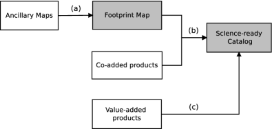
Figure 1: Simplified view of the process of creating a science-ready catalog showing the input data products (open rectangles), and the output data products (filled rectangles). The main steps involved are (a) region selection, (b) object selection and column selection, and (c) the addition of value-added quantities to the final catalog.

Figure 1 illustrates the process of creating a science-ready catalog. In addition to the co-added products released by DESDM (the objects catalog and the mangle mask), other data products like ancillary maps and value-added products are required. The ancillary maps are used in the region selection step and the result of the combination of those maps is the footprint map associated with the final catalog. When combined with the co-added objects table, the footprint map removes objects in regions affected by artifacts (such as bright stars, foreground galaxies, and globular clusters), and set the catalog area based on constraints applied on depth and other survey parameters. Constraints on the object sample like magnitude cuts, signal-to-noise cuts, color cuts, and quality flags are applied in the object selection step. Finally, only the relevant columns for a particular analysis are selected from the objects table. Other properties like photometric redshifts (photo-$z$s), as well as parameters from the ancillary maps, can be added to the final catalog. The result of this approach is an efficient tool that can be used by the scientist to automate the creation of science-ready catalogs, and test the impact of the different inputs and configurations on the science results.

In the catalog infrastructure, a relational database stores an inventory of the input data products, and all steps above are implemented through SQL queries. A large number of tables and configuration parameters often result in complex SQL queries and optimization problems. This issue motivated the development of a module called uery_builder }. The {\verb uery_builder creates the SQL queries for the scientist through a graphical user interface that simplifies the selection of the input data and the catalog configuration. Once a catalog is created, the selected input data, the configuration and the SQL queries executed are registered in the database and associated with the process that created the catalog. The characterization of the final catalog is then performed by another module, atalog_properties }, whih creates plots of the projected distribution, number counts, color-color, color-magnitude, star–galaxy separation and photo-$z$ distributions depending on its application.

There are specific pipelines implemented in the portal to create science-ready catalogs, they share the same infrastructure but the input data and the configuration are different in each case. The science-ready catalogs are divided into three categories: i) lightweight catalogs designed to feed the science analysis pipelines (see Sections  4 and  5) ii) generic catalogs that can be created with the same infrastructure but used for analysis outside the portal (see Section  6), and iii) special samples which are derived from i) with further selection criteria (see Section  7).

The reader should note that the results and statistics presented in this paper are meant to illustrate the portal infrastructure. While the services are provided to all DES collaborators, they are not necessarily the source of the science-ready catalogs used for every DES publication.

3 Data products

Currently, the portal is running at the Laboratório Nacional de Computação Científica (LNCC). As part of the DES public data release (DR1) effort, we plan to migrate some of the portal services to NCSA. In the meantime, the co-added products released by DESDM must be transferred to LNCC and uploaded into the portal. This task is done in an early stage called Data Installation.

For the DES Year 1 Annual Release (hereafter, Y1A1), some data products derived from the single epoch data or the co-added products, such as the ancillary maps and value-added products, were created by the portal during an intermediate stage called Data Preparation, while others were prepared by the DES collaboration and uploaded. Ideally, all data products would be created through the portal for rapid turn around when new data releases are available. Our expectation is to create the data products increasingly through the portal, as the survey science collaboration matures.

In the portal, the co-added products are organized by Data Release (in this case Y1A1) and Data Set. Data Set corresponds to independent fields in this release such as the wide fields overlapping the SDSS Stripe 82 (S82) region, the South Pole Telescope region [SPT, Carlstrom et al., 2011], and the supplemental fields at different depths.

3.1 Co-added products

DESDM provides the co-added objects catalog and the footprint masks in the mangle [Swanson et al., 2012] format. The Y1A1 co-added objects table contains 139,142,161 unique objects spread over 1,800 deg² in two wide regions S82 and SPT. The Y1A1 co-adds are combinations of up to 5 exposures in each of the $grizY$ filters. The typical coverage across the footprint is about $N=3.5$ exposures in each filter.

Y1A1 also contains supplemental fields. Many individual exposures of the DES Supernovae fields (C, S, X, E), the COSMOS [Scoville et al., 2007] fields, and the VVDS14 [Le Fèvre et al., 2005] fields were obtained during year-1 observations and DES Science Verification (SV). These exposures have been co-added into three sets of $90$ tiles in three separate depths: D04 (similar to the depth of the Y1A1 S82 and SPT regions), D10 (equivalent to $N=10$ representing a 5-year completed survey depth) and DFULL (with all exposures available from SV and year-1). In each set, there are 74 SN tiles, 8 COSMOS tiles, and 8 VVDS14 tiles. The supplemental fields are used for the creation of training sets for photo-$z$ algorithms [Gschwend et al., 2017].

The Y1A1 mangle masks have about $10^{8}$ distinct polygons representing the detailed geometry of the observations and the co-addition, keeping information about co-added weight, effective area, magnitude limit and exposure time of the survey as a function of the position on the sky. Another mask, the bit mask, is used to eliminate objects that overlap bright stars and bleed trails, also represented as mangle masks.

3.2 Ancillary maps

In addition to the co-added products, ancillary maps were produced to characterize the coverage, depth and observing conditions of the survey. An important result of the process of creating a science-ready catalog is the footprint map which is created by combining several ancillary maps.

The Y1A1 ancillary maps are Hierarchical Equal Area isoLatitude Pixelation [HEALPix, Górski et al., 2005] representations of the survey characteristics as described by Drlica-Wagner et al. [2018]. By default, we use NSIDE=4096 corresponding to a pixel area of 0.73 arcmin². HEALPix supports two different numbering schemes for the pixels, NESTED and RING; in the current implementation only RING is used. While the HEALPix maps are not exact representations of the survey characteristics they are computationally fast and convenient for creating the footprint map, in particular when several maps with different constraints are used (see Section  4.1).

We can summarize the ancillary maps used during the creation of a science-ready catalog as:

• Coverage fraction map (hereafter, detfrac maps) are used in the region selection step to remove non-observed regions and to compute the catalog area. They are created at the working resolution of NSIDE=4096 by computing the fraction of subpixels at higher resolution (NSIDE=32768, pixel area of 0.01 arcmin²) that are contained within the mangle mask [Drlica-Wagner et al., 2018]. For example, a pixel with DETFRAC_I=0.8 at NSIDE=4096 means that 80% of its area has been observed.

• Bad region mask is designed to remove catalog artifacts like unphysical colors, astrometric discrepancies, bright stars, large foreground galaxies and bright galaxies. See Table 1 for a list and description of the flags used. For the complete description of each flag and the criteria used to define the area removed by the various flags see Drlica-Wagner et al. [2018]. When the bad region mask was first used in association with the Cluster Finder pipeline in the portal, we noticed a significant number of spurious galaxy cluster detections due to globular clusters. Thus we added a flag based on the globular cluster catalog of Harris [1996, 2010 edition] to remove those regions. In the future, we propose to separate the current bad region mask in two, one to flag artifacts associated with the release and another one to flag regions affected by Foreground Objects, so that these products can be created independently and the Foreground Objects mask reused in subsequent data releases.

• Survey depth maps give the magnitude limit at 5-$\sigma$ and 10-$\sigma$ as a function of position on the sky for the AUTO and APER4 magnitudes [Rykoff et al., 2015].

• Systematics (or survey conditions) maps contain the total exposure time, mean seeing, mean air mass and sky background in each of the $grizY$ filters. Their creation is implemented in the portal following the prescription of Leistedt et al. [2016].

Table 1: Bad region mask flags.

Flag #	Description
1	High density of astrometric discrepancies
2	2MASS moderate star regions ($8<J<12$)
4	RC3 large galaxy region ($10<B<16$)
8	2MASS bright star region ($5<J<8$)
16	Region near the LMC
32	Yale bright star region ($-2<V<5.6$)
64	High density of unphysical colors
128	Globular cluster regions from Harris [1996, 2010 edition] catalog

3.3 Value-added products

The value-added products used as input to create catalogs are the zeropoint correction, photo-$z$s, star-galaxy separation and galaxy evolution properties computed in the Data Preparation stage for each object in the co-added objects table. Table 2 summarizes the data products and the properties stored in the database for each value-added product.

3.3.1 Zeropoint correction

The Y1A1 data is calibrated using a Global Calibration Module (GCM) developed by DES, which follows the procedure of [Glazebrook et al., 1994] adapted to DES by Tucker et al. [2007]. However, internal studies have shown that Y1A1 residual calibrations uncertainties at the level of 2% persist. A stellar locus regression (SLR) solution has been applied to the data for zeropoint calibration, following the prescription detailed in Ivezić et al. [2004] and MacDonald et al. [2004].

In the portal, the zeropoint correction includes the correction of the magnitudes by extinction [SFD98 Schlegel et al., 1998], and finding an SLR solution at the scale of a DES tile ($0.5$ deg²) using a modified version of the BigMACS SLR code [Kelly et al., 2014].

Differences in calibration might affect color cuts, photo-$z$ estimations, and the star-galaxy separation. Therefore, the same calibration must be applied consistently to the different data products that are used as input to create a science-ready catalog. Photometric consistency is ensured by the provenance scheme built into the portal. For future DESDM data releases, different calibration techniques might be applied reinforcing the importance of keeping track of this information.

3.3.2 Photo-zs

The pipelines implemented in the portal to compute the photo-$z$s are fully described by Gschwend et al. [2017]. The steps involved are summarized below:

• creation of a spectroscopic database, currently with redshift measurements for a total of 31 galaxy spectroscopic surveys available in the literature, and 759,890 unique, high-quality spectroscopic redshifts;

• creation of a spectroscopic sample by combining the surveys, homogenizing the data and resolving multiple redshift measurements of the same source;

• matching of the spectroscopic sample with the co-added objects table used as input to create training and validation sets;

• training of the photo-$z$ algorithms;

• calculation of the photo$z$s with the three algorithms used in this paper: DNF [De Vicente et al., 2016], LePhare [Arnouts et al., 2002] and MLZ/TPZ [Carrasco Kind and Brunner, 2013, 2014].

For interoperability among the different algorithms, the original property name in the output of each algorithm is translated to the portal’s internal format when the database table is created. The name of the algorithm used is registered along with other metadata associated with the process.

Even though some photo-$z$ algorithms compute Probability Density Functions (PDFs) it can be computationally very expensive to store them for all the objects in the co-added objects table [e.g., Carrasco Kind and Brunner, 2014]. Within the portal, one way to alleviate this is to compute and store photo-$z$ PDFs for the science-ready catalogs or Special Samples (see Section 7) which are reduced in size compared to the whole sample.

Table 2: Description of the value-added products and their properties stored in the database in the Data Preparation stage.

Zeropoint correction
COADD_OBJECTS_ID	Unique object identifier
SLR_SHIFT	SLR magnitude shifts for each of the $grizY$ filters
EXTINCTION	Extinction for each of the $grizY$ filters
Photo-$z$s
COADD_OBJECTS_ID	Unique object identifier
Z_BEST	Best estimate of the photo-$z$
ERR_Z	Photo-$z$ error
Star-galaxy separation
COADD_OBJECTS_ID	Unique object identifier
CLASS_STAR	Star-galaxy classification$\dagger$ ($0=$ galaxy and $1=$ star) for each of the $grizY$ filters
SPREAD_MODEL	Star-galaxy classification$\ddagger$
MODEST	Star-galaxy classification$\diamondsuit$, v1 and v2 which are based on the SPREAD_MODEL
Galaxy evolution properties
COADD_OBJECTS_ID	Unique object identifier
Z_BEST	Best estimate of the photo-$z$
MAG_ABS	Absolute magnitude
K_COR	k-correction
DIST_MOD_BEST	Distance modulus
MASS_BEST	Stellar mass for the best galaxy model
SFR_BEST	Star-formation rate for the best galaxy model
AGE_BEST	Age of stellar population for the best galaxy model
EBV_BEST	Internal extinction for each of the $grizY$ filters
$\dagger$ Bertin and Arnouts [1996]
$\ddagger$ Desai et al. [2012]
$\diamondsuit$ Chang et al. [2015]

3.3.3 Star-galaxy separation

The star-galaxy separation algorithms developed by the collaboration are described by Sevilla-Noarbe et al. [2018]. Five algorithms are currently implemented in the portal: CLASS_STAR [Bertin and Arnouts, 1996], SPREAD_MODEL [Desai et al., 2012] and Y1A1 MODEST v1 and v2 [e.g., Chang et al., 2015] which are also based on the SPREAD_MODEL parameter. So far, those star-galaxy separation algorithms use only morphological information. Thus the classification is indeed between extended and point sources, referred here as galaxies and stars respectively. However, the infrastructure can be extended to include other classes of objects, e.g., QSO, as other classification algorithms are implemented. As in the case of other value-added products, the output of each algorithm must be translated to a common format within the portal to ensure interoperability.

3.3.4 Galaxy evolution properties

For galaxy evolution studies, galaxy properties are computed by the LePhare [Arnouts et al., 2002] algorithm at the redshift Z_BEST computed either by LePhare itself or by another photo-$z$ algorithm implemented in the portal. The galaxy evolution properties for the best magnitude model solution based on the Spectral Energy Distribution (SED) used as template are listed in Table 2 as well.

4 Use case example: lightweight catalog for Large Scale Structure

To illustrate the creation of a science-ready catalog in the portal, we use as an example a lightweight magnitude-limited catalog adequate for computing the angular correlation function. The portal graphical user interface helps the user select the input data and configuration (see  B). For the Large Scale Structure (LSS) pipeline, the data products presented as input to the user are the co-added objects table, the star-galaxy separation and the photo-$z$ tables for the different algorithms implemented in the portal. By selecting those products, the methods for star-galaxy separation and photo-$z$ are immediately set. Once the input data are selected, the user has the chance to change the default configuration parameters for the LSS catalog before submitting a process in the portal. At this point, the input data and the configuration used are saved and associated with the new process.

Next, we describe in detail how the uery_builder } performs the \textit{region selection}, \textit{object selection} and \textit{column selection} steps to create the LSS catalog (see Figure ~\ref{fig:uery_builder). In the  A we present the SQL queries created for this particular example.

4.1 Region selection

We start by creating a footprint map as the result of the constraints applied to the detfrac maps, bad region mask, systematics maps and depth maps.

For the LSS default configuration (see Table 4), only pixels with DETFRAC_I $>0.8$ are selected. The bad region mask with FLAG=2,4,8,32,128 ensure that regions affected by bright stars, large foreground galaxies, and globular clusters are removed from the catalog. From the systematics maps, we use the exposure time map to select pixels with EXPTIME $>=90$s in each of the $griz$ filters . In this example, we keep only pixels in the depth map with magnitude limit $i>22$, so that our final catalog can include galaxies with signal-to-noise of 10 $\sigma$ or higher at magnitudes brighter than $i=22$ . The appropriate depth map is chosen from the selected resolution (NSIDE=4096), magnitude-type (MAG_AUTO) and signal-to-noise of the limiting magnitude (10$\sigma$). The current infrastructure relies on the depth maps created by the collaboration that includes SLR adjustments and extinction correction (see details in Drlica-Wagner et al. [2018]). Therefore, in order to be consistent, the magnitudes used in the preparation of training sets, in computing photo-$z$s and listed in the final catalog must be corrected accordingly. This need shows the importance of having the depth maps also created through the portal for self-consistency.

4.2 Object selection

The resulting footprint map is then combined with the co-added objects table, which removes about $16\%$ of the objects in this operation. For the LSS default configuration (see Table 5), the selected sample includes objects with magnitudes $17.5<i<22$; colors $-1<g$-$r<3$, $-1<r$-$i<2.5$, $-1<i$-$z<2$, $-5<z$-$Y<5$; and SExtractor quality FLAG $=0$, $1$, and $2$ in the $i$-filter. As discussed in the region selection step, in this example only pixels with DETFRAC_I $>0.8$ are kept. Then the mangle mask in the $i$-filter must be applied to make sure that the objects in the selected pixels that overlap the mangle mask are properly removed.

Still in the object selection step, there are additional cuts that are applied by default to remove artifacts associated with stars close to the saturation threshold, objects with bad astrometric colors and objects with unphysical colors (see details in Drlica-Wagner et al. [2018]).

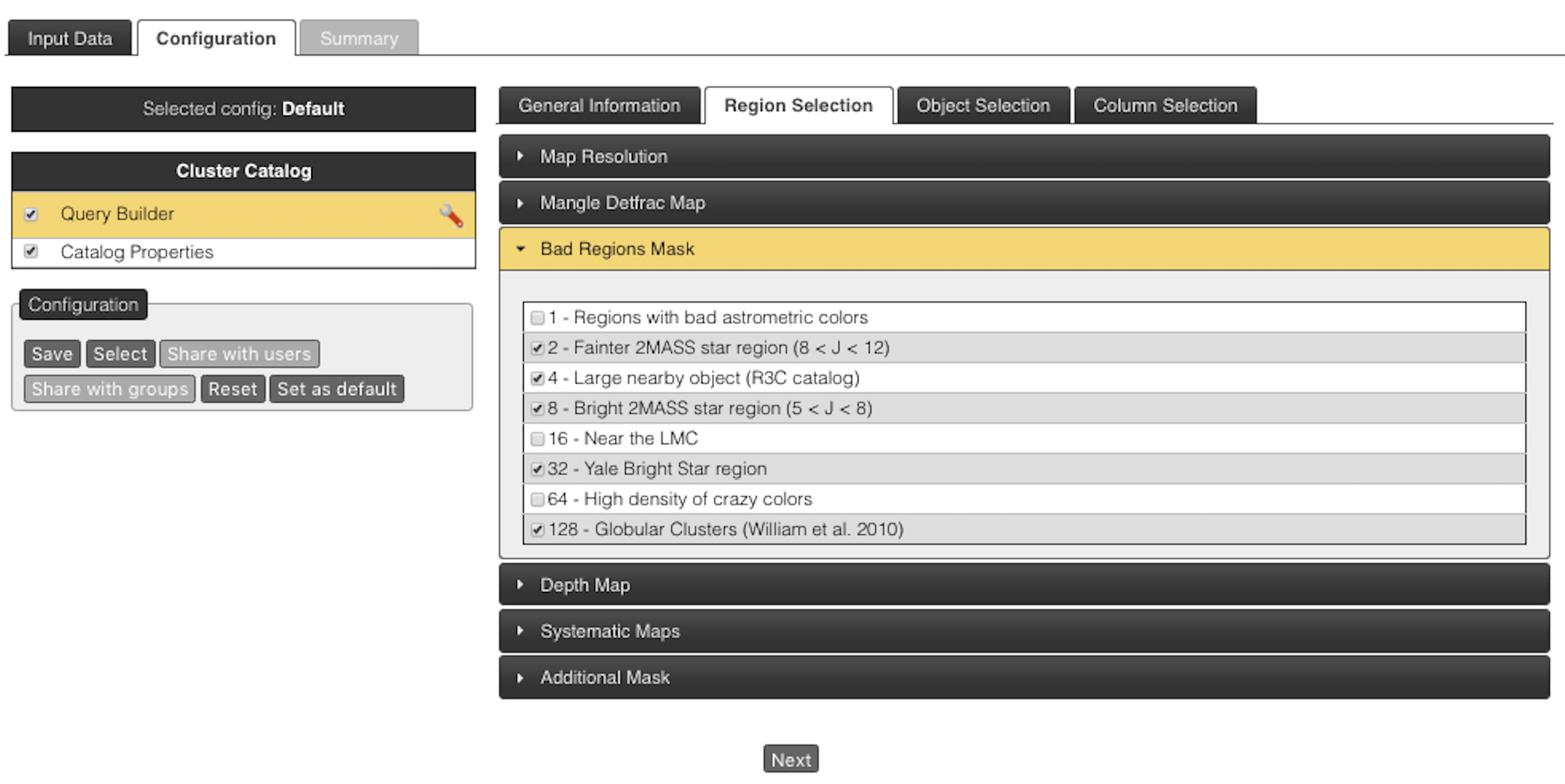
Figure 12: Configuration manager interface showing the configuration of the region selection, one of the steps executed during the creation of a science-ready catalog.

The resulting object sample is then combined with the Y1 MODEST v2 star-galaxy separation table to select objects classified as galaxies using the value of the classifier in the $i$-filter as a reference. As in the region selection step, all these parameters are presented in the configuration interface and can be changed by the user (see Figure 12).

4.3 Column selection

For the LSS lightweight catalog, a few columns are selected by default. These are called system default since they are required to feed the science analysis pipelines that use this catalog. The columns are: COADD_OBJECTS_ID, RA, DEC, MAG_[GRIZY], MAGERR_[GRIZY], Z_BEST and ERR_Z with magnitudes and errors consistent with the magnitude type selected in the object selection configuration. Still in the column selection step, additional columns from the co-added objects table, value-added products or ancillary maps can be selected in the configuration interface and added to the final catalog.

The execution time for the region selection, object selection and column selection steps is roughly proportional to the number of objects in the co-added objects table. In this example, the execution time for the S82 region (334 tiles) was 00h22m while for SPT (3,373 tiles) it was 02h45m. It is important to note that the overall execution time to create a science-ready catalog was significantly reduced also because the value-added products were previously computed for all the objects in the co-added objects table. In that process, the photo-z estimation is the most time consuming step [see Gschwend et al., 2017].

Table 3: Properties of the S82 and SPT magnitude-limited catalogs.

Catalog	Footprint Area	Ngals	Mean Density
	(deg2)		(gal arcmin-2)
S82	140.65	1,806,274	3.57
SPT	1,375.48	17,915,328	3.63

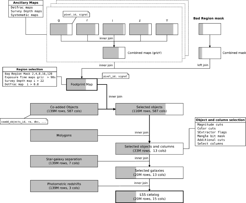
Figure 2: Representation of the SQL operations executed during the creation of the LSS lightweight catalog described in Section 4. Rectangles are input data or temporary tables created along the process. The ancillary maps on the top are combined to create maps with constraints on the detfrac, survey depth and systematics maps parameters. The combined maps are then joined with the bad region mask to create the footprint map. The shaded area represents qualitatively how the size of the catalog is shrinking (number of rows and columns) in each step. The join of the footprint map with the co-added objects table removes a large number of objects, speeding up the subsequent object selection step. Joins with the value-added products and the co-added objects sample are done only at the end, operating on a reduced object sample for efficiency. The resulting catalog is optimized for its science application.

4.4 Characterization of the catalog properties

After creating a catalog, the portal performs an automatic characterization of its properties. In this section, we illustrate some of the results of this characterization applied to our LSS lightweight catalog.

The basic properties of our LSS lightweight catalog are listed in Table 3 which gives the area of the final footprint, the number of galaxies and the mean density of galaxies per arcmin² in the final catalog. The projected density distribution is shown in Figure 3. Close inspection of the table and figure indicates that the catalogs are pretty uniform across the sky, and have similar mean number densities, differing by less than 1%.

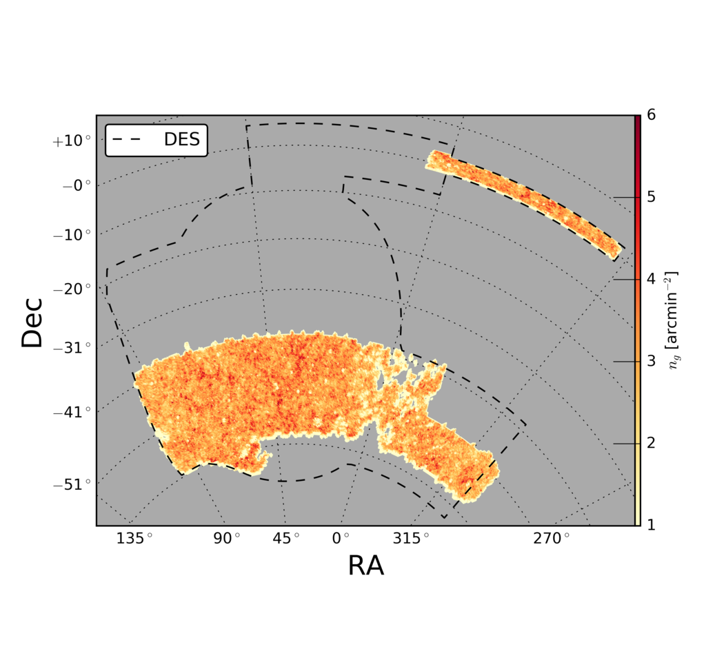
Figure 3: Projected density distribution for the S82 (around Dec$=0^{\circ}$) and SPT (-60${}^{\circ}<$ Dec $<-40^{\circ}$) regions of the lightweight LSS catalog.

In Figure 4 we compare the $i$-band magnitude distributions for both S82 and SPT regions with those obtained by other authors, normalized to the same area. We find excellent overall agreement between the counts of the two independent regions and consistency with the counts of the other authors despite possible differences in the $i$-filter used.

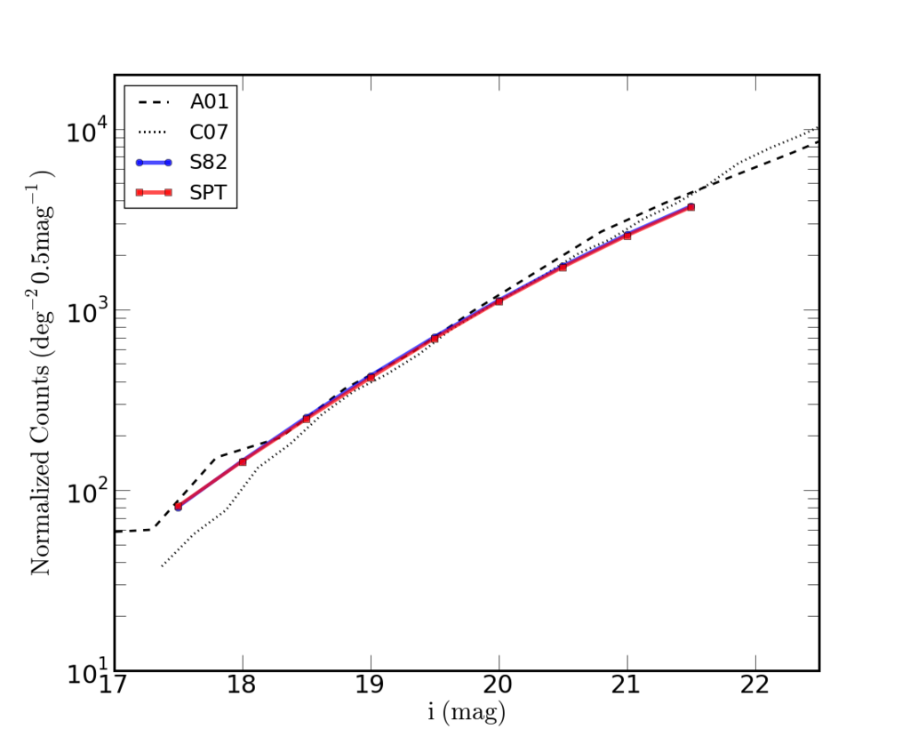
Figure 4: Normalized counts of galaxies in the $i$-band for the S82 and SPT magnitude-limited catalogs. We also show results obtained by other authors: A01- Arnouts et al. [2001], and C07- Capak et al. [2007].

Figure 5: Distribution of photo-$z$s computed by the MLZ/TPZ algorithm for the S82 (blue line) and SPT (red line) magnitude-limited catalogs. The gray histogram represents the distribution of VVDS spectroscopic survey for the same magnitude limit ($i=22.0$).

The photo-$z$ distribution computed by the MLZ/TPZ algorithm for the S82 and SPT regions is shown in Figure 5. From the figure we see that the photometric distributions of the two regions are similar and in reasonable agreement with that of VVDS spectroscopic survey limited to the same magnitude, except by the excess in the 0.3-0.5 interval.

We conclude that the automatic characterization built on the portal is useful to quickly assess the self-consistency of catalogs created with the same configuration but using different input data. In this case, the disjoint S82 and SPT regions in Y1A1 demonstrates the overall uniformity of the survey, and the good agreement with the results of other surveys.

The automatic characterization, as well as the record of the input data and configurations, are especially important when multiple catalogs are created, as discussed in Section 4.5.

4.5 Creating multiple catalogs

Our LSS lightweight catalog was created using specific star-galaxy separation and photo-$z$ algorithms. In order to explore the possible impact of these choices on the science results, we demonstrate the value of the portal in creating multiple catalogs for the S82 region by changing the methods used for separating stars and galaxies and for computing photo$z$s.

The effects of using different methods for separating stars and galaxies can be examined in Figure 6, which shows the variation of the projected density of galaxies as a function of the galactic latitude, $b^{\textsc{ii}}$. The methods used were CLASS_STAR, SPREAD_MODEL and Y1 MODEST v2. They show a rapid rise in the density for galactic latitudes below $b^{\textsc{ii}}\sim-35^{\circ}$, suggesting some degree of contamination by stars wrongly classified as galaxies. Although it is not a quantitative way to establish the best star-galaxy separation algorithm, it at least shows that our choice was reasonable given the alternatives.

Similarly, to assess the impact of using different photo-$z$ algorithms we show in Figure 7 the redshift distribution for three catalogs created using MLZ/TPZ, DNF and LePhare for the SPT region. From the figure, we find that the empirical methods yield similar results over the entire range. They contrast with the SED fitting method which deviates considerably from the empirical methods for $z<0.5$. Interestingly, all methods yield very similar distributions for $z>0.7$.

The important point is that the present infrastructure allows the user to generate different catalogs quickly, feed the science analysis pipelines implemented in the portal with those catalogs and evaluate the impact that different inputs and configurations have on the scientific results. Something like that would be costly to do by hand especially with the increasing volume of data. In addition, the same infrastructure could be easily adapted to create catalogs from simulated data in order to assess the performance of the star galaxy-separation and photo-z algorithms against a truth table.

Figure 6: Impact of different star-galaxy separation algorithms in the density of galaxies as a function of the galactic latitude, $b^{\textsc{ii}}$.

Figure 7: Distribution of the photo-$z$s computed by the MLZ/TPZ (red), DNF (blue) and LePhare (green) algorithms for the catalog described in Section 4 for the SPT region.

5 Other lightweight catalogs

In section 4 we described how we use the portal to create a lightweight catalog adequate for LSS studies with just the columns required to compute the angular correlation function in the portal. The uery_builder } is flexible enough to create catalogs for different applications, changing only the input data products and the configuration used. As in the case of LSS, catalogs for \textit{Galaxy Clusters} (Cluster), \textit{Galaxy Evolution} (GE) and \textit{Galaxy Archaeology} (GA) are also lightweight and designed to feed the corresponding analysis pipelines in the portal ready to be used and with only the reuired columns. The default configuration for the lightweight catalogs is summarized in  A. As explained in Section 8, the user can change and save specific configurations for each pipeline using the Configuration Manager user interface.

For cluster studies, we created catalogs (similar to the LSS ones) to feed the Cluster Finder pipeline implemented in the portal. This pipeline uses the Wavelet Z Photometric [WAZP Benoist, 2018] cluster-finding algorithm, which is based on the 3D spatial clustering considering both the projected distribution of galaxies and their photo-$z$ distribution. The default Cluster catalog has the same columns as the LSS one, and the only differences in the configuration are in the bright magnitude and color cuts, as shown in  A.

For galaxy evolution studies, we have created magnitude-limited catalogs adding columns from the galaxy properties table (see Section 3.3) containing estimates for the stellar mass, absolute magnitude, star-formation rate, spectral type, age of stellar population, internal extinction and k-correction. The GE lightweight catalog presented here was created for the S82 dataset using the PEGASE2 set of spectral energy distribution (SED) to estimate galaxy stellar masses.

In this example, the photo-$z$s are from the MLZ/TPZ algorithm, which were used by LePhare to compute the galaxy properties. The star-galaxy separation method used was Y1 MODEST v2. The apparent magnitude limits were $17.5<i<22.0$, resulting in a sample with 1,357,319 galaxies with absolute magnitudes in the range $-25<M_{i}<-14$ covering 143.76 square degrees.

Figure 8 illustrates some of the properties of our default GE catalog, showing distributions of absolute magnitudes and stellar masses and their dependence with the photo-$z$s. The catalog contains objects from $10^{7}$ to $10^{12}$ M_⊙, with the mass distribution peaking at $10^{10.5}$ M_⊙. The ages cover the range of $\sim$100 Myr to 13 Gyr.

In the future, we plan to include other SED libraries (e.g. [Bruzual and Charlot, 2003] in the portal and Maraston [2005]), in addition to PDFs associated with the photo-$z$s to better estimate their uncertainties and the impact on the luminosity and mass functions.

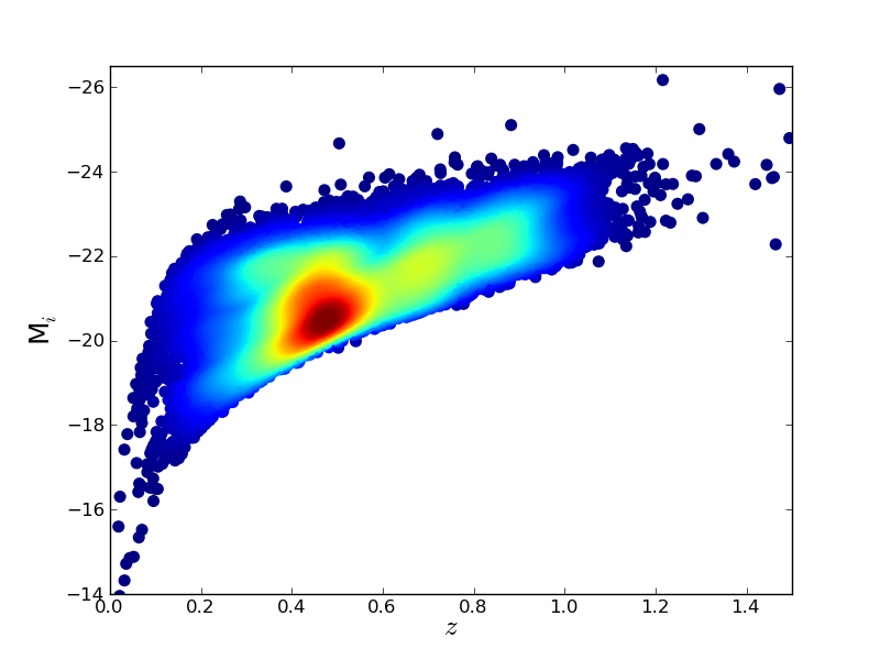
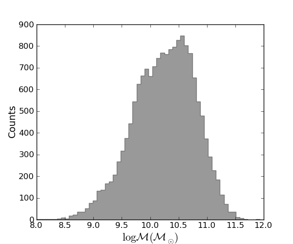
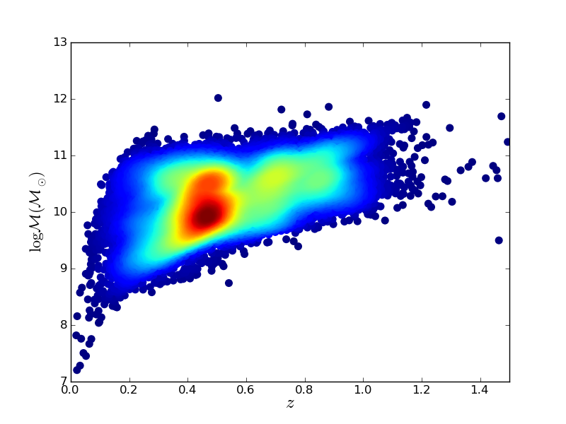
Figure 8: Properties of the lightweight GE catalog using default configuration as described in Section 5. Upper panels: distribution of absolute magnitudes and its dependence with the photo-$z$s; Lower panels: stellar mass distribution and its dependence with the photo-$z$s.

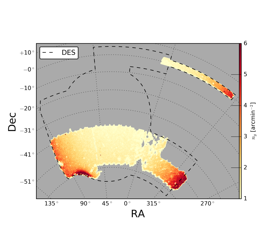
Figure 9: Density map of the lightweight GA catalog created to feed the SPARSEx pipeline as described in Section 5

For GA studies, we created catalogs using two different configurations to feed the SPARSEx and MWfitting pipelines. These pipelines are also being integrated into the portal and are briefly described in the following.

The SPARSEx pipeline is used to detect stellar systems such as globular clusters and nearby dwarf galaxies and has been successfully used with both single-epoch and co-added data [Luque et al., 2016, 2017]. It applies a matched filter technique using data from the color-magnitude diagram (CMD) to build maps of stellar overdensities associated with different simple stellar population models. These overdensities are then detected in the maps and ranked according to their amplitude. Those overdensities most conspicuous and robust to variations in the model parameters are then inspected by eye and have their density profiles, and CMDs analyzed. By default the pipeline uses WAVG_MAG_PSF magnitudes for the object selection step and the Y1 MODEST v2 for star-galaxy separation. The catalog to feed SPARSEx is limited at $r=23$ at $10\sigma$. In this case, the depth map used was based on an aperture magnitude, without extinction correction. In Figure 9 we show the footprint and the projected density distribution of this catalog.

The MWfitting pipeline was developed to study the structure of the Galaxy. It uses models from TRIdimensional modeL of thE GALaxy [TRILEGAL, Girardi et al., 2005, 2012], whose color-magnitude diagrams are computed for different structural models of the Galaxy and a best-fit solution to the observed CMDs is found based on automatic optimization algorithms. The catalog to feed this pipeline requires the selection of regions brighter than a user-specified magnitude in $r$ and $g$ filters to ensure completeness in the $g$-$r$ color. In this case, we used the depth maps in $r$ and $g$ filters, again without extinction correction. We note that like in the previous lightweight catalogs described in this section, the selected columns are just the ones required for the analysis and are listed in A.

6 Generic catalog

The available infrastructure also allows for the creation of generic catalogs suitable to be used outside the portal. For instance, these catalogs may have multiple photo-$z$s, star-galaxy classifications, and galaxy properties, leaving the decision about which method to use to the user. The region selection and object selection steps are still performed but neither star-galaxy classification nor photo-$z$s limits are applied. Additional columns chosen from the co-added objects table and properties associated with the various ancillary maps can be added to the catalog in this column selection step.

The default configuration for a generic catalog proposed in A is the one that creates a magnitude-limited galaxy catalog. Note that because a generic catalog might have more columns by construction and because star-galaxy separation is not applied, they are, generally, larger in size than the lightweight catalogs by a factor of two or more. However, they can still be an interesting option to enable users to carry out their science analysis outside the portal.

7 Special samples

In addition to the lightweight and generic catalogs described above, the portal also supports the creation of specialized samples, starting with LSS, Cluster, GE or GA catalogs as input, and applying further selections. For instance, a volume-limited catalog with information about absolute magnitude can easily be created from the GE catalog. Other use cases are the creation of Emission Line Galaxies or Luminous Red Galaxies samples using selection criteria proposed by Comparat et al. [2016] and Prakash et al. [2016], respectively.

As mentioned earlier, at this point one may also re-run photo-$z$ algorithms to store the PDF which is considerably more efficient given the reduced object sample. For instance, the lightweight GE catalog presented in Section 5 has about $37\%$ of the original co-added objects used to compute point-value photo-$z$s. With this pipeline, it is also possible to combine those samples with other surveys available in the portal (such as WISE and VHS) and complement the DES data with near-infrared photometry. Again, the join operations in the database and positional matching work faster on reduced object samples.

8 Operational benefits of the infrastructure

The infrastructure presented here was designed primarily to prepare catalogs to feed the science analysis pipelines hosted by the portal. The underlying idea is to make sure that i) all steps that create the input catalog are done before executing the pipelines; ii) we can control the impact of different inputs and configurations on the science results; and iii) the science analysis pipelines run on lightweight catalogs. This feature is important to reduce the data sizes and maximize performance.

As shown in Sections 4 and 5 there are about fifty parameters defining a particular catalog and several configurations are allowed for each of the LSS, Cluster, GE, and GA pipelines. The portal has a configuration manager used to save, load and share all these different configurations. These configurations are also part of the provenance of a given portal product.

Since the execution time of some processes may be very large, upon submission of a process the user is notified by e-mail, which contains information about the process. The same happens at the completion of the process when the user receives another notification with concise information about the configuration used, input and output data and links to pages displaying the configuration and the product log. The product log is a compilation of information about the current process and links to the previous ones that generated the input data. These links allow the user to access the whole chain of preceding processes, again including information about the inputs, configurations, version of the codes used, as well as plots and tables describing the results of the process in the chain.

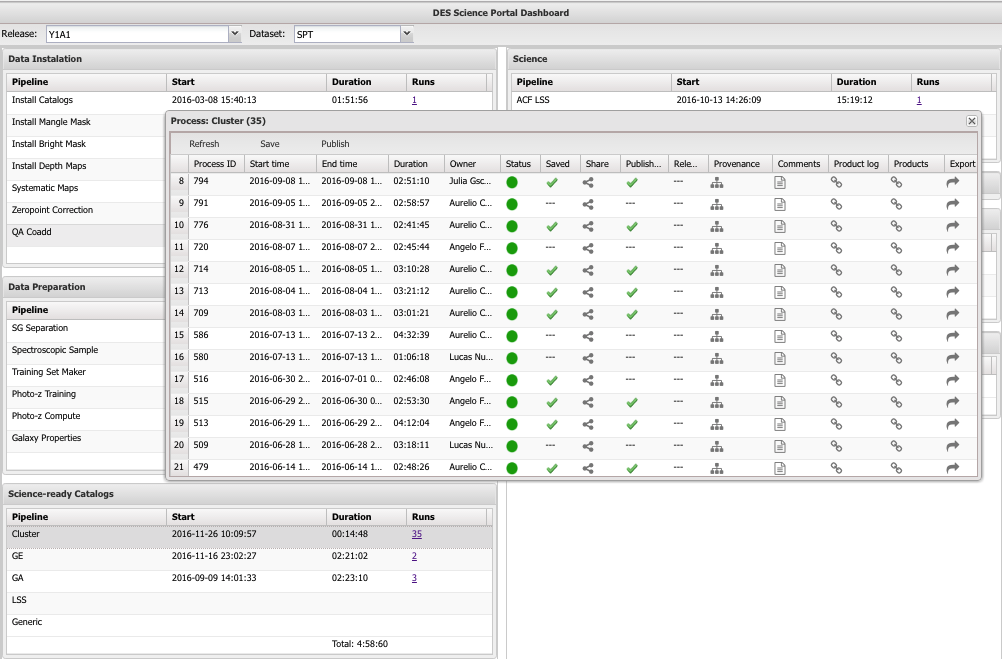
Figure 13: Dashboard interface showing the pipelines implemented in the portal and their stages. The pop-up lists all the processes that created Cluster catalogs for the Y1A1 Data Release and SPT Dataset and the associated information available for each process.

Products from a given pipeline are assigned a running number which provides a unique identification for the Data Release and Data Set in addition to the name chosen by the user. Products can be published, and in this case, they automatically appear in an interface called Science Products, which users can download them (see  B). Similarly, processes and products can be accessed from a dashboard available to the operator and system administrators but in contrast to the Science Products interface all processes are registered, even the ones that failed, thus providing a complete history of the pipeline executions. The dashboard used to monitor the execution of each pipeline in the portal is shown in Figure 13. In the first tier, it shows the start time, duration and status of the latest run. In the second tier, it provides access to all previous runs with links to the product log and the data products created by each process in a third tier.

Currently, the catalog production described in this paper is only available at LNCC instance of the portal. Nevertheless, all products can be made available via a Science Products interface being developed at NCSA. This procedure is done by using the export tool that transfers any data product created by the portal to NCSA creating the corresponding table in the DES Science database.

9 Future developments

While the current infrastructure has been extensively tested and is already in operation, a number of improvements are necessary to keep the portal current with the algorithms and procedures defined by the DES collaboration. Some of them are:

• Improve the Install Catalogs pipeline not only to transfer and ingest the co-added products released by DESDM but also distribute the data among the cluster nodes partitioning the data using HEALPix.

• Implement the local creation of depth maps. These are currently being created by the DES collaboration and uploaded to the portal. Local implementation would also allow the portal to be more flexible, enabling the creation of depth maps at different signal-to-noise ratios, with or without extinction correction and for different magnitude types.

• Separate the current bad region mask into two, one to flag artifacts associated with the release and the other to flag regions affected by foreground objects, so that these products can be created independently and the foreground objects mask reused in subsequent releases.

• Include other methods for computing photo-$z$ and star-galaxy separation as suggested by the DES collaboration.

• Extend the training of photo-$z$ samples based on multi-band photometric data to complement the infrastructure based on spectroscopic samples.

• Introduce additional SEDs to calculate galaxy properties.

• Store $z_{MC}$, a Monte Carlo value sampled from the photo-$z$ PDF, and store a compressed representation of the PDF for each object as well.

• Expand the number of queries available in special samples.

• Use of ancillary maps to create more realistic catalogs based on simulations.

• Enable the download of data products through the Science products interface, in collaboration with the DESDM group at NCSA.

• Ability to run the query_builder in the Jupyter environment. We plan to implement the configuration interface, as well as the plots and tables for the catalog characterization in a Jupyter notebook.

In addition to these specific short-term goals, we are currently adapting the uery_builder } to work with other database engines using \texttt{SQLAlchemy}\footnote{\url{http://www.slalchemy.org/. This action is an important step to migrate the catalog infrastructure to NCSA and integrate it with the DES Science database. We are also constantly reviewing the portal code base and evaluating how to operate the portal in environments other than a dedicated cluster to avoid scalability problems in the future.

10 Summary

In this paper, we describe an infrastructure to create science-ready catalogs implemented in the DES Science portal. The portal creates science-ready catalogs starting from the co-added products released by DESDM, integrating algorithms and procedures developed by the DES collaboration for the Y1A1 data release. The infrastructure uses ancillary maps that describe the survey characteristics, different methods for computing star-galaxy separation, photo-$z$s and galaxy properties.

The input data products and the configurations used are registered in a relational database. The science-ready catalogs are fully created in the database by a set of SQL queries. A module called uery_builder } automatically creates the ueries based on the input data products and configuration selected through the portal user interface. Provenance information is registered for each pipeline of the catalog infrastructure and is accessible through a dashboard interface making the entire process reproducible. We demonstrated the flexibility of the infrastructure by creating lightweight catalogs for LSS, Cluster, GE, and GA to feed science analysis pipelines in the portal, generic catalogs, and special samples.

The portal makes the complex process of creating science-ready catalogs manageable, well-documented and sustainable. While this approach has been primarily motivated to feed the science analysis pipelines being implemented in the portal, the catalogs created can also be distributed for the DES collaboration. Our goal is to migrate this infrastructure to NCSA where the DES data releases are produced, turn it into an operational science environment for the DES collaboration and continue integrating new algorithms and methodologies developed or suggested by the collaboration as the survey progresses.

Appendix A Query builder

The uery_builder } was developed to automatically create the SQL ueries from selected input data and configuration. The concept behind the uery_builder } is that a complex uery can be solved by breaking it down into simpler sub-queries creating temporary tables in the database. This procedure reduces the overall execution time ensuring that the sub-queries are written efficiently forcing the execution of the sub-queries in the right order and not depending exclusively on the database query optimizer.

Figure 2 illustrates how the queries to create the LSS catalog described in Section 4 are built. Because join operations on map tables are much faster than the equivalent operation on object tables, we start by operating on the ancillary maps. As described in Section 4.1, the footprint map is what is left after the removal of pixels that satisfy the constraints imposed by the ancillary maps. The join with the footprint map removes a significant number of objects from the co-added objects table, speeding up the object selection queries that follow. The association between PIXEL_ID and COADD_OBJECTS_ID is done through an auxiliary table created using the PG_HEALPIX Postgresql plugin for the appropriate resolution and ordering schema. In addition, the object selection step is optimized by creating temporary tables with only the subset of columns required to apply the cuts described in Section 4.2. Finally, joins involving large tables (like the co-added objects, the star-galaxy separation, and photo-$z$ tables) are expensive operations. However, performing them in individual subqueries by first removing objects through the object selection cuts, then selecting galaxies and only then joining with the the photo-$z$ table, reduces the execution time significantly. This recipe (including the tables and parameters from the configuration, the operations and the order in which the operations are performed) is encoded in the query_builder. Improvements in the query_builder include expression of the operations in a configuration file to avoid changes in the code to add new operations, and rewrite the code using SQLAlchemy to build the SQL clauses in Python and support different SQL dialects like Postgresql, MySQL, and Oracle.

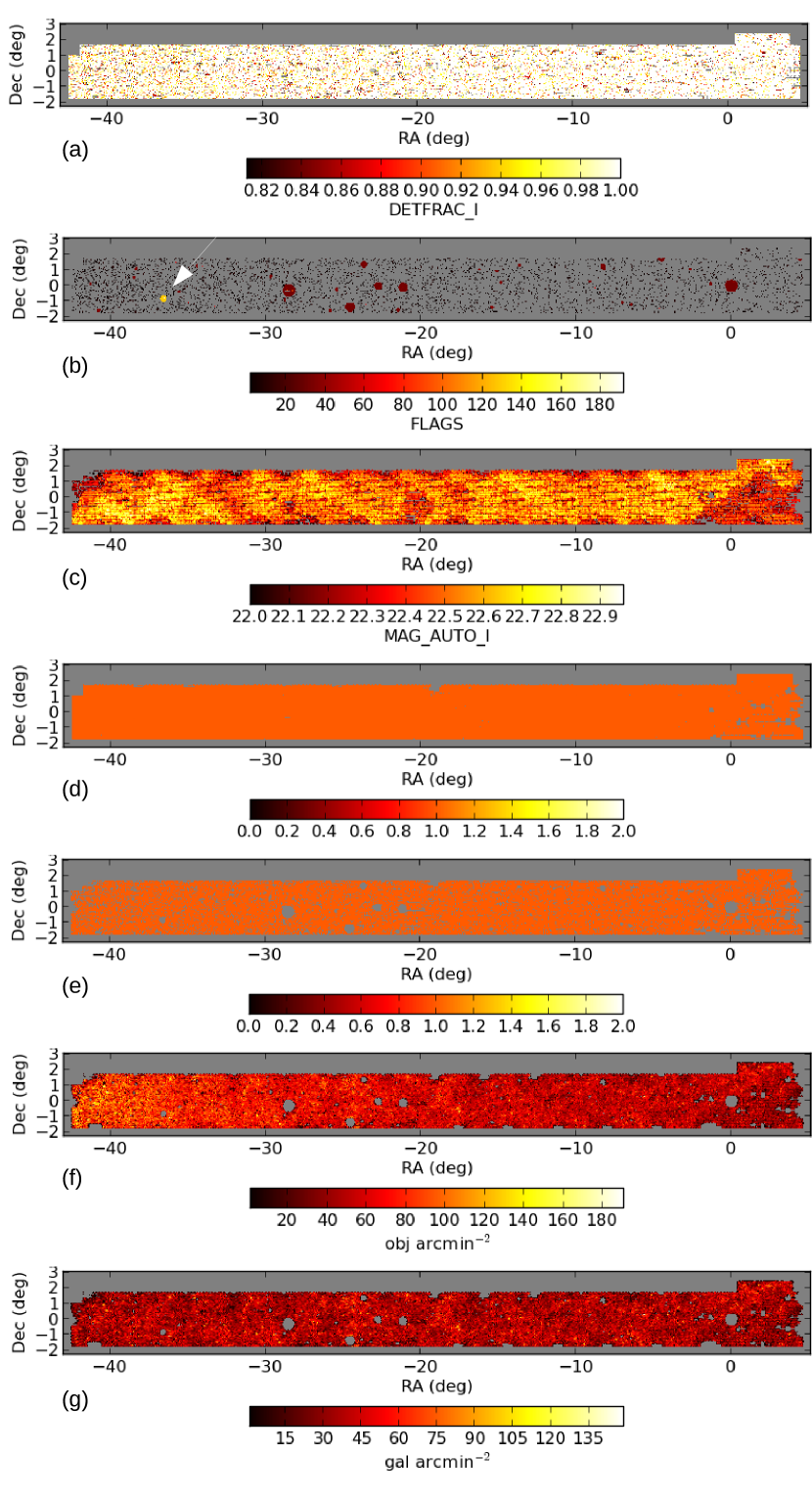
Figure 10: Steps to create the LSS catalog as described in Section 4 for the S82 dataset. Panel (a): regions with DETFRAC_I > 0.8. Panel (b): bad region mask with FLAG=2,4,8,32, and 128. The white arrow indicates the position of the globular cluster M2 removed by the FLAG=128. Panel (c): regions with depth with $i>22$ at 10-$\sigma$. Panel (d): binary map showing regions with EXPTIME $>90$s in the $griz$ filters. Panel (e): footprint map after combining the previous conditions, with a total area of 140.65 deg². Panel (f) map showing the density of objects after the object selection step with 5.89 obj/arcmin². Panel (g): map showing the density of galaxies after the star-galaxy separation step with 3.57 gal/arcmin².

The queries used to create the LSS catalog are presented below and can be inspected together with Figure 10. This figure shows the ancillary maps, the resulting footprint map after the region selection step and the density map of the selected galaxies after the object selection step for the S82 dataset.

1. detfrac map queries:

⬇

CREATE TEMP TABLE <tmp_deftrac_i> AS (

SELECT a.pixel, a.signal, a.ra, a.’dec’

FROM <detfrac_i> a

WHERE signal >= 0.8);

2. Bad region mask queries:

⬇

CREATE TEMP TABLE <tmp_badregion> AS (

SELECT a.pixel, a.signal, a.ra, a.’dec’

FROM <badregion_mfask> a

WHERE (CAST(signal AS INTEGER) & 174) > 0);

3. Depth map queries:

⬇

CREATE TEMP TABLE <tmp_depth> AS (

SELECT a.pixel, a.signal, a.ra, a.’dec’

FROM <depth_i> a

WHERE signal >= 22);

4. Systematic map queries:

⬇

CREATE TEMP TABLE <tmp_exptime_g> AS (

SELECT a.pixel, a.signal, a.ra, a.’dec’

FROM <exptime_g> a

WHERE signal >= 90);

CREATE TEMP TABLE <tmp_exptime_r> AS (

SELECT a.pixel, a.signal, a.ra, a.’dec’

FROM <exptime_r> a

WHERE signal >= 90);

CREATE TEMP TABLE <tmp_exptime_i> AS (

SELECT a.pixel, a.signal, a.ra, a.’dec’

FROM <exptime_i> a

WHERE signal >= 90);

CREATE TEMP TABLE <tmp_exptime_z> AS (

SELECT a.pixel, a.signal, a.ra, a.’dec’

FROM <exptime_z> a

WHERE signal >= 90);

CREATE TEMP TABLE <combined_exptime> AS (

SELECT a.pixel, 1 as signal, a.ra, a.’dec’

FROM <tmp_exptime_g> a

INNER JOIN <tmp_exptime_r> b ON a.pixel = b.pixel

INNER JOIN <tmp_exptime_i> c ON b.pixel = c.pixel

INNER JOIN <tmp_exptime_z> d ON c.pixel = d.pixel);

5. Footprint map queries:

⬇

CREATE TEMP TABLE <tmp_intersection> AS (

SELECT a.pixel, 1 as signal, a.ra, a.’dec’

FROM <combined_exptime> a

INNER JOIN <tmp_depth> b ON a.pixel = b.pixel

INNER JOIN <tmp_detfrac> c ON b.pixel = c.pixel

);

CREATE TEMP TABLE <footprint_map> AS (

SELECT a.pixel, a.signal, a.ra, a.’dec’, b.signal

AS detfrac_i

FROM <tmp_pixels> a

INNER JOIN <tmp_detfrac_i> b ON a.pixel = b.pixel

INNER JOIN <tmp_intersection> c ON b.pixel = c.pixel

LEFT JOIN <tmp_badregion> d ON c.pixel = d.pixel

WHERE c.pixel IS NULL);

6. Object selection queries:

⬇

CREATE TEMP TABLE <tmp_reduction> AS (

SELECT <coadd_objects>.coadd_objects_id,

<coadd_objects>.ra,

<coadd_objects>.dec,

b.pixel,

CASE <coadd_objects>.mag_auto_g WHEN 99 THEN 99

ELSE <coadd_objects>.mag_auto_g -

<coadd_objects>.xcorr_sfd98_g + c.slr_shift_g

END AS mag_auto_g,

CASE <coadd_objects>.mag_auto_r WHEN 99 THEN 99

ELSE <coadd_objects>.mag_auto_r -

<coadd_objects>.xcorr_sfd98_r + c.slr_shift_r

END AS mag_auto_r,

CASE <coadd_objects>.mag_auto_i WHEN 99 THEN 99

ELSE <coadd_objects>.mag_auto_i -

<coadd_objects>.xcorr_sfd98_i + c.slr_shift_i

END AS mag_auto_i,

CASE <coadd_objects>.mag_auto_z WHEN 99 THEN 99

ELSE <coadd_objects>.mag_auto_z -

<coadd_objects>.xcorr_sfd98_z + c.slr_shift_z

END AS mag_auto_z,

CASE <coadd_objects>.mag_auto_y WHEN 99 THEN 99

ELSE <coadd_objects>.mag_auto_y -

<coadd_objects>.xcorr_sfd98_y + c.slr_shift_y

END AS mag_auto_y,

<coadd_objects>.magerr_auto_g,

<coadd_objects>.magerr_auto_r,

<coadd_objects>.magerr_auto_i,

<coadd_objects>.magerr_auto_z,

<coadd_objects>.magerr_auto_y,

<coadd_objects>.mu_eff_model_g,

<coadd_objects>.mu_eff_model_r,

<coadd_objects>.mu_eff_model_i,

<coadd_objects>.mu_eff_model_z,

<coadd_objects>.mu_eff_model_y,

<coadd_objects>.nepochs_g,

<coadd_objects>.mag_model_i,

<coadd_objects>.niter_model_g,

<coadd_objects>.niter_model_r,

<coadd_objects>.niter_model_i,

<coadd_objects>.niter_model_z,

<coadd_objects>.spreaderr_model_g,

<coadd_objects>.spreaderr_model_r,

<coadd_objects>.spreaderr_model_i,

<coadd_objects>.spreaderr_model_z,

<coadd_objects>.alphawin_j2000_i,

<coadd_objects>.alphawin_j2000_g,

<coadd_objects>.deltawin_j2000_g,

<coadd_objects>.deltawin_j2000_i,

<coadd_objects>.flags_i,

b.pixel

FROM <coadd_objects>

INNER JOIN <coadd_objects_pixel> a

ON <coadd_objects>.coadd_objects_id = a.coadd_objects_id

INNER JOIN <footprint_map> b ON a.pixel = b.pixel

INNER JOIN <slr> c

ON <coadd_objects>.coadd_objects_id =c.coadd_objects_id);

CREATE TEMP TABLE <tmp_cuts> AS (

SELECT * FROM <tmp_reduction>

WHERE mag_auto_i < 22

AND mag_auto_i > 17.5

AND (((flags_i = ’0’)

OR ((CAST(flags_i AS INTEGER) & ’1’) > 0)

OR ((CAST(flags_i AS INTEGER) & ’2’) > 0)))

AND mag_auto_g - mag_auto_r BETWEEN -1.0 AND 3.0

AND mag_auto_r - mag_auto_i BETWEEN -1.0 AND 2.5

AND mag_auto_i - mag_auto_z BETWEEN -1.0 AND 2.0

AND mag_auto_z - mag_auto_Y BETWEEN -5.0 AND 5.0

AND (nepochs_g > 0 or magerr_auto_g > 0.05

OR (mag_model_i - mag_auto_i) > -0.4)

AND (niter_model_g > 0 AND niter_model_r > 0

AND niter_model_i > 0 AND niter_model_z > 0)

AND (spreaderr_model_g > 0 AND spreaderr_model_r > 0

AND spreaderr_model_i > 0 AND spreaderr_model_z > 0)

AND (ABS(alphawin_j2000_g - alphawin_j2000_i) < 0.0003

AND ABS(deltawin_j2000_g - deltawin_j2000_i) < 0.0003

OR magerr_auto_g > 0.05 ));

CREATE TEMP TABLE <tmp_bitmask> AS

(SELECT a.* FROM <tmp_cuts> AS a

INNER JOIN <coadd_objects_molygon> b

ON a.coadd_objects_id = b.coadd_objects_id

INNER JOIN <molygon> c ON b.molygon_id_g = c.id

INNER JOIN <molygon> d ON b.molygon_id_r = d.id

INNER JOIN <molygon> e ON b.molygon_id_i = e.id

INNER JOIN <molygon> f ON b.molygon_id_z = f.id

INNER JOIN <molygon> g ON b.molygon_id_y = g.id

WHERE c.hole_bitmask != 1

AND d.hole_bitmask != 1

AND e.hole_bitmask != 1

AND f.hole_bitmask != 1

AND g.hole_bitmask != 1);

CREATE <tmp_object_selection> AS

(SELECT a.coadd_objects_id,

a.ra,

a.’dec’,

a.mag_auto_g,

a.mag_auto_r,

a.mag_auto_i,

a.mag_auto_z,

a.mag_auto_y,

a.magerr_auto_g,

a.magerr_auto_r,

a.magerr_auto_i,

a.magerr_auto_z,

a.magerr_auto_y

FROM tmp_bitmask);

7. Star-galaxy separation join:

⬇

CREATE TEMP TABLE <tmp_sg_separation> AS (

SELECT a.*

FROM <tmp_object_selection> a

INNER JOIN <sg_separation> b ON a.coadd_objects_id =

b.coadd_objects_id

WHERE b.i=’0’);

8. Photometric redshift join:

⬇

CREATE TEMP TABLE <cataog> AS (

SELECT a.*,

b.z_best,

b.err_z,

FROM <tmp_sg_separation> a

INNER JOIN <photoz_compute> b ON a.coadd_objects_id =

b.coadd_objects_id

WHERE b.z_best > 0 AND b.z_best < 2.0);

Table 4: Default configuration of the LSS, Cluster, GE and GA pipelines for the region selection step.

Region selection parameters	LSS	Cluster	GE	GA†
HEALpix map resolution (NSIDE)	4096	4096	4096	4096
detfrac maps
detfrac in g	None	None	None	None
detfrac in r	None	None	None	None
detfrac in i	0.8	0.8	0.8	0.8
detfrac in z	None	None	None	None
detfrac in Y	None	None	None	None
Bad Region mask
1 - High density of astrometric discrepancies	No	No	No	No
2 - 2MASS moderate star regions ($8<J<12$)	Yes	Yes	Yes	No
4 - RC3 large galaxy region ($10<B<16$)	Yes	Yes	Yes	Yes
8 - 2MASS bright star regions ($5<J<8$)	Yes	Yes	Yes	Yes
16 - Regions near the LMC	No	No	No	No
32 - Yale bright star regions	Yes	Yes	Yes	Yes
64 - High density of unphysical colors	No	No	No	No
128 - Globular cluster regions from Harris [1996, 2010 edition] catalog	Yes	Yes	Yes	Yes
Survey Depth maps
Apply depth map? ††	Yes	Yes	Yes	Yes
Depth map type	AUTO	AUTO	AUTO	APER4
S/N ratio	10-sigma	10-sigma	10-sigma	10-sigma
Systematic maps
Minimum exptime g (s)	90	90	90	90
Minimum exptime r (s)	90	90	90	90
Minimum exptime i (s)	90	90	90	90
Mininum exptime z (s)	90	90	90	90
Minimum exptime Y (s)	None	None	None	None
Additional masking
Radial query (list of ra, dec, radius values)	None	None	None	None
$\dagger$ The default GA configuration corresponds to the catalog used by the MWfitting pipeline (see Section 5).
$\dagger\dagger$ The depth map applied is consistent with magnitude cuts in the object selection step.

Table 5: Default configuration parameters of the LSS, Cluster, GE and GA pipelines for the object selection step.

Object selection parameters	LSS	Cluster	GA	GE
Magnitude Type (AUTO, DETMODEL, APER4, WAVG_MAG_PSF)	AUTO	AUTO	AUTO	WAVG_MAG_PSF
Magnitude cuts
Magnitude cut in g	None	None	None	17<g<23
Magnitude cut in r	None	None	None	17<r<21
Magnitude cut in i	17.5<i<22	15<i<22	17.5<i<22	None
Magnitude cut in z	None	None	None	None
Magnitude cut in Y	None	None	None	None
Signal-to-noise cuts
S/N cut in g	None	None	None	None
S/N cut in r	None	None	None	None
S/N cut in i	None	None	None	None
S/N cut in z	None	None	None	None
S/N cut in Y	None	None	None	None
Color cuts
g-r	-1.0<g-r<3.0	-2.0<g-r<4.0	-5.0<g-r<5.0	0<g-r<2.0
r-i	-1.0<r-i<2.5	-2.0<r-i<4.0	-5.0<r-i<5.0	-5.0<r-i<5.0
i-z	-1.0<i-z<2.0	-2.0<i-z<4.0	-5.0<i-z<5.0	-5.0<i-z<5.0
z-Y	-5.0<z-Y<5.0	-2.0<z-Y<4.0	-5.0<z-Y<5.0	-5.0<z-Y<5.0
Mangle mask
Reference filter(s) (g, r, i, z, Y, All)	i	i	i	i
SExtractor quality flags
Reference filter(s) (g, r, i, z, Y, All)	i	i	i	i
0 - Clean object	Yes	Yes	Yes	Yes
1 - The object has neighbors, bright and close enough
to significantly bias the AUTO photometry, or bad pixels	Yes	Yes	Yes	Yes
2 - The object was originally blended with another one	Yes	Yes	Yes	Yes
4 - At least one pixel of the object is saturated	No	No	No	No
8 - The object is truncated (too close to an image boundary)	No	No	No	No
16 - Object aperture data are incomplete or corrupted	No	No	No	No
32 - Object isophotal data are incomplete or corrupted	No	No	No	No
64 - A memory overflow occurred during deblending	No	No	No	No
128 - A memory overflow occurred during extraction	No	No	No	No
Additional cuts
Remove artifacts associated with stars close to saturation	Yes	Yes	Yes	Yes
Remove objects with bad astrometric colors	Yes	Yes	Yes	Yes
Select objects that were observed at least once in griz	Yes	Yes	Yes	Yes
Remove objects in which the spreadmodel fit failed	Yes	Yes	Yes	Yes
Star–galaxy separation
Method†	Y1 MODEST v2	Y1 MODEST v2	Y1 MODEST v2	Y1 MODEST v2
Reference filter(s) (g, r, i, z, Y, All)	i	i	i	i
Photometric redshift
Method†	MLZ/TPZ	MLZ/TPZ	MLZ/TPZ	None
zmin	0	0	0	-
zmax	2.0	2.0	2.0	-
$\dagger$ The methods for star-galaxy separation and photo-$z$ are set by selecting the corresponding input data products.

Table 6: System default columns for the LSS, Cluster, GE and GA pipelines.

LSS	Cluster	GE	GA
COADD_OBJECTS_ID	COADD_OBJECTS_ID	COADD_OBJECTS_ID	COADD_OBJECTS_ID
RA	RA	RA	RA
DEC	DEC	DEC	DEC
MAG_[GRIZY]	MAG_[GRIZY]	MAG_[GRIZY]	L
MAGERR_[GRIZY]	MAGERR_[GRIZY]	MAGERR_[GRIZY]	B
Z_BEST	Z_BEST	Z_BEST	MAG_[GRIZY]
ERR_Z	ERR_Z	ERR_Z	MAGERR_[GRIZY]
		MAG_ABS_[GRIZY]
		K_COR_[GRIZY]
		MASS_BEST_[GRIZY]
		SFR_BEST_[GRIZY]
		SSFR_BEST_[GRIZY]
		AGE_BEST_[GRIZY]
		EBV_BEST_[GRIZY]

Appendix B User Interfaces

Here we describe the user interfaces for creating science-ready catalogs as currently implemented in the portal. . Figure 11 shows the science-ready catalogs menu with the different pipelines: LSS, Cluster, GE, GA, and Generic. Once a pipeline is selected, a wizard interface leads the user through the input data selection, catalog configuration, and process submission steps.

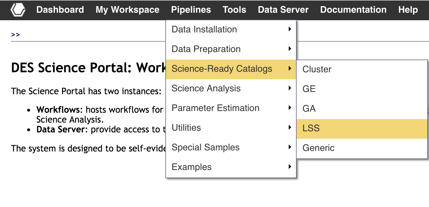
Figure 11: User interface showing the science-ready catalogs menu and the different pipelines available.

As described in Section 3, there are several data products involved in the creation of a science-ready catalog. In addition, we want to support multiple data releases and multiple versions of a given data product with various configurations. This approach sometimes results in hundreds of options. Figure LABEL:fig:input_data shows the user interface designed to simplify the input data selection. The user starts by filtering the available data products by Release and Dataset. In the interface, the result set is grouped by type, in this case, Objects Catalog, Photo-z and Star-galaxy separation. Once the Release and Dataset are selected, there are still many input data options for each product type. For instance, the figure lists the available Photo-$z$s identified by class, related to the Photo-$z$ method used. In order to help further the input data selection, the Process ID, Configuration, Creation Date, Owner and Provenance information are available for each option. Finally, the product types available for selection are pipeline dependent, so data products that are fixed by Data Release and Data Set, (such as the ancillary maps), are internally discovered by the

uery_builder }, simplifying the data selection done by the user.
%
    \begin{figure*}
    \centering
    \includegraphics[width=0.9\textwidth]{input_data}
    \caption{User interface for selecting the input data showing the available photo-$z$s, one of the value-added data products used to create  science-ready catalogs.}
    \label{fig:input_data}
    \end{figure*}
%
The next step is the catalog configuration. Figure~\ref{fig:configuration} shows the configuration interface with General Information about the catalog being created and the configuration parameters for the \textit{region selection}, \textit{object selection} and \textit{column selection} steps. Configurations can be saved, loaded and set as default. There is also a system default configuration that can be restored using the reset button in the configuration manager interface. As a starting point, either the configuration that was set as default (if any) or the system default configuration is presented to the user (see ~\ref{app:

uery_builder). Currently, there are about fifty configuration parameters for the query_builder, showing the importance of having the configuration manager to keep multiple configurations for each pipeline. After the configuration step, a summary table showing the selected options is presented to the user along with a button to submit the process to create the science-ready catalog.

Given the present infrastructure, it is expected that several catalogs with different input data selections and configurations will be created making it very hard to keep track of all of them without a proper tool. That motivated the development of a dashboard, which has been successfully used to monitor the processes and the data products created in the different stages of the portal. In particular, for the Science-ready Catalog stage, it is possible to list all the processes that created catalogs for a given Release, Dataset and pipeline, and from that list access information about the process execution. Examples of accessible information are: process start time and duration, owner, status, if it was saved, shared or published, provenance of the data products used as input, comments made by different users on each process, a detailed process log, the products created by the process and it is also possible to export the products to other instances of the portal. In the current operation model, the export tool is the mechanism used to export the catalogs created at LIneA to the DES Science Database at NCSA.

References

References

- Arnouts et al. [2002] Arnouts, S., Moscardini, L., Vanzella, E., et al., 2002. Measuring the redshift evolution of clustering: the Hubble Deep Field South. MNRAS 329, 355–366. doi:10.1046/j.1365-8711.2002.04988.x, arXiv:astro-ph/0109453.
- Arnouts et al. [2001] Arnouts, S., Vandame, B., Benoist, C., et al., 2001. ESO imaging survey. Deep public survey: Multi-color optical data for the Chandra Deep Field South. A&A 379, 740--754. doi:10.1051/0004-6361:20011341, arXiv:astro-ph/0103071.
- Benoist [2018] Benoist, C., 2018. Wazp Cluster Finder (in preparation).
- Bernyk et al. [2016] Bernyk, M., Croton, D.J., Tonini, C., et al., 2016. The Theoretical Astrophysical Observatory: Cloud-based Mock Galaxy Catalogs. ApJS 223, 9. doi:10.3847/0067-0049/223/1/9, arXiv:1403.5270.