Learning to Transfer

Abstract

Transfer learning borrows knowledge from a source domain to facilitate learning in a target domain. Two primary issues to be addressed in transfer learning are what and how to transfer. For a pair of domains, adopting different transfer learning algorithms results in different knowledge transferred between them. To discover the optimal transfer learning algorithm that maximally improves the learning performance in the target domain, researchers have to exhaustively explore all existing transfer learning algorithms, which is computationally intractable. As a trade-off, a sub-optimal algorithm is selected, which requires considerable expertise in an ad-hoc way. Meanwhile, it is widely accepted in educational psychology that human beings improve transfer learning skills of deciding what to transfer through meta-cognitive reflection on inductive transfer learning practices. Motivated by this, we propose a novel transfer learning framework known as Learning to Transfer (L2T) to automatically determine what and how to transfer are the best by leveraging previous transfer learning experiences. We establish the L2T framework in two stages: 1) we first learn a reflection function encrypting transfer learning skills from experiences; and 2) we infer what and how to transfer for a newly arrived pair of domains by optimizing the reflection function. Extensive experiments demonstrate the L2T’s superiority over several state-of-the-art transfer learning algorithms and its effectiveness on discovering more transferable knowledge.

1 Introduction

Inspired by human beings’ capabilities to transfer knowledge across tasks, transfer learning aims to leverage knowledge from a source domain to improve the learning performance or minimize the number of labeled examples required in a target domain. It is of particular significance when tackling tasks with limited labeled examples. Transfer learning has proved its wide applicability in, such as image classification [15], sentiment classification [4], dialog systems [18] and urban computing [27].

Three key research issues in transfer learning, pointed by Pan and Yang, are when to transfer, how to transfer, and what to transfer. Once transfer learning from a source domain is considered to benefit a target domain (when to transfer), an algorithm (how to transfer) should discover the shared knowledge to be transferred across domains (what to transfer). Different algorithms are likely to discover different parts of transferable knowledge, and thereby lead to uneven transfer learning effectiveness which is evaluated by the performance improvement after transfer learning is conducted. To achieve the optimal performance improvement for a pair of source and target domains, researchers may try tens to hundreds of transfer learning algorithms covering instance [6], parameter [25], and feature [20] based algorithms. This brute-force exploration is computationally expensive and practically impossible. As a tradeoff, a sub-optimal improvement is usually obtained from a heuristically selected algorithm, which unfortunately requires considerable expertise in an ad-hoc and unsystematic manner.

Exploring different algorithms is not the only way to better determine what to transfer and thereby improve transfer learning effectiveness. Previous transfer learning experiences do also help, which has been widely accepted in educational psychology [3, 16]. Human beings sharpen transfer learning skills for deciding what to transfer by conducting meta-cognitive reflection on thorough and diverse transfer learning experiences. For example, children who are good at playing chess may transfer mathematical skills, reading skills, visuospatial skills, and decision making skills learned from chess to solve arithmetic problems, to comprehend reading materials, to solve pattern matching puzzles, and to play basketball, respectively. At a later age, it will be easier for them to decide to transfer mathematical and decision making skills learned from chess, rather than reading and visuospatial skills, to market investment. Unfortunately, all existing transfer learning algorithms transfer from scratch and ignore previous transfer learning experiences.

Motivated by this, we propose a novel transfer learning framework called Learning to Transfer (L2T). The key idea of the L2T framework is to enhance transfer learning effectiveness by leveraging previous transfer learning experiences to automatically determine what and how to transfer are the best for a pair of source and target domains of interest. To achieve the goal, we establish the L2T framework in two stages. During the first stage, we encode each transfer learning experience into three components including a pair of source and target domains, transferred knowledge parameterized as shared latent feature factors (i.e., what to transfer between them), and performance improvement. We learn from all experiences a reflection function which maps a pair of domains and the transferred knowledge between them to the corresponding performance improvement. The reflection function, therefore, is believed to encrypt the transfer learning skills for deciding what and how to transfer. In the second stage, the knowledge to be transferred between a newly arrived pair of domains is optimized so that the value of the learned reflection function, matching to the performance improvement, is maximized.

The contribution of this paper is that we propose a novel transfer learning framework which opens a new door to improve transfer learning effectiveness by taking advantages of previous transfer learning experiences. The L2T can discover more transferable knowledge across domains in a systematic and automatic fashion without requiring considerable expertise, which is also evidenced in comprehensive empirical studies showing the L2T’s superiority over state-of-the-art transfer learning algorithms.

2 Related Work

Transfer Learning

To successfully conduct transfer learning, one of the most critical research issues identified in [19] is to decide what and how to transfer. Parameters [25, 28], instances [6], or latent feature factors [20] can be transferred between domains. A few works [25, 28] transfer parameters from source domains to a target domain as regularizers of SVM-based models. In [6], a basic learner in a target domain is boosted by borrowing the most useful instances from a source domain. Different techniques capable of extracting transferable latent feature factors between domains have been investigated extensively. These techniques include manually selected pivot features [4], dimension reduction [1, 2, 20], collective matrix factorization [14], dictionary learning and sparse coding [21, 31], manifold learning [8, 9], and deep learning [15, 26, 30]. Unlike L2T, all existing studies in transfer learning transfer from scratch, i.e., only considering the source domain and target domain of interest but ignoring previous transfer learning experiences. Since any existing transfer learning algorithm mentioned above could be applied in a transfer learning experience, L2T can even collect all algorithms’ wisdom together.

Lifelong Learning

Assuming a new learning task to lie in the same environment as training tasks, learning to learn [24] or meta-learning [17] transfers knowledge shared among the training tasks to the new task. Ruvolo and Eaton considered lifelong learning as an online meta-learning. Though L2T and lifelong learning both aim to continuously improve a learning system by leveraging histories, L2T differs from them in that each task we consider is a transfer learning task rather than a traditional learning task. Therefore, we learn transfer learning skills instead of task-sharing knowledge.

3 Learning to Transfer

We begin by first introducing the proposed L2T framework. Then we detail the two steps involved in the framework, i.e., learning transfer learning skills from previous transfer learning experiences and applying those skills to infer what and how to transfer for a future pair of source and target domains.

3.1 The L2T Framework

A L2T agent previously conducted transfer learning several times, and kept a record of $N_{e}$ transfer learning experiences (see step (1) in Figure 1). We define each transfer learning experience as $E_{e}=(\mathcal{S}_{e},\mathcal{T}_{e},a_{e},l_{e})$ in which $\mathcal{S}_{e}=\{\mathbf{X}^{s}_{e},\mathbf{y}^{s}_{e}\}$ and $\mathcal{T}_{e}=\{\mathbf{X}^{t}_{e},\mathbf{y}^{t}_{e}\}$ denote a source domain and a target domain, respectively. $\mathbf{X}^{*}_{e}\in\mathbb{R}^{n_{e}^{*}\times m}$ represents the feature matrix if either domain has $n^{*}_{e}$ examples in a $m$-dimensional feature space $\mathcal{X}_{e}^{*}$, where the superscript $*$ can be either $s$ or $t$ to denote a source or target domain. $\mathbf{y}^{*}_{e}\in\mathcal{Y}^{*}_{e}$ denotes the vector of labels with the length being $n_{le}^{*}$. The number of target labeled examples is much smaller than that of source labeled examples, i.e., $n_{le}^{t}\ll n_{le}^{s}$. We focus on the setting $\mathcal{X}_{e}^{s}=\mathcal{X}_{e}^{t}$ and $\mathcal{Y}_{e}^{s}\neq\mathcal{Y}_{e}^{t}$ for each pair of domains. $a_{e}\in\mathcal{A}=\{a_{1},\cdots,a_{N_{a}}\}$ denotes a transfer learning algorithm randomly selected from the set $\mathcal{A}$ containing $N_{a}$ base algorithms. Suppose that what to transfer inferred by the algorithm $a_{e}$ can be parameterized as $\mathbf{W}_{e}$. Finally, each transfer learning experience is labeled with the performance improvement ratio $l_{e}=p^{st}_{e}/p^{t}_{e}$ where $p^{t}_{e}$ is the learning performance (e.g., classification accuracy) in $\mathcal{T}_{e}$ without transfer on a test dataset and $p^{st}_{e}$ is the learning performance in $\mathcal{T}_{e}$ after transferring knowledge from $\mathcal{S}_{e}$ on the same test dataset.

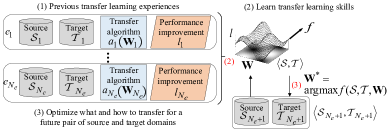
Figure 1: Illustration of the L2T framework.

With all previous transfer learning experiences as the input, the L2T agent aims to learn a function $f$ such that $f(\mathcal{S}_{e},\mathcal{T}_{e},\mathbf{W}_{e})$ approximates $l_{e}$ as shown in step (2) of Figure 1. We call $f$ a reflection function which encrypts the meta-cognitive transfer learning skills - what and how to transfer can maximize the improvement ratio given a pair of source and target domains. Whenever a new pair of domains $\langle\mathcal{S}_{N_{e}+1},\mathcal{T}_{N_{e}+1}\rangle$ arrives, the L2T agent can identify the optimal knowledge to be transferred for this new pair, which is contained in $\mathbf{{W}}^{*}_{N_{e}+1}$, by maximizing $f$ (i.e., step (3) in Figure 1).

3.2 Parameterizing What to Transfer

Adopting different algorithms for one pair of source and target domains brings different what to transfer between them. To learn the reflection function with what to transfer as one input, we have to uniformly parameterize “what to transfer” for all algorithms in the base algorithm set $\mathcal{A}$. In this work, we consider $\mathcal{A}$ to contain algorithms transferring only single-level latent feature factors, because other existing parameter-based and instance-based algorithms cannot address the transfer learning setting we focus on (i.e., $\mathcal{X}^{e}_{s}=\mathcal{X}^{e}_{t}$ and $\mathcal{Y}^{e}_{s}\neq\mathcal{Y}^{e}_{t}$). Though limited parameter-based algorithms [25, 28] can transfer across domains in heterogeneous label spaces, they can only handle binary classification problems. Deep neural network based algorithms [15, 26, 30] transferring latent feature factors in a hierarchy are left for our future research. As a consequence, what to transfer can be parameterized with a latent feature factor matrix $\mathbf{W}$, which we will elaborate in the following.

Latent feature factor based algorithms for the transfer learning setting mentioned above aim to learn domain-invariant feature factors across domains. Consider classifying dog pictures as a source domain and cat pictures as a target domain. The domain-invariant feature factors could include eyes, mouth, tails, etc. Re-characterized with the latent feature factors which are more descriptive, a target domain is expected to achieve better performance with less labeled examples. What to transfer, in this case, is these shared feature factors across domains. According to different ways of extracting the domain-invariant feature factors, existing latent feature factor based algorithms can be categorized into two groups, i.e., common latent space based algorithms and manifold ensemble based algorithms.

Common latent space based algorithms

This line of algorithms, including but not limited to TCA [20], LSDT [31], and DIP [1], assumes that the domain-invariant feature factors lie in a single shared latent space. We denote by $\varphi$ the function mapping the original feature representation into the latent space. If $\varphi$ is linear, it can be represented as an embedding matrix $\mathbf{W}\in\mathbb{R}^{m\times u}$ where $u$ is the dimensionality of the latent space. Therefore, we can parameterize the latent space, what to transfer we focus on, with $\mathbf{W}$ which describes the $u$ latent feature factors. Otherwise, if $\varphi$ is nonlinear, the latent space can still be parameterized with $\mathbf{W}$. Although a nonlinear $\varphi$ is not explicitly specified in most cases such as LSDT using sparse coding, transformed target instances in the latent space $\mathbf{Z}^{t}_{e}=\varphi(\mathbf{X}^{t}_{e})\in\mathbb{R}^{n^{t}_{e}\times u}$ are always available. Consequently, we can infer the similarity metric matrix [5] in the latent space, i.e., $\mathbf{G}\in\mathbb{R}^{m\times m}$, according to $\mathbf{X}^{t}_{e}\mathbf{G}(\mathbf{X}^{t}_{e})^{T}=\mathbf{Z}^{t}_{e}(\mathbf{Z}^{t}_{e})^{T}$. The solution $\mathbf{G}=(\mathbf{X}^{t}_{e})^{\dagger}\mathbf{Z}^{t}_{e}(\mathbf{Z}^{t}_{e})^{T}[(\mathbf{X}^{t}_{e})^{T}]^{\dagger}$ where $(\mathbf{X}^{t}_{e})^{\dagger}$ is the psudo-inverse of $\mathbf{X}^{t}_{e}$. By performing LDL decomposition on $\mathbf{G}=\mathbf{L}\mathbf{D}\mathbf{L}^{T}$, we infer the latent feature factor matrix $\mathbf{W}=\mathbf{L}\mathbf{D}^{1/2}$.

Manifold ensemble based algorithms

Initiated by Gopalan et al., manifold ensemble algorithms consider that a source and a target domain share multiple subspaces (of the same dimension) as points on the Grassmann manifold between them. The representation of a target domain on $u$ domain-invariant latent factors turns to $\mathbf{Z}_{e}^{t(n_{u})}=[\varphi_{1}(\mathbf{X}_{e}^{t}),\cdots,\varphi_{n_{u}}(\mathbf{X}_{e}^{t})]\in\mathbb{R}^{n^{t}_{e}\times n_{u}u}$, if $n_{u}$ subspaces on the manifold are sampled. When all continuous subspaces on the manifold are considered, i.e., $n_{u}\rightarrow\infty$,  Gong et al. proved that $\mathbf{Z}^{t(\infty)}_{e}(\mathbf{Z}^{t(\infty)}_{e})^{T}=\mathbf{X}^{t}_{e}\mathbf{G}(\mathbf{X}^{t}_{e})^{T}$ where $\mathbf{G}$ is the similarity metric matrix. For computational details of $\mathbf{G}$, please refer to [8]. $\mathbf{W}=\mathbf{L}\mathbf{D}^{1/2}$, therefore, is also qualified to represent the latent feature factors distributed in a series of subspaces on a manifold.

3.3 Learning from Experiences

The goal here is to learn a reflection function $f$ such that $f(\mathcal{S}_{e},\mathcal{T}_{e},\mathbf{W}_{e})$ can approximate $l_{e}$ for all experiences $e\in\{1,\cdots,N_{e}\}$. The improvement ratio $l_{e}$ is closely related to two aspects: 1) the difference between a source and a target domain in the shared latent space, and 2) the discriminative ability of a target domain in the latent space. The smaller difference guarantees more overlap between domains in the latent space, which signifies more transferable latent feature factors and higher improvement ratios as a result. The more discriminative ability of a target domain in the latent space is also vital to improve performances. Therefore, we build $f$ to take both aspects into consideration.

The difference between a source and a target domain

We follow [1, 20] and adopt the maximum mean discrepancy (MMD) [11] to measure the difference between a source and a target domain. By mapping two domains into the reproducing kernel Hilbert space (RKHS), MMD empirically evaluates the distance between the means of instances from a source domain and a target domain:

$$\hat{d}_{e}^{2}(\mathbf{X}^{s}_{e}\mathbf{W}_{e},\mathbf{X}^{t}_{e}\mathbf{W}_{e})= \bigg{\|}\frac{1}{n^{s}_{e}}\sum_{i=1}^{n^{s}_{e}}\phi(\mathbf{x}^{s}_{ei}\mathbf{W}_{e})-\frac{1}{n^{t}_{e}}\sum_{j=1}^{n^{t}_{e}}\phi(\mathbf{x}^{t}_{ej}\mathbf{W}_{e})\bigg{\|}_{\mathcal{H}}^{2}=\frac{1}{(n^{s}_{e})^{2}}\sum_{i,i^{\prime}=1}^{n^{s}_{e}}\mathcal{K}(\mathbf{x}^{s}_{ei}\mathbf{W}_{e},\mathbf{x}^{s}_{ei^{\prime}}\mathbf{W}_{e})$$

$$+\frac{1}{(n^{t}_{e})^{2}}\sum_{j,j^{\prime}=1}^{n^{t}_{e}}\mathcal{K}(\mathbf{x}^{t}_{ej}\mathbf{W}_{e},\mathbf{x}^{t}_{ej^{\prime}}\mathbf{W}_{e})-\frac{2}{n^{s}_{e}n^{t}_{e}}\sum_{i,j=1}^{n^{s}_{e},n^{t}_{e}}\mathcal{K}(\mathbf{x}^{s}_{ei}\mathbf{W}_{e},\mathbf{x}^{t}_{ej}\mathbf{W}_{e}),$$ (1)

where $\phi$ maps from the $u$-dimensional latent space to the RKHS $\mathcal{H}$ and $\mathcal{K}(\cdot,\cdot)=\langle\phi(\cdot),\phi(\cdot)\rangle$ is the kernel function. Using different nonlinear mappings $\phi$ (or equivalently different kernels $\mathcal{K}$) leads to different MMD distances and thereby different values of $f$. Therefore, learning the reflection function $f$ is equivalent to finding out the optimal $\phi$ (or $\mathcal{K}$) such that the MMD distance can well characterize the improvement ratio $l_{e}$ for all pairs of domains. Considering the difficulty of directly defining and learning $\phi$, we learn the optimal $\mathcal{K}$ alternatively. Inspired by multiple kernel MMD [11], we parameterize $\mathcal{K}$ as a combination of $N_{k}$ candidate PSD kernels, i.e., $\mathcal{K}=\sum_{k=1}^{N_{k}}\beta_{k}\mathcal{K}_{k}$ where $\beta_{k}\geq 0,\forall k$, and learn the combination coefficients $\boldsymbol{\beta}=[\beta_{1},\cdots,\beta_{N_{k}}]$ instead. As a result, the MMD can be rewritten as $\hat{d}_{e}^{2}(\mathbf{X}^{s}_{e}\mathbf{W}_{e},\mathbf{X}^{t}_{e}\mathbf{W}_{e})=\sum_{k=1}^{N_{k}}\beta_{k}\hat{d}_{e(k)}^{2}(\mathbf{X}^{s}_{e}\mathbf{W}_{e},\mathbf{X}^{t}_{e}\mathbf{W}_{e})=\boldsymbol{\beta}^{T}\mathbf{\hat{d}}_{e}$, where $\mathbf{\hat{d}}_{e}=[\hat{d}_{e(1)}^{2},\cdots,\hat{d}_{e(N_{k})}^{2}]$ with $\hat{d}_{e(k)}^{2}$ computed using the $k$-th kernel $\mathcal{K}_{k}$. In this paper, we consider $N_{k}$ RBF kernels $\mathcal{K}_{k}(\mathbf{a},\mathbf{b})=\text{exp}(-\|\mathbf{a}-\mathbf{b}\|^{2}/\delta_{k})$ with different bandwidths by varying values of $\delta_{k}$.

Unfortunately, the MMD only measuring the distance between the means of domains is insufficient to measure the difference between two domains. The distance variance among all pairs of instances across domains is also required to fully characterize the difference, because a pair of domains with a small MMD but high variance still have a small overlap. According to [11], Equation (1) is actually the empirical estimation of $d_{e}^{2}(\mathbf{X}^{s}_{e}\mathbf{W}_{e},\mathbf{X}^{t}_{e}\mathbf{W}_{e})=\mathbf{E}_{\mathbf{x}^{s}_{e}\mathbf{x}^{s\prime}_{e}\mathbf{x}^{t}_{e}\mathbf{x}^{t\prime}_{e}}h(\mathbf{x}^{s}_{e},\mathbf{x}^{s\prime}_{e},\mathbf{x}^{t}_{e},\mathbf{x}^{t\prime}_{e})$ where $h(\mathbf{x}^{s}_{e},\mathbf{x}^{s\prime}_{e},\mathbf{x}^{t}_{e},\mathbf{x}^{t\prime}_{e})=\mathcal{K}(\mathbf{x}^{s}_{e}\mathbf{W}_{e},\mathbf{x}^{s\prime}_{e}\mathbf{W}_{e})+\mathcal{K}(\mathbf{x}^{t}_{e}\mathbf{W}_{e},\mathbf{x}^{t\prime}_{e}\mathbf{W}_{e})-\mathcal{K}(\mathbf{x}^{s}_{e}\mathbf{W}_{e},\mathbf{x}^{t\prime}_{e}\mathbf{W}_{e})-\mathcal{K}(\mathbf{x}^{s\prime}_{e}\mathbf{W}_{e},\mathbf{x}^{t}_{e}\mathbf{W}_{e})$. Consequently, the distance variance, $\sigma_{e}^{2}$, equals

$$\sigma_{e}^{2}(\mathbf{X}^{s}_{e}\mathbf{W}_{e},\mathbf{X}^{t}_{e}\mathbf{W}_{e})=\mathbf{E}_{\mathbf{x}^{s}_{e}\mathbf{x}^{s\prime}_{e}\mathbf{x}^{t}_{e}\mathbf{x}^{t\prime}_{e}}\left[\left(h(\mathbf{x}^{s}_{e},\mathbf{x}^{s\prime}_{e},\mathbf{x}^{t}_{e},\mathbf{x}^{t\prime}_{e})-\mathbf{E}_{\mathbf{x}^{s}_{e}\mathbf{x}^{s\prime}_{e}\mathbf{x}^{t}_{e}\mathbf{x}^{t\prime}_{e}}h(\mathbf{x}^{s}_{e},\mathbf{x}^{s\prime}_{e},\mathbf{x}^{t}_{e},\mathbf{x}^{t\prime}_{e})\right)^{2}\right].$$

To be consistent with the MMD characterized with $N_{k}$ candidate kernels, we can also rewrite $\sigma_{e}^{2}=\boldsymbol{\beta}^{T}\mathbf{Q}_{e}\boldsymbol{\beta}$ where $\mathbf{Q}_{e}=\text{cov}(h)=\begin{bmatrix}\sigma_{e(1,1)}&\cdots&\sigma_{e(1,N_{k})}\\ \cdots&\cdots&\cdots\\ \sigma_{e(N_{k},1)}&\cdots&\sigma_{e(N_{k},N_{k})}\end{bmatrix}$. Each element $\sigma_{e(k_{1},k_{2})}=\text{cov}(h_{k_{1}},h_{k_{2}})=\mathbf{E}\left[(h_{k_{1}}-\mathbf{E}h_{k_{1}})(h_{k_{2}}-\mathbf{E}h_{k_{2}})\right]$. Note that $\mathbf{E}h_{k_{1}}$ is shorthand for $\mathbf{E}_{\mathbf{x}^{s}_{e}\mathbf{x}^{s\prime}_{e}\mathbf{x}^{t}_{e}\mathbf{x}^{t\prime}_{e}}h_{k1}(\mathbf{x}^{s}_{e},\mathbf{x}^{s\prime}_{e},\mathbf{x}^{t}_{e},\mathbf{x}^{t\prime}_{e})$ where $h_{k_{1}}$ is calculated using the $k_{1}$-th kernel. Due to unknown data distributions of either source or target domains, we empirically estimate $\mathbf{Q}_{e}$ to be $\mathbf{\hat{Q}}_{e}$ which is detailed in the supplementary material due to page limit.

The discriminative ability of a target domain

Considering the lack of labeled data in a target domain, we resort to unlabeled data to evaluate the discriminative ability instead of using labelled data as usual. The principles of the unlabeled discriminant criterion are two-fold: 1) similar instances should also be neighbours after being embedded into the latent space; and 2) dissimilar instances should be far away. We adopt the unlabeled discriminant criterion proposed in [29],

$$\tau_{e}=\text{tr}(\mathbf{W}_{e}^{T}\mathbf{S}_{e}^{N}\mathbf{W}_{e})/\text{tr}(\mathbf{W}_{e}^{T}\mathbf{S}_{e}^{L}\mathbf{W}_{e}),$$

where $\mathbf{S}_{e}^{L}=\sum_{j,j^{\prime}=1}^{n^{t}_{e}}\frac{H_{jj^{\prime}}}{(n^{t}_{e})^{2}}(\mathbf{x}^{t}_{ej}-\mathbf{x}^{t}_{ej^{\prime}})(\mathbf{x}^{t}_{ej}-\mathbf{x}^{t}_{ej^{\prime}})^{T}$ is the local scatter covariance matrix with the neighbour information $H_{jj^{\prime}}$ defined as $H_{jj^{\prime}}=\begin{cases}\mathcal{K}(\mathbf{x}_{ej}^{t},\mathbf{x}_{ej^{\prime}}^{t}),&\text{if}\quad\mathbf{x}^{t}_{ej}\in\mathcal{N}_{r}(\mathbf{x}^{t}_{ej^{\prime}})\quad\text{and}\quad\mathbf{x}^{t}_{ej^{\prime}}\in\mathcal{N}_{r}(\mathbf{x}^{t}_{ej})\\ 0,&\text{otherwise}\end{cases}$. $\mathbf{x}_{ej}^{t}$ is the $j$-th instance in $\mathbf{X}_{e}^{t}$, and $\text{tr}(\cdot)$ denotes the trace of a square matrix. If $\mathbf{x}^{t}_{ej}$ and $\mathbf{x}^{t}_{ej^{\prime}}$ are mutual $r$-nearest neighbours to each other, the value of $H_{jj^{\prime}}$ equals that of the kernel function $\mathcal{K}(\cdot,\cdot)$. By maximizing the unlabeled discriminant criterion $\tau_{e}$, the local scatter covariance matrix guarantees the first principle, while $\mathbf{S}_{e}^{N}=\sum_{j,j^{\prime}=1}^{n^{t}_{e}}\frac{\mathcal{K}(\mathbf{x}^{t}_{ej},\mathbf{x}^{t}_{ej^{\prime}})-H_{jj^{\prime}}}{(n^{t}_{e})^{2}}(\mathbf{x}^{t}_{ej}-\mathbf{x}^{t}_{ej^{\prime}})(\mathbf{x}^{t}_{ej}-\mathbf{x}^{t}_{ej^{\prime}})^{T}$, the non-local scatter covariance matrix, enforces the second principle. $\tau_{e}$ also depends on the kernel used, since different kernels indicate different neighbour information and different degrees of similarity between neighboured instances. With $\tau_{e(k)}$ obtained from the $k$-th kernel $\mathcal{K}_{k}$, the unlabeled discriminant criterion $\tau_{e}$ can be written as $\tau_{e}=\sum_{k=1}^{N_{k}}\beta_{k}\tau_{e(k)}=\boldsymbol{\beta}^{T}\boldsymbol{\tau}_{e}$ where $\boldsymbol{\tau}_{e}=[\tau_{e(1)},\cdots,\tau_{e(N_{k})}]$.

The optimization problem

Combining the two aspects abovementioned to model the reflection function $f$, we finally formulate the optimization problem as follows,

$$\boldsymbol{\beta}^{*},\lambda^{*},\mu^{*},b^{*}=\arg\min_{\boldsymbol{\beta},\lambda,\mu,b} \ \sum_{e=1}^{N_{e}}\mathcal{L}_{h}\left(\boldsymbol{\beta}^{T}\mathbf{\hat{d}}_{e}+\lambda\boldsymbol{\beta}^{T}\mathbf{\hat{Q}}_{e}\boldsymbol{\beta}+\frac{\mu}{\boldsymbol{\beta}^{T}\boldsymbol{\tau}_{e}}+b,\frac{1}{l_{e}}\right)+\gamma_{1}R(\boldsymbol{\beta},\lambda,\mu,b),$$

s.t. $$\quad\beta_{k}\geq 0,\ \forall k\in\{1,\cdots,N_{k}\},\ \lambda\geq 0,\ \mu\geq 0,$$ (2)

where $1/f=\boldsymbol{\beta}^{T}\mathbf{\hat{d}}_{e}+\lambda\boldsymbol{\beta}^{T}\mathbf{\hat{Q}}_{e}\boldsymbol{\beta}+\frac{\mu}{\boldsymbol{\beta}^{T}\boldsymbol{\tau}_{e}}+b$ and $\mathcal{L}_{h}(\cdot)$ is the Huber regression loss [13] constraining the value of $f$ to be as close to $1/l_{e}$ as possible. $\gamma_{1}$ controls the complexity of the parameters. Minimizing the difference between domains, including the MMD $\boldsymbol{\beta}^{T}\mathbf{\hat{d}}_{e}$ and the distance variance $\boldsymbol{\beta}^{T}\mathbf{\hat{Q}}_{e}\boldsymbol{\beta}$, and meanwhile maximizing the discriminant criterion $\boldsymbol{\beta}^{T}\boldsymbol{\tau}_{e}$ in the target domain will contribute a large performance improvement ratio $l_{e}$ (i.e., a small $1/l_{e}$). $\lambda$ and $\mu$ balance the importance of the three terms in $f$, and $b$ is the bias term.

3.4 Inferring What to Transfer

Once the L2T agent has learned the reflection function $f(\mathcal{S},\mathcal{T},\mathbf{W};\boldsymbol{\beta}^{*},\lambda^{*},\mu^{*},b^{*})$, it can take advantage of the function to infer the optimal what to transfer, i.e., the latent feature factor matrix $\mathbf{W}$, for a newly arrived pair of source domain $\mathcal{S}_{N_{e}+1}$ and target domain $\mathcal{T}_{N_{e}+1}$. The optimal latent feature factor matrix $\mathbf{W}^{*}$ should maximize the value of $f$. To this end, we optimize the following objective with regard to $\mathbf{W}$,

$$\mathbf{W}^{*} =\arg\max_{\mathbf{W}}\ f(\mathcal{S}_{N_{e}+1},\mathcal{T}_{N_{e}+1},\mathbf{W};\boldsymbol{\beta}^{*},\lambda^{*},\mu^{*},b^{*})+\gamma_{2}\|\mathbf{W}\|^{2}_{F}$$

$$=\arg\min_{\mathbf{W}}\ (\boldsymbol{\beta}^{*})^{T}\mathbf{\hat{d}}_{\mathbf{W}}+\lambda^{*}(\boldsymbol{\beta}^{*})^{T}\mathbf{\hat{Q}}_{\mathbf{W}}\boldsymbol{\beta}^{*}+\mu^{*}\frac{1}{(\boldsymbol{\beta}^{*})^{T}\mathbf{\boldsymbol{\tau}}_{\mathbf{W}}}+\gamma_{2}\|\mathbf{W}\|^{2}_{F},$$ (3)

where $\|\cdot\|_{F}$ denotes the matrix Frobenius norm and $\gamma_{2}$ controls the complexity of $\mathbf{W}$. The first and second terms in problem (3) can be calculated as

$$(\boldsymbol{\beta}^{*})^{T}\mathbf{\hat{d}}_{\mathbf{W}}=\sum_{k=1}^{N_{k}}\beta_{k}^{*}\biggl{[}\frac{1}{(n^{s})^{2}}\sum_{i,i^{\prime}=1}^{n^{s}}\mathcal{K}_{k}(\mathbf{x}^{s}_{i}\mathbf{W},\mathbf{x}^{s}_{i^{\prime}}\mathbf{W})+\frac{1}{(n^{t})^{2}}\sum_{j,j^{\prime}=1}^{n^{t}}\mathcal{K}_{k}(\mathbf{x}^{t}_{j}\mathbf{W},\mathbf{x}^{t}_{j^{\prime}}\mathbf{W})-\frac{2}{n^{s}n^{t}}\sum_{i,j=1}^{n^{s},n^{t}}\mathcal{K}_{k}(\mathbf{x}^{s}_{i}\mathbf{W},\mathbf{x}^{t}_{j}\mathbf{W})\biggr{]},$$

$$(\boldsymbol{\beta}^{*})^{T}\mathbf{\hat{Q}}_{\mathbf{W}}\boldsymbol{\beta}^{*}= \frac{1}{n^{2}-1}\sum_{i,i^{\prime}=1}^{n}\sum_{k=1}^{N_{k}}\biggl{\{}\beta^{*}_{k}\biggl{[}\mathcal{K}_{k}(\mathbf{x}^{s}_{i}\mathbf{W},\mathbf{x}^{s}_{i^{\prime}}\mathbf{W})+\mathcal{K}_{k}(\mathbf{x}^{t}_{i}\mathbf{W},\mathbf{x}^{t}_{i^{\prime}}\mathbf{W})-2\mathcal{K}_{k}(\mathbf{x}^{s}_{i}\mathbf{W},\mathbf{x}^{t}_{i^{\prime}}\mathbf{W})$$

$$-\frac{1}{n^{2}}\sum_{i,i^{\prime}=1}^{n}\biggl{(}\mathcal{K}_{k}(\mathbf{x}^{s}_{i}\mathbf{W},\mathbf{x}^{s}_{i^{\prime}}\mathbf{W})+\mathcal{K}_{k}(\mathbf{x}^{t}_{i}\mathbf{W},\mathbf{x}^{t}_{i^{\prime}}\mathbf{W})-2\mathcal{K}_{k}(\mathbf{x}^{s}_{i}\mathbf{W},\mathbf{x}^{t}_{i^{\prime}}\mathbf{W})\biggr{)}\biggr{]}\biggr{\}}^{2},$$

where $n=\min(n^{s},n^{t})$. The third term in problem (3) can be computed as $(\boldsymbol{\beta}^{*})^{T}\boldsymbol{\tau}_{\mathbf{W}}=\sum_{k=1}^{N_{k}}\beta^{*}_{k}\frac{\text{tr}(\mathbf{W}^{T}\mathbf{S}^{N}_{k}\mathbf{W})}{\text{tr}(\mathbf{W}^{T}\mathbf{S}^{L}_{k}\mathbf{W})}$. We optimize the non-convex problem (3) w.r.t $\mathbf{W}$ by employing a conjugate gradient method in which the gradient is listed in the supplementary material due to page limit.

4 Experiments

In this section, we empirically test the performance of the proposed L2T framework.

Datasets

We evaluate the L2T framework on two image datasets, Caltech-256 [12] and Sketches [7]. Caltech-256, collected from Google Images, contains a total of 30,607 images in 256 categories. The Sketches dataset, however, consists of 20,000 unique sketches by human beings that are evenly distributed over 250 different categories. There is an overlap between the 256 categories in Caltech-256 and the 250 categories in Sketches, e.g., “backpack” and “horse”. Obviously, the Caltech-256 images lie in a different distribution from the Sketches, so that we can regard one of them as the source domain and the other as the target domain. We construct each pair of source and target domains by randomly sampling three categories from Caltech-256 as the source domain and randomly sampling three categories from Sketches as the target domain, which we give an example in the supplementary material. Consequently, there are $20,000/250\times 3=720$ examples in the target domain of each pair. In total, we generate 1,000 training pairs for transfer learning experiences, 500 validation pairs to determine hyperparameters of the reflection function, and 500 testing pairs to evaluate the reflection function. We characterize each image from both datasets using 4,096-dimensional features extracted by a convolutional neural network pre-trained by the ImageNet dataset.

Baselines and Evaluation Metrics

We compare the proposed L2T framework with the following nine baseline algorithms, including one without transfer learning and the other eight feature-based transfer learning algorithms in two categories, i.e., common latent space and manifold ensemble. The Original builds a model using labeled data in the target domain only. The common latent space based algorithms are listed as follows. The TCA [20] learns transferable components across domains on which the embeddings of two domains have the minimum MMD. The ITL [23] learns a common subspace where instances from both domains are distributed not only similarly but also discriminatively via optimizing an information-theoretic metric. The graph co-regularized matrix factorization proposed in [14], denoted as CMF, extracts a common subspace in which geometric structures within each domain and across domains are preserved. The LSDT [31] learns a common subspace where instances in a target domain can be sparsely reconstructed by the combined source and target instances. The self-taught learning (STL) [21] learns a dictionary from a source domain and obtains enriched representations of target instances based on the learned dictionary. The DIP [1] and SIE [2] learn a domain-invariant projection which can minimize the MMD and the Hellinger distance between domains, respectively. The GFK [8], a manifold ensemble based algorithm, embeds a source and a target domain onto a Grassmann manifold and projections in an infinite number of subspaces along the manifold are integrated to represent the target domain. The eight feature-based transfer learning algorithms are also the base transfer learning algorithms used to generate experiences in Section 3.2. Based on feature representations obtained by different algorithms, we use the nearest-neighbor classifier to perform three-class classification for the target domain.

We use the classification accuracy on the test data of the target domain as an evaluation metric. Since target domains are at different levels of difficulty, accuracies are incomparable for different pairs of domains. To evaluate the L2T on different pairs of source and target domains, we adopt the performance improvement ratio defined in Section 3.1 as another evaluation metric.

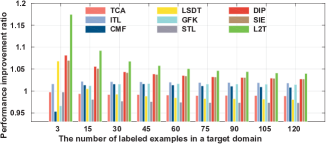
Figure 2: Average performance improvement ratio comparison over 500 testing pairs of source and target domains.

Performance Comparison

In this experiment, we learn a reflection function from 1,000 transfer learning experiences, and evaluate the reflection function on 500 testing pairs of source and target domains by comparing the average performance improvement ratio with the baselines. In building the reflection function, we use $33$ RBF kernels with the bandwidth $\delta_{k}$ in the range of $[2^{-8}\eta:2^{0.5}\eta:2^{8}\eta]$ where $\eta=\frac{1}{n^{s}n^{t}}\sum_{i,j=1}^{n^{s},n^{t}}\|\mathbf{x}^{s}_{i}\mathbf{W}-\mathbf{x}^{t}_{j}\mathbf{W}\|^{2}_{2}$ following the median trick [10]. As Figure 2 shows, on average the proposed L2T framework outperforms the baselines up to $10\%$ when varying the number of labeled samples in the target domain. As the number of labeled examples in a target domain used for building the classifier increases from 3 to 120, the performance improvement ratio becomes smaller because the classification accuracy without transfer tends to increase. The baseline algorithms behave differently. The transferable knowledge learned by LSDT helps a target domain a lot when training examples are scarce, while GFK performs poorly until training examples become more. STL is almost the worst baseline because it learns a dictionary from the source domain only but ignores the target domain. It runs at a high risk of failure especially when two domains are distant. DIP and SIE, which minimize the MMD and Hellinger distance between domains subject to manifold constraints, are competent. Note that we have run the paired $t$-test between L2T and each baseline with all the $p$-values on the order of $10^{-12}$, concluding that the L2T is significantly superior.

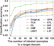
(a) galaxy / harpsichord / saturn
$\rightarrow$ kangaroo / standing-bird / sun

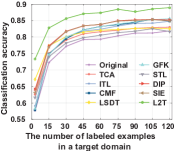
(b) bat / mountain-bike / saddle
$\rightarrow$ bush / person / walkie-talkie

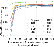
(c) microwave / spider / watch
$\rightarrow$ spoon / trumpet / wheel

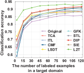
(d) bridge / harp / traffic-light
$\rightarrow$ door-handle / hand / present

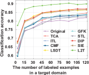
(e) bridge / helicopter / tripod
$\rightarrow$ key / parrot / traffic-light

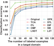
(f) caculator / straw / french-horn
$\rightarrow$ doorknob / palm-tree / scissors

Figure 3: Classification accuracies on six pairs of source and target domains.

We also randomly select six of the 500 testing pairs and compare classification accuracies by different algorithms for each pair in Figure 3. The performance of all baselines varies from pair to pair. Among all the baseline methods, TCA performs the best when transferring between domains in Figure 3(a) and LSDT is the most superior in Figure 3(c). However, L2T consistently outperforms the baselines on all the settings. For some pairs, e.g., Figures 3(a), 3(c) and 3(f), the three classes in the target domains are comparably easy to tell apart, hence the Original without transfer can achieve even better results than some transfer learning algorithms. In this case, L2T still improves by discovering the best transferable knowledge from the source domain, especially when the number of labeled examples is small (see Figure 3(c) and 3(f)). If two domains are very related, e.g., the source with “galaxy” and “saturn” and the target with “sun” in Figure 3(a), L2T even finds out more transferable knowledge and contributes more significant improvement.

Table 1: The performance improvement ratios by varying different approaches used to generate transfer learning experiences. For example, “ITL+L2T” denotes the L2T learning from experiences generated by ITL only, and the second line of results for “ITL+L2T” is the $p$-value compared to ITL.

# of labeled examples 3 15 30 45 60 75 90 105 120 TCA 1.0181 1.0024 0.9965 0.9973 0.9941 0.9933 0.9938 0.9927 0.9928 ITL 1.0188 1.0248 1.0250 1.0254 1.0250 1.0224 1.0232 1.0224 1.0224 CMF 0.9607 1.0203 1.0224 1.0218 1.0190 1.0158 1.0144 1.0142 1.0125 LSDT 1.0828 1.0168 0.9988 0.9940 0.9895 0.9867 0.9854 0.9834 0.9837 GFK 0.9729 1.0180 1.0232 1.0243 1.0246 1.0219 1.0239 1.0229 1.0225 STL 0.9973 0.9771 0.9715 0.9713 0.9715 0.9694 0.9705 0.9693 0.9693 DIP 1.0875 1.0633 1.0518 1.0465 1.0425 1.0372 1.0365 1.0343 1.0317 SIE 1.0745 1.0579 1.0485 1.0448 1.0412 1.0359 1.0359 1.0334 1.0318 ITL + L2T 1.1210 1.0737 1.0577 1.0506 1.0456 1.0398 1.0394 1.0361 1.0359 0.0000 0.0000 0.0000 0.0000 0.0000 0.0000 0.0000 0.0002 0.0002 DIP + L2T 1.1605 1.0927 1.0718 1.0620 1.0562 1.0500 1.0483 1.0461 1.0451 [t] 0.0000 0.0000 0.0000 0.0000 0.0000 0.0000 0.0000 0.0000 0.0000 (LSDT/GFK /SIE) + L2T 1.1660 1.0973 1.0746 1.0652 1.0573 1.0506 1.0485 1.0451 1.0429 [t] 0.0000 0.0000 0.0000 0.0000 0.0000 0.0000 0.0000 0.0000 0.0000 (TCA/ITL/CMF/GFK /LSDT/SIE/) + L2T 1.1712 1.0954 1.0707 1.0607 1.0529 1.0469 1.0449 1.0421 1.0416 [t] 0.0000 0.0000 0.0001 0.0001 0.0106 0.0019 0.0002 0.0047 0.0106 [t] all + L2T 1.1872 1.1054 1.0795 1.0699 1.0616 1.0551 1.0531 1.0500 1.0502

Varying the Experiences

We further investigate how transfer learning experiences used to learn the reflection function influence the performance of L2T. In this experiment, we evaluate on 50 randomly sampled pairs out of the 500 testing pairs in order to efficiently investigate a wide range of cases in the following. The sampled set is unbiased and sufficient to characterize such influence, evidenced by the asymptotic consistency of the average performance improvement ratio on the 500 pairs in Figure 2 and the 50 pairs in the last line of Table 1. First, we fix the number of transfer learning experiences to be 1,000 and vary the set of base transfer learning algorithms. The results are shown in Table 1. Even with experiences generated by single base algorithm, e.g., ITL or DIP, the L2T can still learn a reflection function that significantly better ($p$-value < 0.05) decides what to transfer than using ITL or DIP directly. With more base algorithms involved, the transfer learning experiences are more informative to cover more situations of source-target pairs and the knowledge transferred between them. As a result, the L2T learns a better reflection function and thereby achieves higher performance improvement ratios. Second, we fix the set of base algorithms to include all the eight baselines and vary the number of transfer learning experiences used for training. As shown in Figure 6, the average performance improvement ratio achieved by L2T tends to increase as the number of labeled examples in the target domain decreases, and more importantly it increases as the number of experiences increases. This lays the foundation for further conducting L2T in an online manner which can gradually assimilate transfer learning experiences and continuously improve.

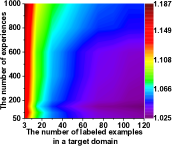
Figure 4: Varying the number of transfer learning experiences.

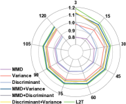
Figure 5: Varying the components constituted in the $f$.

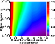
Figure 6: Varying the number of kernels considered in the $f$.

Varying the Reflection Function

We also study the influence of different configurations of the reflection function on the performance of L2T. First, we vary the components to be considered in building the reflection function $f$ as shown in Figure 6. Considering single type, either MMD, variance, or the discriminant criterion, brings inferior performance and even negative transfer. L2T taking all the three factors into consideration outperforms the others, demonstrating that the three components are all necessary and mutually reinforcing. With all the three components included, we plot values of the learned $\boldsymbol{\beta}^{*}$ in the supplementary material. Second, we change different kernels used. In Figure 6, we present results by either narrowing down or extending the range $[2^{-8}\eta:2^{0.5}\eta:2^{8}\eta]$. Obviously, more kernels (e.g., $[2^{-12}\eta:2^{0.5}\eta:2^{12}\eta]$), capable of encrypting better transfer learning skills in the reflection function, achieve larger performance improvement ratios.

5 Conclusion

In this paper, we propose a novel L2T framework for transfer learning which automatically determines what and how to transfer is the best between a source and a target domain by leveraging previous transfer learning experiences. In particular, L2T learns a reflection function mapping a pair of domains and the knowledge transferred between them to the performance improvement ratio. When a new pair of domains arrives, L2T optimizes what and how to transfer by maximizing the value of the learned reflection function. We believe that L2T opens a new door to improve transfer learning by leveraging transfer learning experiences. Many research issues, e.g., incorporating hierarchical latent feature factors as what to transfer and designing online L2T, can be further investigated.

 

Learning to Transfer: Supplementary Material

 

1 Empirical Estimation of $\mathbf{Q}_{e}$

$$\mathbf{\hat{Q}}_{e}= \frac{1}{n^{2}-1}\sum_{i,i^{\prime}=1}^{n}\sum_{k=1}^{N_{k}}\biggl{[}\mathcal{K}_{k}(\mathbf{x}^{s}_{i}\mathbf{W},\mathbf{x}^{s}_{i^{\prime}}\mathbf{W})+\mathcal{K}_{k}(\mathbf{x}^{t}_{i}\mathbf{W},\mathbf{x}^{t}_{i^{\prime}}\mathbf{W})-2\mathcal{K}_{k}(\mathbf{x}^{s}_{i}\mathbf{W},\mathbf{x}^{t}_{i^{\prime}}\mathbf{W})$$

$$-\frac{1}{n^{2}}\sum_{i,i^{\prime}=1}^{n}\biggl{(}\mathcal{K}_{k}(\mathbf{x}^{s}_{i}\mathbf{W},\mathbf{x}^{s}_{i^{\prime}}\mathbf{W})+\mathcal{K}_{k}(\mathbf{x}^{t}_{i}\mathbf{W},\mathbf{x}^{t}_{i^{\prime}}\mathbf{W})-2\mathcal{K}_{k}(\mathbf{x}^{s}_{i}\mathbf{W},\mathbf{x}^{t}_{i^{\prime}}\mathbf{W})\biggr{)}\biggr{]}^{2},$$ (4)

where $n=\min(n^{s}_{e},n^{t}_{e})$.

2 The Gradient towards Optimizing $\mathbf{W}$

$$\frac{\partial\mathcal{L}}{\partial\mathbf{W}}=\frac{\partial(\boldsymbol{\beta}^{*})^{T}\mathbf{\hat{d}}_{\mathbf{W}}}{\partial\mathbf{W}}+\lambda^{*}\frac{\partial(\boldsymbol{\beta}^{*})^{T}\mathbf{\hat{Q}}_{\mathbf{W}}\boldsymbol{\beta}^{*}}{\partial\mathbf{W}}-\mu^{*}\frac{1}{[(\boldsymbol{\beta}^{*})^{T}\boldsymbol{\tau}_{\mathbf{W}}]^{2}}\frac{\partial(\boldsymbol{\beta}^{*})^{T}\boldsymbol{\tau}_{\mathbf{W}}}{\partial\mathbf{W}}+2\gamma_{2}\mathbf{W},$$ (5)

among which

$$\frac{\partial(\boldsymbol{\beta}^{*})^{T}\mathbf{\hat{d}}_{\mathbf{W}}}{\partial\mathbf{W}}=\sum_{k=1}^{N_{k}}\beta_{k}^{*}\bigg{[}\frac{1}{(n^{s})^{2}}\sum_{i,i^{\prime}=1}^{n_{s}}\hat{\mathbf{K}}_{k(i,i^{\prime})}^{ss}+\frac{1}{(n^{t})^{2}}\sum_{j,j^{\prime}=1}^{n_{t}}\hat{\mathbf{K}}_{k(j,j^{\prime})}^{tt}-\frac{2}{n^{s}n^{t}}\sum_{i,j=1}^{n_{s},n_{t}}\hat{\mathbf{K}}_{k(i,j)}^{st})\bigg{]},$$ (6)

$$\frac{\partial(\boldsymbol{\beta}^{*})^{T}\mathbf{\hat{Q}}_{\mathbf{W}}\boldsymbol{\beta}^{*}}{\partial\mathbf{W}} =\frac{1}{n^{2}-1}\sum_{k=1}^{N_{k}}\sum_{i,i^{\prime}=1}^{n}\hat{\mathbf{B}}_{k(i,i^{\prime})}\bigg{[}\hat{\mathbf{K}}_{k(i,i^{\prime})}^{ss}+\hat{\mathbf{K}}_{k(i,i^{\prime})}^{tt}-2\hat{\mathbf{K}}_{k(i,i^{\prime})}^{st})$$

$$-\sum_{i,i^{\prime}=1}^{n}\bigg{(}\hat{\mathbf{K}}_{k(i,i^{\prime})}^{ss}+\hat{\mathbf{K}}_{k(i,i^{\prime})}^{tt}-2\hat{\mathbf{K}}_{k(i,i^{\prime})}^{st})\bigg{)}\bigg{]}$$ (7)

$$\frac{\partial(\boldsymbol{\beta}^{*})^{T}\boldsymbol{\tau}_{\mathbf{W}}}{\partial\mathbf{W}}=\sum_{k=1}^{N_{k}}\beta_{k}\frac{2[\text{tr}(\mathbf{W}^{T}\mathbf{S}^{L}_{k}\mathbf{W})]\mathbf{S}^{N}_{k}-2[\text{tr}(\mathbf{W}^{T}\mathbf{S}^{N}_{k}\mathbf{W})]\mathbf{S}^{L}_{k}}{[\text{tr}(\mathbf{W}^{T}\mathbf{S}^{L}_{k}\mathbf{W})]^{2}},$$ (8)

where $\hat{\mathbf{K}}^{ss}_{k(i,i^{\prime})}$, $\hat{\mathbf{K}}^{tt}_{k(j,j^{\prime})}$, and $\hat{\mathbf{K}}^{st}_{k(i,j)}$ depending on the kernel function are calculated as follows,

$$\hat{\mathbf{K}}^{ss}_{k(i,i^{\prime})}=-\frac{2}{\delta_{k}}\mathcal{K}_{k}(\mathbf{x}^{s}_{i}\mathbf{W},\mathbf{x}^{s}_{i^{\prime}}\mathbf{W})(\mathbf{x}^{s}_{i}-\mathbf{x}^{s}_{i^{\prime}})(\mathbf{x}^{s}_{i}-\mathbf{x}^{s}_{i^{\prime}})^{T}\mathbf{W},$$ (9)

$$\hat{\mathbf{K}}^{tt}_{k(i,i^{\prime})}=-\frac{2}{\delta_{k}}\mathcal{K}_{k}(\mathbf{x}^{t}_{i}\mathbf{W},\mathbf{x}^{t}_{i^{\prime}}\mathbf{W})(\mathbf{x}^{t}_{i}-\mathbf{x}^{t}_{i^{\prime}})(\mathbf{x}^{s}_{i}-\mathbf{x}^{s}_{i^{\prime}})^{T}\mathbf{W},$$ (10)

$$\hat{\mathbf{K}}^{st}_{k(i,i^{\prime})}=-\frac{2}{\delta_{k}}\mathcal{K}_{k}(\mathbf{x}^{s}_{i}\mathbf{W},\mathbf{x}^{s}_{i^{\prime}}\mathbf{W})(\mathbf{x}^{s}_{i}-\mathbf{x}^{t}_{i^{\prime}})(\mathbf{x}^{s}_{i}-\mathbf{x}^{t}_{i^{\prime}})^{T}\mathbf{W}.$$ (11)

In Eqaution 7,

$$\hat{\mathbf{B}}_{k(i,i^{\prime})} =\sum_{k=1}^{N_{k}}\sum_{i,i^{\prime}=1}^{n}2\beta^{*}_{k}\bigg{[}\mathcal{K}_{k}(\mathbf{x}^{s}_{i}\mathbf{W},\mathbf{x}^{s}_{i^{\prime}}\mathbf{W})+\mathcal{K}_{k}(\mathbf{x}^{t}_{i}\mathbf{W},\mathbf{x}^{t}_{i^{\prime}}\mathbf{W})-2\mathcal{K}_{k}(\mathbf{x}^{s}_{i}\mathbf{W},\mathbf{x}^{t}_{i^{\prime}}\mathbf{W})$$

$$-\frac{1}{n^{2}}\sum_{i,i^{\prime}=1}^{n}(\mathcal{K}_{k}(\mathbf{x}^{s}_{i}\mathbf{W},\mathbf{x}^{s}_{i^{\prime}}\mathbf{W})+\mathcal{K}_{k}(\mathbf{x}^{t}_{i}\mathbf{W},\mathbf{x}^{t}_{i^{\prime}}\mathbf{W})-2\mathcal{K}_{k}(\mathbf{x}^{s}_{i}\mathbf{W},\mathbf{x}^{t}_{i^{\prime}}\mathbf{W}))\bigg{]}.$$ (12)

3 Exemplar of A Pair of Source and Target Domains

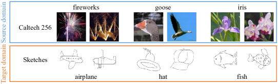
Figure 7: One example pair of source and target domains.

4 Coefficients of RBF Kernels

We plot the values of the coefficients for $N_{k}$ RBF kernels, i.e., $\beta_{k}$ for $k=\{1,\cdots,N_{k}\}$ in Figure 8. Note that we use 33 RBF kernels as stated in the paper.

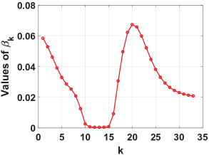
Figure 8: Values of the coefficients for all $N_{k}$ RBF kernels.

5 Discussion on $l_{e}$ in Equation (2)

$l_{e}$, the performance improvement ratio, heavily depends on the number of labeled examples in the target domain $\mathcal{T}_{e}$, i.e., $n^{t}_{le}$. A smaller number of target labeled examples tends to produce a larger performance improvement ratio, and vice versa. Since the $n^{t}_{le}$ varies from experience to experience, we adopt a transformed $\hat{l}_{e}$ instead of $l_{e}$ to train the reflection function in Equation (2). The $\hat{l}_{e}$ is expected to be the expectation of the performance improvement ratio in the range of $[p,q]$ for the $e$-th experience, where $p$ and $q$ are the minimum and maximum number of target labeled examples. To compute the expectation, we first assume that the performance improvement ratio with regard to the number of target labeled examples follows the following monotonically decreasing function,

$$f(x)=\frac{x}{a_{e}+bx},$$ (13)

where $a_{e}$ and $b$ are two parameters deciding the function. $a_{e}$ is conditioned on a specific experience but $b$ is shared across all experiences. Note that $f(n^{t}_{le})=l_{e}$. As a consequence, we can obtain the expected performance improvement ratio as:

$$\hat{l}_{e}=\frac{1}{q-p}\int_{p}^{q}\frac{x}{a_{e}+bx}dx=\frac{1}{a_{e}}-\frac{b}{a_{e}(q-p)}\log\frac{q+b}{p+b}.$$ (14)

Combining with the fact that $f(n^{t}_{le})=\frac{n^{t}_{le}}{a_{e}+bn^{t}_{le}}=l_{e}$, we can finally obtain the corrected $\hat{l}_{e}$ as,

$$\hat{l}_{e}=l_{e}\frac{n^{t}_{le}+b}{n^{t}_{le}}\bigg{(}1-\frac{b}{q-p}\log\frac{q+b}{p+b}\bigg{)},$$

where the parameter $b$ can be learned simultaneously during optimizing the objective (2).

References

- Baktashmotlagh et al. [2013] M. Baktashmotlagh, M. T. Harandi, B. C. Lovell, and M. Salzmann. Unsupervised domain adaptation by domain invariant projection. In ICCV, pages 769–776, 2013.
- Baktashmotlagh et al. [2014] M. Baktashmotlagh, M. T. Harandi, B. C. Lovell, and M. Salzmann. Domain adaptation on the statistical manifold. In CVPR, pages 2481–2488, 2014.
- Belmont et al. [1982] J. M. Belmont, E. C. Butterfield, R. P. Ferretti, et al. To secure transfer of training instruct self-management skills. In D. K. Detterman and R. J. P. Sternberg, editors, How and How Much Can Intelligence be Increased, pages 147–154. Ablex Norwood, NJ, 1982.
- Blitzer et al. [2006] J. Blitzer, R. McDonald, and F. Pereira. Domain adaptation with structural correspondence learning. In EMNLP, pages 120–128, 2006.
- Cao et al. [2013] Q. Cao, Y. Ying, and P. Li. Similarity metric learning for face recognition. In ICCV, pages 2408–2415, 2013.
- Dai et al. [2007] W. Dai, Q. Yang, G.-R. Xue, and Y. Yu. Boosting for transfer learning. In ICML, pages 193–200, 2007.
- Eitz et al. [2012] M. Eitz, J. Hays, and M. Alexa. How do humans sketch objects? ACM Trans. Graph. (Proc. SIGGRAPH), 31(4):44:1–44:10, 2012.
- Gong et al. [2012] B. Gong, Y. Shi, F. Sha, and K. Grauman. Geodesic flow kernel for unsupervised domain adaptation. In CVPR, pages 2066–2073, 2012.
- Gopalan et al. [2011] R. Gopalan, R. Li, and R. Chellappa. Domain adaptation for object recognition: An unsupervised approach. In ICCV, pages 999–1006, 2011.
- Gretton et al. [2012a] A. Gretton, K. M. Borgwardt, M. J. Rasch, B. Schölkopf, and A. Smola. A kernel two-sample test. JMLR, 13(Mar):723–773, 2012a.
- Gretton et al. [2012b] A. Gretton, D. Sejdinovic, H. Strathmann, S. Balakrishnan, M. Pontil, K. Fukumizu, and B. K. Sriperumbudur. Optimal kernel choice for large-scale two-sample tests. In NIPS, pages 1205–1213, 2012b.
- Griffin et al. [2007] G. Griffin, A. Holub, and P. Perona. Caltech-256 object category dataset. 2007.
- Huber et al. [1964] P. J. Huber et al. Robust estimation of a location parameter. The Annals of Mathematical Statistics, 35(1):73–101, 1964.
- Long et al. [2014] M. Long, J. Wang, G. Ding, D. Shen, and Q. Yang. Transfer learning with graph co-regularization. TKDE, 26(7):1805–1818, 2014.
- Long et al. [2015] M. Long, Y. Cao, J. Wang, and M. Jordan. Learning transferable features with deep adaptation networks. In ICML, pages 97–105, 2015.
- Luria [1976] A. R. Luria. Cognitive Development: Its Cultural and Social Foundations. Harvard University Press, 1976.
- Maurer [2005] A. Maurer. Algorithmic stability and meta-learning. JMLR, 6(Jun):967–994, 2005.
- Mo et al. [2016] K. Mo, S. Li, Y. Zhang, J. Li, and Q. Yang. Personalizing a dialogue system with transfer learning. arXiv preprint arXiv:1610.02891, 2016.
- Pan and Yang [2010] S. J. Pan and Q. Yang. A survey on transfer learning. TKDE, 22(10):1345–1359, 2010.
- Pan et al. [2011] S. J. Pan, I. W. Tsang, J. T. Kwok, and Q. Yang. Domain adaptation via transfer component analysis. TNN, 22(2):199–210, 2011.
- Raina et al. [2007] R. Raina, A. Battle, H. Lee, B. Packer, and A. Y. Ng. Self-taught learning: transfer learning from unlabeled data. In ICML, pages 759–766, 2007.
- Ruvolo and Eaton [2013] P. Ruvolo and E. Eaton. ELLA: An efficient lifelong learning algorithm. In ICML, pages 507–515, 2013.
- Shi and Sha [2012] Y. Shi and F. Sha. Information-theoretical learning of discriminative clusters for unsupervised domain adaptation. In ICML, pages 1079–1086, 2012.
- Thrun and Pratt [1998] S. Thrun and L. Pratt. Learning to learn. Springer Science & Business Media, 1998.
- Tommasi et al. [2014] T. Tommasi, F. Orabona, and B. Caputo. Learning categories from few examples with multi model knowledge transfer. TPAMI, 36(5):928–941, 2014.
- Tzeng et al. [2015] E. Tzeng, J. Hoffman, T. Darrell, and K. Saenko. Simultaneous deep transfer across domains and tasks. In ICCV, pages 4068–4076, 2015.
- Wei et al. [2016] Y. Wei, Y. Zheng, and Q. Yang. Transfer knowledge between cities. In KDD, pages 1905–1914, 2016.
- Yang et al. [2007a] J. Yang, R. Yan, and A. G. Hauptmann. Adapting SVM classifiers to data with shifted distributions. In ICDM, pages 69–76, 2007a.
- Yang et al. [2007b] J. Yang, D. Zhang, J.-y. Yang, and B. Niu. Globally maximizing, locally minimizing: unsupervised discriminant projection with applications to face and palm biometrics. TPAMI, 29(4), 2007b.
- Yosinski et al. [2014] J. Yosinski, J. Clune, Y. Bengio, and H. Lipson. How transferable are features in deep neural networks? In NIPS, pages 3320–3328, 2014.
- Zhang et al. [2016] L. Zhang, W. Zuo, and D. Zhang. LSDT: Latent sparse domain transfer learning for visual adaptation. TIP, 25(3):1177–1191, 2016.