Spectrum of the Kohn Laplacian on the Rossi sphere

Abstract.

We study the spectrum of the Kohn Laplacian $\square_{b}^{t}$ on the Rossi example $(\mathbb{S}^{3},\mathcal{L}_{t})$. In particular we show that $0$ is in the essential spectrum of $\square_{b}^{t}$, which yields another proof of the global non-embeddability of the Rossi example.

1. Introduction

When is an abstract CR-manifold globally CR-embeddable into $\mathbb{C}^{N}$? Rossi showed that the CR-manifold $(\mathbb{S}^{3},\mathcal{L}_{t})$ is not CR-embeddable [Ros65], where $\mathbb{S}^{3}$ is the 3-sphere in $\mathbb{C}^{2}$,

$$\mathcal{L}_{t}=\overline{z_{1}}\dfrac{\partial}{\partial z_{2}}-\overline{z_{2}}\dfrac{\partial}{\partial z_{1}}+\overline{t}\left(z_{1}\dfrac{\partial}{\partial\overline{z_{2}}}-z_{2}\dfrac{\partial}{\partial\overline{z_{1}}}\right),$$

and $|t|<1$. In the case of strictly pseudoconvex CR-manifolds Boutet de Monvel proved that if the real dimension of the manifold is at least $5$, then it can always be globally CR-embedded into $\mathbb{C}^{N}$ for some $N$ [BdM75]. Later Burns approached this problem in the $\overline{\partial}$ context and showed that if the tangential operator $\overline{\partial}_{b,t}$ has closed range and the Szegö projection is bounded, then the CR-manifold is CR-embeddable into $\mathbb{C}^{N}$ [Bur79]. Later in 1986, Kohn showed that CR-embeddability is equivalent to showing that the tangential Cauchy-Riemann operator $\overline{\partial}_{b,t}$ has closed range [Koh85]. We refer to [CS01, Chapter 12] for a full account of these results and also to [Bog91] for general theory of CR-manifolds.

In the setting of the Rossi example, as an application of the closed graph theorem, $\overline{\partial}_{b,t}$ has closed range if and only if the Kohn Laplacian

$$\square_{b}^{t}=-\mathcal{L}_{t}\frac{1+|t|^{2}}{(1-|t|^{2})^{2}}\smash[b]{\overline{\mathcal{L}}}_{t}$$

has closed range, see [BE90, 0.5]. Furthermore, the closed range property is equivalent to the positivity of the essential spectrum of $\square_{b}^{t}$, see [Fu05] for similar discussion. In this note we tackle the problem of embeddability, from the perspective of spectral analysis. In particular, we show that 0 is in the essential spectrum of $\square_{b}^{t}$, so the Rossi sphere is not globally CR-embeddable in $\mathbb{C}^{N}$. This provides a different approach to the results in [Bur79, Koh85].

We start our analysis with the spectrum of $\square_{b}^{t}$. We utilize spherical harmonics to construct finite dimensional subspaces of $L^{2}(\mathbb{S}^{3})$ such that $\square_{b}^{t}$ has tridiagonal matrix representations on these subspaces. We then use these matrices to compute eigenvalues of $\square_{b}^{t}$. We also present numerical results obtained by Mathematica that motivate most of our theoretical results. We then present an upper bound for small eigenvalues and we exploit this bound to find a sequence of eigenvalues that converge to 0.

In addition to particular results in this note, our approach can be adopted to study possible other perturbations of the standard CR-structure on the 3-sphere, such as in [BE90]. Furthermore, our approach also leads some information on the growth rate of the eigenvalues and possible connections to finite-type (order of contact with complex varieties) results similar to the ones in [Fu08]. We plan to address these issues in future papers.

2. Analysis of $\square_{b}$ on $\mathcal{H}_{p,q}(\mathbb{S}^{3})$

2.1. Spherical Harmonics

We start with a quick overview of spherical harmonics, we refer to [ABR01] for a detailed discussion. We will state the relevant theorems on $\mathbb{C}^{2}$ and $\mathbb{S}^{3}\subseteq\mathbb{C}^{2}$. A polynomial in $\mathbb{C}^{2}$ looks like

$$p(z,\overline{z})=\sum_{\alpha,\beta}c_{\alpha,\beta}z^{\alpha}\overline{z}^{\beta}$$

where each $c_{\alpha,\beta}\in\mathbb{C}$, and $\alpha$, $\beta$ are multi-indices. That is, $\alpha=(\alpha_{1},\alpha_{2}),z^{\alpha}=z_{1}^{\alpha_{1}}z_{2}^{\alpha_{2}}$, and $|\alpha|=\alpha_{1}+\alpha_{2}$.

We denote the space of all homogeneous polynomials on $\mathbb{C}^{2}$ of degree $m$ by $\mathcal{P}_{m}(\mathbb{C}^{2})$, and we let $\mathcal{H}_{m}(\mathbb{C}^{2})$ denote the subspace of $\mathcal{P}_{m}(\mathbb{C}^{2})$ that consists of all harmonic homogeneous polynomials on $\mathbb{C}^{2}$ of degree $m.$ We use $\mathcal{P}_{m}(\mathbb{S}^{3})$ and $\mathcal{H}_{m}(\mathbb{S}^{3})$ to denote the restriction of $\mathcal{P}_{m}(\mathbb{C}^{2})$ and $\mathcal{H}_{m}(\mathbb{C}^{2})$ onto $\mathbb{S}^{3}$. We denote the space of complex homogenous polynomials on $\mathbb{C}^{2}$ of bidegree $p,q$ by $\mathcal{P}_{p,q}(\mathbb{C}^{2})$, and those polynomials that are homogeneous and harmonic by $\mathcal{H}_{p,q}(\mathbb{C}^{2})$. As before, we denote $\mathcal{P}_{p,q}(\mathbb{S}^{3})$ and $\mathcal{H}_{p,q}(\mathbb{S}^{3})$ as the polynomials of the previous spaces, but restricted to $\mathbb{S}^{3}$. We recall that on $\mathbb{C}^{2}$, the Laplacian is defined as $\Delta=4(\frac{\partial^{2}}{\partial z_{1}\partial\overline{z_{1}}}+\frac{\partial^{2}}{\partial z_{2}\partial\overline{z_{2}}})$. As an example, the polynomial $z_{1}\overline{z_{2}}-2z_{2}\overline{z_{1}}\in\mathcal{P}_{1,1}(\mathbb{C}^{2})$, and $z_{1}\overline{z_{2}}^{2}\in\mathcal{H}_{1,2}(\mathbb{C}^{2})$. We take our first step by stating the following theorem.

Theorem 2.1.

[ABR01, Theorem 5.1] If $p$ is a polynomial on $\mathbb{C}^{2}$ of degree $m,$ then

$$P[p\raise-1.29167pt\hbox{$|$}_{\mathbb{S}^{3}}]=(1-|z|^{2})q+p$$

for some polynomial $q$ of degree at most $m-2.$

This theorem highlights how the Poisson integral of an $m$ degree polynomial on $\mathbb{S}^{3}$ can be represented by a polynomial decomposition. As the Poisson integral yields a harmonic polynomial, the polynomial decomposition will be harmonic.

Similarly, we have the following decomposition for the space of homogeneous polynomials into a space of harmonic polynomials and a space of homogeneous polynomials with a factor of $|z|^{2}$.

Theorem 2.2.

[ABR01, Theorem 5.5] If $m\geq 2,$ then

$$\mathcal{P}_{m}(\mathbb{C}^{2})=\mathcal{H}_{m}(\mathbb{C}^{2})\oplus|z|^{2}\mathcal{P}_{m-2}(\mathbb{C}^{2}),$$

and

$$\mathcal{P}_{p,q}(\mathbb{C}^{2})=\mathcal{H}_{p,q}(\mathbb{C}^{2})\oplus|z|^{2}\mathcal{P}_{p-1,q-1}(\mathbb{C}^{2}).$$

By applying the previous statement multiple times to the homogeneous part of a polynomial decomposition, we arrive at the following theorem.

Theorem 2.3.

[ABR01, Theorem 5.7] Every $p\in\mathcal{P}_{m}(\mathbb{C}^{2})$ can be uniquely written in the form

$$p=p_{m}+|z|^{2}p_{m-2}+...+|z|^{2k}p_{m-2k}$$

where $k=[\frac{m}{2}]$ and each $p_{i}\in\mathcal{H}_{m}(\mathbb{C}^{2}),$ where $[x]$ means the nearest integer to $x$.

This yields to the following decomposition of the space of square integrable functions on $\mathbb{S}^{3}$.

Theorem 2.4.

[ABR01, Theorem 5.12] $L^{2}(\mathbb{S}^{3})=\bigoplus^{\infty}_{m=0}\mathcal{H}_{m}(\mathbb{S}^{3})$.

The previous theorem is essential to the spectral analysis of $\square_{b}^{t}$ on $L^{2}(\mathbb{S}^{3})$ since it decomposes the infinite dimensional space $L^{2}(\mathbb{S}^{3})$ into finite dimensional pieces, which is necessary for obtaining the matrix representation of $\square_{b}^{t}$. In order to get such a matrix representation, we need a method for obtaining a basis for $\mathcal{H}_{k}(\mathbb{S}^{3})$. Theorem 2.6 presents a method to do so for $\mathcal{H}_{m}(\mathbb{C}^{2})$ and Theorem 2.8 presents a method for $\mathcal{H}_{p,q}(\mathbb{C}^{2})$. The dimension of the matrix representation on a particular $\mathcal{H}_{m}(\mathbb{S}^{3})$ is the dimension of the subspace $\mathcal{H}_{m}(\mathbb{S}^{3})$, which is given below and analogously given for $\mathcal{H}_{p,q}(\mathbb{C}^{2})$.

Theorem 2.5.

[ABR01, Proposition 5.8] If $m\geq 2,$ then

$$\dim\mathcal{H}_{m}(\mathbb{C}^{2})=\binom{n+m-1}{n-1}-\binom{n+m-3}{n-1},$$

$$\dim\mathcal{P}_{p,q}(\mathbb{C}^{2})=(p+1)(q+1),$$

and

$$\dim\mathcal{H}_{p,q}(\mathbb{C}^{2})=p+q+1$$

$$\dim\mathcal{H}_{k}(\mathbb{C}^{2})=(k+1)^{2}.$$

Now we present a method to obtain explicit bases of spaces of spherical harmonics. These bases play an essential role in explicit calculations in the next section. Here, $K$ denotes the Kelvin trasform,

$$Kg(z)=|z|^{-2}g\left(\frac{z}{|z|^{2}}\right).$$

Theorem 2.6.

[ABR01, Theorem 5.25] If $n>2$ then the set

$$\{K[D^{\alpha}|z|^{-2}]:|\alpha|=m\text{ and }\alpha_{1}\leq 1\}$$

is a vector space basis of $\mathcal{H}_{m}(\mathbb{C}^{2}),$ and the set

$$\{D^{\alpha}|z|^{-2}:|\alpha|=m\text{ and }\alpha_{1}\leq 1\}$$

is a vector space basis of $\mathcal{H}_{m}(\mathbb{S}^{3}).$

It follows from the previous definition that the homogenous polynomials of degree $k$ can be written as the sum of polynomials of bidegree $p,q$ such that $p+q=k$.

Theorem 2.7.

$\mathcal{P}_{k}(\mathbb{C}^{2})=\bigoplus_{p+q=k}\mathcal{P}_{p,q}(\mathbb{C}^{2})$.

Analogous to the version in Theorem 2.6, we use the following method to construct an orthogonal basis for $\mathcal{H}_{p,q}(\mathbb{C}^{2})$ and $\mathcal{H}_{p,q}(\mathbb{S}^{3})$.

Theorem 2.8.

The set

$$\left\{K[\overline{D}^{\alpha}D^{\beta}|z|^{-2}]\;\bigg{\lvert}\;|\alpha|=p,|\beta|=q,\alpha_{1}=0\text{ or }\beta_{1}=0\right\}$$

is a basis for $\mathcal{H}_{p,q}(\mathbb{C}^{2})$, and the set

$$\left\{\overline{D}^{\alpha}D^{\beta}|z|^{-2}\;\bigg{\lvert}\;|\alpha|=p,|\beta|=q,\alpha_{1}=0\text{ or }\beta_{1}=0\right\}$$

is an orthogonal basis for $\mathcal{H}_{p,q}(\mathbb{S}^{3})$.

2.2. $\square_{b}$ on $\mathcal{H}_{p,q}(\mathbb{S}^{3})$

Before we study the operator $\square_{b}^{t}$, we first need some background on a simpler operator we call $\square_{b}$. It arises from the CR-manifold $(\mathbb{S}^{3},\mathcal{L})$, and is defined as

$$\square_{b}=-\mathcal{L}\smash[b]{\overline{\mathcal{L}}}.$$

We note that this CR-structure is induced from $\mathbb{C}^{2}$ and this manifold is naturally embedded. By the machinery above we can compute the eigenvalues of $\square_{b}$.

Theorem 2.9.

Suppose $f\in\mathcal{H}_{p,q}(\mathbb{S}^{3})$. Then

$$\square_{b}f=(pq+q)f.$$

Proof.

Expanding the definition, we get

$$\square_{b} = -\left(\overline{z_{2}}\dfrac{\partial}{\partial z_{1}}-\overline{z_{1}}\dfrac{\partial}{\partial z_{2}}\right)\left(z_{2}\dfrac{\partial}{\partial\overline{z_{1}}}-z_{1}\dfrac{\partial}{\partial\overline{z_{2}}}\right)$$

$$= -\overline{z_{2}}\dfrac{\partial}{\partial z_{1}}\left(z_{2}\dfrac{\partial}{\partial\overline{z_{1}}}-z_{1}\dfrac{\partial}{\partial\overline{z_{2}}}\right)+\overline{z_{1}}\dfrac{\partial}{\partial z_{2}}\left(z_{2}\dfrac{\partial}{\partial\overline{z_{1}}}-z_{1}\dfrac{\partial}{\partial\overline{z_{2}}}\right)$$

$$= -z_{2}\overline{z_{2}}\frac{\partial^{2}}{\partial z_{1}\partial\overline{z_{1}}}+\overline{z_{2}}\dfrac{\partial}{\partial\overline{z_{2}}}+z_{1}\overline{z_{2}}\frac{\partial^{2}}{\partial z_{1}\partial\overline{z_{2}}}$$

$$-z_{1}\overline{z_{1}}\frac{\partial^{2}}{\partial z_{2}\partial\overline{z_{2}}}+\overline{z_{1}}\dfrac{\partial}{\partial\overline{z_{1}}}+z_{2}\overline{z_{1}}\frac{\partial^{2}}{\partial z_{2}\partial\overline{z_{1}}}$$

Now, let $f\in\mathcal{H}_{p,q}(\mathbb{S}^{3})$. Since $f$ is harmonic, we know that $\frac{\partial^{2}}{\partial z_{1}\partial\overline{z_{1}}}=-\frac{\partial^{2}}{\partial z_{2}\partial\overline{z_{2}}}$. Substituting, we get

$$=z_{2}\overline{z_{2}}\frac{\partial^{2}}{\partial z_{2}\partial\overline{z_{2}}}+\overline{z_{2}}\dfrac{\partial}{\partial\overline{z_{2}}}+z_{1}\overline{z_{2}}\frac{\partial^{2}}{\partial z_{1}\partial\overline{z_{2}}}$$

$$+z_{1}\overline{z_{1}}\frac{\partial^{2}}{\partial z_{1}\partial\overline{z_{1}}}+\overline{z_{1}}\dfrac{\partial}{\partial\overline{z_{1}}}+z_{2}\overline{z_{1}}\frac{\partial^{2}}{\partial z_{2}\partial\overline{z_{1}}}$$

Since $f$ is a polynomial and $\square_{b}$ is linear, it suffices to show that if $f=z^{\alpha}\overline{z}^{\beta}=z_{1}^{\alpha_{1}}z_{2}^{\alpha_{2}}\overline{z_{1}}^{\beta_{1}}\overline{z_{2}}^{\beta_{2}}$, where $\alpha_{1}+\alpha_{2}=p$ and $\beta_{1}+\beta_{2}=q$, then the claim holds. Using the expansion we got, each derivative expression simply becomes a multiple of $f$. So we get

$$\square_{b}f =(\alpha_{2}\beta_{2}+\beta_{2}+\alpha_{1}\beta_{2}+\alpha_{1}\beta_{1}+\beta_{1}+\alpha_{2}\beta_{1})f$$

$$=((\alpha_{1}+\alpha_{2})(\beta_{1}+\beta_{2})+(\beta_{1}+\beta_{2}))f$$

$$=(pq+q)f$$

and we are done. ∎

In a similar manner, we can show that $-\smash[b]{\overline{\mathcal{L}}}\mathcal{L}f=(pq+p)f$. For this case, we actually have that $\operatorname{spec}(\square_{b})=\{pq+q\mid p,q\in\mathbb{N}\}$, so $0\notin\operatorname{essspec}(\square_{b}^{t})$ since it is not an accumulation point of the set above.

3. Experimental Results in Mathematica

Using the symbolic computation environment provided by Mathematica, we were able to write a program to streamline our calculations. We implemented the algorithm provided in Theorem 2.8 to construct the vector space basis of $\mathcal{H}_{k}(\mathbb{S}^{3})$ for a specified $k$. As an example, our code produced the following basis of $\mathcal{H}_{3}(\mathbb{S}^{3})$:

$$\{-6\overline{z_{2}}^{3},-6\overline{z_{1}}\overline{z_{2}}^{2},-6\overline{z_{1}}^{2}\overline{z_{2}},-6\overline{z_{1}}^{3},4z_{1}\overline{z_{1}}\overline{z_{2}}-2z_{2}\overline{z_{2}}^{2},2z_{1}\overline{z_{1}}^{2}-4z_{2}\overline{z_{1}}\overline{z_{2}},-6z_{2}\overline{z_{1}}^{2},-6z_{1}\overline{z_{2}}^{2},\\ 4z_{1}z_{2}\overline{z_{1}}-2z_{2}^{2}\overline{z_{2}},-6z_{2}^{2}\overline{z_{1}},2z_{1}^{2}\overline{z_{1}}-4z_{1}z_{2}\overline{z_{2}},-6z_{1}^{2}\overline{z_{2}},-6z_{2}^{3},-6z_{1}z_{2}^{2},-6z_{1}^{2}z_{2},-6z_{1}^{3}\}.$$

Now, with the basis for $\mathcal{H}_{k}(\mathbb{S}^{3})$, the matrix representation of $\square_{b}^{t}$ on $\mathcal{H}_{k}(\mathbb{S}^{3})$ can be computed for each $k$. In particular, we used this program to construct the matrix representations for $1\leq k\leq 12$. For a specific $k$, the code applies $\square_{b}^{t}$ to each basis element of $\mathcal{H}_{k}(\mathbb{S}^{3})$ obtained by the results in the previous sections. Then, using the inner product defined by,

$$\langle f,g\rangle=\int_{\mathbb{S}^{3}}f\overline{g}\,d\sigma,$$

where $\sigma$ is the standard surface area measure, the software computes $\langle\square_{b}^{t}f_{i},f_{j}\rangle$, where $f_{i},f_{j}$ are basis vectors for $\mathcal{H}_{k}(\mathbb{S}^{3})$. With these results, Mathematica yields the matrix representation for the imputed value of $k$. For example, the program produced the matrix representation for $k=3$ seen in Figure 3.1. Since each entry had a common normalization factor,

$$h=\frac{1+|t|^{2}}{(1-|t|^{2})^{2}},$$

this constant has been factored out.

$\displaystyle h\setcounter{MaxMatrixCols}{16}\begin{pmatrix}3&0&0&0&0&0&0&0&0&0&0&-6\overline{t}&0&0&0&0\\ 0&3&0&0&0&0&0&0&0&0&6\overline{t}&0&0&0&0&0\\ 0&0&3&0&0&0&0&0&-6\overline{t}&0&0&0&0&0&0&0\\ 0&0&0&3&0&0&0&0&0&-6\overline{t}&0&0&0&0&0&0\\ 0&0&0&0&4+3|t|^{2}&0&0&0&0&0&0&0&0&0&-2\overline{t}&0\\ 0&0&0&0&0&4+3|t|^{2}&0&0&0&0&0&0&0&2\overline{t}&0&0\\ 0&0&0&0&0&0&4+3|t|^{2}&0&0&0&0&0&-2\overline{t}&0&0&0\\ 0&0&0&0&0&0&0&4+3|t|^{2}&0&0&0&0&0&0&0&-2\overline{t}\\ 0&0&-2t&0&0&0&0&0&3+4|t|^{2}&0&0&0&0&0&0&0\\ 0&0&0&-2t&0&0&0&0&0&3+4|t|^{2}&0&0&0&0&0&0\\ 0&2t&0&0&0&0&0&0&0&0&3+4|t|^{2}&0&0&0&0&0\\ -2t&0&0&0&0&0&0&0&0&0&0&3+4|t|^{2}&0&0&0&0\\ 0&0&0&0&0&0&-6t&0&0&0&0&0&3|t|^{2}&0&0&0\\ 0&0&0&0&0&6t&0&0&0&0&0&0&0&3|t|^{2}&0&0\\ 0&0&0&0&-6t&0&0&0&0&0&0&0&0&0&3|t|^{2}&0\\ 0&0&0&0&0&0&0&-6t&0&0&0&0&0&0&0&3|t|^{2}\\ \end{pmatrix}$

Figure 3.1. Matrix Representation of $\square_{b}^{t}$ on $\mathcal{H}_{3}(\mathbb{S}^{3})$

With Mathematica’s Eigenvalue function, the eigenvalues were then calculated for these matrix representations. Our numerical results suggest that the smallest non-zero eigenvalue of $\square_{b}^{t}$ on $\mathcal{H}_{2k-1}(\mathbb{S}^{3})$ decreases as $k$ increases. Conversely, the smallest non-zero eigenvalue of $\square_{b}^{t}$ on $\mathcal{H}_{2k}(\mathbb{S}^{3})$ increases with $k$. The smallest eigenvalue of $\mathcal{H}_{2k-1}(\mathbb{S}^{3})$ is plotted for $1\leq k\leq 5$ and $0<|t|<1$ in Figure 3.2. It is apparent that $\lambda_{\min,1}\leq\lambda_{\min,3}\leq\lambda_{\min,5}\leq\lambda_{\min,7}\leq\lambda_{\min,9}$ where $\lambda_{\min,k}$ denotes the smallest non-zero eigenvalue of $\square_{b}^{t}$ on $\mathcal{H}_{k}(\mathbb{S}^{3})$. These initial numerical results suggest that $\lim_{k\to\infty}\lambda_{\min,2k-1}=0$ for $0<|t|<1$, which agrees with our final result.

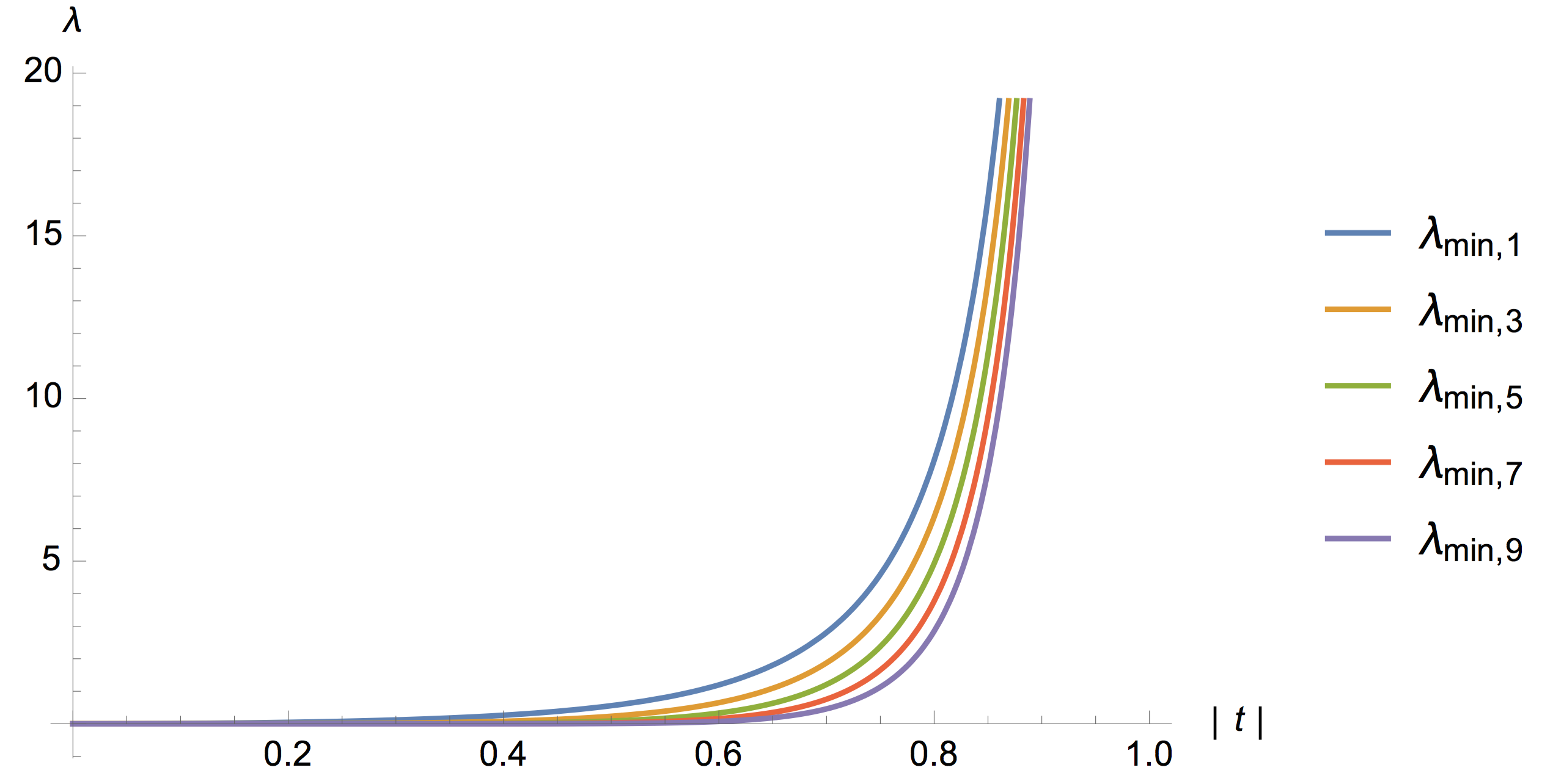
Figure 3.2. Smallest Non-Zero Eigenvalues for $k=1,3,5,7,9$.

4. Invariant Subspaces of $\mathcal{H}_{2k-1}(\mathbb{S}^{3})$ under $\square_{b}^{t}$

In this section we fix $k\geq 1$ and work on $\mathcal{H}_{2k-1}(\mathbb{S}^{3})$. As we have seen, $\square_{b}^{t}$ can be expanded in the following way:

$$\square_{b}^{t} =-(\mathcal{L}+\overline{t}\smash[b]{\overline{\mathcal{L}}})\frac{1+|t|^{2}}{(1-|t|^{2})^{2}}(\smash[b]{\overline{\mathcal{L}}}+t\mathcal{L})$$

$$=-h(\mathcal{L}\smash[b]{\overline{\mathcal{L}}}+|t|^{2}\smash[b]{\overline{\mathcal{L}}}\mathcal{L}+t\mathcal{L}^{2}+\overline{t}\smash[b]{\overline{\mathcal{L}}}^{2})$$ (1)

This is because of the linearity of $\mathcal{L}$ and $\smash[b]{\overline{\mathcal{L}}}$. Now, we need the following property.

Lemma 4.1.

If $\langle f_{i},f_{j}\rangle=0$ for $i\not=j$ and $f_{i},f_{j}\in\mathcal{H}_{0,2k-1}(\mathbb{S}^{3})$, then $\langle\smash[b]{\overline{\mathcal{L}}}^{\sigma}f_{i},\smash[b]{\overline{\mathcal{L}}}^{\sigma}f_{j}\rangle=0$ for $0\leq\sigma\leq 2k-1$.

Proof.

Choose $f_{i}$ and $f_{j}$, $i\not=j$ from an orthogonal basis for $\mathcal{H}_{0,2k-1}(\mathbb{S}^{3})$. We show that for $0\leq\sigma\leq 2k-1$, $\smash[b]{\overline{\mathcal{L}}}^{\sigma}f_{1}$ and $\smash[b]{\overline{\mathcal{L}}}^{\sigma}f_{j}$ are orthogonal. To do this we use induction on $\sigma$. Suppose $\langle\smash[b]{\overline{\mathcal{L}}}^{\sigma-1}f_{i},\smash[b]{\overline{\mathcal{L}}}^{\sigma-1}f_{j}\rangle=0$, and we show that $\langle\smash[b]{\overline{\mathcal{L}}}^{\sigma}f_{i},\smash[b]{\overline{\mathcal{L}}}^{\sigma}f_{j}\rangle=0$. Note that,

$$\langle\smash[b]{\overline{\mathcal{L}}}^{\sigma}f_{i},\smash[b]{\overline{\mathcal{L}}}^{\sigma}f_{j}\rangle =\langle\smash[b]{\overline{\mathcal{L}}}^{\sigma-1}f_{i},\mathcal{L}\smash[b]{\overline{\mathcal{L}}}^{\sigma}f_{j}\rangle$$

$$=\langle\smash[b]{\overline{\mathcal{L}}}^{\sigma-1}f_{i},(\mathcal{L}\smash[b]{\overline{\mathcal{L}}})\smash[b]{\overline{\mathcal{L}}}^{\sigma-1}f_{j}\rangle$$

$$=\langle\smash[b]{\overline{\mathcal{L}}}^{\sigma-1}f_{i},-\square_{b}\smash[b]{\overline{\mathcal{L}}}^{\sigma-1}f_{j}\rangle.$$

However since $\smash[b]{\overline{\mathcal{L}}}^{\sigma-1}f_{j}\in\mathcal{H}_{\sigma-1,2k-1-\sigma-1}(\mathbb{S}^{3})$, we know that $\square_{b}\smash[b]{\overline{\mathcal{L}}}^{\sigma-1}f_{j}=(\sigma)(2k-\sigma-2)\smash[b]{\overline{\mathcal{L}}}^{\sigma-1}f_{j}$. Therefore,

$$\langle\smash[b]{\overline{\mathcal{L}}}^{\sigma-1}f_{i},-\square_{b}\smash[b]{\overline{\mathcal{L}}}^{\sigma-1}f_{j}\rangle =\langle\smash[b]{\overline{\mathcal{L}}}^{\sigma-1}f_{i},-(\sigma)(2k-\sigma-2)\smash[b]{\overline{\mathcal{L}}}^{\sigma-1}f_{j}\rangle$$

$$=-(\sigma)(2k-\sigma-2)\langle\smash[b]{\overline{\mathcal{L}}}^{\sigma-1}f_{i},\smash[b]{\overline{\mathcal{L}}}^{\sigma-1}f_{j}\rangle$$

$$=0,$$

by our induction hypothesis as desired. ∎

With this, we first note that if $\{f_{0},\dotsc,f_{2k-1}\}$ is an orthogonal basis for $\mathcal{H}_{0,2k-1}(\mathbb{S}^{3})$, then $\{\smash[b]{\overline{\mathcal{L}}}^{\sigma}f_{0},\dotsc,\smash[b]{\overline{\mathcal{L}}}^{\sigma}f_{2k-1}\}$ is an orthogonal basis for $\mathcal{H}_{\sigma,2k-1-\sigma}(\mathbb{S}^{3})$. Now, we define the following subspaces of $\mathcal{H}_{2k-1}(\mathbb{S}^{3})$.

Definition 4.2.

Suppose $\{f_{0},\dotsc,f_{2k-1}\}$ is the orthogonal basis for $\mathcal{H}_{0,2k-1}(\mathbb{S}^{3})$. Then we define

$$V_{i}=\operatorname{span}\{f_{i},\smash[b]{\overline{\mathcal{L}}}^{2}f_{i},\ldots,\smash[b]{\overline{\mathcal{L}}}^{2j-2}f_{i},\dotsc,\smash[b]{\overline{\mathcal{L}}}^{2k-2}f_{i}\},$$

$$W_{i}=\operatorname{span}\{\smash[b]{\overline{\mathcal{L}}}f_{i},\smash[b]{\overline{\mathcal{L}}}^{3}f_{i},\ldots,\smash[b]{\overline{\mathcal{L}}}^{2j-1}f_{i},\dotsc,\smash[b]{\overline{\mathcal{L}}}^{2k-1}f_{i}\}.$$

Denote the basis elements of $V_{i}$ by $v_{i,1},\dotsc,v_{i,k}$ and for $W_{i}$ by $w_{i,1},\dotsc,w_{i,k}$. We first note that since each bidegree space $\mathcal{H}_{p,q}(\mathbb{S}^{3})\subseteq\mathcal{H}_{2k-1}(\mathbb{S}^{3})$ has $2k$ elements, we have $2k\;V_{i}$ spaces and $2k\;W_{i}$ spaces. We now note the following fact.

Theorem 4.3.

$\displaystyle\bigoplus_{i=0}^{2k-1}V_{i}\oplus W_{i}=\mathcal{H}_{2k-1}(\mathbb{S}^{3})$.

Proof.

We first note that by Theorem 2.7,

$$\mathcal{H}_{2k-1}(\mathbb{S}^{3}) =\bigoplus_{i=0}^{2k-1}\mathcal{H}_{i,2k-1-i}(\mathbb{S}^{3})$$

but by Lemma 4.1, we see that this is really just

$$=\bigoplus_{i=0}^{2k-1}\smash[b]{\overline{\mathcal{L}}}^{i}f_{0}\oplus\dotsb\oplus\smash[b]{\overline{\mathcal{L}}}^{i}f_{2k-1}.$$

Manipulating this, we have

$$=\bigoplus_{i=0}^{2k-1}f_{i}\oplus\smash[b]{\overline{\mathcal{L}}}f_{i}\dotsb\oplus\smash[b]{\overline{\mathcal{L}}}^{2k-1}f_{i}$$

$$=\bigoplus_{i=0}^{2k-1}f_{i}\oplus\smash[b]{\overline{\mathcal{L}}}^{2}f_{i}\oplus\dotsb\oplus\smash[b]{\overline{\mathcal{L}}}^{2k-2}f_{i}\oplus\smash[b]{\overline{\mathcal{L}}}f_{i}\oplus\smash[b]{\overline{\mathcal{L}}}^{3}f_{i}\oplus\dotsb\oplus\smash[b]{\overline{\mathcal{L}}}^{2k-1}f_{i}$$

$$=\bigoplus_{i=0}^{2k-1}V_{i}\oplus W_{i},$$

which is our goal. ∎

The advantage of constructing these spaces in the first place is due to the following fact.

Theorem 4.4.

$\square_{b}^{t}$ is invariant on $V_{i}$ and $W_{i}$.

Proof.

By equation (1), we have that

$$\square_{b}^{t}=-h(\mathcal{L}\smash[b]{\overline{\mathcal{L}}}+|t|^{2}\smash[b]{\overline{\mathcal{L}}}\mathcal{L}+t\mathcal{L}^{2}+\overline{t}\smash[b]{\overline{\mathcal{L}}}^{2})$$

Since the fraction in front is a constant, we can ignore it and only consider the expression in the parentheses. Let $f\in\mathcal{H}_{0,2k-1}(\mathbb{S}^{3})$, and define $v_{\sigma}=\smash[b]{\overline{\mathcal{L}}}^{\sigma}f$ to be a basis element of either $V_{i}$ or $W_{i}$, since they have the same form. We first note that $v_{\sigma}\in\mathcal{H}_{\sigma,2k-1-\sigma}(\mathbb{S}^{3})$. Then by our expansion we have that

$$\square_{b}^{t}v_{\sigma}=-h(\mathcal{L}\smash[b]{\overline{\mathcal{L}}}v_{\sigma}+|t|^{2}\smash[b]{\overline{\mathcal{L}}}\mathcal{L}v_{\sigma}+t\mathcal{L}^{2}v_{\sigma}+\overline{t}\smash[b]{\overline{\mathcal{L}}}^{2}v_{\sigma})$$

We already know $\mathcal{L}\smash[b]{\overline{\mathcal{L}}}v_{\sigma}$ and $\smash[b]{\overline{\mathcal{L}}}\mathcal{L}v_{\sigma}$ will simply be a multiple of $v_{\sigma}$, so we consider $\mathcal{L}^{2}v_{\sigma}$ and $\smash[b]{\overline{\mathcal{L}}}^{2}v_{\sigma}$.

$$\mathcal{L}^{2}v_{\sigma} =\mathcal{L}^{2}\smash[b]{\overline{\mathcal{L}}}^{\sigma}f$$

$$=\mathcal{L}\left[\mathcal{L}\smash[b]{\overline{\mathcal{L}}}\left[\smash[b]{\overline{\mathcal{L}}}^{\sigma-1}f\right]\right]$$

$$=-(\sigma)(2k-\sigma)\mathcal{L}\smash[b]{\overline{\mathcal{L}}}\left[\smash[b]{\overline{\mathcal{L}}}^{\sigma-2}f\right]$$

$$=(\sigma)(\sigma-1)(2k+1-\sigma)(2k-\sigma)\smash[b]{\overline{\mathcal{L}}}^{\sigma-2}f$$

$$=(\sigma)(\sigma-1)(2k+1-\sigma)(2k-\sigma)v_{\sigma-2}$$ (2a)

$$~{}\smash[b]{\overline{\mathcal{L}}}^{2}v_{\sigma} =\smash[b]{\overline{\mathcal{L}}}^{2}\left[\smash[b]{\overline{\mathcal{L}}}^{\sigma}f\right]$$

$$=\smash[b]{\overline{\mathcal{L}}}^{\sigma+2}f$$

$$=v_{\sigma+2}$$ (2b)

so we get multiples of $v_{\sigma-2}$ and $v_{\sigma+2}$. Relating this back to $V_{i}$ and $W_{i}$, we see that if $\sigma=2j-2$, then $\mathcal{L}^{2}v_{i,j}$ is a multiple of $v_{i,{j-1}}$, and $\smash[b]{\overline{\mathcal{L}}}^{2}v_{i,j}$ is a multiple of $v_{i,{j+1}}$. If $\sigma=2j-1$, we get a similar result for $w_{i,j}$. So we indeed have that $\square_{b}^{t}$ is invariant on $V_{i}$ and $W_{i}$, and we are done. ∎

In light of this fact, we can consider $\square_{b}^{t}$ not on the whole space $L^{2}(\mathbb{S}^{3})$ or $\mathcal{H}_{2k-1}(\mathbb{S}^{3})$, but rather on these $V_{i}$ and $W_{i}$ spaces. In fact, we actually have a representation of $\square_{b}^{t}$ on these spaces.

Theorem 4.5.

The matrix representation of $\square_{b}^{t}$, $m(\square_{b}^{t})$, on $V_{i}$ and $W_{i}$ is tridiagonal, where $m(\square_{b}^{t})$ on $V_{i}$ is

$$m(\square_{b}^{t})=h\begin{pmatrix}d_{1}&u_{1}&&&\phantom{\ddots}\\ -\overline{t}&d_{2}&u_{2}&&\phantom{\ddots}\\ &-\overline{t}&d_{3}&\ddots&\\ &&\ddots&\ddots&u_{k-1}\\ \phantom{\ddots}&&&-\overline{t}&d_{k}\end{pmatrix}$$

where $u_{j}=-t\cdot(2j)(2j-1)(2k-2j)(2k-1-2j)$ and $d_{j}=(2j-1)(2k+1-2j)+|t|^{2}\cdot(2j-2)(2k+2-2j)$. For $W_{i}$, we get something similar:

$$m(\square_{b}^{t})=h\begin{pmatrix}d_{1}&u_{1}&&&\phantom{\ddots}\\ -\overline{t}&d_{2}&u_{2}&&\phantom{\ddots}\\ &-\overline{t}&d_{3}&\ddots&\\ &&\ddots&\ddots&u_{k-1}\\ \phantom{\ddots}&&&-\overline{t}&d_{k}\end{pmatrix}$$

where $u_{j}=-t\cdot(2j+1)(2j)(2k-2j)(2k-1-2j)$ and $d_{j}=(2j)(2k-2j)+|t|^{2}\cdot(2j-1)(2k+1-2j)$.

We note that the above definitions don’t depend on $i$; in other words, each of these matrices are the same on $V_{i}$ and $W_{i}$, regardless of the choice of $i$.

Proof.

Using equations (2a) and (2b), along with Theorem 2.9, we can entirely describe the action of each piece of $\square_{b}^{t}$ on a basis element $v_{i,j}$ or $w_{i,j}$:

$$-\mathcal{L}\smash[b]{\overline{\mathcal{L}}}v_{i,j} =(2j-1)(2k+1-2j)v_{i,j} -\mathcal{L}\smash[b]{\overline{\mathcal{L}}}w_{i,j} =(2j)(2k-2j)w_{i,j}$$

$$-\smash[b]{\overline{\mathcal{L}}}\mathcal{L}v_{i,j} =(2j-2)(2k+2-2j)v_{i,j} -\smash[b]{\overline{\mathcal{L}}}\mathcal{L}w_{i,j} =(2j-1)(2k+1-2j)w_{i,j}$$

$$\begin{split}-\mathcal{L}^{2}v_{i,j}&=-(2j-2)(2j-3)\\ &\hskip 21.00009pt(2k+3-2j)(2k+2-2j)v_{i,{j-1}}\end{split} \begin{split}-\mathcal{L}^{2}w_{i,j}&=-(2j-1)(2j-2)\\ &\hskip 21.00009pt(2k+2-2j)(2k+1-2j)w_{i,{j-1}}\end{split}$$

$$-\smash[b]{\overline{\mathcal{L}}}^{2}v_{i,j} =-v_{i,{j+1}} -\smash[b]{\overline{\mathcal{L}}}^{2}w_{i,j} =-w_{i,{j+1}}.$$

By looking at it this way, we notice the tridiagonal structure. So with these observations, we can state that

$$\begin{split}\square_{b}^{t}v_{i,j}=h\big{(}&-t\cdot(2j-2)(2j-3)(2k+3-2j)(2k+2-2j)v_{i,{j-1}}\\ &+\left((2j-1)(2k+1-2j)+|t|^{2}\cdot(2j-2)(2k+2-2j)\right)\!v_{i,j}\\ &-\overline{t}\cdot v_{i,{j+1}}\,\big{)}\end{split}$$

$$\begin{split}\square_{b}^{t}w_{i,j}=h\big{(}&-t\cdot(2j-1)(2j-2)(2k+2-2j)(2k+1-2j)w_{i,{j-1}}\\ &+\left((2j)(2k-2j)+|t|^{2}\cdot(2j-1)(2k-1-2j)\right)\!w_{i,j}\\ &-\overline{t}\cdot w_{i,{j+1}}\,\big{)}.\end{split}$$

Now that we have this formula, we can find $m(\square_{b}^{t})$ on $V_{i}$ and $W_{i}$ by computing their effect on the basis vectors $v_{i,j}$ and $w_{i,j}$: when we do this for $V_{i}$, we get

$$d_{j} =(2j-1)(2k+1-2j)+|t|^{2}\cdot(2j-2)(2k+2-2j)$$

$$u_{j-1} =-t\cdot(2j-2)(2j-3)(2k+3-2j)(2k+2-2j)$$

$$\implies u_{j}=-t\cdot(2j)(2j-1)(2k-2j)(2k-1-2j)$$

and for $W_{i}$, we get

$$d_{j} =(2j)(2k-2j)+|t|^{2}\cdot(2j-1)(2k-1-2j)$$

$$u_{j-1} =-t\cdot(2j-1)(2j-2)(2k+2-2j)(2k+1-2j)$$

$$\implies u_{j}=-t\cdot(2j+1)(2j)(2k-2j)(2k-1-2j).$$

Finally, by factoring out $h$ and simply substituting each portion in we obtain the matrix representations above. ∎

An immediate consequence of this is that each $V_{i}$ subspace contributes the same set of eigenvalues to the spectrum of $\square_{b}^{t}$, and similarly for each $W_{i}$. Furthermore, we note that the matrices are rank $k$. Since the choice of $i$ does not change $m(\square_{b}^{t})$ on these spaces, we will fix an arbitrary $i$ and call the spaces $V$ and $W$ instead.

5. Bottom of the Spectrum of $\square_{b}^{t}$

Now that we have a matrix representation for $\square_{b}^{t}$ on these $V$ and $W$ spaces inside $\mathcal{H}_{2k-1}(\mathbb{S}^{3})$, we can begin to analyze their eigenvalues as $k$ varies. First, we go over some facts about tridiagonal matrices.

Theorem 5.1.

Suppose $A$ is a tridiagonal matrix,

$$A=\begin{pmatrix}d_{1}&u_{1}&&&\phantom{\ddots}\\ l_{1}&d_{2}&u_{2}&&\phantom{\ddots}\\ &l_{2}&d_{3}&\ddots&\\ &&\ddots&\ddots&u_{k-1}\\ \phantom{\ddots}&&&l_{k-1}&d_{k}\end{pmatrix}$$

and the products $u_{i}l_{i}>0$ for $1\leq i\leq k$, then $A$ is similar to a symmetric tridiagonal matrix.

Proof.

One can verify that if

$$S=\begin{pmatrix}1&&&&\phantom{\ddots}\\ &\sqrt{\frac{u_{1}}{l_{1}}}&&&\phantom{\ddots}\\ &&\sqrt{\frac{u_{1}u_{2}}{l_{1}l_{2}}}&&\phantom{\ddots}\\ &&&\ddots&\\ \phantom{\ddots}&&&&\sqrt{\frac{u_{1}\dotsb u_{k-1}}{l_{1}\dotsb l_{k-1}}}\end{pmatrix}$$

then $A=SBS^{{-1}}$, where

$$B=\begin{pmatrix}d_{1}&\sqrt{u_{1}l_{1}}&&&\phantom{\ddots}\\ \sqrt{u_{1}l_{1}}&d_{2}&\sqrt{u_{2}l_{2}}&&\phantom{\ddots}\\ &\sqrt{u_{2}l_{2}}&d_{3}&\ddots&\\ &&\ddots&\ddots&\sqrt{u_{k-1}l_{k-1}}\\ \phantom{\ddots}&&&\sqrt{u_{k-1}l_{k-1}}&d_{k}\end{pmatrix}$$

Therefore, $A$ is similar to a symmetric tridiagonal matrix. ∎

Another special property of tridiagonal matrices is the continuant.

Definition 5.2.

Let $A$ be a tridiagonal matrix, like the above. Then we define the continuant of $A$ to be a recursive sequence: $f_{1}=d_{1}$, and $f_{i}=d_{i-1}f_{i-1}-u_{i-2}l_{i-2}f_{i-2}$, where $f_{0}=1$.

The reason we define this is because $\det(A)=f_{k}$. In addition, if we denote $A_{i}$ to mean the square submatrix of $A$ formed by the first $i$ rows and columns, then $\det(A_{i})=f_{i}$.
With this background, we will now start analyzing $\square_{b}^{t}$ on $W$.

To get bounds on the eigenvalues, we will invoke the Cauchy interlacing theorem, see [Hwa04].

Theorem 5.3.

Suppose $A$ is an $n\times n$ Hermitian matrix of rank $n$, and $B$ is an $n-1\times n-1$ matrix minor of $A$. If the eigenvalues of $A$ are $\lambda_{1}\leq\dotsb\leq\lambda_{n}$ and the eigenvalues of $B$ are $\nu_{1}\leq\dotsb\leq\nu_{n-1}$, then the eigenvalues of $A$ and $B$ interlace:

$$0<\lambda_{1}\leq\nu_{1}\leq\lambda_{2}\leq\nu_{2}\leq\dotsb\leq\lambda_{n-1}\leq\nu_{n-1}\leq\lambda_{n}$$

Now, we can get an intermediate bound on the smallest eigenvalue.

Theorem 5.4.

Suppose $A$ is a Hermitian matrix of rank $n$, and $\lambda_{1}\leq\dotsb\leq\lambda_{n}$ are its eigenvalues. Then

$$\lambda_{1}\leq\frac{\det(A)}{\det(A_{k-1})}$$

where $A_{k-1}$ is $A$ without the last row and column.

Proof.

Since $A_{k-1}$ is a $k-1\times k-1$ matrix minor of $A$, we can apply the Cauchy interlacing theorem. If the eigenvalues of $A_{k-1}$ are $\nu_{1}\leq\dotsb\leq\nu_{k-1}$, then

$$\lambda_{1}\leq\nu_{1}\leq\lambda_{2}\leq\nu_{2}\leq\dotsb\leq\lambda_{n-1}\leq\nu_{n-1}\leq\lambda_{n}$$

Now, we claim that

$$\lambda_{1}\det(A_{k-1})\leq\det(A)$$

To see why this is true, first observe that the determinant of a matrix is simply the product of all its eigenvalues. In particular,

$$\lambda_{1}\det(A_{k-1})=\lambda_{1}\nu_{1}\dotsb\nu_{k-1}$$

But we can simply apply the Cauchy interlacing theorem: since $\nu_{1}\leq\lambda_{2}$, $\nu_{2}\leq\lambda_{3}$, and so on, we get

$$\lambda_{1}\nu_{1}\dotsb\nu_{k-1} \leq\lambda_{1}\lambda_{2}\dotsb\lambda_{k}$$

$$=\det(A)$$

so the claim is proven. Now, dividing both sides by $\det A_{k-1}$,

$$\lambda_{1}\leq\frac{\det(A)}{\det(A_{k-1})}$$

as desired. ∎

Since $m(\square_{b}^{t})$ on $W$ satisfies the conditions of Theorem 5.1, we find it is similar to this Hermitian tridiagonal matrix:

$$A=\begin{pmatrix}a_{1}+b_{1}|t|^{2}&c_{1}|t|&&&\phantom{\ddots}\\ c_{1}|t|&a_{2}+b_{2}|t|^{2}&c_{2}|t|&&\phantom{\ddots}\\ &c_{2}|t|&a_{3}+b_{3}|t|^{2}&\ddots&\\ &&\ddots&\ddots&c_{k-1}|t|\\ \phantom{\ddots}&&&c_{k-1}|t|&a_{k}+b_{k}|t|^{2}\end{pmatrix}$$

where $a_{i}=(2i)(2k-2i)$, $b_{i}=(2i-1)(2k+1-2i)$, and $c_{i}=\sqrt{(2i+1)(2i)(2k-2i)(2k-1-2i)}$. Note that we are ignoring the constant $h$ for now, which we will add back later. If we can find $\det(A_{i})$, then by Theorem 5.4 we can get a closed form for the bound on the smallest eigenvalue. With the following lemma, this is possible:

Lemma 5.5.

$a_{i}b_{i+1}=c_{i}^{2}$

Proof.

We can simply work through the formulas to figure this out: $a_{i}=(2i)(2k-2i)$, $b_{i+1}=(2i+1)(2k-1-2i)$, and $c_{i}^{2}=(2i+1)(2i)(2k-2i)(2k-1-2i)$. The products clearly match up. ∎

Theorem 5.6.

The determinant of $A_{i}$ is

$$\begin{split}\det(A_{i})&=a_{1}a_{2}\dotsb a_{i-1}a_{i}\\ &+b_{1}a_{2}\dotsb a_{i-1}a_{i}|t|^{2}\\ &+\dotsb\\ &+b_{1}b_{2}\dotsb b_{i-1}a_{i}|t|^{2i-2}\\ &+b_{1}b_{2}\dotsb b_{i-1}b_{i}|t|^{2i}\end{split}$$

In each row, we replace a particular $a_{j}$ with $b_{j}$, and multiply by $|t|^{2}$. Note that if $i=k$, then $a_{k}=0$ and all terms but the last term are 0.

Proof.

We will prove this using strong induction on $i$. The base case is $i=1$, where $\det(A_{1})=a_{1}+b_{1}|t|^{2}$, which does indeed match up with our formula. Now, assume the formula works for $A_{i-1}$ and $A_{i}$. We need to show that the formula works for $A_{i+1}$. Using the formula for the continuant, we get

$$\det(A_{i+1}) =(a_{i+1}+b_{i+1}|t|^{2})\det(A_{i})-c_{i}^{2}|t|^{2}\det(A_{i-1})$$

Now, use Lemma 5.5:

$$=(a_{i+1}+b_{i+1}|t|^{2})\det(A_{i})-a_{i}b_{i+1}|t|^{2}\det(A_{i-1})$$

Now, we use our induction hypothesis:

$$= \;(a_{i+1}+b_{i+1}|t|^{2})(a_{1}a_{2}\dotsb a_{i}+b_{1}a_{2}\dotsb a_{i}|t|^{2}+\dotsb+b_{1}b_{2}\dotsb b_{i}|t|^{2i})$$

$$-a_{i}b_{i+1}|t|^{2}(a_{1}a_{2}\dotsb a_{i-1}+b_{1}a_{2}\dotsb a_{i-1}|t|^{2}+\dotsb+b_{1}b_{2}\dotsb b_{i-1}|t|^{2i-2})$$

$$= \;a_{1}a_{2}\dotsb a_{i+1}+b_{1}a_{2}\dotsb a_{i+1}|t|^{2}+\dotsb+b_{1}b_{2}\dotsb b_{i}a_{i+1}|t|^{2i}$$

$$+a_{1}a_{2}\dotsb a_{i}b_{i+1}|t|^{2}+b_{1}a_{2}\dotsb a_{i}b_{i+1}|t|^{4}+\dotsb+b_{1}b_{2}\dotsb b_{i-1}a_{i}b_{i+1}|t|^{2i+2}+b_{1}b_{2}\dotsb b_{i+1}|t|^{2i+2}$$

$$-a_{1}a_{2}\dotsb a_{i}b_{i+1}|t|^{2}-b_{1}a_{2}\dotsb a_{i}b_{i+1}|t|^{4}-\dotsb-b_{1}b_{2}\dotsb b_{i-1}a_{i}b_{i+1}|t|^{2i+2}$$

$$= \;a_{1}a_{2}\dotsb a_{i+1}+b_{1}a_{2}\dotsb a_{i+1}|t|^{2}+\dotsb+b_{1}b_{2}\dotsb b_{i}a_{i+1}|t|^{2i}+b_{1}b_{2}\dotsb b_{i+1}|t|^{2i+2}$$

which is the formula for $A_{i+1}$, and we are done. ∎

With this knowledge, we are finally able to prove our theorem.

Theorem 5.7.

$0\in\operatorname{essspec}(\square_{b}^{t})$

Proof.

By Theorem 5.6, we have that on $W$ in $\mathcal{H}_{2k-1}(\mathbb{S}^{3})$, $m(\square_{b}^{t})$ is similar to

$$A=h\begin{pmatrix}a_{1}+b_{1}|t|^{2}&c_{1}|t|&&&\phantom{\ddots}\\ c_{1}|t|&a_{2}+b_{2}|t|^{2}&c_{2}|t|&&\phantom{\ddots}\\ &c_{2}|t|&a_{3}+b_{3}|t|^{2}&\ddots&\\ &&\ddots&\ddots&c_{k-1}|t|\\ \phantom{\ddots}&&&c_{k-1}|t|&a_{k}+b_{k}|t|^{2}\end{pmatrix}$$

where $a_{j}=(2j)(2k-2j)$, $b_{j}=(2j-1)(2k+1-2j)$, and $c_{j}=\sqrt{(2j+1)(2j)(2k-2j)(2k-1-2j)}$. Now, by Theorem 5.4 above, we know that

$$\lambda_{\min}\leq\frac{\det(A)}{\det(A_{k-1})}.$$

Recall that $A_{k-1}$ denotes the submatrix formed by deleting the last row and column of the $k\times k$ matrix $A$. To show that $0\in\operatorname{essspec}(\square_{b}^{t})$, we want to show that $\det(A)/\det(A_{k-1})\to 0$ as $k\to\infty$. For this purpose we find an upper bound for $\det(A)/\det(A_{k-1})$ and show that this converges to $0$. Notice that Theorem 5.6 implies that,

$$\frac{\det(A)}{\det(A_{k-1})} =h\frac{b_{1}b_{2}\dots b_{k-1}b_{k}|t|^{2k}}{a_{1}a_{2}\dots a_{k-1}+b_{1}a_{2}\dots a_{k-1}|t|^{2}+b_{1}b_{2}\dots a_{k-1}|t|^{4}+\dots b_{1}b_{2}\dots b_{k-1}|t|^{2k-2}}$$

$$\leq h\frac{b_{1}b_{2}\dots b_{k-1}b_{k}|t|^{2k}}{a_{1}a_{2}\dots a_{k-1}}.$$ (3)

since, $a_{j},b_{j},|t|>0$. Now using the formulas for $a_{j}$ and $b_{j}$, notice that $($5$)$ can be written as

$$h(2k-1)|t|^{2k}\prod_{j=1}^{k-1}\frac{(2j+1)(2k-2j-1)}{(2j)(2k-2j)}.$$

However, we know that for all $k$ and $1\leq j\leq k-1,$

$$\frac{(2k-2j-1)}{(2k-2j)}<1,$$

and so,

$$h(2k-1)|t|^{2k}\prod_{j=1}^{k-1}\frac{(2j+1)(2k-2j-1)}{(2j)(2k-2j)}\leq h(2k-1)|t|^{2k}\prod_{j=1}^{k-1}\frac{(2j+1)}{(2j)}=h(2k-1)|t|^{2k}\prod_{j=1}^{k-1}1+\frac{1}{2j}.$$

Furthermore, we have

$$h(2k-1)|t|^{2k}\prod_{j=1}^{k-1}1+\frac{1}{2j}\leq h(2k-1)|t|^{2k}\exp\left(\sum_{j=1}^{k-1}\frac{1}{2j}\right).$$

Note that

$$\sum_{j=1}^{k-1}\frac{1}{2j}\leq\frac{1}{2}\ln k$$

so our expression becomes

$$\frac{\det(A)}{\det(A_{k-1})}\leq h(2k-1)|t|^{2k}\exp\left(\frac{1}{2}\ln k\right)=h(2k-1)\sqrt{k}\,|t|^{2k}$$

and our problem reduces to showing that $\lim\limits_{k\to\infty}h(2k-1)\sqrt{k}|t|^{2k}=0$. We note that $h$ is a constant and $|t|<1$; therefore, by L’Hospital’s rule the last expression indeed goes to $0$.

Finally, we have,

$$0\leq\lim_{k\to\infty}\lambda_{\min}\leq\lim_{k\to\infty}\frac{\det(A)}{\det(A_{k-1})}\leq\lim_{k\to\infty}h(2k-1)\sqrt{k}\,|t|^{2k}=0,$$

and so $\lambda_{\min}\to 0$. Hence $0\in\operatorname{essspec}(\square_{b}^{t}).$ ∎

We note that by the discussion in the introduction, this means that the CR-manifold $(\mathcal{L}_{t},\mathbb{S}^{3})$ is not embeddable into any $\mathbb{C}^{N}$.

References

• [ABR01] Sheldon Axler, Paul Bourdon, and Wade Ramey. Harmonic function theory, volume 137 of Graduate Texts in Mathematics. Springer-Verlag, New York, second edition, 2001.
• [BdM75] L. Boutet de Monvel. Intégration des équations de Cauchy-Riemann induites formelles. pages Exp. No. 9, 14, 1975.
• [BE90] Daniel M. Burns and Charles L. Epstein. Embeddability for three-dimensional CR-manifolds. J. Amer. Math. Soc., 3(4):809–841, 1990.
• [Bog91] A. Boggess. CR Manifolds and the Tangential Cauchy Riemann Complex. Studies in Advanced Mathematics. Taylor & Francis, 1991.
• [Bur79] Daniel M. Burns, Jr. Global behavior of some tangential Cauchy-Riemann equations. In Partial differential equations and geometry (Proc. Conf., Park City, Utah, 1977), volume 48 of Lecture Notes in Pure and Appl. Math., pages 51–56. Dekker, New York, 1979.
• [CS01] S.C. Chen and M.C. Shaw. Partial Differential Equations in Several Complex Variables. AMS/IP studies in advanced mathematics. American Mathematical Society, 2001.
• [Fu05] Siqi Fu. Hearing pseudoconvexity with the Kohn Laplacian. Math. Ann., 331(2):475–485, 2005.
• [Fu08] Siqi Fu. Hearing the type of a domain in $\mathbb{C}^{2}$ with the $\overline{\partial}$-Neumann Laplacian. Adv. Math., 219(2):568–603, 2008.
• [Hwa04] Suk-Geun Hwang. Cauchy’s interlace theorem for eigenvalues of Hermitian matrices. Amer. Math. Monthly, 111(2):157–159, 2004.
• [Koh85] J. J. Kohn. Estimates for $\bar{\partial}_{b}$ on pseudoconvex CR manifolds. In Pseudodifferential operators and applications (Notre Dame, Ind., 1984), volume 43 of Proc. Sympos. Pure Math., pages 207–217. Amer. Math. Soc., Providence, RI, 1985.
• [Ros65] H. Rossi. Attaching analytic spaces to an analytic space along a pseudoconcave boundary. In Proc. Conf. Complex Analysis (Minneapolis, 1964), pages 242–256. Springer, Berlin, 1965.