Far-from-Equilibrium Time Evolution between two Gamma Distributions

Abstract

Many systems in nature and laboratories are far from equilibrium and exhibit significant fluctuations, invalidating the key assumptions of small fluctuations and short memory time in or near equilibrium. A full knowledge of Probability Distribution Functions (PDFs), especially time-dependent PDFs, becomes essential in understanding far-from-equilibrium processes. We consider a stochastic logistic model with multiplicative noise, which has gamma distributions as stationary PDFs. We numerically solve the transient relaxation problem, and show that as the strength of the stochastic noise increases the time-dependent PDFs increasingly deviate from gamma distributions. For sufficiently strong noise a transition occurs whereby the PDF never reaches a stationary state, but instead forms a peak that becomes ever more narrowly concentrated at the origin. The addition of an arbitrarily small amount of additive noise regularizes these solutions, and re-establishes the existence of stationary solutions. In addition to diagnostic quantities such as mean value, standard deviation, skewness and kurtosis, the transitions between different solutions are analyzed in terms of entropy and information length, the total number of statistically distinguishable states that a system passes through in time.

I Introduction

In classical statistical mechanics, the Gaussian (or normal) distribution and mean-field type theories based on such distributions have been widely used to describe equilibrium or near equilibrium phenomena. The ubiquity of the Gaussian distribution stems from the central limit theorem that random variables governed by different distributions tend to follow the Gaussian distribution in the limit of large sample size Fokker ; Klebaner ; Gardiner . In such a limit, fluctuations are small and have a short correlation time, and mean values and variance completely describe all different moments, greatly facilitating analysis.

Many systems in nature and laboratories are however far from equilibrium, exhibiting significant fluctuations. Examples are found not only in turbulence in astrophysical and laboratory plasmas, but also in forest fires, the stock market, and biological ecosystems nature ; KIM02 ; KIM03 ; KIM06 ; KIM08 ; KIM13 ; SrinYoun2011 ; SayaShowDowl2008 ; tsuchiya15 ; tang88 ; Jensen98 ; Pruesser12 ; Longo11 ; FLYNN2014 ; FLYNN2015 ; Ovidiu ; Shahrezaei ; Thomas ; Biswas ; Elgart . Specifically, anomalous (much larger than average values) transport associated with large fluctuations in fusion plasmas can degrade the confinement, potentially even terminating fusion operation KIM03 . Tornadoes are rare, large amplitude events, but can cause very substantial damage when they do occur. In biology, the pioneering work of Delbrück on bacteriophages showed that viruses replicate in strongly fluctuating bursts delbruck1945burst . The fluctuations of the burst amplitudes were explained mathematically by stochastic autocatalytic reaction models first introduced in delbruck1940statistical . Delbrück’s autocatalytic models predict discrete negative-binomial distributions, that can be well approximated by gamma distributions when the average number of particles is large. Furthermore, gene expression and protein productions, which used to be thought of as smooth processes, have also been observed to occur in bursts leading to negative binomial and gamma distributed protein copy numbers (e.g. Ovidiu ; Shahrezaei ; Thomas ; Biswas ; Elgart ). Such rare events of large amplitude (called intermittency) can dominate the entire transport even if they occur infrequently KIM08 ; KIM09 . They thus invalidate the assumption of small fluctuations with short correlation time, making mean value and variances meaningless. Therefore, to understand the dynamics of a system far from equilibrium, it is crucial to have a full knowledge of Probability Distribution Functions (PDFs), including time-dependent PDFs KH16 .

The consequences of strong fluctuations in far-from-equilibrium systems are multiple. In physics, far-from-equilibrium fluctuations produce dissipative patterns, shift or wipe out phase transitions, etc. In economics, finance and actuarial science, strong fluctuations are important issues of risk evaluation. In biology, strong fluctuations generate phenotypic heterogeneity that helps multicellular organisms or microbial populations to adapt to changes of the environment by so-called “bet-hedging” strategies. In such a strategy, only a part of the cell population adapts upon emergence of new environmental conditions. The remaining part retains the memory of the old conditions and is thus already adapted if environmental conditions revert to previous ones de2011bet . Exceptional behavior can also rescue cell subpopulations from drug-induced lethal conditions, thus generating drug resistance balaban2004bacterial . In particular, because of the skewness and exponential tail of the gamma distribution, gamma distributed populations contain a significant proportion of individuals with exceptionally high phenotype. Bet-hedging being a dynamic phenomenon, it is important, for biological studies, to be able to predict not only steady-state but also time-dependent distributions.

Obtaining a good quality of PDFs is often very challenging, as it requires a sufficiently large number of simulations or observations. Therefore, a PDF is usually constructed by averaging data from a long time series, and is thus stationary (independent of time). Unfortunately, such stationary PDFs miss crucial information about the dynamics/evolution of non-equilibrium processes (e.g. tumour evolution). Theoretical prediction of time-dependent PDFs has proven to be no less challenging due to the limitation in our understanding of nonlinear stochastic dynamical systems as well as the complexity in the required analysis.

Spectral analysis, for example, using theoretical tools similar to those used in quantum mechanics (e.g. raising and lower operators) is useful (e.g. Fokker ), but the summation of all eigenfunctions is necessary for time-dependent PDFs far from equilibrium. Various different methodologies have also been developed to obtain approximate PDFs, such as the variational principle, the rate equation method, or moment method prigogine ; suzuki80 ; suzuki81 ; langer75 ; saito76 ; hasegawa77 . In particular, the rate equation method suzuki80 ; suzuki81 assumes that the form of a time-dependent PDF during the relaxation is similar to that of the stationary PDF, and thus approximates a time-dependent PDF during transient relaxation by a PDF having the same functional form as a stationary PDF, but with time-varying parameters.

In this work we show that this assumption is not always appropriate. We consider a stochastic logistic model with multiplicative noise. We show that for fixed parameter values the stationary PDFs are always gamma distributions (e.g. dennis ; liao ), one of the most popular distributions used in fitting experimental data. However, we find numerically that the time-dependent PDFs in transitioning from one set of parameter values to another are significantly different from gamma distributions, especially for strong stochastic noise. For sufficiently strong multiplicative noise it is necessary to introduce additive noise as well to obtain stationary distributions at all. We note that in inferential statistics, gamma distributions facilitate Bayesian model learning from data, as a gamma distribution is a conjugate prior to many likelihood functions. It is therefore interesting to test whether models with stationary gamma distributions also have time-dependent gamma distributions.

II Stochastic Logistic Model

We consider the logistic growth with a multiplicative noise given by the following Langevin equation:

$$\frac{dx}{dt}=(\gamma+\xi)x-\epsilon x^{2},$$ (1)

where $x$ is a random variable, and $\xi$ is a stochastic forcing, which for simplicity can be taken as a short-correlated random forcing as follows:

$$\langle\xi(t)\xi(t^{\prime})\rangle={2D}\delta(t-t^{\prime}).$$ (2)

In Eq. (2), the angular brackets represent the average over $\xi$, $\langle{\xi}\rangle=0$, and $D$ is the strength of the forcing. $\gamma$ is the control parameter in the positive feedback, representing the growth rate of $x$, while $\epsilon$ represents the efficiency in self-regulation by a negative feedback. $\gamma x-\epsilon x^{2}$ can be considered as the gradient of the potential $V$ as $\gamma x-\epsilon x^{2}=-\frac{\partial V}{\partial x},$ where $V=-\frac{\gamma}{2}x^{2}+\frac{\epsilon}{3}x^{3}$. Thus, $V$ has its minimum value at $x=\frac{\gamma}{\epsilon}$. When $\xi=0$, $x=\frac{\gamma}{\epsilon}$ (the carrying capacity) is a stable equilibrium point since $\partial_{{xx}}V\Bigr{|}_{x={\gamma}/{\epsilon}}=\gamma>0$; $x=0$ is an unstable equilibrium point since $\partial_{xx}V\Bigr{|}_{{x=0}}=-\gamma<0$. The multiplicative noise in Eq. (1) shows that the linear growth rate contains the stochastic part $\xi$. This model is entirely phenomenological and $x$ can be interpreted as the size of a critical physical phenomenon (vortex, tornado, etc.), stock market, number of biological cells, viruses, proteins. It is reminiscent of Delbrück’s autocatalytic processes delbruck1940statistical , but is different from these in many ways, the most important being the lack of discreteness and the possibility of reaching a steady state due to the finite capacity of logistic growth. We will show in the following that in spite of these differences, our model is capable of producing large fluctuations.

By using the Stratonovich calculus Klebaner ; Gardiner ; WongZakai , we can obtain the following Fokker-Planck equation for the PDF $p(x,t)$ (see Appendix A for details):

$$\frac{\partial}{\partial t}\,p(x,t)=-\frac{\partial}{\partial x}\Bigl{[}(\gamma x-\epsilon x^{2})p(x,t)\Bigr{]}+D\,\frac{\partial}{\partial x}\left[x\,\frac{\partial}{\partial x}\Bigl{[}x\,p(x,t)\Bigr{]}\right]$$ (3)

corresponding to the Langevin equation (1). By setting $\partial_{t}p=0$, we can analytically solve for the stationary PDFs as

$$p(x)=\frac{b^{a}}{\Gamma(a)}x^{{a-1}}e^{-bx},$$ (4)

which is the well-known gamma distribution. The two parameters $a$ and $b$ are given by $a={\gamma}/{D}$ and $b={\epsilon}/{D}$. The mean value and variance of the gamma distribution are found to be:

$$\langle x\rangle=\frac{a}{b}=\frac{\gamma}{\epsilon},\qquad\qquad{\rm Var}(x)=\sigma^{2}=\langle(x-\langle x\rangle)^{2}\rangle=\frac{a}{b^{2}}=\frac{\gamma D}{\epsilon^{2}},$$ (5)

where $\sigma=\sqrt{{\rm Var}(x)}$ is the standard deviation. We recognise $\langle x\rangle$ as the carrying capacity for a deterministic system with $\xi=0$. It is useful to note that $\langle x\rangle$ is given by the linear growth rate scaled by $\epsilon$, while ${{\rm Var}(x)}$ is given by the product of the linear growth rate and the diffusion coefficient, each scaled by $\epsilon$. That is, the effect of stochasticity should be measured relative to the linear growth rate.

Therefore, the case of small fluctuations is modelled by values of $D$ small compared with $\gamma$ and $\epsilon$. In such a limit, $a$ and $b$ are large, making $\sqrt{{\rm Var}(x)}\ll\langle x\rangle$ in Eq. (5). That is, the width of the PDF is much smaller than its mean value. In this limit, Eq. (4) reduces to a Gaussian distribution. To show this, we express Eq. (4) in the following form:

$$p\equiv\frac{b^{a}}{\Gamma(a)}e^{-f(x)},$$ (6)

where $f(x)=bx-(a-1)\ln{x}$. For large $b$, we expand $f(x)$ around the stationary point $x=x_{p}$ where $\partial_{x}f(x)=0=b-(a-1)/x$ up to the second order in $x-x_{p}$ to find:

$$x_{p}=\frac{a-1}{b}\sim\frac{a}{b},\qquad\qquad f(x=x_{p})\sim a\left(1-\ln{\frac{a}{b}}\right),$$ (7)

$$f(x)\sim f(x_{p})+\frac{1}{2}(x-x_{p})^{2}\partial_{xx}f(x)\Big{|}_{x=x_{p}}=a\left(1-\ln{\frac{a}{b}}\right)+\frac{b^{2}}{2a}\left(x-\frac{a}{b}\right)^{2}.$$ (8)

Here $a\gg 1$ was used. Using Eq. (8) in Eq. (6) then gives us

$$p\propto\exp{\left[-\frac{b^{2}}{2a}\left(x-\frac{a}{b}\right)^{2}\right]}\propto\exp{\Bigl{[}-\beta(x-\langle x\rangle)^{2}\Bigr{]}},$$ (9)

which is a Gaussian PDF with mean value $\langle x\rangle$. Here $\beta={1}/{{\rm Var}(x)}$ is the inverse temperature and the variance ${\rm Var}(x)$ is given by Eq. (5). Therefore, for a sufficiently small $D$, the gamma distribution is approximated as a Gaussian PDF, which is consistent with the central limit theorem as small $D$ corresponds to small fluctuations and large system size. See also bagui for a different derivation.

As $D$ increases, the Gaussian approximation becomes increasingly less valid. Indeed, even the gamma distribution becomes invalid asymptotically, when $t\to\infty$, if $D>\gamma$; according to Eq. (4) having $a<1$ yields $\displaystyle\lim_{x\to 0}p=\lim_{x\to 0}\frac{\partial p}{\partial x}=\infty$. However, from the full time-dependent Fokker-Planck equation (3) one finds that if the initial condition satisfies $p=0$ at $x=0$, then $p(x=0)$ will remain 0 for all later times. As we will see, the resolution to this seeming paradox is that no stationary distribution is ever reached for $D>\gamma$, but instead the peak approaches ever closer to $x=0$, without ever reaching it.

If we are interested in obtaining stationary solutions even when $D>\gamma$, one way to achieve that is to return to the original Langevin equation (1), but now include a further additive stochastic noise $\eta$:

$$\frac{dx}{dt}=(\gamma+\xi)x-\epsilon x^{2}+\eta,$$ (10)

where $\xi$ and $\eta$ are uncorrelated, and $\eta$ satisfies $\langle\eta(t)\eta(t^{\prime})\rangle=2Q\delta(t-t^{\prime})$. The new version of the Fokker-Planck equation (3) then becomes:

$$\frac{\partial}{\partial t}\,p=-\frac{\partial}{\partial x}\Bigl{[}(\gamma x-\epsilon x^{2})p\Bigr{]}+D\,\frac{\partial}{\partial x}\left[x\,\frac{\partial}{\partial x}\Bigl{[}x\,p\Bigr{]}\right]+Q\frac{\partial^{2}}{\partial x^{2}}\,p,$$ (11)

which has stationary solutions given by

$$\ln p(x)=\int\frac{(\gamma-D)x-\epsilon x^{2}}{Dx^{2}+Q}\,dx.$$ (12)

This integral can be evaluated analytically, but the final form is not particularly illuminating. The only point to note is that for non-zero $Q$ the denominator is never 0 even for $x\to 0$, which avoids any possible singularities at the origin. For $\gamma>D$ and $Q\ll D$ the solutions are also essentially indistinguishable from the previous gamma distribution (4). The only significant effect of including $\eta$ therefore is to avoid the previous difficulties at the origin when $D>\gamma$.

As we have seen, both Fokker-Planck equations (3) and (11) can be solved exactly for their stationary solutions. This is unfortunately not the case regarding time-dependent solutions, where no closed-form analytic solutions exist. (See Appendix B for the extent to which analytic progress can be made.) We therefore developed finite-difference codes, second-order accurate in both space and time. Most aspects of the numerics are standard, and similar to previous work KH17 ; Entropy ; paper6 . The only point that requires discussion are the boundary conditions. As noted above, for (3) the equation itself states that $p=0$ at $x=0$ is the appropriate boundary condition, provided only that the initial condition also satisfies this. In contrast, for (11) the appropriate boundary condition is $\frac{\partial}{\partial x}p=0$ at $x=0$. To derive this boundary condition for (11), we simply integrate (11) over the range $x=[0,\infty]$ and require that the total probability should always remain 1, so that $\frac{d}{dt}\int p\,dx=0$. Regarding the outer boundary, choosing some moderately large outer value for $x$, and then imposing $p=0$ there was sufficient. Resolutions up to $10^{6}$ grid points were used, and results were carefully checked to ensure they were independent of the grid size, time step, and precise choice of outer boundary.

III Diagnostics

Once the time-dependent solutions are computed, we can analyze them using a number of diagnostics. First, we can evaluate the mean value $\langle x\rangle$ and standard deviation $\sigma$ from (5). Next, to explore the extent to which the time-dependent PDFs differ from gamma distributions, we can simply compare them with ‘equivalent’ gamma distributions and compute the difference. That is, given $\langle x\rangle$ and $\sigma$, the gamma distribution $p_{\rm equiv}$ having the same mean and variance would have as its two parameters $a=\langle x\rangle^{2}/\sigma^{2}$ and $b=\langle x\rangle/\sigma^{2}$. With these values, we define

$${\rm Difference}=\int|p-p_{\rm equiv}|\,dx$$ (13)

to measure how different the actual time-dependent PDF is from its equivalent gamma distribution.

Two other familiar quantities often useful in analyzing PDFs are the skewness and kurtosis, defined by

$${\rm Skewness}=\frac{\langle(x-\langle x\rangle)^{3}\rangle}{\sigma^{3}},\qquad{\rm Kurtosis}=\frac{\langle(x-\langle x\rangle)^{4}\rangle}{\sigma^{4}}-3.$$ (14)

Skewness measures the extent to which a PDF is asymmetric about its peak, whereas kurtosis measures how concentrated a PDF is in the peak versus the tails, relative to a Gaussian having the same variance. (The $-3$ is included in the definition of the kurtosis to ensure that a Gaussian would yield 0.) For gamma distributions one finds analytically that the skewness is $2\sqrt{D/\gamma}$, and the kurtosis is $6D/\gamma$. Comparing the skewness and kurtosis of the time-dependent PDFs with these formulas is therefore another useful way of quantifying how similar or different they are from gamma distributions.

Another quantity that can be useful is the so-called differential entropy as a measure of order versus disorder (as entropy always is):

$$S=-\int p\ln p\,dx.$$ (15)

In particular, we expect $S$ to be small for localised PDFs, and large for spread out ones (e.g. KH17 ; Entropy ; paper6 ; fisher ). For unimodal PDFs as the ones studied here, entropy and standard deviation are typically comparably good measures of localization, but for bimodal peaks entropy can be significantly better paper6 . For the gamma distribution in Eq. (4), the differential entropy can be shown to be given by

$$S=a-\ln{b}+\ln{(\Gamma(a))}+(1-a)\psi(a),$$ (16)

where $\psi(a)=\frac{d\ln{(\Gamma(x))}}{dx}\bigr{|}_{x=a}$ is the double gamma function.

Our final diagnostic quantity is what is known as information length. Unlike all the previous diagnostics, which are simply evaluated at any instant in time but otherwise do not involve $t$, information length is the Lagrangian quantity, explicitly concerned with the full time-history of the evolution of a given PDF. It is thus ideally suited to understanding time-dependent PDFs. Very briefly, we begin by defining

$${\cal{E}}\equiv\frac{1}{[\tau(t)]^{2}}=\int\frac{1}{p(x,t)}\left[\frac{\partial p(x,t)}{\partial t}\right]^{2}\,dx.$$ (17)

Note how $\tau$ has units of time, and quantifies the correlation time over which the PDF changes, thereby serving as a time unit in statistical space. Alternatively, $1/\tau$ quantifies the (average) rate of change of information in time. ${\cal E}$ is due to the change in either width (variance) of the PDF or the mean value, which are determined by $\gamma$, $D$ and $\epsilon$ for the gamma distribution (e.g. see Eq. (4)). In the standard Brownian motion, the mean value is zero so that ${\cal E}$ is due to the change in the variance of a PDF.

The total change in information between initial and final times, $0$ and $t$ respectively, is then defined by measuring the total elapsed time in units of $\tau$ as:

$${\cal{L}}(t)=\int_{0}^{t}\frac{dt_{1}}{\tau(t_{1})}=\int_{0}^{t}\sqrt{\int dx\frac{1}{p(x,t_{1})}\left[\frac{\partial p(x,t_{1})}{\partial t_{1}}\right]^{2}}\,dt_{1}.$$ (18)

This information length ${\cal L}$ measures the total number of statistically distinguishable states that a system evolves through, thereby establishing a distance between the initial and final PDFs in the statistical space. Note that ${\cal L}$ by construction is a continuous variable, and thus measures the total ‘number’ of statistically different states as a continuous number. See also fisher ; WOOTTERS81 ; NK14 ; NK15 ; HK16 ; KIM16 ; KH17 ; Entropy ; paper6 for further applications and theoretical background of ${\cal E}$ and ${\cal L}$.

IV Results

IV.1 $\gamma>D$

We start with the case $\gamma>D$, where Eq. (3) has stationary solutions, given by (4). Keeping $\epsilon$ and $D$ fixed, we then switch $\gamma$ back and forth between two values, in the following sense: Take the gamma distribution (4) corresponding to one value, call it $\gamma_{1}$, and use that as the initial condition to solve (3) with the other value, call it $\gamma_{2}$. We then interchange $\gamma_{1}$ and $\gamma_{2}$ to complete the pair of ‘inward’ and ‘outward’ processes. Such a pair can be thought of as an order/disorder phase transition KH17 ; Entropy , caused for example by cyclically adjusting temperature in an experiment. This protocol is also inspired from adaptation of a biological system. During adaptation a model parameter can be abruptly changed in response to the change of environmental conditions, for instance a particle replication parameter $\gamma$, but the resulting changes can be extremely heterogeneous in the population.

Figure 1 shows the result of switching $\gamma$ between $\gamma_{1}=0.5$ and $\gamma_{2}=0.05$, for fixed $\epsilon=1$ and $D=0.02$. (One of the three parameters $\epsilon$, $\gamma$ and $D$ can of course always be kept fixed by rescaling the entire equation, so throughout this entire section we keep $\epsilon=1$ fixed, and focus on how the various quantities depend on $\gamma$ and $D$.) We immediately see that the inward and outward processes behave differently. When $\gamma$ is decreased, and the peak therefore moves inward, the PDF is relatively narrow, and the peak amplitude is monotonically increasing. When $\gamma$ is switched from 0.05 back to 0.5, the PDF is much broader, and the peak amplitude in the intermediate stages is less than either the initial or final gamma distributions.

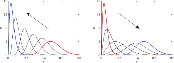
Figure 1: The left panel shows the result of switching $\gamma=0.5\to 0.05$, the right panel $\gamma=0.05\to 0.5$, both at fixed $\epsilon=1$ and $D=0.02$. The initial (red) and final (blue) gamma distributions are shown as heavy lines. The four intermediate lines are when the time-dependent solutions have $\langle x\rangle=0.1,\ 0.2,\ 0.3,\ 0.4$. The arrows are a reminder of the direction of motion, inward on the left and outward on the right.

Figure 2 shows how $\langle x\rangle$, ${\cal E}$ and ${\cal L}$ vary as functions of time, for the three values $D=0.01,\ 0.02,\ 0.04$. For $\langle x\rangle$ the movement from 0.5 to 0.05 is somewhat slower than the reverse process, but both processes occur on a similar timescale, and both are essentially independent of $D$. This is in contrast with other Fokker-Planck systems where the magnitude of the diffusion coefficient can have a very strong influence on the equilibration timescales KH17 ; Entropy .

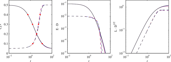
Figure 2: The first panel shows $\langle x\rangle$ as a function of time, the second panel shows ${\cal E}\cdot D$ (to indicate the ${\cal E}\sim D^{-1}$ scaling), and the third panel shows ${\cal L}\cdot D^{1/2}$ (to indicate the ${\cal L}\sim D^{-1/2}$ scaling). Solid lines denote $\gamma=0.5\to 0.05$, dashed lines the reverse. Each solid or dashed ‘line’ is in fact three – occasionally barely distinguishable – lines with $D=0.01,\ 0.02,\ 0.04$. The dots on the $\langle x\rangle$ curves correspond to the PDFs shown in figure 1.

For $\cal E$ and $\cal L$ the equilibration is again somewhat slower for $\gamma=0.5\to 0.05$ than the reverse. We can further identify clear scalings ${\cal E}\sim D^{-1}$ and ${\cal L}\sim D^{-1/2}$. Finally, $\cal L$ is greater for $\gamma=0.5\to 0.05$ than the reverse. These results are all understandable in terms of the interpretation of $\cal L$ as the number of statistically distinguishable states that the PDF evolves through: First, we recall from figure 1 that $\gamma=0.5\to 0.05$ had consistently narrower PDFs than the reverse. Narrower PDFs means more distinguishable states, hence larger $\cal L$ for $\gamma=0.5\to 0.05$ than the reverse. The ${\cal L}\sim D^{-1/2}$ scaling has the same explanation; smaller $D$ yields narrower PDFs, hence larger $\cal L$.

The first panel in figure 3 shows the previous quantities $\langle x\rangle$ and ${\cal L}\cdot D^{1/2}$, but now plotted against each other rather than separately against time. The behaviour is exactly as one might expect, with $\cal L$ growing more or less linearly with distance from the initial position. The right panel in figure 3 shows the entropy (16), again as a function of $\langle x\rangle$ rather than time, to emphasize the cyclic nature of the two processes. The significance is indeed as claimed above, with more localized PDFs having smaller entropy values. Note how $\gamma=0.5\to 0.05$, which had the narrower PDFs, has lower entropy values than the reverse process. Note also how reducing $D$ by a factor of two, thereby making the PDFs narrower, causes the entire cyclic pattern to shift downward by an essentially constant amount.

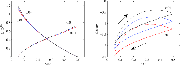
Figure 3: The left panel shows ${\cal L}\cdot D^{1/2}$, the right panel entropy, both as functions of $\langle x\rangle$. Solid lines denote $\gamma=0.5\to 0.05$, dashed lines the reverse. Numbers besides curves indicate $D=0.01,\ 0.02,\ 0.04$. The arrows on the entropy plot are a reminder of the direction of inward/outward motion.

Figure 4 shows how the standard deviation, skewness and kurtosis behave, again as functions of $\langle x\rangle$ throughout the two processes. The heavy green lines also show the behaviour that would be expected if the time-dependent PDFs were always gamma distributions throughout their evolution. That is, if gamma distributions have $\langle x\rangle=\gamma$, $\sigma=\sqrt{\gamma D}$, skewness$\;=2\sqrt{D/\gamma}$ and kurtosis$\;=6D/\gamma$ (setting $\epsilon=1$), then expressed as function of $\langle x\rangle$ we would have $\sigma/D^{1/2}=\sqrt{\langle x\rangle}$, (skewness$\,/\sqrt{D})=2/\sqrt{\langle x\rangle}$ and (kurtosis$\,/D)=6/{\langle x\rangle}$. As we can see, the $\gamma=0.5\to 0.05$ process follows these functional relationships reasonably well (especially for skewness and kurtosis), but for $\gamma=0.05\to 0.5$ all three quantities deviate substantially.

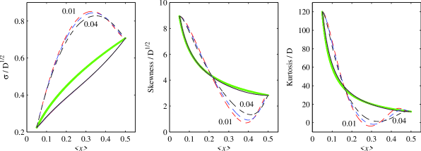
Figure 4: $\sigma/D^{1/2}$, (skewness$\,/D^{1/2}$) and (kurtosis$\,/D$), as functions of $\langle x\rangle$. Solid lines denote $\gamma=0.5\to 0.05$, dashed lines the reverse. Numbers besides curves indicate $D=0.01,\ 0.02,\ 0.04$. The heavy green curves are $\sqrt{\langle x\rangle}$, $2/\sqrt{\langle x\rangle}$ and $6/{\langle x\rangle}$, respectively, and indicate the behaviour expected for exact gamma distributions.

Further evidence of significant deviations from gamma distribution behaviour is seen in figure 5, showing the difference (13) directly. As expected from figure 4, $\gamma=0.05\to 0.5$ has a much greater difference than $\gamma=0.5\to 0.05$. The second and third panels show how the PDFs compare with the equivalent gamma distributions having the same $\langle x\rangle$ and $\sigma$ values as the actual PDFs at that instant. The differences are clearly visible, especially for $\gamma=0.05\to 0.5$, but also for $\gamma=0.5\to 0.05$.

Figure 5: The first panel shows the difference (13) between the actual PDF and the equivalent gamma distribution, as functions of $\langle x\rangle$. Solid lines denote $\gamma=0.5\to 0.05$, dashed lines the reverse, with arrows also indicating the direction of motion. The dots at $\langle x\rangle=0.3$ for $\gamma=0.05\to 0.5$, and $\langle x\rangle=0.1$ for $\gamma=0.5\to 0.05$, correspond to the other two panels: Panel 2 compares the $\gamma=0.05\to 0.5$ PDF with its equivalent gamma distribution; Panel 3 compares the $\gamma=0.5\to 0.05$ PDF with its equivalent gamma distribution. The actual PDFs in each case are solid (red), and the equivalent gamma distributions are dashed (blue). $D=0.04$ for both sets.

IV.2 $D>\gamma$

We next consider the case $D>\gamma$, where we demonstrated above that stationary solutions cannot exist at all, because the time-dependent PDF can only ever get closer and closer to the gamma distribution singularity at the origin, but can never actually achieve it. To explore what does happen in this case then, we simply repeat the above procedure, except that there is now only an ‘inward’ process, and no reverse. That is, instead of $\gamma=0.5\to 0.05$, let us consider $\gamma=0.5\to 0$. (Throughout this section we will also take $D=10^{-3}$, to facilitate comparison with results in the next section. For $\gamma=0$ of course any $D$ is greater than $\gamma$.)

Figure 6 shows the resulting PDFs, and how they approach ever closer to the origin, but never actually achieve the $x^{-1}$ blowup that would be implied by Eq. (4) for $a=\gamma/D=0$. The peak amplitude simply increases indefinitely, as $t^{1/2}$. The widths correspondingly also decrease; the apparent increase is an illusion caused by the logarithmic scale for $x$. The dashed lines also show the equivalent gamma distributions, as before. Note how the difference becomes increasingly noticeable; in line with the fact that the equivalent gamma distribution is tending toward its singular behaviour as $\langle x\rangle$ decreases, but the actual PDFs must always have $p(0)=0$.

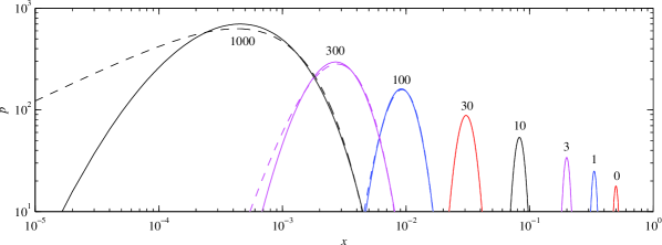
Figure 6: The initial condition is a gamma distribution with $\gamma=0.5$, $\epsilon=1$ and $D=10^{-3}$; $\gamma$ is then switched to 0, and the solution is evolved according to Eq. (3). Numbers besides curves indicate time, from the initial condition at $t=0$ to the final time 1000. The dashed curves indicate the equivalent gamma distributions having the same $\langle x\rangle$ and $\sigma$.

Figure 7 is the equivalent of figure 2, and directly compares $\gamma=0.5\to 0$ here with the previous $\gamma=0.5\to 0.05$. We see that $\langle x\rangle$ starts out very similarly, but instead of equilibrating to 0.05, it now tends to 0 as $t^{-1}$. $\cal E$ again starts out similarly, but ultimately tends to 0 much slower, as $t^{-3}$ instead of exponentially. This $t^{-3}$ scaling for $\cal E$ has an interesting consequence for $\cal L$, namely that $\cal L$ does saturate to a finite value ${\cal L}_{\infty}$ (since $\int t^{-3/2}\,dt$ remains bounded for $t\to\infty$) even though the PDF itself never settles to a stationary state.

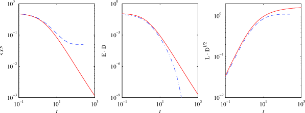
Figure 7: As in figure 2, the first panel shows $\langle x\rangle$, the second panel shows ${\cal E}\cdot D$, and the third panel ${\cal L}\cdot D^{1/2}$. Solid lines denote $\gamma=0.5\to 0$ for $D=10^{-3}$, dashed lines the previous $\gamma=0.5\to 0.05$ for $D=0.01$. Note how the scalings of $\cal E$ and $\cal L$ with $D$ are still preserved even when $D$ is changed by a factor of 10.

Figure 8 shows entropy, $\sigma$, skewness and kurtosis, so some of the results as in figures 3 and 4. Entropy and $\sigma$ are again both good measures of how narrow the PDF is, becoming ever smaller as the peak moves toward the origin. Skewness and kurtosis seem to follow the expected gamma distribution relationship extremely well, even though we saw before in figure 6 that the PDFs are actually different from gamma distributions. As $\langle x\rangle\to 0$, both skewness and kurtosis thus become indefinitely large.

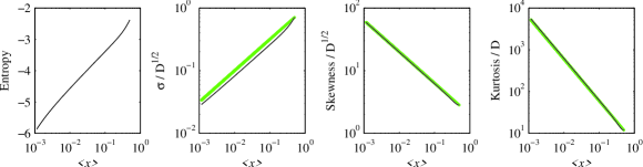
Figure 8: Entropy, $\sigma/D^{1/2}$, (skewness$\,/D^{1/2}$) and (kurtosis$\,/D$), as functions of $\langle x\rangle$, for the $\gamma=0.5\to 0$ calculation from figure 6. The heavy green curves in the last three panels are $\sqrt{\langle x\rangle}$, $2/\sqrt{\langle x\rangle}$ and $6/{\langle x\rangle}$, respectively, and indicate the behaviour expected for exact gamma distributions.

IV.3 $Q\neq 0$

Finally, we turn to the Fokker-Planck equation (11) with additive noise included, and use it to explore the two questions that could not be addressed otherwise. First, how does a process like $\gamma=0.5\to 0$ then equilibrate to a stationary solution? Second, what does the reverse process $\gamma=0\to 0.5$ look like?

We will keep $D=10^{-3}$ and $Q=10^{-5}$ fixed throughout this section. Since the effective diffusion coefficients in (11) are $Dx^{2}$ and $Q$ [recall also the denominator of Eq. (12)], this means that $Q$ is dominant only within $x\leq 0.1$; any stationary solutions with peaks much beyond that are effectively pure gamma distributions.

Figure 9 shows the same type of inward/outward process as before in figure 1, only now switching $\gamma$ between 0.5 and 0.1. Comparing with figure 1, we see that the dynamics are very similar, just with all the peaks considerably narrower, which is to be expected if $D=10^{-3}$ rather than 0.02. The only other point to note is how the final peak in the left panel is lower than the previous peak at $\langle x\rangle=0.2$, which is different from figure 1, where $\gamma=0.5\to 0.05$ had peaks monotonically increasing throughout the entire evolution. The reason the final peak here decreases slightly is precisely the influence of $Q$ in this region; if this peak is now seeing just as much diffusion from $Q$ as from $D$, it is not surprising that it spreads out somewhat more, and is correspondingly somewhat lower than a pure gamma distribution would be.

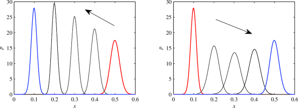
Figure 9: The left panel shows the result of switching $\gamma=0.5\to 0.1$, the right panel $\gamma=0.1\to 0.5$, both at fixed $\epsilon=1$, $D=10^{-3}$ and $Q=10^{-5}$. The initial (red) and final (blue) gamma distributions are shown as heavy lines. The three intermediate lines are when the time-dependent solutions have $\langle x\rangle=0.2,\ 0.3,\ 0.4$. ${\cal L}_{\infty}=25$ on the left and 16 on the right.

Figure 10 shows the fundamentally new case, namely switching $\gamma$ between 0.5 and 0. The inward process $\gamma=0.5\to 0$ is again very similar to either figure 1 or 9. The only difference to figure 6 is that the process does actually equilibrate to a stationary solution now, as given by Eq. (12). The reverse process $\gamma=0\to 0.5$ is rather different though. The initial central peak now broadens far more than previously seen in figures 1 and 9.

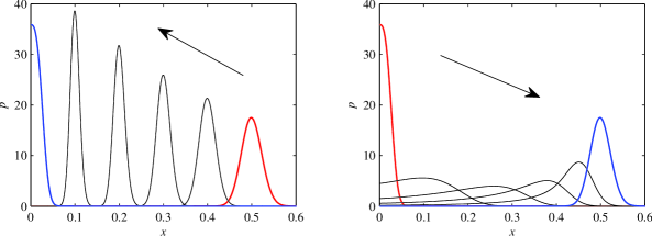
Figure 10: The left panel shows the result of switching $\gamma=0.5\to 0$, the right panel $\gamma=0\to 0.5$, both at fixed $\epsilon=1$, $D=10^{-3}$ and $Q=10^{-5}$. The initial (red) and final (blue) gamma distributions are shown as heavy lines. The four intermediate lines are when the time-dependent solutions have $\langle x\rangle=0.1,\ 0.2,\ 0.3,\ 0.4$. ${\cal L}_{\infty}=35$ on the left and 9.5 on the right.

One interesting consequence of this extreme broadening for $\gamma=0\to 0.5$ is on the total information length ${\cal L}_{\infty}$. In figure 9 these values are 25 and 16, respectively, whereas in figure 10 they are 35 and 9.5. That is, in both cases decreasing $\gamma$ yields larger ${\cal L}_{\infty}$ values than increasing $\gamma$ does, consistent with the peaks being narrower, and hence passing through more statistically distinguishable states. Next, comparing 25 for $\gamma=0.5\to 0.1$ versus 35 for $\gamma=0.5\to 0$, this is exactly as one might expect: having the peak travel somewhat further yields extra information length. However, comparing 16 for $\gamma=0.1\to 0.5$ versus 9.5 for $\gamma=0\to 0.5$ is puzzling then! The peak has further to travel, but accomplishes it with less information length. The reason is precisely this extreme broadening, which substantially reduces the number of distinguishable states along the way. See also KH17 ; Entropy , where the same effect was studied for Gaussian PDFs, and values of $D$ as small as $10^{-7}$, leading to fundamentally different scalings of ${\cal L}_{\infty}$ with $D$ for inward and outward processes.

Returning to the central question of this paper, namely how close the time-dependent PDFs are to gamma distributions, the results for figure 9 are similar to the previous ones. In particular, we recall that before in figure 5 we had the difference scaling as $D^{1/2}$, so a smaller $D$ here means a smaller difference. These results are approaching the small $D$ regime where gamma distributions become very close to Gaussians anyway, which generally remain close to Gaussian as they move.

However, for the $\gamma=0\to 0.5$ process in figure 10, the intermediate stages do not look much like gamma distributions. (The final equilibrium is indistinguishable from a gamma distribution though, consistent with $Q$ being completely negligible for these values of $x$.) For the intermediate stages, these were found to be so different from gamma distributions that attempting to fit a gamma distribution having the same $\langle x\rangle$ and $\sigma$ made little sense; this extreme broadening and long tail trailing behind the peak meant that both $\langle x\rangle$ and $\sigma$ were too different from the normal expectation that they should be measures of ‘peak’ and ‘width’.

Instead, we simply asked the question, which values of $a$ and $b$ would minimize the quantity $\int|p-p_{\rm bf}|\,dx$, where $p$ is the time-dependent PDF to be fitted, and $p_{\rm bf}$ is the best-fit gamma distribution. Unlike our previous difference formula, this does not yield simple analytic formulas for the $a$ and $b$ to choose, but is numerically still straightforward to implement. Figure 11 shows the results, for two of the intermediate stages in the $\gamma=0\to 0.5$ process. We can see that the fit is rather poor, indicating that these PDFs are significantly different from gamma distributions.

This misfit is also not caused by the inclusion of $Q$; if this or any similar central peak is evolved for either small or zero $Q$ in the Fokker-Planck equation, the result is always similar to here. As explained also in KH17 ; Entropy , the dynamics of how central peaks move away from the origin is simply different from how peaks already away from the origin move, regardless of whether the final states are Gaussians as in KH17 ; Entropy , or gamma distributions as here.

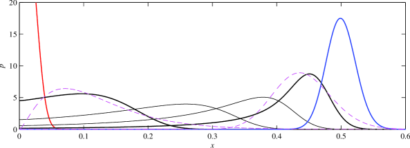
Figure 11: The $\gamma=0\to 0.5$ process as in figure 10, but now shown in more detail. The dashed (magenta) curves are the gamma distributions that best fit the two thicker curves at intermediate times. Note how even a ‘best-fit’ is a rather poor approximation to the actual PDFs.

V Conclusion

Gamma distributions are among the most popular choices for modelling a broad range of experimentally determined PDFs. It is often assumed that time-dependent PDFs can then simply be modelled as gamma distributions with time-varying parameters $a$ and $b$. In this work we have demonstrated that one should be cautious with such an approach. By numerically solving the full time-dependent Fokker-Planck equation, we found that there are three sets of circumstances where the PDFs can differ significantly from gamma distributions:

• If $D<\gamma$, so that stationary solutions exist, but $D$ is also sufficiently close to $\gamma$ that a gamma distribution differs significantly from a Gaussian, then the time-dependent PDFs will also differ significantly from gamma distributions.

• If $D>\gamma$, stationary gamma distributions do not exist at all. Instead, peaks move ever closer to the origin, and in the process increasingly differ from gamma distributions.

• If the initial condition is a peak right on the origin – either as a result of adding additive noise to produce stationary solutions even for $D>\gamma$, or simply as an arbitrary initial condition – then any evolution away from the origin will differ significantly from gamma distributions. Unlike the previous two items, which become more pronounced for larger $D$, this effect is most clearly visible for smaller $D$, where the mismatch between the naturally narrower peaks and the extreme broadening seen in figure 11 becomes increasingly significant.

In summary, our results show that a simple Langevin equation model mimics the strong fluctuations of far-from-equilibrium systems. This model has gamma distributions as steady-state solutions, but the time-dependent solutions can deviate considerably from this law. This makes tasks such as Bayesian and frequentist inference of the model from data more complicated. On the other hand, the model shows complex asymptotic dynamics with situations when a steady state is reached or not, different from the one of the deterministic logistic model that invariably evolves to the maximum capacity. The studied model is general enough and can be applied to many practical situations in biology, economics, finance, and physics. Future work will apply some of these ideas to fitting actual data.

Appendix A Derivation of the Fokker-Planck Equations

In order to derive the Fokker-Planck equation (3) from the Langevin equation (1), it is useful to introduce a generating function $Z$:

$$Z=e^{i\lambda x(t)}.$$ (19)

Then, by definition of ‘average’, the average of $Z$ is related to the PDF, $p(x,t)$, as

$$\langle Z\rangle=\int dx\,Z\,p(x,t)=\int dx\,e^{i\lambda x(t)}\,p(x,t).$$ (20)

Thus, we see that $\langle Z\rangle$ is the Fourier transform of $p(x,t)$. The inverse Fourier transform of $\langle Z\rangle$ then gives $p(x,t)$:

$$p(x,t)=\frac{1}{2\pi}\int d\lambda\,e^{-i\lambda x}\,\langle Z\rangle.$$ (21)

We note that Eq. (21) can be written as

$$p(x,t)=\left\langle\frac{1}{2\pi}\int d\lambda\,e^{i\lambda(x-x(t))}\right\rangle=\left\langle\delta(x-x(t))\right\rangle,$$ (22)

which is another form of $p(x,t)$. To obtain the equation for $p(x,t)$, we first derive the equation for $\langle x\rangle$ and then take the inverse Fourier transform as summarised in the following.

We differentiate $Z$ with respect to time $t$ and use Eq. (1) to obtain

$$\partial_{t}Z=i\lambda\partial_{t}xZ=i\lambda(\gamma x-\epsilon x^{2}+\xi(t)x)Z=\lambda\left[\gamma\partial_{\lambda}+i\epsilon\partial_{\lambda\lambda}+\xi\partial_{\lambda}\right]Z,$$ (23)

where $xZ=-i\partial_{\lambda}Z$ was used. The formal solution to Eq. (23) is

$$Z(t)=\lambda\int dt_{1}\,\left[\gamma\partial_{\lambda}+i\epsilon\partial_{\lambda\lambda}+\xi(t_{1})\partial_{\lambda}\right]Z(t_{1}).$$ (24)

The average of Eq. (23) gives

$$\partial_{t}\langle Z\rangle=\lambda(\gamma\partial_{\lambda}+i\epsilon\partial_{\lambda\lambda})\langle Z\rangle+\lambda\langle\xi(t)\partial_{\lambda}Z(t)\rangle.$$ (25)

To find $\langle\xi(t)\partial_{\lambda}Z(t)\rangle$, we use Eq. (24) iteratively as follows:

$$\langle\xi(t)\partial_{\lambda}Z\rangle = \left\langle\xi(t)\partial_{\lambda}\left[\lambda\int dt_{1}\,\left[\gamma\partial_{\lambda}+i\epsilon\partial_{\lambda\lambda}+\xi(t_{1})\partial_{\lambda}\right]Z(t_{1})\right]\right\rangle$$ (26)

$$= \langle\xi(t)\rangle\partial_{\lambda}\left[\lambda\int dt_{1}\,\left[\gamma\partial_{\lambda}+i\epsilon\partial_{\lambda\lambda}\right]\langle Z(t_{1})\rangle\right]+\partial_{\lambda}\left[\lambda\int dt_{1}\,\langle\xi(t)\xi(t_{1})\rangle\partial_{\lambda}\langle Z(t_{1})\rangle\right]$$

$$= \partial_{\lambda}\Bigl{[}\lambda\left[D\partial_{\lambda}\langle Z(t)\rangle\right]\Bigr{]}.$$

Here we used the independence of $\xi(t)$ and $Z(t_{1})$ for $t_{1}<t$, $\langle\xi(t)Z(t_{1})\rangle=\langle\xi(t)\rangle\langle Z(t_{1})\rangle=0$, together with Eq. (2), $\int_{0}^{t}dt_{1}\,\delta(t-t_{1})={1}/{2}$, and $\langle\xi\rangle=0$. By substituting Eq. (26) into Eq. (25) we obtain

$$\partial_{t}\langle Z\rangle=\lambda(\gamma\partial_{\lambda}+i\epsilon\partial_{\lambda\lambda})\langle Z\rangle+\lambda\partial_{\lambda}\Bigl{[}\lambda\left[D\partial_{\lambda}\langle Z(t)\rangle\right]\Bigr{]}.$$ (27)

The inverse Fourier transform of Eq. (27) then gives us

$$\frac{\partial}{\partial t}\,p(x,t)=-\frac{\partial}{\partial x}\Bigl{[}(\gamma x-\epsilon x^{2})p(x,t)\Bigr{]}+D\,\frac{\partial}{\partial x}\left[x\,\frac{\partial}{\partial x}\Bigl{[}x\,p(x,t)\Bigr{]}\right]$$ (28)

which is Eq. (3). Specifically, the inverse Fourier transforms of the first and last terms in Eq. (27) are shown explicitly in the following:

$$\frac{1}{2\pi}\int d\lambda\,e^{-i\lambda x}\langle\partial_{t}Z\rangle=\partial_{t}\left[\frac{1}{2\pi}\int d\lambda\,e^{-i\lambda x}\langle Z\rangle\right]=\frac{\partial}{\partial t}\,p(x,t),$$ (29)

$$\frac{D}{2\pi}\int d\lambda\,e^{-i\lambda x}\lambda\partial_{\lambda}\left[\lambda\partial_{\lambda}\langle Z\rangle\right]=D\,\frac{\partial}{\partial x}\left[x\,\frac{\partial}{\partial x}\Bigl{[}x\,p(x,t)\Bigr{]}\right],$$ (30)

where integration by parts was used twice in obtaining Eq. (30). The additional $Q\partial_{xx}p$ term in the Fokker-Planck equation (11) can be derived in the same way.

Appendix B Time-dependent Analytical Solutions of Eq. (3)

We begin by making the change of variables $y=1/x$ in Eq. (1) to obtain

$$\frac{dy}{dt}=-(\gamma+\xi)y+\epsilon.$$ (31)

By using the Stratonovich calculus Klebaner ; Gardiner ; WongZakai , the solution to Eq. (31) is found as

$$y(t)=y_{0}e^{-(\gamma t+B(t))}+\epsilon e^{-(\gamma t+B(t))}\int_{0}^{t}dt_{1}e^{(\gamma t_{1}+B(t_{1}))},$$ (32)

where $y_{0}=y(t=0)$ and $B(t)=\int_{0}^{t}\,dt_{1}\,\xi(t_{1})$ is the Brownian motion. Therefore,

$$x(t)=\frac{x_{0}e^{\gamma t+B(t)}}{1+\epsilon x_{0}\int_{0}^{t}dt_{1}e^{(\gamma t_{1}+B(t_{1}))}},$$ (33)

where $x_{0}=x(t=0)$. In Eq. (33), $e^{B(t)}$ is the geometric Brownian motion while $e^{-\gamma t-B(t)}$ is the geometric Brownian motion with a drift (e.g. Klebaner ). The time integral of the latter is used in understanding stochastic processes in financial mathematics and many other areas bertoin ; matsumoto . In particular, in the long time limit, its PDF can be shown to be a gamma distribution. However, this PDF of $x$ is not particularly useful as it involves complicated summations and integrals that cannot be evaluated in closed form bertoin ; matsumoto .

References

- (1) H. Risken, The Fokker-Planck Equation: Methods of Solution and Applications (Springer, 1996).
- (2) F. Klebaner, Introduction to Stochastic Calculus with Applications (Imperial College Press, 2012).
- (3) C. Gardiner, Stochastic Methods, 4th Ed., Chapter 4.4 (Springer, 2008).
- (4) E.-W. Saw, D. Kuzzay, D. Faranda, A. Guittonneau, F. Daviaud, C. Wiertel-Gasquet, V. Padilla and B. Dubrulle, Experimental characterization of extreme events of inertial dissipation in a turbulent swirling flow, Nat. Commun. 7:12466 doi: 10.1038/ncomms12466 (2016).
- (5) E. Kim and P.H. Diamond, On intermittency in drift wave turbulence: structure of the probability distribution function, Phys. Rev. Lett. 88, 225002 (2002)
- (6) E. Kim and P.H. Diamond, Zonal flows and transient dynamics of the L-H transition, Phys. Rev. Lett. 90, 185006 (2003).
- (7) E. Kim, Consistent theory of turbulent transport in two dimensional magnetohydrodynamics, Phys. Rev. Lett. 96, 084504 (2006).
- (8) E. Kim and J. Anderson, Structure-based statistical theory of intermittency, Phys. Plasmas 15, 114506 (2008).
- (9) A.P.L. Newton, E. Kim and H.-L. Liu, On the self-organizing process of large scale shear flows, Phys. Plasmas 20, 092306 (2013).
- (10) K. Srinivasan and W.R. Young, Zonostrophic Instability, J. Atmos. Sci. 69, 1633 (2012).
- (11) K.M. Sayanagi, A.P. Showman and T.E. Dowling, The emergence of multiple robust zonal jets from freely evolving, three-dimensional stratified geostrophic turbulence with applications to Jupiter, J. Atmos. Sci. 65, 12 (2008).
- (12) M. Tsuchiya, A. Giuliani, M. Hashimoto, J. Erenpreisa and K. Yoshikawa, Emergent Self-Organized Criticality in Gene Expression Dynamics: Temporal Development of Global Phase Transition Revealed in a Cancer Cell Line, PLoS One 10, e0128565 (2015).
- (13) C. Tang and P. Bak, Mean field theory of self-organized critical phenomena, J. Stat. Phys. 51, 797 (1988).
- (14) H.J. Jensen, Self-organized Criticality: Emergent Complex Behavior in Physical and Biological Systems (Cambridge Univ. Press, 1998).
- (15) G. Pruessner, Self-organised Criticality (Cambridge Univ. Press, 2012).
- (16) G. Longo and M. Montévil, From physics to biology by extending criticality and symmetry breaking, Progress in Biophysics and Molecular Biology: Systems Biology and Cancer 106, 340 (2011).
- (17) S.W. Flynn, H.C. Zhao, and J.R. Green, Measuring disorder in irreversible decay processes, J. Chem. Phys. 141, 104107 (2014)
- (18) J.W. Nichols, S.W. Flynn and J.R. Green, Order and disorder in irreversible decay processes, J. Chem. Phys. 142, 064113 (2015).
- (19) M.L. Ferguson, D. Le Coq, M. Jules, S. Aymerich, O. Radulescu, N. Declerck and C.A. Royer, Reconciling molecular regulatory mechanisms with noise patterns of bacterial metabolic promoters in induced and repressed states, PNAS 109, 155 (2012).
- (20) V. Shahrezaei and P. S. Swain, Analytical distributions for stochastic gene expression, PNAS 105 (45) 17256 (2008).
- (21) R. Thomas, L.Torre, X. Chang and S. Mehrotra, Validation and characterization of DNA microarray gene expression data distribution and associated moments, Bioinformatics 11, 576 (2010).
- (22) S. Iyer-Biswas, F. Hayot, and C. Jayaprakash, Stochasticity of gene products from transcriptional pulsing, Phys. Rev. E 79, 031911 (2009).
- (23) V. Elgart, T. Jia, A.T. Fenley and R. Kulkarni, Connecting protein and mRNA burst distributions for stochastic models of gene expression, Physical Biology 8, 046001 (2011).
- (24) Delbrück, M, The burst size distribution in the growth of bacterial viruses (bacteriophages), J. Bacteriology 50, 131 (1945).
- (25) M. Delbrück, Statistical fluctuations in autocatalytic reactions, J. Chem. Phys. 8, 120 (1940).
- (26) I. G. de Jong, P. Haccou and O.P Kuipers, Bet hedging or not? A guide to proper classification of microbial survival strategies, Bioessays 33, 215 (2011).
- (27) N. Balaban, J. Merrin, R. Chait, L. Kowalik and S. Leibler, Bacterial persistence as a phenotypic switch, Science 305, 1622 (2004).
- (28) E. Kim, H. Liu and J. Anderson, Probability distribution function for self-organization of shear flows, Phys. Plasmas 16, 052304 (2009).
- (29) E. Kim and R. Hollerbach, Time-Dependent Probability Density Function in Cubic Stochastic Processes, Phys. Rev. E 94, 052118 (2016).
- (30) P. Glansdorff and I. Prigogine, Thermodynamic Theory of Structure, Stability and Fluctuations (Wiley, 1971).
- (31) M. Suzuki, Microscopic theory of formation of macroscopic order, Phys. Lett. A 75, 331 (1980).
- (32) M. Suzuki, The variational theory and rate equation method with applications to relaxation near the instability point, Physica A 105, 631 (1981).
- (33) J.S. Langer, M. Baron and H.D. Miller, New computational method in the theory of spinodal decomposition, Phys. Rev. A. 11, 1417 (1975).
- (34) Y. Saito, Relaxation in a Bistable System, J. Phys. Soc. Japan 61, 388 (1976).
- (35) H. Hasegawa, Variational Approach in Studies with Fokker-Planck Equations, Prog. Theor. Phys. 58, 128 (1977).
- (36) B. Dennis and R. F. Costantino, Analysis of steady-state populations with the gamma abundance model: application to Tribolium, Ecology 69, 1200 (1988).
- (37) H.-Y. Liao, B.-Q. Ai and L. Hu, Effects of multiplicative colored noise on bacteria growth, Braz. J. Phys. 37, 1125 (2007).
- (38) E. Wong and M. Zakai, On the convergence of ordinary integrals to stochastic integrals, Ann. Math. Stat. 36, 1560 (1960).
- (39) S.C. Bagui and K.L. Mehra, Convergence of Binomial, Poisson, Negative-Binomial, and Gamma to Normal Distribution: Moment Generating Functions Technique, Am. J. Math. Stat. 6, 115 (2016).
- (40) E. Kim and R. Hollerbach, Geometric structure and information change in phase transitions, Phys. Rev. E 95, 022137 (2017).
- (41) R. Hollerbach and E. Kim, Information geometry of non-equilibrium processes in a bistable system with a cubic damping, Entropy 19, 268 (2017).
- (42) L.-M. Tenkès, R. Hollerbach and E. Kim, Time-dependent probability density functions and information geometry in stochastic logistic and Gompertz models, arXiv:1708.02789
- (43) B.R. Frieden, Physics from Fisher Information (Cambridge Univ. Press, 2000).
- (44) W.K. Wootters, Statistical Distance and Hilbert Space, Phys. Rev. D, 23, 357 (1981).
- (45) S.B. Nicholson and E. Kim, Phys. Lett. A. 379, 8388 (2015).
- (46) S.B. Nicholson and E. Kim, Structures in sound: Analysis of Classical Music Using the Information Length, Entropy 18, 258, e18070258 (2016).
- (47) J. Heseltine and E. Kim, Novel mapping in a non-equilibrium stochastic process, J. Phys. A 49, 175002 (2016).
- (48) E. Kim, U. Lee, J. Heseltine and R. Hollerbach, Geometric structure and geodesic motion in a solvable model of non-equilibrium stochastic process, Phys. Rev. E 93, 062127 (2016).
- (49) J. Bertoin and M. Yor, Exponential functionals of L vy processes, Prob. Surveys, 2, 191 (2005).
- (50) H. Matsumoto and M. Yor, Exponential functionals of Brownian motion, I: Probability laws at fixed time, Prob. Surveys, 2 312 (2005).