Online Service with Delay

Abstract

In this paper, we introduce the online service with delay problem. In this problem, there are $n$ points in a metric space that issue service requests over time, and a server that serves these requests. The goal is to minimize the sum of distance traveled by the server and the total delay in serving the requests. This problem models the fundamental tradeoff between batching requests to improve locality and reducing delay to improve response time, that has many applications in operations management, operating systems, logistics, supply chain management, and scheduling.

Our main result is to show a poly-logarithmic competitive ratio for the online service with delay problem. This result is obtained by an algorithm that we call the preemptive service algorithm. The salient feature of this algorithm is a process called preemptive service, which uses a novel combination of (recursive) time forwarding and spatial exploration on a metric space. We hope this technique will be useful for related problems such as reordering buffer management, online TSP, vehicle routing, etc. We also generalize our results to $k>1$ servers.

1 Introduction

Suppose there are $n$ points in a metric space that issue service requests over time, and a server that serves these requests. A request can be served at any time after it is issued. The goal is to minimize the sum of distance traveled by the server (service cost) and the total delay of serving requests (delay of a request is the difference between the times when the request is issued and served). We call this the online service with delay (osd) problem. To broaden the scope of the problem, for each request we also allow any delay penalty that is a non-negative monotone function of the actual delay, the penalty function being revealed when the request is issued. Then, the goal is to minimize the sum of service cost and delay penalties.

This problem captures many natural scenarios. For instance, consider the problem of determining the schedule of a technician attending service calls in an area. It is natural to prioritize service in areas that have a large number of calls, thereby balancing the penalties incurred for delayed service of other requests with the actual cost of dispatching the technician. In this context, the delay penalty function can be loosely interpreted as the level of criticality of a request, and different requests, even at the same location, can have very different penalty functions. In general, the osd problem formalizes the tradeoff between batching requests to minimize service cost by exploiting locality and quick response to minimize delay or response time. Optimizing this tradeoff is a fundamental problem in many areas of operations management, operating systems, logistics, supply chain management, and scheduling.

A well-studied problem with a similar motivation is the reordering buffer management problem [48, 32, 41, 31, 35, 7, 2, 16, 8, 6] — the only difference with the osd problem is that instead of delay penalties, there is a cap on the number of unserved requests at any time. Thus, the objective only contains the service cost, and the delays appear in the constraint. A contrasting class of problems are the online traveling salesman problem and its many variants [38, 45, 11, 4, 5], where the objective is only defined on the delay (average/maximum completion time, number of requests serviced within a deadline, and so on), but the server’s movement is constrained by a given speed (which implies that there are no competitive algorithms for delay in general, so these results restrict the sequence or the adversary in some manner). In contrast to these problem classes, both the service cost and the delay penalties appear in the objective of the osd problem. In this respect, the osd problem bears similarities to the online multi-level aggregation problem [42, 18, 21], where a server residing at the root of a tree serves requests arriving online at the leaves after aggregating them optimally. While these problems are incomparable from a technical perspective, all of them represent natural abstractions of the fundamental tradeoff that we noted above, and the right abstraction depends on the specific application.

Our main result is a a poly-logarithmic competitive ratio for the osd problem in general metric spaces.

Theorem 1.

There is a randomized algorithm with a competitive ratio of $O(\log^{4}n)$ for the osd problem.

Before proceeding further, let us try to understand why the osd problem is technically interesting. Recall that we wish to balance service costs with delay penalties. Consider the following natural algorithm. Let us represent the penalty for all unserved requests at a location as a “ball” growing out of this location. These balls collide with each other and merge, and grow further together, until they reach the server’s current location. At this point, the server moves and serves all requests whose penalty balls reached it. Indeed, this algorithm achieves the desired balance — the total delay penalty is equal (up to constant factors) to the total service cost. But, is this algorithm competitive against the optimal solution? Perhaps surprisingly, it is not!

Consider the instance in Fig. 1 on a star metric, where location $p_{0}$ is connected to the center with an edge of length $W$ ($\gg 1$), but all other locations $p_{1},p_{2},\ldots,p_{n-1}$ are connected using edges of length 1. The delay penalty function for each request is a constant request-specific rate times the delay. All requests for locations $p_{i}$, $i\geq 1$ arrive at time $0$, with $p_{i}$ getting a single request accumulating waiting cost at rate $(W+1)^{i+1}$. Location $p_{0}$ is special in that it gets a request with an infinite rate at time $0$ and at all times $1/(W+1)^{i}$. For this instance, the algorithm’s server will move to location $p_{i}$ and back to $p_{0}$ at each time $1/(W+1)^{i}$. This is because the “delay ball” for $p_{i}$ reaches $p_{0}$ at time $1/(W+1)^{i}$, and the “delay ball” for $p_{0}$ instantly reaches $p_{i}$ immediately afterward. Note, however, that the “delay balls” of all locations $p_{j}$, $j<i$, have not crossed their individual edges connecting them to the center at this time. Thus, the algorithm incurs a total cost of $\Omega(nW)$. On the other hand, the optimal solution serves all the requests for $p_{1},p_{2},\ldots,p_{n-1}$ at time 0, moves to location $p_{0}$, and stays there the entire time. Then, the optimal solution incurs a total cost of only $O(n+W)$.

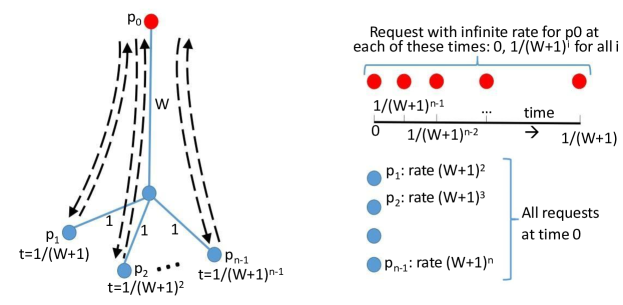
Figure 1: An example showing the inadequacy of simple balancing of delay penalties with service costs.

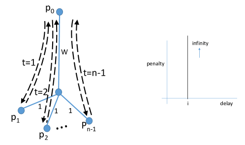
Figure 2: An example in which requests must be served preemptively even before incurring any delay penalty. The function on the right is the delay penalty function. The penalty is $0$ till delay $i$, at which point the penalty goes to infinity. Page $p_{i}$, for each $i\geq 1$, has a single request arriving at time $0$. Page $p_{0}$ has requests at times $0,1,2,\ldots,n-1$.

In this example, the algorithm must serve requests at $p_{1}$, $p_{2}$, $\ldots$, $p_{n}$ even when they have incurred a very small delay penalty. In fact, this example can be modified to create situations where requests that have not incurred any delay penalty at all need to be served! Consider the instance in Fig. 2 on the same star metric with different delay penalties. Note that the delay penalty enforces deadlines – a request for $p_{i}$ must incur delay $\leq i$. (Requests for $p_{0}$ must be served immediately.) On this instance, the “ball” growing algorithm moves to location $p_{i}$ and back to $p_{0}$ for each time $i\geq 0$, incurring a total cost of $\Omega(nW)$. On the other hand, the optimal solution serves all the requests for $p_{1},p_{2},\ldots,p_{n-1}$ immediately after serving the request for $p_{0}$ at time 0, and then stays at location $p_{0}$ for the entire remaining time, thereby incurring a total cost of only $O(n+W)$. In order to be competitive on this example, an osd algorithm must serve requests at $p_{1},p_{2},\ldots,p_{n}$ even before they have incurred any delay penalty.

This illustrates an important requirement of an osd algorithm — although it is trying to balance delay penalties and service costs, it cannot hope to do so “locally” for the set of requests at any single location (or in nearby locations, if their penalty balls have merged). Instead, it must perform “global” balancing of the two costs, since it has to serve requests that have not accumulated any delay penalty. This principle, that we call preemptive service, is what makes the osd problem both interesting and challenging from a technical perspective, and the main novelty of our algorithmic contribution will be in addressing this requirement. Indeed, we will call our algorithm the preemptive service algorithm (or ps algorithm).

As we will discuss later, a natural choice for preemptive service is to serve requests which will go critical the earliest. However, on more general metrics than a star, preemptive service must also consider the spatial locality of non-critical requests.

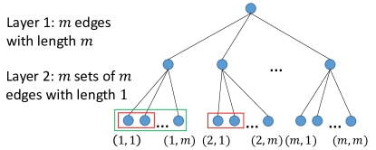
Figure 3: An example showing that spatial locality should be considered in preemptive service. The red boxes show a set of requests that might be served using budget $2m$ if spatial locality is not considered. The green box shows a set of requests that might be served using budget $2m$ if spatial locality is considered.

Consider a subtree where we would like to perform preemptive service (see Fig. 3). The subtree has two layers, with $m$ edges of length $m$ in the first layer. Each of these $m$ edges also has $m$ children that are connected by edge of length $1$. We use the pair $(i,j)$ to denote the $j$-th children of the $i$-th subtree. Each of these nodes have a request. Now suppose the ordering for these requests to become critical is $(1,1)$, $(2,1)$, $\dots$, $(m,1)$, $(1,2)$, $(2,2)$, $\dots$, $(m,2)$, $\dots$, $(m,m)$. If we have a budget of $2cm$ for the preemptive service for some $c<m$, we can only serve at most $2c$ requests if we follow the order in which they will become critical. The total cost for the entire tree would be $\Theta(m^{2})$. However we can choose to preemptively serve all requests in $c$ of the subtrees, and in this way we can finish preempting the whole tree for $O(m)$ cost.

osd on HSTs. Our main theorem (Theorem 1) is obtained as a corollary of our following result on an HST. A hierarchically separated tree (HST) is a rooted tree where every edge length is shorter by a factor of at least $2$ from its parent edge length.

Theorem 2.

There is a deterministic algorithm with a competitive ratio of $O(h^{3})$ for the osd problem on a hierarchically separated tree of depth $h$.

Theorem 1 follows from Theorem 2 by a standard probabilistic embedding of general metric spaces in HSTs of depth $O(\log n)$ with an expected distortion of $O(\log n)$ in distances:

Theorem 3.

For any $n$-point metric space $\cal M$, there exists a distribution $\cal D$ over HSTs of depth $O(\log n)$, such that the expected distortion is $O(\log n)$. In other words, for any two points $(u,v)$, the following holds:

$$d_{\cal M}(u,v)\leq{\mathbb{E}}_{T\sim{\cal D}}[d_{T}(u,v)]\leq O(\log n)d_{\cal M}(u,v),$$

where $d_{\cal M}(u,v)$ and $d_{T}(u,v)$ denote the distance between $u$ and $v$ in the metric space $\cal M$ and the HST $T$ respectively. The $n$ points in the metric space $\cal M$ are leaves in each of the HSTs in the distribution.

This is done in two steps. Define a $2$-HST as a rooted tree where every edge length is shorter by a factor of at exactly $2$ from its parent edge length. First, a well-known result of Fakcharoenphol et al. [33] states that any metric space can be embedded into a distribution over $2$-HSTs with distortion $O(\log n)$, where the points of the metric space are the leaves of the trees. The depth of the HSTs is, however, dependent on the aspect ratio of the metric space, i.e., the maximum ratio between distances of two pairs of points in $\cal M$. On the other hand, a result of Bansal et al. [13] (Theorem 8 of the paper) states that a $2$-HST with $n$ leaves can be deterministically embedded into an HST of height $O(\log n)$ with the same leaf set, such that the distance between any pair of leaves is distorted by at most $4$. The theorem follows by composing these two embeddings.

Note that Theorem 2 also implies $O(1)$ deterministic algorithms for the osd problem on the interesting special cases of the uniform metric and any star metric, since these are depth-1 HSTs.

Generalization to $k$ servers. We also generalize the osd problem to $k>1$ servers. This problem generalizes the well-known online paging (uniform metric), weighted paging (star metric), and $k$-server (general metric) problems. We obtain an analogous theorem to Theorem 2 on HSTs, which again extends to an analogous theorem to Theorem 1 on general metrics.

Theorem 4.

There is a deterministic algorithm with a competitive ratio of $O(kh^{4})$ for the $k$-osd problem on an HST of depth $h$. As immediate corollaries, this yields the following:

• A randomized algorithm with a competitive ratio of $O(k\log^{5}n)$ for the $k$-osd problem on general metric spaces.

• A deterministic algorithm with a competitive ratio of $O(k)$ for the unweighted and weighted paging problems with delay penalties, which are respectively special cases of $k$-osd on the uniform metric and star metrics.

Because of the connections to paging and $k$-server, the competitive ratio for the $k$-osd problem is worse by a factor of $k$ compared to that for the osd problem. The algorithm for $k$-osd requires several new ideas specific to $k>1$. We give details of these results and techniques in Section 4.

Non-clairvoyant osd. One can also consider the non-clairvoyant version of the osd problem, where the algorithm only knows the current delay penalty of a request but not the entire delay penalty function. Interestingly, it turns out that there is a fundamental distinction between the uniform metric space and general metric spaces in this case. The results for osd in uniform metrics carry over to the non-clairvoyant version. In sharp contrast, we show a lower bound of $\Omega(\Delta)$, where $\Delta$ is the aspect ratio, even for a star metric in the non-clairvoyant setting. Our results for the uniform and star metrics appear in Section 5.

Open Problems. The main open question that arises from our work is whether there exists an $O(1)$-competitive algorithm for the osd problem. This would require a fundamentally different approach, since the embedding into an HST already loses a logarithmic factor. Another interesting question is to design a randomized algorithm for $k>1$ servers that has a logarithmic dependence on $k$ in the competitive ratio. We show this for the uniform metric, and leave the question open for general metrics. Even for a star metric, the only known approach for the classical $k$-server problem (which is a special case) is via an LP relaxation, and obtaining an LP relaxation for the osd problem seems challenging. Finally, one can also consider the offline version of this problem, where the release times of requests are known in advance.

In the rest of this section, we outline the main techniques that we use in the ps algorithm. Then, we describe the ps algorithm on an HST in Section 2, and prove its competitive ratio in Section 3. In Section 4 we generalize these results to $k$-osd. Section 5 contains our results on osd and $k$-osd for the uniform metric and star metrics, which correspond to (weighted) paging problems with delay.

1.1 Our Techniques

Our algorithmic ideas will be used for osd on general HSTs, but we initially describe them on a star metric for simplicity.

osd on a star metric. Recall our basic algorithmic strategy of trying to equalize delay penalties with service cost. For this purpose, we outlined a ball growing process earlier. To implement this process, let us place a counter on every edge. We maintain the invariant that every unserved request increments one of the counters on its path to the server by its instantaneous delay penalty at all times. Once the value of an edge counter reaches the length of the edge, it is said to be saturated and cannot increase further. We call a request critical if all the counters on edges connecting it to the server are saturated. The algorithm we outlined earlier moves the server whenever there is any critical request, and serves all critical requests. For every edge that the server traverses, its counter is reset since all requests increasing its counter are critical and will be served. As we observed, this algorithm has the property that the cost of serving critical requests equals (up to a constant) the total delay penalty of those requests.

Preemptive Service. But, as we saw earlier, this algorithm is not competitive. Let us return to the example in Fig. 1. In this example, the algorithm needs to decide when to serve the requests for $p_{1},p_{2},...,p_{n-1}$. Recall that the algorithm fails if it waits until these requests have accumulated sufficiently large delay penalties. Instead, it must preemptively serve requests before their delay penalty becomes large. This implies that the algorithm must perform two different kinds of service: critical service for critical requests, and preemptive service for non-critical requests. For preemptive service, the algorithm needs to decide two things: when to perform preemptive service and which unserved requests to preemptively serve. For the first question, we use a simple piggybacking strategy: whenever the algorithm decides to perform critical service, it might as well serve other non-critical requests preemptively whose overall service cost is similar to that of critical service. This ensures that preemptive service is essentially “free”, i.e., can be charged to critical service just as delay penalties were being charged.

Time Forwarding. But, how does the algorithm prioritize between non-critical requests for preemptive service? Indeed, if future delay penalties are unknown, there is no way for the algorithm to prioritize correctly between requests for pages $p_{1},p_{2},\ldots,p_{n-1}$ in Fig. 1. (This is what we use in our lower bound for the non-clairvoyant setting, where the algorithm does not know future delay penalties.) This implies that the algorithm must simulate future time in order to prioritize between the requests. A natural prioritization order would be: requests that are going to become critical in the nearest future should have a higher priority of being served preemptively. One must note that this order is not necessarily the order in which requests will actually become critical in the future, since the actual order also depends on future requests. Nevertheless, we observe that if future requests caused a request to become critical earlier, an optimal solution must also either suffer a delay penalty for these requests or serve this location again. Therefore, the optimal solution’s advantage over the algorithm is not in future requests, but in previous requests that it has already served. In general, whenever the algorithm performs service of critical requests, it also simulates the future by a process that we call time forwarding and identifies a subset of requests for preemptive service. We will see that this algorithm has a constant competitive ratio for osd on a star metric.

osd on an HST. How do we extend this algorithm to an HST of arbitrary depth? For critical service, we essentially use the same process as before, placing a counter on each edge and increasing them by delay penalties. Some additional complications are caused by the fact that the server might be at a different level in the HST from a request, which requires us to only allow a request to increase counters on a subset of edges on its path to the server. For details of this process, the reader is referred to Section 2.

Recursive Time Forwarding. The main difficulty, however, is again in implementing preemptive service, and in particular prioritizing between requests for preemption. Unlike on a star, in a tree, we must balance two considerations: (a) as in a star, requests that are going to be critical earliest in the future should be preferentially served, but (b) requests that are close to each other in the tree, i.e., can be served together at low cost, should also be preferred over requests that are far from each other. (Indeed, we have shown an example in Fig. 3 where only using criterion (a) fails.) To balance these considerations, we devise a recursive time forwarding process that identifies a sequence of layers of edges, forwarding time independently on each of them to identify the next layer. This recursive process leads to other complications, such as the fact that rounding the length of edges in each layer can lead to either an exponential blow up in the cost of preemptive service, or an exponential decay in the total volume of requests served, both of which are unacceptable. We show how to overcome these difficulties by careful modifications of the algorithm and analysis in Sections 2 and 3, eventually obtaining Theorem 2. Theorem 1 now follows by standard techniques, as discussed above.

1.2 Related Work

Reordering Buffer Management. The difference between reordering buffer management and the osd problem is that instead of delay penalties, the number of unserved requests cannot exceed a given number $b$ at any time. This problem was introduced by Räcke et al. [48], who devised an $O(\log^{2}b)$ -competitive algorithm on the uniform metric space. The competitive ratio has progressively improved to $O(\sqrt{\log b})$ for deterministic algorithms and $\Omega(\log\log b)$ for randomized algorithms [32, 7, 2, 8]. The randomized bound is known to be tight, while the best known deterministic lower bound is $\Omega(\sqrt{\log b/\log\log b})$ [2]. This problem has also been studied on other metric spaces [16, 41, 35]. In particular, Englert et al. [31] obtained a competitive ratio of $O(\log^{2}b\log n)$ for general metric spaces. For a star metric, the best deterministic upper bound is $O(\sqrt{\log b})$  [2] and the best randomized upper bound is $O(\log\log b\gamma)$, where $\gamma$ is the aspect ratio [6]. Interestingly, the online algorithm for reordering buffer in general metric spaces uses the ball growing approach that we outlined earlier, and serves a request when its “ball” reaches the server. As we saw, this strategy is not competitive for osd, necessitating preemptive service.

Online Traveling Salesman and Related Problems. In this class of problems, the server is restricted to move at a given speed on the metric space, and the objective is only defined on the delay in service, typically the goal being to maximize the number of requests served within given deadlines. There is a large amount of work for this problem when the request sequence is known in advance [12, 24, 15, 50, 40], and for a special case called orienteering when all deadlines are identical and all requests arrive at the outset [3, 9, 36, 12, 25, 26, 19]. When the request sequence is not known in advance, the problem is called dynamic traveling repairman and has been considered for various special cases [38, 45, 11]. A minimization version in which there are no deadlines and the goal is to minimize the maximum/average completion times of the service time has also been studied [4, 5]. The methods used for these problems are conceptually different from our methods since service is limited by server speed and the distance traveled is not counted in the objective.

Online Multi-level Aggregation. In the online multi-level aggregation problem, the input is a tree and requests arrive at its leaves. The requests accrue delay penalties and the service cost is the total length of edges in the subtree connecting the requests that are served with the root. In the osd terminology, this corresponds to a server that always resides at the root of the tree. This problem was studied by Khanna et al. [42]. More recently, the deadline version, where each request must be served by a stipulated time but does not accrue any delay penalty, was studied by Bienkowski et al. [18], who obtained a constant-competitive algorithm for a tree of constrant depth. This result was further improved to and $O(d)$-competitive algorithm for a tree of depth $d$ by Buchbinder et al. [21]. This problem generalizes the well-known TCP acknowledgment problem [39, 29, 22] and the online joint replenishment problem [23], which represent special cases where the tree is of depth $1$ and $2$ respectively. In the osd problem, the server does not return to a specific location after each service, and can reside anywhere on the metric space. Moreover, we consider arbitrary delay penalty functions, as against linear delays or deadlines.

Combining distances with delays. Recently, Emek et al. [30] suggested the problem of minimum cost online matching with delay. In this problem, points arrive on a metric space over time and have to be matched to previously unmatched points. The goal is to minimize the sum of the cost of the matching (length of the matching edges) and the delay cost (sum of delays in matching the points). Given an $n$-point metric space with aspect ratio $\Delta$ (the ratio of the maximum distance to the minimum distance), they gave a randomized algorithm with competitive ratio of $O(\log^{2}n+\log\Delta)$, which was later improved to $O(\log n)$ for general metric spaces [10]. The osd problem has the same notion of combining distances and delays, although there is no technical connection since theirs is a matching problem.

2 Preemptive Service Algorithm

In this section, we give an $O(h^{3})$-competitive algorithm for the osd problem on an HST of depth $h$ (Theorem 2). We have already discussed how this extends to general metric spaces (Theorem 1) via metric embedding. We call this the preemptive service algorithm, or ps algorithm. The algorithm is described in detail in this section, and a summary of the steps executed by the algorithm is given in Fig. 4, 5, and 6. The analysis of its competitive ratio appears in the next section. We will assume throughout, wlog, that all requests arrive at leaf nodes of the HST.

Note that an algorithm for the osd problem needs to make two kinds of decisions: when to move the server, and what requests to serve when it decides to move the server. The ps algorithm operates in two alternating modes that we call the waiting phase and the serving phase. The waiting phase is the default state where the server does not move and the delay of unserved requests increases with time. As soon as the algorithm decides to move the server, it enters the serving phase, where the algorithm serves a subset of requests by moving on the metric space and ends at a particular location. The serving phase is instantaneous, at the end of which the algorithm enters the next waiting phase.

1:  while no major edge is saturated do

2:     for each unserved request $r$ do

3:        Let $p_{r}$ be path connecting $r$ and the server. Increment the counter on the unsaturated edge closest to $r$ on path $p_{r}$ by $r$’s instantaneous delay penalty.

Figure 4: The waiting phase of the ps algorithm

1:  Identify the set of key edges $K$.

2:  Initialize the set of edges to be traversed $S=\{e:e$ is in between the major edge and a key edge$\}$.

3:  for each edge $e\in K$ do

4:     Update $S=S\cup{\bf Time-Forwarding}(e)$.

5:  Mark all requests reached by edges in $S$ as served.

6:  Let $e=(u,v)$ be the last key edge in DFS order on $S$. Further, let the server’s current location w.r.t. $e$ be on the side of $u$. Then, update the server’s location to $v$.

Figure 5: The serving phase of the ps algorithm

1:  Initialize the output set of edges $S=\emptyset$.

2:  Let time $t$ be the first (future) time when $e$ is over-saturated by the unserved requests in $X_{e}$.

3:  for each unserved request $r$ in $X_{e}$ that is critical at time $t$ do

4:     Let $p_{r}$ be the path connecting $r$ to $e$.

5:     Update $S=S\cup\{e^{\prime}\in p_{r}\}$.

6:  if there exists some unserved request in $X_{e}$ that is not critical at time $t$ then

7:     Let $G(e)$ be the set of saturated edges that are not over-saturated themselves, but their path to $e$ contains only over-saturated edges.

8:     Select $H(e)\subseteq G(e)$ such that $\sum_{e^{\prime}\in H(e)}\ell(e^{\prime})=\ell(e)$.

9:     for each edge $e^{\prime}\in H(e)$ do

10:        Update $S=S\cup{\bf Time-Forwarding}(e^{\prime})$.

11:  return  $S$.

Figure 6: The subroutine Time-Forwarding$(e)$ used in the ps algorithm

2.1 Waiting Phase

The ps algorithm maintains a counter on each edge. The value of the counter on an edge $e$ at any time is called its weight (denoted $w(e)$). $w(e)$ starts at 0 at the beginning of the algorithm, and can only increase in the waiting phase. (Counters can be reset in the serving phase, i.e., $w_{e}$ set to 0, which we describe later.) At any time, the algorithm maintains the invariant that $w_{e}\leq\ell(e)$, where $l(e)$ is the length of edge $e$.

When a counter reaches its maximum value, i.e., $w(e)=\ell(e)$, we say that edge $e$ is saturated.

During the waiting phase, every unserved request increases the counter on some edge on the path between the request and the current location of the server. We will ensure that this is always feasible, i.e., all edges on a path connecting the server to an unserved request will not be saturated. In particular, every unserved request increments its nearest unsaturated counter on this path by its instantaneous delay penalty. Formally, let $c_{r}(\tau)$ denote the delay penalty of a request $r$ for a delay of $\tau$. Then, in an infinitesimal time interval $[t,t+\epsilon]$, every unserved request $r$ (say, released at time $t_{r}$) contributes $c^{{}^{\prime}}_{r}(t-t_{r})=c_{r}(t-t_{r}+\epsilon)-c_{r}(t-t_{r})$ weight to the nearest unsaturated edge on its path to the server.

Now, we need to decide when to end a waiting phase. One natural rule would be to end the waiting phase when all edges on a request’s path to the server are saturated. However, using this rule introduces some technical difficulties. Instead, note that in an HST, the length of the entire path is at most $O(1)$ times the maximum length of an edge on the path. This allows us to use the maximum-length edge as a proxy for the entire path.

For each request, we define its major edge to be the longest edge on the path from this request to the server. If there are two edges with the same length, we pick the edge closer to the request.

A waiting phase ends as soon as any major edge becomes saturated. If multiple major edges are saturated at the same time, we break ties arbitrarily. Therefore, every serving phase is triggered by a unique major edge.

2.2 Serving Phase

In the serving phase, the algorithm needs to decide which requests to serve. A natural choice is to restrict the server to requests whose major edge triggered the serving phase. This is because it might be prohibitively expensive for the server to reach other requests in this serving phase.

The relevant subtree of an edge $e$ (denoted $R_{e}$) is the subtree of vertices for which $e$ is the major edge.

We first prove that the relevant subtree $R_{e}$ is a subtree of the HST, where one of the ends of $e$ is the root of $R_{e}$.

Lemma 5.

The major edge is always connected to the root of the relevant subtree.

Proof.

Let $r$ be the root of the relevant subtree (not including the major edge). If the server is at a descendant of $r$, then by structure of the HST, the longest edge must be the first edge from $r$ to the server (this is the case in Fig. 7). If the server is not at a descendant of $r$, then the longest edge from the relevant subtree to the server must be the edge connecting $r$ and its parent. In either case, the lemma holds. ∎

There are two possible configurations of the major edge $e$ vis-à-vis its relevant subtree $R_{e}$. Either $e$ is the parent of the top layer of edges in $R_{e}$, or $e$ is a sibling of this top layer of edges (see Fig. 8 for examples of both situations). In either case, the definition of major edge implies that the length of $e$ is at least $2$ times the length of any edge in $R_{e}$.

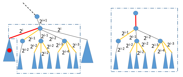
Figure 7: Example where major edge is not the parent of the relevant subtree. The major edge is in red, the key edges in yellow, and the red circle is the location of the algorithm’s server. In this situation, the server is in $T_{e}$ as shown and $X_{e}=R_{e}$. The dotted boxes show the edges in the critical subtree $C_{e}$. In particular, the figure on the right shows the transformation of the critical subtree, where the major edge is now depicted as the parent of the relevant subtree.

The ps algorithm only serves requests in the relevant subtree $R_{e}$ of the major edge $e$ that triggered the serving phase. Recall from the introduction that the algorithm performs two kinds of service: critical service and preemptive service. First, we partition unserved requests in $R_{e}$ into two groups.

Unserved requests in the relevant subtree $R_{e}$ that are connected to the major edge $e$ by saturated edges are said to be critical, while other unserved requests in $R_{e}$ are said to be non-critical.

The algorithm serves all critical requests in $R_{e}$ in the serving phase. This is called critical service. In addition, it also serves a subset of non-critical requests in $R_{e}$ as preemptive service. Next, we describe the selection of non-critical requests for preemptive service.

Preemptive Service. We would like to piggyback the cost of preemptive service on critical service. Let us call the subtree connecting the major edge $e$ to the critical requests in $R_{e}$ the critical subtree $C_{e}$ (we also include $e$ in $C_{e}$). Recall that $e$ may either be a sibling or the parent of the top layer of edges in $R_{e}$ (Fig. 8). Even in the first case, in $C_{e}$, we make $e$ the parent of the top layer of edges in $R_{e}$ for technical reasons (see Fig. 7 for an example of this transformation). Note that this does not violate the HST property of $C_{e}$ since the length of $e$ is at least $2$ times that of any other edge in $R_{e}$, by virtue of $e$ being the major edge for all requests in $R_{e}$.

The cost of critical service is the total length of edges in the critical subtree $C_{e}$. However, using this as the cost bound for preemptive service in the ps algorithm causes some technical difficulties. Rather, we identify a subset of edges (we call these key edges) in $C_{e}$ whose total length is at least $1/h$ times that of all edges in $C_{e}$. We define key edges next.

Let us call two edges related if they form an ancestor-descendant pair in $C_{e}$ . A cut in $C_{e}$ is a subset of edges, no two of which are related, and whose removal disconnects all the leaves of $C_{e}$ from its root.

The set of key edges is formed by the cut of maximum total edge length in the critical subtree $C_{e}$. If there are multiple such cuts, any one of them is chosen arbitrarily.

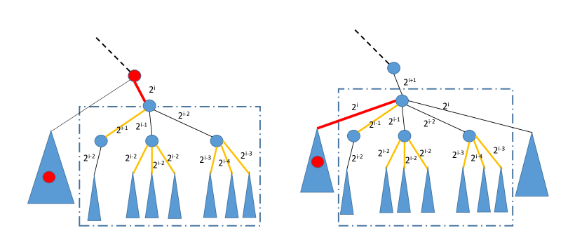
Figure 8: The two possible configurations of the major edge (in red) vis-à-vis the relevant subtree. The subtree surrounded by dashed box is the relevant subtree. The red nodes are possible locations of the server. The edges in yellow are key edges. In the figure to the right, note that the edge of length $2^{i}$ to the right is not included in the relevant subtree.

The reader is referred to Fig. 8 for an example of key edges. Note that either the major edge $e$ is the unique key edge, or the key edges are a set of total length at least $\ell(e)$ whose removal disconnects $e$ from all critical requests in the relevant subtree $R_{e}$. It is not difficult to see that the total length of the key edges is at least $1/h$ times that of all edges in $C_{e}$.

We will perform recursive time forwarding on the key edges to identify the requests for preemptive service. Consider any single key edge $e$. Let us denote the subtree below $e$ in the HST by $T_{e}$. Typically, when we are forwarding time on a key edge $e$, we consider requests in subtree $T_{e}$. However, there is one exception: if $e$ is the major edge and is a sibling of the top layer of its relevant subtree (Fig. 8), then we must consider requests in the relevant subtree $R_{e}$. We define a single notation for both cases:

For any key edge $e$, let $X_{e}$ denote the following:

• If the algorithm’s server is not in $T_{e}$, then $X_{e}=T_{e}$.

• If the algorithm’s server is in $T_{e}$, then $X_{e}=R_{e}$.

To serve critical requests, the server must traverse a key edge $e$ and enter $X_{e}$. Now, suppose $X_{e}$ looks exactly like Fig. 1, i.e., there is a single critical request and many non-critical requests. As we saw in the introduction, the server cannot afford to only serve the critical request, but must also do preemptive service. Our basic principle in doing preemptive service is to simulate future time and serve requests in $X_{e}$ that would become critical the earliest. So, we forward time into the future, which causes the critical subtree in $X_{e}$ to grow. But, our total budget for preemptive service in $X_{e}$ is only $\ell(e)$, the length of $e$. (This is because the overall budget for preemptive service in this serving phase is the sum of lengths of all the key edges. This budget is distributed by giving a budget equal to its length to each key edge.) This budget cap implies that we should stop time forwarding once the critical subtree in $X_{e}$ has total edge length $\ell(e)$; otherwise, we will not have enough budget to serve the requests that have become critical after time forwarding. As was the case earlier, working with the entire critical subtree in $X_{e}$ is technically difficult. Instead, we forward time until there is a cut in the critical subtree of $X_{e}$ whose total edge length is equal to $\ell(e)$ (at this point, we say edge $e$ is over-saturated). This cut now forms the next layer of edges in the recursion (we call these service edges). Note that the key edges form the first layer of service edges in the recursion. Extending notation, $X_{e^{\prime}}=T_{e^{\prime}}$ for all service edges in subsequent layers of recursion. We recursively forward time on each of these service edges $e^{\prime}$ in their respective subtrees $X_{e^{\prime}}$ using the same process.

How does the recursion stop? Note that if the current service edge $e^{\prime}$ is a leaf edge, then the recursion needs to stop since the only vertex in $X_{e^{\prime}}$ is already critical at the time the previous recursive level forwarded to. More generally, if all requests in $X_{e^{\prime}}$ become critical without any cut in the critical subtree of $X_{e^{\prime}}$ attaining total length $\ell(e^{\prime})$, then we are assured that the cost of serving all requests in $X_{e^{\prime}}$ is at most $h$ times the cost of traversing edge $e^{\prime}$. In this case, we do not need to forward time further on $e^{\prime}$ (indeed, time forwarding does not change the critical subtree since all requests are already critical), and the recursion ends.

We now give a formal description of this recursive time forwarding process. For any edge $e$, let ${\tt child}(e)$ be the edges in the first layer of subtree $X_{e}$. (When $X_{e}=T_{e}$, these are simply the children edges of $e$. But, in the special case where $X_{e}=R_{e}$, these are the siblings of $e$ of smaller length than $e$.) We define

$$f(e)=\begin{cases}\max\left(\ell(e),\sum_{e_{i}\in{\tt child}(e)}{f(e_{i})}\right)&\text{if }e\text{ is saturated.}\\ 0&\text{otherwise.}\end{cases}$$

This allows us to formally define over-saturation, that we intuitively described above.

An edge $e$ is said to be over-saturated if either of the following happens:

• $e$ is saturated and $\sum_{e_{i}\in{\tt child}(e)}{f(e_{i})}\geq\ell(e)$, i.e., $f(e)$ is determined by $\sum_{e_{i}\in{\tt child}(e)}{f(e_{i})}$ in the formula above (we call this over-saturation by children).

• All requests in $X_{e}$ are connected to $e$ via saturated edges.

Using this notion of over-saturation, the ps algorithm now identifies a set of edges $S$ that the server will traverse in the relevant subtree $R_{e}$ of the major edge $e$ that triggered the serving phase. In the formal description, we will not consider critical service separately since the edges in the critical subtree $C_{e}$ will be the first ones to be added to $S$ in our recursive Time-Forwarding process. Initially, all saturated edges between the key edges and the major edge, both inclusive, are added to $S$. This ensures that the algorithm traverses each key edge. Now, the algorithm performs the following recursive process on every key edge $e^{\prime}$ in subtree $X_{e}$.

Intuitively, the edges in $G(e)$ are the ones that form the maximum length cut in the critical subtree of $X_{e}$ at time $t$ (we show this property formally in Lemma 9). In the recursive step, ideally we would like to recurse on all edges in $G(e)$. However, if $e_{l}$ is the last edge added to $G(e)$ during Time-Forwarding($e$), it is possible that $\sum_{e^{\prime}\in G(e)\setminus\{e_{l}\}}\ell(e^{\prime})<f(e)$ but $\sum_{e^{\prime}\in G(e)}\ell(e^{\prime})>f(e)$. In this case, we cannot afford to recurse on all edges in $G(e)$ since their total length is greater than that of $e$. This is why we select the subset $H(e)$ whose sum of edge lengths is exactly equal to that of $e$. We show in Lemma 6 below that this is always possible to do. The set of edges that we call Time-Forwarding on, i.e., the key edges and the union of all $H(e)$’s in the recursive algorithm, are called service edges.

Lemma 6.

Let $e$ be an edge oversaturated by children. $G(e)$ represents a set of saturated but not over-saturated edges satisfying:

$$\sum_{e^{\prime}\in G(e)}\ell(e^{\prime})=\sum_{e^{\prime}\in G(e)}f(e^{\prime})\geq\ell(e).$$

Then, there is some subset $H(e)\subseteq G(e)$ such that $\sum_{e^{\prime}\in H(e)}\ell(e^{\prime})=\ell(e)$.

Proof.

Note that all edge lengths are of the form $2^{i}$ for non-negative integers $i$. Furthermore, the length of every edge in $G(e)$ is strictly smaller than the length of $e$. Thus, the lemma is equivalent to showing that for any set of elements of the form $2^{i}$ (for some $i\leq j-1$) that sum to at least $2^{j}$, there exists a subset of these elements that sum to exactly $2^{j}$.

First, note that we can assume that the sum of these elements is strictly smaller than $(3/2)\cdot 2^{j}$. If not, we repeatedly discard an arbitrarily selected element from the set until this condition is met. Since the discarded value is at most $2^{j-1}$ at each stage, the sum cannot decrease from $\geq(3/2)\cdot 2^{j}$ to $<2^{j}$ in one step.

Now, we use induction on the value of $j$. For $j=1$, the set can only contain elements of value $2^{0}=1$, and sums to the range $[1,3)$. Clearly, the only option is that there are two elements, both of value $1$. For the inductive step, order the elements in decreasing value. There are three cases:

• If there are $2$ elements of value $2^{j-1}$, we output these $2$ elements.

• If there is $1$ element of value $2^{j-1}$, we add it to our output set. Then, we start discarding elements in arbitrary order until the remaining set has total value less than $(3/2)\cdot 2^{j-1}$. Then, we apply the inductive hypothesis on the remaining elements.

• Finally, suppose there is no element of value $2^{j-1}$ in the set. We greedily create a subset by adding elements to the subset in arbitrary order until their sum is at least $2^{j-1}$. Since each element is of value at most $2^{j-2}$, the total value of this subset is less than $(3/2)\cdot 2^{j-1}$. Call this set A. Now, we are left with elements summing to total value at least $2^{j-1}$ and less than $2^{j}$. We again repeat this process to obtain another set $B$ of total value in the range $[2^{j-1},(3/2)\cdot 2^{j-1})$. We now recurse on these two subsets $A$ and $B$.∎

Once all chains of recursion have ended, the server does a DFS on the edges in $S$, serving all requests it encounters in doing so. After this, the server stops at the bottom of the last key edge visited.

Remark: If the HST is an embedding of a general metric space, then the leaves in the HST are the only actual locations on the metric space. So, when the ps algorithm places the server at an intermediate vertex, the server is actually sent to a leaf in the subtree under that vertex in the actual metric space. It is easy to see that this only causes a constant overhead in the service cost. Note that this does not affect the ps algorithm’s operation at all; it operates as if the server were at the non-leaf vertex.

Finally, the algorithm resets the counters, i.e., sets $w(e)=0$, for all edges $e$ that it traverses in the serving phase.

This completes the description of the algorithm.

3 Competitive Ratio of Preemptive Service Algorithm

In this section, we show that the ps algorithm described in the previous section has a competitive ratio of $O(h^{3})$ on an HST of depth $h$ (Theorem 2), which implies a competitive ratio of $O(\log^{4}n)$ on general metric spaces (Theorem 1).

First, we specify the location of requests that can put weight on an edge at any time in the ps algorithm.

Lemma 7.

At any time, for any edge $e$, the weight on edge $e$ is only due to unserved requests in $X_{e}$.

Proof.

When the server serves a request, it traverses all edges on its path to the request and resets their respective counters. So, the only possibility of violating the lemma is due to a change in the definition of $X_{e}$. But, for the definition of $X_{e}$ to change, the server must traverse edge $e$ and reset its counter. This completes the proof. ∎

Next, we observe that the total delay penalty of the algorithm is bounded by its service cost. (Recall that the service cost is the distance moved by the server.)

Lemma 8.

The total delay penalty is bounded by the total service cost.

Proof.

By design of the algorithm, every unserved request always increases the counter on some edge with its instantaneous delay penalty. The lemma now follows from the observation that the counter on an edge $e$ can be reset from at most $\ell(e)$ to $0$ only when the server moves on the edge incurring service cost $\ell(e)$. ∎

Next, we show that the total service cost can be bounded against the length of the key edges. First, we formally establish some properties of the Time-Forwarding process that we intuitively stated earlier.

Lemma 9.

When the algorithm performs Time-Forwarding($e$), then the following hold:

• If a saturated edge $e^{\prime}\in X_{e}$ is not over-saturated by its children, all cuts in the saturated subtree in $X_{e^{\prime}}$ have total edge length at most $\ell(e^{\prime})$.

• $\sum_{e^{\prime}\in G(e)}\ell(e^{\prime})\leq(3/2)\ell(e)$.

• $G(e)$ is the cut of maximum total edge length in the saturated subtree of $X_{e}$ at time $t$, the time when $e$ is first over-saturated.

Proof.

The first property follows from the fact that for a saturated edge $e^{\prime}$, the definition of the function $f(.)$ implies that the value of $f(e^{\prime})$ is at least the sum of lengths of any cut in the saturated subtree of $X_{e^{\prime}}$ at time $t$.

For the second property, note that every edge in $X_{e}$ has length at most $\ell(e)/2$, and use Lemma 6.

Now, suppose the third property is violated, and there is a larger saturated cut $G^{\prime}(e)$. Since $G(e)$ over-saturates all its ancestor edges, it follows that for any such ancestor edge $\tilde{e}$ in $X_{e}$, the descendants of $\tilde{e}$ in $G(e)$ have total length at least $\ell(\tilde{e})$. Thus, there must be an edge $e^{*}\in G(e)$ such that the sum of lengths of the descendants of $e^{*}$ in $G^{\prime}(e)$ is greater than $\ell(e^{*})$. But, if this were the case, $e^{*}$ would be over-saturated, which contradicts the definition of $G(e)$. ∎

Lemma 10.

The total service cost is at most $O(h^{2})$ times the sum of lengths of key edges.

Proof.

By the HST property, the distance traveled by the server from its initial location to the major edge $e$ is at most $O(1)$ times $\ell(e)$. But, $\ell(e)$ is at most the total length of the key edges, since $e$ itself is a valid cut in the critical subtree $C_{e}$. Hence, we only consider server movement in the relevant subtree $R_{e}$.

Now, consider the edges connecting the major edge to the key edges. Let the key edges have total length $L$. Consider the cut comprising the parents of all the key edges. They also form a valid cut, and hence, their total length is at most $L$. We repeat this argument until we get to the major edge. Then, we have at most $h$ cuts, each of total edge length at most $L$. Thus the total length of all edges connecting the major edge to the key edges is at most $h$ times the length of the key edges.

This brings us to the edges traversed by the server in the subtrees $X_{e}$, for key edges $e$. We want to bound their total length by $O(h^{2}\cdot\ell(e))$. We will show a more general property: that for any service edge $e$, the total length of edges traversed in $X_{e}$ is $O(h^{2}\cdot\ell(e))$. First, we consider the case that the recursion ends at $e$, i.e., $e$ was not over-saturated by its children. By Lemma 9, this implies that every cut in the saturated subtree in $X_{e}$ has total length at most $\ell(e)$. In particular, we can apply this to the layered cuts (children of the key edges, their children, and so on) in the saturated subtree. There are at most $h$ such cuts covering the entire saturated subtree, implying that the total cost of traversing the saturated edges in $X_{e}$ is $O(h\cdot\ell(e))$.

Next, we consider the case when $e$ is over-saturated by its children. We use an inductive argument on the height of the subtree $X_{e}$. Suppose this height is $h$. Further, let the edges in $H(e)$ (that we recurse on in Time-Forwarding($e$)) be $e_{1},e_{2},\ldots$, where the height of subtree $X_{e_{i}}$ is $h_{i}\leq h-1$. By definition of $H(e)$, we have $\sum_{i}\ell(e_{i})=\ell(e)$. Using the inductive hypothesis, the total cost inside subtree $X_{e_{i}}$ is at most $C\cdot h_{i}^{2}\cdot\ell(e_{i})$ for some constant $C$. Summing over $i$, and using $h_{i}\leq h-1$, we get that the total cost is at most $C\cdot(h-1)^{2}\cdot\ell(e)$. This leaves us with the cost of reaching the critical requests in $X(e^{\prime})$ for each $e^{\prime}\in G(e)$, from edge $e$. We can partition these edges into at most $h$ layers, where by Lemma 9, the total cost of each such layer is at most $(3/2)\cdot\ell(e)$. It follows that the total cost of all layers is at most $(3/2)\cdot h\cdot\ell(e)$. Adding this to the inductive cost, the total cost is at most $C\cdot h^{2}\cdot\ell(e)$ for a large enough $C$. This completes the inductive proof. ∎

Now, we charge the lengths of all key edges to the optimal solution opt. Most of the key edges will be charged directly to opt, but we need to define a potential function $\Phi$ for one special case. For a fixed optimal solution, we define $\Phi$ as

$$\Phi=\kappa d(\mbox{alg's server},\mbox{{\tt opt}'s server}).$$

In words, $\Phi$ is equal to $\kappa$ times the distance between algorithm’s server and opt’s server. Here, $\kappa=ch^{2}$ for a large enough constant $c$. Overall, we use a charging argument to bound all costs and potential changes in our algorithm to opt such that the charging ratio is $O(h^{3})$.

The first case is when the major edge $e$ is the only key edge, and opt’s server is in $X_{e}$. Then, all costs are balanced by the decrease in potential.

Lemma 11.

When the major edge $e$ is the only key edge, and opt’s server is in $X_{e}$, the sum of change in potential function $\Phi$ and the service cost is non-positive.

Proof.

This is immediate from the definition of $\Phi$ and Lemma 10. ∎

In other cases, we charge all costs and potential changes to either opt’s waiting cost or opt’s moving cost by using what we call a charging tree.

A charging tree is a tree of (service edge, time interval) pairs. For each service edge $e$ at time $t$, let $t^{\prime}$ be the last time that $e$ was a service edge ($t^{\prime}=0$ if $e$ was never a service edge in the past). Then, $(e,[t^{\prime},t))$ is a node in a charging tree. We simultaneously define a set of charging trees, the roots of which exactly correspond to nodes $(e,[t^{\prime},t))$ where $e$ is a key edge at time $t$.

To define the charging trees, we will specify the children of a node $(e,[t^{\prime},t))$:

• The node $(e,[t^{\prime},t))$ is a leaf in the charging tree if $t^{\prime}=0$ or $e$ is not over-saturated by children at time $t^{\prime}$ (i.e., all previously unserved requests in $X_{e}$ were served at time $t^{\prime}$).

• Otherwise, let $H(e)$ be as defined in Time-Forwarding($e$). For any $e^{\prime}\in H(e)$, let $t^{\prime\prime}$ be the last time that $e^{\prime}$ was a service edge. Then, for each $e^{\prime}\in H(e)$, $(e^{\prime},[t^{\prime\prime},t^{\prime}))$ is a child of $(e,[t^{\prime},t))$.

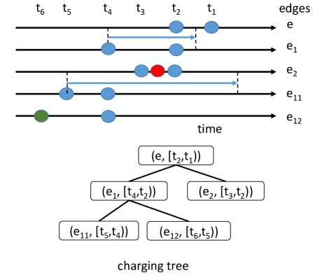
Figure 9: Example of a charging tree. On the top is the timeline corresponding to the charging tree on the bottom. The blue circles represent that the corresponding edge is a service edge in the serving phase of the algorithm at that time. The red circle indicates that opt’s server traverses the edge in the interval defined the two blue circles surrounding the red circle. The green circle indicates that the corresponding edge is not only a service edge in the serving phase of the algorithm at that time, but that the algorithm actually served all requests in the corresponding subtree $X_{e_{12}}$.

See Fig. 9 for an example. This figure shows a charging tree with 5 nodes: $(e,[t_{2},t_{1}))$, $(e_{1},[t_{4},t_{2}))$, $(e_{2},[t_{3},t_{2}))$, $(e_{11},[t_{5},t_{4}))$, $(e_{12},[t_{6},t_{4}))$.

We say that opt incurs moving cost at a charging tree node $(e,[t^{\prime},t))$ if it traverses edge $e$ in the time interval $[t^{\prime},t)$. Next, we incorporate opt’s delay penalties in the charging tree. We say that opt incurs waiting cost of $\ell(e)$ at a charging tree node $(e,[t^{\prime},t))$, if there exists some (future) time $t^{*}\geq t$ such that:

• opt’s server is never in $X_{e}$ in the time interval $[t^{\prime},t^{*})$, and

• the requests that arrive in $X_{e}$ in the time interval $[t^{\prime},t)$ have a total delay penalty of at least $\ell(e)$ if they remain unserved at time $t^{*}$.

Intuitively, if these conditions are met, then opt has a delay penalty of at least $\ell(e)$ from only the requests in subtree $T_{e}$ that arrived in the time interval $[t^{\prime},t)$.

Without loss of generality, we assume that at time 0, opt traverses all the edges along the paths between the starting location of the server and all requests. (Since these edges need to be traversed at least once by any solution, this only incurs an additive cost in opt, and does not change the competitive ratio by more than a constant factor.)

Now, we prove the main property of charging trees.

Lemma 12 (Main Lemma).

For any key edge $e$ served at time $t$ by the algorithm, if opt’s server was not in $X_{e}$ at time $t$, then opt’s waiting and moving cost in the charging tree rooted at $(e,[t^{\prime},t))$ is at least $\ell(e)$.

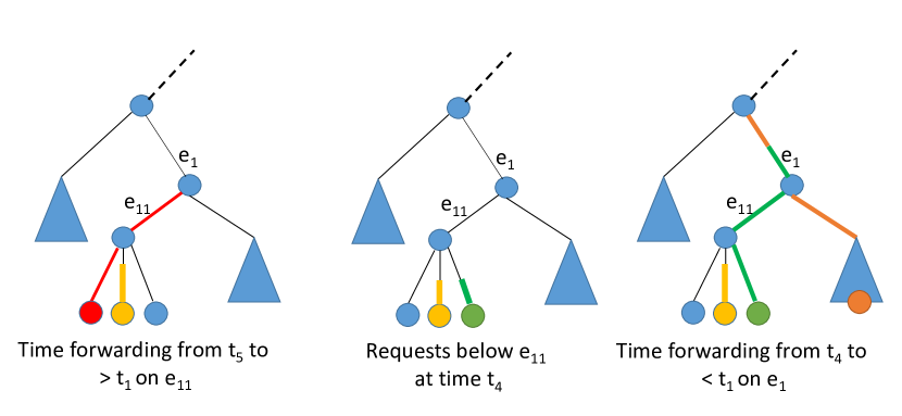
Figure 10: Illustration of Case 2 in Lemma 12. The left figure shows the time forwarding for $e_{11}$ at time $t_{5}$. All the red requests are served at $t_{5}$. The center figure shows the waiting time below $e_{11}$ at time $t_{4}$. Note that since $t_{4}<t$, the yellow requests could not reach $e_{11}$, and the green requests are requests that came between $t_{5}$ and $t_{4}$. The right figure shows the time forwarding process for $e_{1}$ at time $t_{4}$. We know $e_{11}$ must be saturated because it is a child in charging tree. However, the yellow requests cannot contribute to $e_{11}$ because they do not even reach $e_{11}$ at time $t$. Therefore, all the weight on $e_{11}$ must come from green requests.

Proof.

We use the recursive structure of the charging tree. Suppose the root of the tree is $(e,[t^{\prime},t))$, the current node we are considering is $(u,[t_{u}^{\prime},t_{u}))$, and the parent of the current node is $(v,[t_{v}^{\prime},t_{v}))$. (Here, $u$ and $v$ are edges in the HST.) By the structure of the charging tree, we know that $t_{v}^{\prime}=t_{u}$. We will now list a set of conditions. At node $(u,[t_{u}^{\prime},t_{u}))$, if one of these conditions holds, then we show that the waiting or moving cost incurred by opt at this node is at least $\ell(u)$, the length of edge $u$. Otherwise, we recurse on all children of this charging tree node. The recursion will end with one these conditions being met.

Case 1. opt crossed edge $u$ in the time interval $[t_{u}^{\prime},t_{u})$: This is the case for $(e_{2},[t_{3},t_{2}))$ in Fig. 9. In this case, opt incurs moving cost of $\ell(u)$ at node $(u,[t_{u}^{\prime},t_{u}))$ of the charging tree.

Case 2. Case 1 does not apply, and the algorithm forwarded time to greater than $t$ in Time-Forwarding($u$) at time $t_{u}^{\prime}$: This is the case for $(e_{11},[t_{5},t_{4}))$ in Fig. 9. A detailed illustration of this case is given in Fig. 10. Note that Case 1 does not apply to $(u,[t_{u}^{\prime},t_{u}))$ by definition. Moreover, Case 1 also does not apply to any of the ancestors of this node in the charging tree; otherwise, the recursive charging scheme would not have considered the $(u,[t_{u}^{\prime},t_{u}))$ node. Furthermore, at time $t$, opt’s server was not in $X_{e}$ by the condition of the lemma. These facts, put together, imply that opt could not have served any request in $X_{u}$ in the time interval $[t_{u}^{\prime},t)$ . In particular, this implies that opt could not have served requests in $X_{u}$ that arrived in the time interval $[t_{u}^{\prime},t_{u})$ before time $t$(these are green requests in Fig. 10).

We now need to show that these requests have a total delay penalty of at least $\ell(u)$ by time $t$. Since Time-Forwarding($u$) forwarded time beyond $t$ at time $t_{u}^{\prime}$, any request in $X_{u}$ that arrived before $t_{u}^{\prime}$ and put weight on edge $u$ (these are red requests in Fig. 10) must have been served at time $t_{u}^{\prime}$. The requests left unserved (yellow requests in Fig. 10) do not put weight on edge $u$ even after forwarding time to $t$.

Now, note that no ancestor of the $(u,[t_{u}^{\prime},t_{u}))$ node in the charging tree can be in Case 2, else the recursive charging scheme would not consider the $(u,[t_{u}^{\prime},t_{u}))$ node. Therefore, Time-Forwarding($v$) must have forwarded time to at most $t$ at time $t_{v}^{\prime}=t_{u}$. Suppose we reorder requests so that the requests that arrived earlier put weight first (closer to the request location), followed by requests that arrived later. Then, the requests in $X_{u}$ that arrived before $t_{u}^{\prime}$ but were not served at time $t_{u}^{\prime}$ (yellow requests in Fig. 10) do not put weight on edge $u$ in Time-Forwarding($v$) at time $t_{v}^{\prime}$, since time is being forwarded to less than $t$. Therefore, the only requests in $X_{u}$ that put weight on edge $u$ in Time-Forwarding($v$) at time $t_{v}^{\prime}$ arrived in the time interval $[t_{u}^{\prime},t_{u})$ (green requests in Fig. 10). By Lemma 7, at any time, the only requests responsible for the weight on edge $u$ are requests in $X_{u}$. Therefore, the requests that arrived in $X_{u}$ in the time interval $[t_{u}^{\prime},t_{u})$ saturate edge $e$ in Time-Forwarding($v$) at time $t_{v}^{\prime}$. In other words, these requests incur delay penalties of at least $\ell(u)$ if they are not served till time $t$. Since opt did not serve any of these requests before time $t$, it follows that opt incurs waiting cost of $\ell(u)$ at node $(u,[t)u^{\prime},t_{u}))$ of the charging tree.

Case 3. Case 1 does not apply, and all requests in $X_{u}$ were served by the algorithm at time $t_{u}^{\prime}$: This is the case for $(e_{12},[t_{6},t_{4}))$ in Fig. 9. Similar to the previous case, Time-Forwarding($v$) at time $t_{v}^{\prime}$ must have been to at most time $t$. Since all requests in $X_{u}$ that arrived before time $t_{u}^{\prime}$ were served at time $t_{u}^{\prime}$, the requests that saturated edge $u$ in Time-Forwarding($v$) at time $t_{v}^{\prime}=t_{u}$ must have arrived in the time interval $[t_{u}^{\prime},t_{u})$ (same argument as in Case 2). As in Case 2, opt could not have served these requests before time $t$, and hence incurs delay penalty of at least $\ell(u)$ on these requests. Therefore, opt incurs waiting cost of $\ell(u)$ at node $(u,[t_{u}^{\prime},t_{u}))$ of the charging tree.

By the construction of charging tree, the leaves are either in Case 3, or has starting time $0$ (which is in Case 1). So, this recursive argument always terminates.

Note that each key edge is the root of a charging tree, and for each node of the charging tree, the length of the corresponding edge is equal to the sum of lengths of the edges corresponding to its children nodes. Therefore when the argument terminates, we can charge the cost of the key edge to a set of nodes in the charging tree whose total cost is exactly equal to the cost of the key edge. ∎

So, we have shown that the length of key edges can be bounded against opt’s cost on the charging tree. But, it is possible that in this analysis, we are using the same cost incurred by opt in multiple charging tree nodes. In other words, we need to bound the cost incurred by opt at charging tree nodes against the actual cost of opt.

Lemma 13.

The total number of charging tree nodes on which the same request causes opt to incur cost is at most $h+1$.

Proof.

First, note that the charging tree nodes corresponding to the same edge $e$ represent disjoint time intervals. This implies that for a given request that arrived at time $t$, opt only incurs cost in the charging tree node $(e,[t_{1},t_{2}))$ where $t\in[t_{1},t_{2})$. We now show that the total number of different edges for which the same request is counted toward opt’s cost at charging tree nodes is at most $h+1$.

To obtain this bound, we observe that there are two kinds of edges we need to count: (1) edges on the path from the request to the root of the HST, and (2) edges for which the request is in the relevant subtree. Clearly, there are at most $h$ category (1) edges. But, there can be a much larger number of category (2) edges. However, we claim that among these category (2) edges, opt incurs cost in the charging tree at a node corresponding to at most one edge. To see this, we observe the following properties:

• If opt incurs cost at a charging tree node corresponding to a category (2) edge $e$, then opt’s server must be in $T_{e}$ at the arrival time of the request.

• The category (2) edges are unrelated in the HST, i.e., for any two such edges $e_{1},e_{2}$, we have the property that $T_{e_{1}}$ and $T_{e_{2}}$ are disjoint.∎

Finally, we are ready to prove the main theorem (Theorem 2).

Proof of Theorem 2.

Recall that we bound both the delay penalties and service cost of the algorithm by the total length of key edges times $O(h^{2})$, in Lemmas 8 and 10. Now, we will charge the total length of key edges to $O(h)$ times opt’s costs. Consider a serving phase at time $t$.

Case (a). Suppose opt’s server is not in subtree $X_{e}$ of a key edge $e$. Then, by Lemma 12, opt incurs a cost of at least $\ell(e)$ in the charging tree rooted at $(e,[t^{\prime},t))$, where $t^{\prime}$ is the last time when $e$ was a service edge. On the other hand, opt’s moving cost can be counted by at most one node in all charging trees, and by Lemma 13, opt’s waiting cost can be counted by at most $h+1$ nodes in all charging trees. Therefore the total length of Case (a) key edges is bounded by $(h+1)$ times the cost of opt.

Case (b). Now, let us consider the situation where opt’s server is in the subtree $X_{e}$ for a key edge $e$. There are two possibilities:

• Case (b)(i). If $e$ is also the major edge, it must be the unique key edge and we apply Lemma 11.

• Case (b)(ii). Otherwise, $e$ is not the major edge. Then, any single key edge can be of length at most half the major edge, but the key edges add up to at least the length of the major edge. Thus, any single key edge only accounts for at most half the total length of key edges. Now, opt’s server can be in the subtree $T_{e}$ for only one of the key edges $e$ (note that in this case, $T_{e}=X_{e}$ since the major edge is not the unique key edge). It follows that the key edges in Case (a) account for at least half the total length of the key edges. In this case, we can charge the Case (b) key edges to the Case (a) key edges (which are, in turn, charged to opt by the argument above).

Finally, we also need to bound the change in potential during this serving phase in Case (a) and Case (b)(ii). Note that if $e$ is the major edge, the server’s final location is at a distance of at most $4\ell(e)$ from the server’s initial solution (the server first reaches the major edge, then crosses the major edge, and eventually ends on the other side of some key edge). Therefore, the total change in potential is at most $4\kappa\ell(e)$, which is also bounded by $O(h^{2})$ times the total length of the key edges. ∎

4 Online Service with Delay: $k$ Servers

We now generalize the osd problem to $k$ servers, for any $k\geq 1$. We call this the $k$-osd problem. Again, we only give an algorithm for the $k$-osd problem on HSTs, which yields an algorithm for the $k$-osd problem on general metric spaces by a low-distortion tree embedding [33]. But, before stating this result, let us first note that the $k$-osd problem generalizes the well-studied $k$-server problem [46, 28, 27, 44, 43, 17, 13]. This latter problem is exactly identical to the $k$-osd problem, except that every request must be served immediately on arrival (consequently, there is no delay and therefore, no delay penalty). But, this can be modeled in the osd problem by using an infinite delay penalty for every request. Furthermore, this also establishes a connection between $k$-osd and paging problems [49, 34, 47, 51, 1, 37, 14], as will be discussed in Section 5.1 and 5.2.

We now re-state our results for $k$-osd (Theorem 4 in the introduction).

Theorem 14.

There is a deterministic algorithm with a competitive ratio of $O(kh^{4})$ for the $k$-osd problem on an HST of depth $h$. As immediate corollaries, this yields the following:

• A randomized algorithm with a competitive ratio of $O(k\log^{5}n)$ for the $k$-osd problem on general metric spaces.

• A deterministic algorithm with a competitive ratio of $O(k)$ for the unweighted and weighted paging problems with delay penalties, which are respectively special cases of $k$-osd on the uniform metric and star metrics.

We will discuss the paging problems in Section 5.1 and Section 5.2. In this section, we will focus on proving Theorem 4 on HSTs.

To generalize our algorithm for osd from a single server to $k$ servers, we use ideas from the so-called active cover algorithm for $k$-server on trees by Chrobak and Larmore [28]. This algorithm is a generalization of the well-known double cover algorithm [27] for $k$-server on the line metric.

In the active server algorithm, we define active servers as the ones that are directly connected to the request location on the tree, i.e., there is no other server on the path connecting the request to an active server. To serve a request, the algorithm moves all active servers simultaneously at the same speed to the request, until one of these servers reaches the request and serves it.

4.1 Algorithm

We use the intuition of moving all active servers toward a request in our $k$-osd algorithm as well. To describe the algorithm, we specify how we modify the waiting phase and serving phase of the algorithm.

Waiting Phase. During the waiting phase, for each server, the algorithm has a separate counter on each edge and increments this counter exactly as in the osd algorithm assuming this is the only server. The waiting phase ends when for any of these servers, a major edge is saturated. (Note that set of major edges may be different for different servers, since it depends on the location of the server.)

Remark: In our $k$-osd algorithm, we allow a server to reside in the middle of an edge during a waiting phase. If this is the case, and if for any request, the segment of the edge on which the server is residing is longer than all the other edges on the path between the server and the request, then we call this segment the major edge. Also, note that we do not need to actually place a server at the middle of an edge in an implementation; instead, we can simply delay moving the server until it reaches the other end of the edge. The abstraction of placing a server on an edge, however, will make it easier to visualize our algorithm, and to do the analysis.

Serving Phase. We apply the same Time-Forwarding subroutine from the ps algorithm for the osd problem to determine the key edges, as well as the edges that will be traversed in the relevant subtree. Now, the algorithm needs to decide which server to use in this service. This is decided in two phases. First, we order the key edges in a DFS order, with the property that siblings are ordered in non-decreasing length. We then assume that every key edge has a request at its end, and use the active cover algorithm to serve these (imaginary) requests. Initially, the active cover algorithm moves all active servers toward the first key edge, and the unique server that reaches it first actually crosses this key edge. We now need to serve an actual set of requests in the subtree below this key edge. To serve these requests, the server that traversed the key edge performs a DFS tour and returns to the base of the key edge. Note that we are not using the active cover algorithm during this service, i.e., all other servers do not move. Once this server returns to the base of the key edge, the active cover algorithm again resumes toward the next key edge in our pre-determined order. Once all requests that were selected to be served have indeed been served, the server that was serving requests below the last key edge returns to the base of this key edge.

4.2 Analysis

To analyze the new algorithm, we need to use the same potential function as the active cover algorithm [28]. Define potential function $\Phi$ to be

$$\Phi=\kappa(k||M_{\min}||+\sum_{i<j}||s_{i}s_{j}||).$$

Here, $M_{\min}$ is the minimum-cost matching (mcm) between the algorithm’s servers and opt’s servers for a fixed optimal solution opt. $||M_{\min}||$ denotes the cost of the matching, i.e., the sum of lengths of edges in $M_{\min}$. In the potential function, $s_{1},\ldots,s_{k}$ denote the locations of the algorithm’s servers. We choose then parameter $\kappa$ to be $Ch^{2}$ for a large enough constant $C$ (note that this is similar to what we did for the ps algorithm with $k=1$).

We first summarize the properties of this potential function. (The subtree below a node $v$, including $v$ itself, is denoted by $T_{v}$.)

Lemma 15.

The first property concerns opt’s movement:

• When opt moves a server by distance $d$, the potential function can increase by at most $\kappa kd$.

Now, suppose the algorithm moves all active servers at equal speed toward a node $v$ in the tree. Further, suppose the algorithm does not have any server in the subtree $T_{v}$. Then, we have:

• If opt has a server in $T_{v}$, then the potential function decreases by $\kappa$ times the total distance traveled by the algorithm’s servers.

• If opt does not have a server in $T_{v}$, then the potential function can increase by at most $2k\kappa$ times the movement of any one of algorithm’s servers.

Proof.

We prove each property separately:

• By the triangle inequality, the cost of the previous mcm increases by at most $d$, and the cost of this matching is an upper bound on the cost of the new mcm.

• Suppose each of algorithm’s servers travels distance $d$. Furthermore, let the number of active servers be $q$, where the $i$th active server resides on the path connecting $r_{i}$ servers to $v$. Then, the distance between the $i$th active server and $r_{i}$ servers increases by $d$, its distance to the remaining $(k-r_{i}-q)$ inactive servers decreases by $d$, and its distance to the remaining $q-1$ active servers decreases by $2d$. Overall, the change in the second term in $\Phi$ is given by:

  $$d\cdot\kappa\cdot\sum_{i=1}^{q}(2r_{i}-k+1)=d\cdot\kappa\cdot\left[2(k-q)-kq+q\right]$$

  $$=d\cdot\kappa\cdot\left[2k-q-kq\right]$$

  The change in the first term is only due to the $q$ active servers, of which one can wlog be matched with opt’s server in $T_{v}$. Therefore, the change in the first term is at most:

  $$d\cdot\kappa\cdot\left[kq-2k\right].$$

  Adding these two expressions shows that the decrease of potential is at least $\kappa\cdot(qd)$.

• We again get the same expression as above for the change in the second term of $\Phi$. For the first term, the change is at most

  $$d\cdot\kappa\cdot kq.$$

  Adding these two expressions, the potential increases by at most

  $$\kappa\cdot(2kd-qd)\leq\kappa\cdot(2kd).\qed$$

Using these properties, we are now going to establish that our $k$-osd algorithm is $O(kh^{3})$-competitive (Theorem 4). We follow a similar strategy as our osd algorithm — we will again show the moving cost and waiting cost can all be charged to the cost of the key edges (we will lose an extra factor of $k$ here). There are several new issues that now arise that are specific to $k$ being more than $1$. But first, we show that service inside the subtrees $X_{e}$ for key edges $e$ is analogous to the single server scenario. (Recall the definition of $X_{e}$ from Section 2.)

Lemma 16.

When the serving phase begins, none of the algorithm’s servers is in the relevant subtree.

Proof.

Suppose not: there is a server $s$ in the relevant subtree. Let $s^{\prime}$ be the server whose major edge was saturated first. We will call edges saturated/unsaturated according to the state of their counters for $s^{\prime}$. Consider the path between $s$ and the end of the major edge that is not in the relevant subtree $R_{e}$ (let us call this vertex $v$). (If the major edge is only part of an edge, then this path also ends at the same location in the middle of the edge. Indeed, throughout this lemma, we will treat the major edge as a full edge, although it may really only be a segment of an edge.) Traversing this path from $v$, let $e$ be the first edge that is unsaturated, and $e^{\prime}$ be the saturated edge immediately before $e$ on this path. Note that $e^{\prime}$ must exist because the major edge is saturated.

The length of edge $e$ is at most the length of $e^{\prime}$ because either $e^{\prime}$ is the parent of $e$ in the HST or $e^{\prime}$ is the major edge. Let $u$ be the vertex shared by $e$ and $e^{\prime}$. If there is a saturated edge $e^{\prime\prime}$ in the subtree $T_{u}$ that has length at least the length of $e$, then $e^{\prime\prime}$ is a saturated major edge for $s$. Otherwise, since edge $e^{\prime}$ is saturated for $s^{\prime}$, and all the requests in $X_{e^{\prime}}$ will contribute to edge $e$ for server $s$, edge $e$ would be saturated before $e^{\prime}$. Therefore, there cannot be a server in the relevant subtree. ∎

Note that Lemma 8 still holds for $k$-osd. Therefore, we can charge all delay penalties to service costs of the algorithm up to a constant factor.

Lemma 17.

The total delay penalties incurred by the $k$-osd algorithm is at most the total service cost of the algorithm.

The service costs come in two parts. The first part is the cost of traversing edges inside the subtrees $X_{e}$ for key edges $e$. Lemma 10 still holds as well; therefore, the service cost inside subtrees $X_{e}$ for key edges $e$ is at most $O(h^{2})$ times the sum of lengths of key edges.

Lemma 18.

The total service cost inside the subtree $X_{e}$ for a key edge $e$ is at most $O(h^{2})$ times $\ell(e)$, the length of $e$.

Now, we need to analyze the service cost of traversing the subtree connecting the major edge and the key edges, including both the major edge and the key edges. These are the parts where the active cover algorithm is being used.

First, we state a general property analogous to Lemma 11, that bounds the change in potential when the servers move.

Lemma 19.

At any time in the active cover algorithm, if all of the algorithm’s servers are moving toward some server in opt, then the potential decreases by $\kappa$ times the distance moved by the servers.

Proof.

This follows directly from Lemma 15. ∎

Furthermore, let us consider a subtree $X_{e}$ for a key edge $e$, where $X_{e}$ does not contain any of opt’s servers. In this case, we use the same charging tree argument as in the ps algorithm. Note that since Lemma 7 still holds. So, we can apply Lemmas 12 and 13 to bound the lengths of the key edges against opt’s costs up to a factor of $O(h)$.

Lemma 20.

The sum of lengths of all key edges $e$ such that the subtrees $X_{e}$ does not contain any of opt’s servers is at most $O(h)$ times the cost of opt.

Proof.

This follows directly from Lemmas 12 and 13. ∎

First, note that if the major edge is the solitary key edge, then Lemmas 18, 19, and 20 are sufficient to bound the total service cost by $O(kh^{3})$ times the cost of opt. Therefore, in the rest of this section, we will assume that the key edges are distinct from the major edge.

For a saturated edge $e$ that is between the major edge and key edges (including the major edge and key edges themselves), we call the subtree $X_{e}$ a charging branch if:

• opt does not have a server in $X_{e}$, and

• $e$ is the major edge, or opt has a server in the subtree $X_{p(e)}$ for the parent $p(e)$ of $e$ in the critical tree $C_{e}$.

In this case, we call $e$ the root edge of the charging branch.

Note that every key edge $e$ such that opt does not have a server in $X_{e}$ belongs to one of the charging branches. Conversely, any charging branch contains one or more such key edges. The total service cost of the algorithm in a charging branch is defined as the algorithm’s cost between serving the last key edge outside charging branch, and serving the last key edge inside the charging branch.

Lemma 21.

The sum of algorithm’s service cost in serving requests in a charging branch and the change in potential is at most $O(kh^{3})$ times the sum of lengths of key edges in the charging branch.

Proof.

Let $e$ be the root edge of the charging branch. The service cost of the algorithm in the charging branch can be divided into three parts:

1. the service cost incurred between serving the last request outside the charging branch till a server reaches edge $e$,

2. the service cost of using the active cover algorithm between the key edges in $S$, and

3. the cost of preemptive service below the key edges.

Let $\ell$ be the sum of lengths of key edges in the charging branch.

Lemma 18 implies that the service cost of (3) is at most $O(h^{2}\ell)$. Next, observe that by the definition of key edges, the service cost of (2) for any single server is at most $O(h\ell)$, and therefore, at most $O(kh\ell)$ counting all the servers. Furthermore, by Lemma 15, the increase in potential due to (2) (note that (3) does not change potential) is at most $2k\kappa$ times the service cost of any single server, the latter being at most $O(h\ell)$. Therefore, the total service cost and increase in potential due to (2) and (3) is at most $O(kh^{3}\ell)$.

Now we deal with cost of (1). If $e$ is the major edge, then the distance traversed by any single server to the major edge is $O(1)$ times the length of the major edge, which is $O(\ell)$ since the sum of lengths of key edges is at least the length of the major edge. The corresponding change in potential is $O(kh^{2}\ell)$.

Now, suppose $e$ is not the major edge. In this case, note that $p(e)$, the parent edge of $e$, must be in the critical tree $C_{e}$ and that OPT is in $X_{p(e)}$. Then, there are two cases:

• First, consider the situation that the algorithm has not served any request in the current serving phase before reaching edge $e$. In this case, algorithm’s servers are moving toward one of opt’s servers until one of them traverses $e$. By Lemma 19, the decrease in potential is sufficient to account for the service cost of the algorithm in (1).

• Next, consider the situation that the algorithm did serve requests in the current serving phase before reaching edge $e$. Let $e^{\prime}$ be the last key edge for which the algorithm served requests in $X_{e^{\prime}}$. There are two subcases:

  • Suppose $p(e)$, the parent edge of $e$ in the critical subtree $C_{e}$, is not an ancestor of $e^{\prime}$. Then, we know that the algorithm does not have a server in $X_{p(e)}$ by Lemma 16 and the fact that no request in $X_{p(e)}$ has been served yet. In this case, we again have the property that algorithm’s servers are moving toward one of opt’s servers until one of them traverses $e$. By Lemma 19, the decrease in potential is sufficient to account for the service cost of the algorithm in (1).

  • Now, suppose $p(e)$ is an ancestor of $e^{\prime}$ as well. Recall that in the DFS order used by the algorithm between key edges, siblings are ordered in non-decreasing length. This implies that the distance from $e^{\prime}$ to $e$ is at most $2$ times the length of $e$. As a consequence, the total distance traversed by a single server in (1) is at most $2$ times the length of $e$. Therefore, we can charge the service cost in (1) to $O(\ell)$ and the potential increase in (1) to $O(kh^{2}\ell)$.∎

We are now ready to bound the total cost of the algorithm against the cost of opt.

Lemma 22.

The total service and delay cost in the $k$-osd algorithm is $O(kh^{4})$ times the cost of opt.

Proof.

First, we bound the total service cost. We partition the total movement of any single server into phases: we say that that the algorithm is in phase $e$ for a key edge $e$ is the active cover algorithm is moving the active servers toward the imaginary request at the end of edge $e$, or a server is serving requests in $X_{e}$.

Phases are of two kinds:

• If opt has a server in $X_{e}$, then the sum of potential change and service costs in phase $e$ is non-positive by Lemma 19.

• We are left with the phases where opt does not have a server in $X_{e}$ for phase $e$. These phases are partitioned into super-phases defined by the charging branch that $e$ belongs to - that is, for each charging phase we define a super-phase, and then include phase $e$ in the super-phase of the charging branch $e$ belongs to. For each such super-phase, by Lemma 21, the total service cost and potential change is at most $O(kh^{3})$ times the length of the key edges in the charging branch, $\ell$. Furthermore, by Lemma 20, $\ell$ can be bounded by $O(h)$ times the cost of ${\tt opt}$.

Since the potential function is non-negative, it follows that the total service cost of the $k$-osd algorithm is at most $O(kh^{4})$ times the cost of opt,

Finally, by Lemma 17, we bound the total delay penalties of the algorithm to be at most the total service cost. This completes the proof. ∎

This shows that the competitive ratio of the $k$-osd algorithm is $O(kh^{4})$.

5 Special Metrics

In this section, we present algorithms for the $k$-osd problem on special metric spaces: uniform and star metrics. These respectively correspond to the paging and weighted paging problems with delay.

5.1 Uniform Metric/Paging

We give a reduction from the $k$-osd problem on a uniform metric to the classical online paging problem. The reduction is online, non-clairvoyant, and preserves the competitive ratio up to a constant. To describe this reduction, it would be convenient to view the $k$-osd problem on a uniform metric as the following equivalent problem that we call paging with delay:

There are $n$ pages that issue requests over time. Each request is served when the corresponding page is brought into a cache that can only hold $k<n$ pages at a time. The algorithm can bring a page into the cache and evict an existing page, this process being called a page swap and having a cost of one. For every request, the algorithm also incurs a delay penalty, which is a monotone function of the delay in serving the request. The algorithm can only access the current value of the delay penalty.

Classical paging is the special case of this problem when every request has an infinite delay penalty, i.e., each request must be served immediately, and the total cost is the number of page swaps.

Suppose we are given an instance $\mathcal{I}$ of the paging problem with delay. We will reduce it to an instance $\mathcal{I^{\prime}}$ of classical online paging. The requests for a page $p$ in $\mathcal{I}$ are partitioned into time intervals such that the total delay penalty incurred by the requests in an interval is exactly one at the end of the interval. In instance $\mathcal{I^{\prime}}$, this interval is now replaced by a single request for $p$ at the end of the interval. (See Fig. 11(a).) Note that the reduction is online and non-clairvoyant. We now show that by this reduction, any algorithm for $\mathcal{I^{\prime}}$ can be used for $\mathcal{I}$, losing only a constant in the competitive ratio.

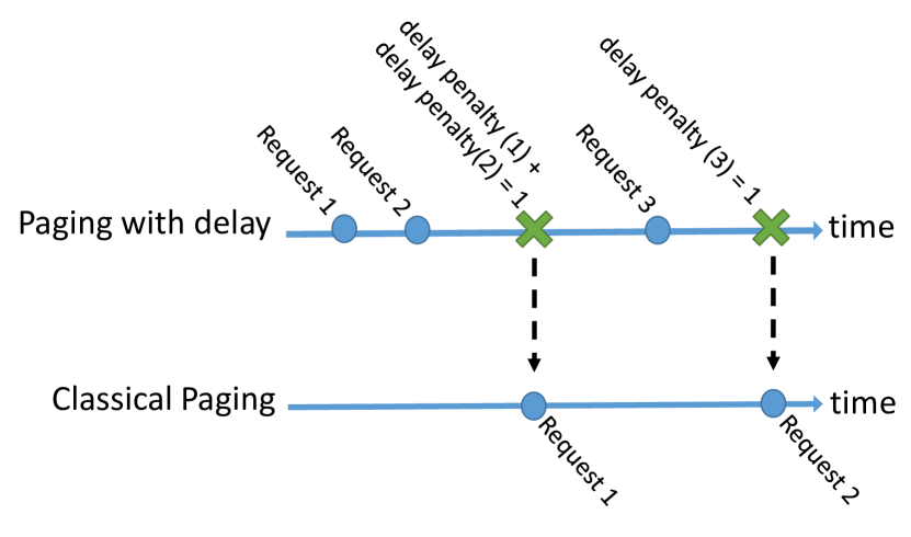
(a) The reduction between instances for unweighted paging. This figure shows the requests for a single page.

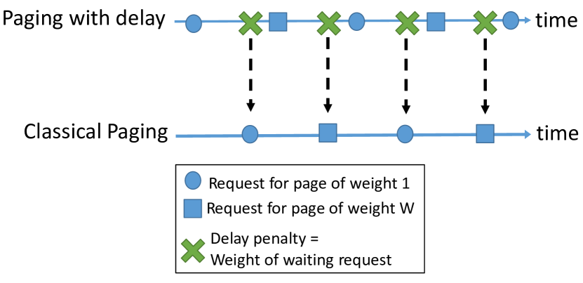
(b) An example where the reduction has a large gap for weighted paging.

Figure 11: The reduction between instances of online paging with delay and classical online paging: it works for unweighted paging, but fails for weighted paging.

Lemma 23.

The optimal cost in $\mathcal{I}^{\prime}$ is at most 3 times the optimal cost in $\mathcal{I}$. Conversely, the cost of an algorithm in $\mathcal{I}$ is at most 2 times that in $\mathcal{I}^{\prime}$.

Proof.

Let us denote the optimal costs in $\mathcal{I}$ and $\mathcal{I}^{\prime}$ by ${\tt opt}_{\mathcal{I}}$ and ${\tt opt}_{\mathcal{I}^{\prime}}$ respectively. Similarly, let ${\tt alg}_{\mathcal{I}}$ and ${\tt alg}_{\mathcal{I}^{\prime}}$ respectively denote the cost of an algorithm in $\mathcal{I}$ and $\mathcal{I}^{\prime}$.

Construct a solution for $\mathcal{I}^{\prime}$ that maintains exactly the same cache contents as the optimal solution for $\mathcal{I}$ at all times. Whenever there is a request for a page that is not in the cache, it serves the page and then immediately restores the cache contents of ${\tt opt}_{\mathcal{I}}$ by performing the reverse swap and restoring the previous page in the cache. Note that there are two types of page swaps being performed: the first category are those that are also performed by ${\tt opt}_{\mathcal{I}}$, and the second category are the pairs of swaps to serve requests for pages not in the cache. The total number of page swaps in the first category is identical the number of page swaps in ${\tt opt}_{\mathcal{I}}$. For the second category, if a page $p$ is not in the cache at the end of an interval in $\mathcal{I}$, there are two possibilities. If no request for $p$ in the preceding interval was served in ${\tt opt}_{\mathcal{I}}$ during the interval, then the total delay penalty for these requests at the end of the interval is 1. On the other hand, if some request for $p$ in the preceding interval was served in ${\tt opt}_{\mathcal{I}}$ during the interval, but the page is no longer in the cache at the end of the interval, then there was at least 1 page swap that removed $p$ from the cache during the interval. In either case, we can charge the two swaps performed in $\mathcal{I}^{\prime}$ to the cost of 1 that ${\tt opt}_{\mathcal{I}}$ incurs in this interval for page $p$.

In the converse direction, note that by definition, the swap cost of ${\tt alg}_{\mathcal{I}}$ is identical to that of ${\tt alg}_{\mathcal{I}^{\prime}}$. The only difference is that in $\mathcal{I}$, the algorithm also suffers a delay penalty. The delay penalty for a page in an interval is 0 if the algorithm maintains the page in the cache throughout the interval, and at most 1 otherwise. In the latter case, the algorithm must have swapped the page out during the interval since the page was in the cache at the end of the previous interval. In this case, we can charge the delay penalty in ${\tt alg}_{\mathcal{I}}$ to this page swap during the interval that ${\tt alg}_{\mathcal{I}^{\prime}}$ incurred. ∎

Using the above lemma and the well-known and asymptotically tight $O(k)$-competitive deterministic and $O(\log k)$-competitive randomized algorithms for online paging (see, e.g., [20]), we obtain the following theorem.

Theorem 24.

There are $O(k)$-competitive deterministic and $O(\log k)$-competitive randomized algorithms for online paging with delay (equivalently, $k$-osd on the uniform metric). This implies, in particular, that there is an $O(1)$-competitive deterministic algorithm for osd on uniform metrics. These results also apply to the non-clairvoyant version of the problems, where the delay penalties in the future are unknown to the algorithm. These competitive ratios are asymptotically tight.

5.2 Star Metric/Weighted Paging

As in the case of the uniform metric, it will be convenient to view the $k$-osd problem on a star metric as a paging problem with delay, the only difference being that every page $p$ now has a non-negative weight $w_{p}$ which is the cost of evicting the page from the cache. Note that in this case the aspect ratio $\Delta$ of the star metric is (up to a constant factor) the ratio of the maximum and minimum page weights.

For weighted paging, suppose we try to use the reduction strategy for (unweighted) paging from the previous section. We can now partition requests for a page $p$ into intervals, where the total delay penalty at the end of the interval is the weight of the page $w_{p}$. This reduction, however, fails even for simple instances. Consider two pages of weights $W$ and $1$, where $W\gg 1$. Suppose their requests have penalty equal to their respective weights for unit delay. If the requests for the pages alternate, and the cache can only hold only a single page, the algorithm repeatedly swaps the pages, whereas an optimal solution keeps the heavy page in the cache and serves the light page only once every $W$ time units. The gap induced by the reduction in this instance is $W$. (See Fig. 11(b).)

Indeed, we show that this difficulty is fundamental in that there is no good non-clairvoyant algorithm for the weighted paging problem with delay.

Theorem 25.

There is a lower bound of $\Omega(W)$ on the competitive ratio of weighted paging with delay, even with a single-page cache (equivalently, osd on a star metric) in the non-clairvoyant setting, where $W$ is the ratio of the maximum to minimum page weight (equivalently, aspect ratio $\Delta$ of the star metric).

Proof.

Suppose there is a heavy page $p_{0}$ with cost $W$ (without loss of generality assume $W$ is an integer), and all other pages $p_{1},p_{2},...,p_{n}$ have cost $1$. Set $n=W^{2}$. We will construct an adversarial instance based on how the algorithm decides to serve the pages. The instance is constructed in phases: at the beginning of each phase, there is a request for all of the small pages $p_{1},...,p_{n}$. However, the waiting cost for all of these requests start at $0$, and at some time $t$ (not necessarily in the same phase) will become infinity; we say that this request becomes critical at time $t$. The adversary will control the time that requests become critical. For each phase, we maintain the following properties:

1. At the beginning of each phase, all the small pages have a request.

2. The algorithm either serves all the small pages at least once, or serves page $p_{0}$ at least $W$ times, in each phase.

3. The optimal solution does not incur any waiting cost. In each phase, the optimal solution serves $p_{0}$ once and at most $W$ of the small pages.

Given these properties, it is easy to check that the competitive ratio of the algorithm is at least $W/2$, because in each phase algorithm spends at least $W^{2}$, while the optimal spends at most $2W$.

Now we describe how the adversary works. At time $\epsilon$ (for any fixed $\epsilon$ strictly between $0$ and $1$), there is a request for $p_{0}$ that requires immediate service. At time $t=1,2,...,W$, if the algorithm has not served all the small pages at least once in this phase, let $r_{t}\in\{1,2,...,n\}$ denote the index of an unserved page. The adversary makes $p_{r_{t}}$ critical at time $t$, and adds a request for $p_{0}$ at time $t+\epsilon$. Note that page $p_{0}$ must be in the algorithm’s cache at time $t-1+\epsilon$ and at time $t+\epsilon$, but cannot be in the algorithm’s cache at time $t$. Thus, the algorithm must evict $p_{0}$ at least once in this interval. Therefore, at the end of time $W+1$, either the algorithm has served all the small pages at least once in this phase, or it has served $p_{0}$ at least $W$ times.

The optimal solution serves $p_{r_{1}}$, $p_{r_{2}}$, $\dots$, $p_{r_{t}}$ at time $0$, and $p_{0}$ at time $\epsilon$. Since no other page became critical in this phase, the optimal solution will never need to evict $p_{0}$ in this phase.

After time $W+1$, the adversary generates a request for each of the small pages, and starts a new phase. If this procedure repeats for $k$ phases, then the algorithm’s cost is at least $kW^{2}$, while the optimal solution’s cost is at most $2kW+n$ (the optimal solution serves all non-critical requests at the very end). Therefore, as $k$ goes to infinity, the competitive ratio of the algorithm cannot be better than $W/2$. ∎

The above theorem implies that we must restrict ourselves to the clairvoyant setting for the weighted paging with delay problem. For this case, our results for osd/$k$-osd on a star metric follow as corollaries of our theorems for general metrics (Theorems 2, 4).

Theorem 26.

There is an $O(k)$-competitive deterministic algorithm for online weighted paging with delay (equivalently, $k$-osd on a star metric). This implies, in particular, an $O(1)$-competitive deterministic algorithm for the osd problem on star metrics. These competitive ratios are asymptotically tight for deterministic algorithms.

References

- [1] Dimitris Achlioptas, Marek Chrobak, and John Noga. Competitive analysis of randomized paging algorithms. Theor. Comput. Sci., 234(1-2):203–218, 2000.
- [2] Anna Adamaszek, Artur Czumaj, Matthias Englert, and Harald Räcke. Almost tight bounds for reordering buffer management. In STOC, pages 607–616, 2011.
- [3] Esther M Arkin, Joseph SB Mitchell, and Giri Narasimhan. Resource-constrained geometric network optimization. In SOCG, pages 307–316. ACM, 1998.
- [4] Giorgio Ausiello, Esteban Feuerstein, Stefano Leonardi, Leen Stougie, and Maurizio Talamo. Competitive algorithms for the on-line traveling salesman. In Algorithms and Data Structures, 4th International Workshop, WADS ’95, Kingston, Ontario, Canada, August 16-18, 1995, Proceedings, pages 206–217, 1995.
- [5] Giorgio Ausiello, Esteban Feuerstein, Stefano Leonardi, Leen Stougie, and Maurizio Talamo. Algorithms for the on-line travelling salesman. Algorithmica, 29(4):560–581, 2001.
- [6] Noa Avigdor-Elgrabli, Sungjin Im, Benjamin Moseley, and Yuval Rabani. On the randomized competitive ratio of reordering buffer management with non-uniform costs. In Automata, Languages, and Programming - 42nd International Colloquium, ICALP 2015, Kyoto, Japan, July 6-10, 2015, Proceedings, Part I, pages 78–90, 2015.
- [7] Noa Avigdor-Elgrabli and Yuval Rabani. An improved competitive algorithm for reordering buffer management. In SODA, pages 13–21, 2010.
- [8] Noa Avigdor-Elgrabli and Yuval Rabani. An optimal randomized online algorithm for reordering buffer management. CoRR, abs/1303.3386, 2013.
- [9] Baruch Awerbuch, Yossi Azar, Avrim Blum, and Santosh Vempala. New approximation guarantees for minimum-weight k-trees and prize-collecting salesmen. SIAM Journal on Computing, 28(1):254–262, 1998.
- [10] Yossi Azar, Ashish Chiplunkar, and Haim Kaplan. Polylogarithmic bounds on the competitiveness of min-cost perfect matching with delays. In Proceedings of the Twenty-eighth Annual ACM-SIAM Symposium on Discrete Algorithms, SODA 2017, Barecelona, Spain, 2017.
- [11] Yossi Azar and Adi Vardi. TSP with time windows and service time. CoRR, abs/1501.06158, 2015.
- [12] Nikhil Bansal, Avrim Blum, Shuchi Chawla, and Adam Meyerson. Approximation algorithms for deadline-tsp and vehicle routing with time-windows. In STOC, pages 166–174. ACM, 2004.
- [13] Nikhil Bansal, Niv Buchbinder, Aleksander Madry, and Joseph Naor. A polylogarithmic-competitive algorithm for the k-server problem. J. ACM, 62(5):40, 2015.
- [14] Nikhil Bansal, Niv Buchbinder, and Joseph Naor. A primal-dual randomized algorithm for weighted paging. J. ACM, 59(4):19, 2012.
- [15] Reuven Bar-Yehuda, Guy Even, and Shimon Moni Shahar. On approximating a geometric prize-collecting traveling salesman problem with time windows. Journal of Algorithms, 55(1):76–92, 2005.
- [16] Siddharth Barman, Shuchi Chawla, and Seeun Umboh. A bicriteria approximation for the reordering buffer problem. In ESA, pages 157–168, 2012.
- [17] Yair Bartal and Elias Koutsoupias. On the competitive ratio of the work function algorithm for the k-server problem. Theor. Comput. Sci., 324(2-3):337–345, 2004.
- [18] Marcin Bienkowski, Martin Böhm, Jaroslaw Byrka, Marek Chrobak, Christoph Dürr, Lukáš Folwarczný, Lukasz Jez, Jiri Sgall, Nguyen Kim Thang, and Pavel Veselý. Online algorithms for multi-level aggregation. In 24th Annual European Symposium on Algorithms, ESA 2016, August 22-24, 2016, Aarhus, Denmark, pages 12:1–12:17, 2016.
- [19] Avrim Blum, Shuchi Chawla, David R Karger, Terran Lane, Adam Meyerson, and Maria Minkoff. Approximation algorithms for orienteering and discounted-reward tsp. In Foundations of Computer Science, 2003. Proceedings. 44th Annual IEEE Symposium on, pages 46–55. IEEE, 2003.
- [20] Allan Borodin and Ran El-Yaniv. Online Computation and Competitive Analysis. Cambridge University Press, New York, NY, USA, 1998.
- [21] Niv Buchbinder, Moran Feldman, Joseph (Seffi) Naor, and Ohad Talmon. O(depth)-competitive algorithm for online multi-level aggregation. In Proceedings of the Twenty-Eighth Annual ACM-SIAM Symposium on Discrete Algorithms, SODA 2017, Barcelona, Spain, Hotel Porta Fira, January 16-19, pages 1235–1244, 2017.
- [22] Niv Buchbinder, Kamal Jain, and Joseph Naor. Online primal-dual algorithms for maximizing ad-auctions revenue. In Algorithms - ESA 2007, 15th Annual European Symposium, Eilat, Israel, October 8-10, 2007, Proceedings, pages 253–264, 2007.
- [23] Niv Buchbinder, Tracy Kimbrel, Retsef Levi, Konstantin Makarychev, and Maxim Sviridenko. Online make-to-order joint replenishment model: Primal-dual competitive algorithms. Operations Research, 61(4):1014–1029, 2013.
- [24] Chandra Chekuri and Nitish Korula. Approximation algorithms for orienteering with time windows. arXiv preprint arXiv:0711.4825, 2007.
- [25] Chandra Chekuri, Nitish Korula, and Martin Pál. Improved algorithms for orienteering and related problems. ACM Transactions on Algorithms (TALG), 8(3):23, 2012.
- [26] Chandra Chekuri and Amit Kumar. Maximum coverage problem with group budget constraints and applications. In Approximation, Randomization, and Combinatorial Optimization. Algorithms and Techniques, pages 72–83. Springer, 2004.
- [27] Marek Chrobak, H Karloof, T Payne, and S Vishwnathan. New ressults on server problems. SIAM Journal on Discrete Mathematics, 4(2):172–181, 1991.
- [28] Marek Chrobak and Lawrence L Larmore. An optimal on-line algorithm for k servers on trees. SIAM Journal on Computing, 20(1):144–148, 1991.
- [29] Daniel R. Dooly, Sally A. Goldman, and Stephen D. Scott. On-line analysis of the TCP acknowledgment delay problem. J. ACM, 48(2):243–273, 2001.
- [30] Yuval Emek, Shay Kutten, and Roger Wattenhofer. Online matching: haste makes waste! In Proceedings of the 48th Annual ACM SIGACT Symposium on Theory of Computing, STOC 2016, Cambridge, MA, USA, pages 333–344, 2016.
- [31] Matthias Englert, Harald Räcke, and Matthias Westermann. Reordering buffers for general metric spaces. Theory of Computing, 6(1):27–46, 2010.
- [32] Matthias Englert and Matthias Westermann. Reordering buffer management for non-uniform cost models. In ICALP, pages 627–638, 2005.
- [33] Jittat Fakcharoenphol, Satish Rao, and Kunal Talwar. A tight bound on approximating arbitrary metrics by tree metrics. J. Comput. Syst. Sci., 69(3):485–497, 2004.
- [34] Amos Fiat, Richard M. Karp, Michael Luby, Lyle A. McGeoch, Daniel Dominic Sleator, and Neal E. Young. Competitive paging algorithms. J. Algorithms, 12(4):685–699, 1991.
- [35] Iftah Gamzu and Danny Segev. Improved online algorithms for the sorting buffer problem on line metrics. ACM Transactions on Algorithms, 6(1):15:1–15:14, 2009.
- [36] Bruce L Golden, Larry Levy, and Rakesh Vohra. The orienteering problem. Naval research logistics, 34(3):307–318, 1987.
- [37] Sandy Irani. Randomized weighted caching with two page weights. Algorithmica, 32(4):624–640, 2002.
- [38] Sandy Irani, Xiangwen Lu, and Amelia Regan. On-line algorithms for the dynamic traveling repair problem. Journal of Scheduling, 7(3):243–258, 2004.
- [39] Anna R. Karlin, Claire Kenyon, and Dana Randall. Dynamic TCP acknowledgment and other stories about e/(e-1). Algorithmica, 36(3):209–224, 2003.
- [40] Yoshiyuki Karuno and Hiroshi Nagamochi. 2-approximation algorithms for the multi-vehicle scheduling problem on a path with release and handling times. Discrete Applied Mathematics, 129(2):433–447, 2003.
- [41] Rohit Khandekar and Vinayaka Pandit. Online sorting buffers on line. In STACS, pages 584–595, 2006.
- [42] Sanjeev Khanna, Joseph Naor, and Danny Raz. Control message aggregation in group communication protocols. In Automata, Languages and Programming, 29th International Colloquium, ICALP 2002, Malaga, Spain, July 8-13, 2002, Proceedings, pages 135–146, 2002.
- [43] Elias Koutsoupias. Weak adversaries for the k-server problem. In 40th Annual Symposium on Foundations of Computer Science, FOCS ’99, 17-18 October, 1999, New York, NY, USA, pages 444–449, 1999.
- [44] Elias Koutsoupias and Christos H. Papadimitriou. On the k-server conjecture. J. ACM, 42(5):971–983, 1995.
- [45] Sven O Krumke, Nicole Megow, and Tjark Vredeveld. How to whack moles. In Approximation and Online Algorithms, pages 192–205. Springer, 2004.
- [46] Mark S. Manasse, Lyle A. McGeoch, and Daniel Dominic Sleator. Competitive algorithms for server problems. J. Algorithms, 11(2):208–230, 1990.
- [47] Lyle A. McGeoch and Daniel Dominic Sleator. A strongly competitive randomized paging algorithm. Algorithmica, 6(6):816–825, 1991.
- [48] Harald Räcke, Christian Sohler, and Matthias Westermann. Online scheduling for sorting buffers. In ESA, pages 820–832, 2002.
- [49] Daniel Dominic Sleator and Robert Endre Tarjan. Amortized efficiency of list update and paging rules. Commun. ACM, 28(2):202–208, 1985.
- [50] John N Tsitsiklis. Special cases of traveling salesman and repairman problems with time windows. Networks, 22(3):263–282, 1992.
- [51] Neal E. Young. The k-server dual and loose competitiveness for paging. Algorithmica, 11(6):525–541, 1994.