Nonnegative Restricted Boltzmann Machines for Parts-based Representations Discovery and
Predictive Model Stabilization

Abstract

The success of any machine learning system depends critically on effective representations of data. In many cases, it is desirable that a representation scheme uncovers the parts-based, additive nature of the data. Of current representation learning schemes, restricted Boltzmann machines (RBMs) have proved to be highly effective in unsupervised settings. However, when it comes to parts-based discovery, RBMs do not usually produce satisfactory results. We enhance such capacity of RBMs by introducing nonnegativity into the model weights, resulting in a variant called nonnegative restricted Boltzmann machine (NRBM). The NRBM produces not only controllable decomposition of data into interpretable parts but also offers a way to estimate the intrinsic nonlinear dimensionality of data, and helps to stabilize linear predictive models. We demonstrate the capacity of our model on applications such as handwritten digit recognition, face recognition, document classification and patient readmission prognosis. The decomposition quality on images is comparable with or better than what produced by the nonnegative matrix factorization (NMF), and the thematic features uncovered from text are qualitatively interpretable in a similar manner to that of the latent Dirichlet allocation (LDA). The stability performance of feature selection on medical data is better than RBM and competitive with NMF. The learned features, when used for classification, are more discriminative than those discovered by both NMF and LDA and comparable with those by RBM.

1 Introduction

Learning meaningful representations from data is often critical to achieve high performance in machine learning tasks bengio_etal_pami13_representation . An attractive approach is to estimate representations that best explain the data without the need for labels. One important class of such methods is the restricted Boltzmann machine (RBM) smolensky_mit86_information ; freund_haussler_techrep94_unsupervised , an undirected probabilistic bipartite model in which a representational hidden layer is connected with a visible data layer. The weights associated with connections encode the strength of influence between hidden and visible units. Each unit in the hidden layer acts as a binary feature detector, and together, all the hidden units are linearly combined through the connection weights to form a fully distributed representation of data hinton_ghahramani_biosci97_generative ; bengio_etal_pami13_representation . This distributed representation is highly compact: for $\mathrm{K}$ units, there are $2^{\mathrm{K}}-1$ non-empty configurations that can explain the data.

However, the fully distributed representation learned by RBMs may not interpretably disentangle the factors of variation since the learned features are often global, that is, all the data units must play the role in one particular feature. As a result, learned features do not generally represent parts and components teh_etal_nips01_rbmrate . For example, the facial features learned by RBM depicted in Fig. 1a are generally global; it is hard to explain how a face is constructed from these parts. Parts-based representations, on the other hand, are perceptually intuitive. Using the same facial example, if individual parts of the face (e.g. eyes, nose, mouth, forehead as in Fig. 1c) are discovered, it would be easy to construct the face from these parts. In terms of modeling, detecting parts-based representation also improves the object recognition performance agarwal_etal_pami04_learning .

One of the best known techniques to achieve parts-based representation is nonnegative matrix factorization (NMF) lee_etal_nature99_nmf . In NMF, the data matrix is approximately factorized into a basis matrix and a coding matrix, where all the matrices are assumed to be nonnegative. Each column of the basis matrix is a learned feature, which could be sparse under appropriate regularization hoyer_jmlr04_nmf . The NMF, however, has a fundamental drawback: it does not generalize to unseen data since there is no mechanism by which a new data point can be generated from the learned model. Instead, new representations must be learned from the expensive “fold-in” procedure. The RBM, on the other hand, is a proper generative model – once the model has been learned, new samples can be drawn from the model distribution. Moreover, due to the special bipartite structure, estimating representation from data is efficient with a single matrix operation.

In this paper, we derive a novel method based on the RBM to discover useful parts whilst retaining its discriminative capacity. As inspired by the NMF, we propose to enforce nonnegativity in the connection weight matrix of the RBM. Our method integrates a barrier function into the objective function so that the learning is skewed towards nonnegative weights. As the contribution of the visible units towards a hidden unit is additive, there exists competition among visible units to activate the hidden unit leading to a small portion of connections surviving. In the same facial example, the method could achieve parts-based representation of faces, which is, surprisingly, even better than what learned by the standard NMF (cf. Fig. 1). We term the resulting model the nonnegative restricted Boltzmann machine (NRBM).

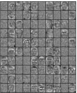
(a) RBM

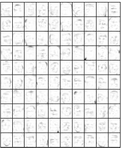
(b) NMF

(c) NRBM

Figure 1: Representations learned from the ORL face image database att_orl using the ordinary RBM, NMF and NRBM on the left, middle, right, respectively. Darker pixels show larger weights.

In addition to parts-based representation, there are several benefits with this nonnegativity constraint. First, in many cases, it is often easier to make sense of addition of new latent factors (due to nonnegative weights) than of subtraction (due to negative weights). For instance, clinicians may be more comfortable with the notion that a risk factor either contributes positively to a disease development or not at all (e.g., the connections have zeros weights). Second, as weights can be either positive or zero, the parameter space is highly constrained leading to potential robustness. This can be helpful when there are many more hidden units than those required to represent all factors of variation: extra hidden units will automatically be declared “dead” if all connections to them cannot compete against others in explaining the data. Lastly, combining two previous advantages, the NRBM effectively gathers related important features, e.g., key risk factors that explain the disease, into groups at the data layer and encourages less hidden units to be useful at hidden layer. This helps to stabilize linear predictive models by providing hidden representations for them to perform on.

We demonstrate the effectiveness of the proposed model through comprehensive evaluation on three real-world applications using five real datasets of very different natures.

• The first application is parts-based discovery. Our primary targets are to decompose images into interpretable parts (and receptive fields), e.g., dots and strokes in handwritten digits (MNIST dataset lecun_etal_mnist ), and facial components in faces (CBCL mit_cbcl and ORL att_orl databases); and to discover plausible latent thematic features, which are groups of semantically related words (TDT2 text corpus cai_etal_tkde05_document ).

• The second application is feature extraction for classification. Here we apply our models on MNIST, TDT2 and heart failure datasets. The learned features are then fed into standard classifiers. The experiments reveal that the classification performance is comparable with the standard RBM, and competitive against NMF (on all images, text, and medical records) and latent Dirichlet allocation (on text) blei_etal_jmlr03_lda .

• The last one is linear classifier stabilization. The goal is to enhance feature and model stabilities in clinical prognosis. The experimental results on heart failure patients show significant improvements of stability scores over linear sparse model and the RBM, and better prediction performances than those of RBM and NMF. This application in healthcare analytics is the main extension of our previous model introduced in tu_etal_acml13_nrbm .

In short, our main contributions are: (i) the derivation of the nonnegative restricted Boltzmann machine, a probabilistic machinery that has the capacity of learning parts-based representations; (ii) a comprehensive evaluation the capability of our method as a representational learning tool on image, text and medical data, both qualitatively and quantitatively; and (iii) a demonstration of stabilizing linear classifiers in clinical prognosis.

The rest of the paper is structured as follows. Section 3 presents the derivation and properties of our nonnegative RBM, followed by its applications in linear predictive model stabilization in Section 4. We then report our experimental results in Section 5. Section 6 provides a discussion of the related literature. Finally, Section 7 concludes the paper.

2 Preliminaries

We first describe the restricted Boltzmann machine (RBM) for unsupervised learning representation. An RBM smolensky_mit86_information ; freund_haussler_techrep94_unsupervised ; hinton_neucom02_cd is a bipartite undirected graphical model in which the bottom layer contains observed variables called visible units and the top layer consists of latent representational variables, known as hidden units. Two layers are fully connected but there is no connection within layers. The visible units can model the data while the hidden units can capture the latent factors not presented in the observations. The hidden units are linearly combined through connection weights. A graphical illustration of RBM is presented in Fig. 2. As a matter of convention in the literature of RBM, we shall use the term “unit” and “random variable” interchangeably.

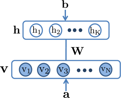
Figure 2: Graphical illustration of a RBM that models the joint distribution of $\mathrm{N}$ visible units and $\mathrm{K}$ hidden units. The connections are undirected and the shaded nodes are observed.

2.1 Model representation

Let $\mathbf{v}$ denote the set of visible variables: $\mathbf{v}=\left[\mathrm{v}_{1},\mathrm{v}_{2},...,\mathrm{v}_{\mathrm{N}}\right]^{\top}\in\left\{0,1\right\}^{\mathrm{N}}$ and $\mathbf{h}$ indicate the set of hidden ones: $\mathbf{h}=\left[\mathrm{h}_{1},\mathrm{h}_{2},...,\mathrm{h}_{\mathrm{K}}\right]^{\top}\in\left\{0,1\right\}^{\mathrm{K}}$. The RBM defines an energy function of a joint configuration $\left(\mathbf{v},\mathbf{h}\right)$ as:

$$E\left(\mathbf{v},\mathbf{h};\psi\right) =-\left(\mathbf{a}^{\top}\mathbf{v}+\mathbf{b}^{\top}\mathbf{h}+\mathbf{v}^{\top}\mathbf{W}\mathbf{h}\right)$$ (1)

where $\psi=\left\{\mathbf{a}\mathbf{,}\mathbf{b},\mathbf{W}\right\}$ is the set of parameters. $\mathbf{a}=\left[\mathrm{a}_{n}\right]_{\mathrm{N}}\in\mathbb{R}^{\mathrm{N}},\mathbf{b}=\left[\mathrm{b}_{k}\right]_{\mathrm{K}}\in\mathbb{R}^{\mathrm{K}}$ are the biases of hidden and visible units respectively, and $\mathbf{W}=\left[\mathrm{w}_{nk}\right]_{\mathrm{N}\times\mathrm{K}}\in\mathbb{R}^{\mathrm{N}\times\mathrm{K}}$ represents the weights connecting the hidden and visible units. The model assigns a Boltzmann distribution (also known as Gibbs distribution) to the joint configuration as:

$$p\left(\mathbf{v},\mathbf{h};\psi\right) =\frac{1}{\mathcal{Z}\left(\psi\right)}e^{-E\left(\mathbf{v},\mathbf{h};\psi\right)}$$ (2)

where $\mathcal{Z}\left(\psi\right)$ is the normalization constant, computed by summing over all possible states pairs of visible and hidden units:

$$\mathcal{Z}\left(\psi\right) =\sum_{\mathbf{v},\mathbf{h}}e^{-E\left(\mathbf{v},\mathbf{h};\psi\right)}$$

Since the network has no intra-layer connections, the Markov blanket of each unit contains only the units of the other layer. Units in one layer become conditionally independent given the other layer. Thus the conditional distributions over visible and hidden units are nicely factorized as:

$$p\left(\mathbf{v}\mid\mathbf{h};\psi\right) =\prod_{n=1}^{\mathrm{N}}p\left(\mathrm{v}_{n}\mid\mathbf{h};\psi\right)$$ (3)

$$p\left(\mathbf{h}\mid\mathbf{v};\psi\right) =\prod_{k=1}^{\mathrm{K}}p\left(\mathrm{h}_{k}\mid\mathbf{v};\psi\right)$$ (4)

wherein the conditional probabilities of single units being active are:

$$p\left(\mathrm{v}_{n}=1\mid\mathbf{h};\psi\right) =\textrm{sig}\left(\mathrm{a}_{n}+\mathbf{w}_{n\raisebox{-1.50694pt}{\scalebox{1.5}{$\cdot$}}}\mathbf{h}\right)$$

$$p\left(\mathrm{h}_{k}=1\mid\mathbf{v};\psi\right) =\textrm{sig}\left(\mathrm{b}_{k}+\mathbf{v}^{\top}\mathbf{w}_{\raisebox{-1.50694pt}{\scalebox{1.5}{$\cdot$}}k}\right)$$ (5)

with the logistic sigmoid function $\textrm{sig}\left(x\right)=\left[1+e^{-x}\right]^{-1}$.

2.2 Parameter learning

The parameter learning of RBM is performed by maximizing the following data log-likelihood:

$$\mathcal{L}\left(\mathbf{v};\psi\right) =\log p\left(\mathbf{v};\psi\right)=\log\sum_{\mathbf{h}}p\left(\mathbf{v},\mathbf{h};\psi\right)$$

The parameters are updated using stochastic gradient ascent as follows:

$$\mathrm{w}_{nk} \leftarrow\mathrm{w}_{nk}+\eta\left(\mathbb{E}_{\tilde{p}}\left[\mathrm{v}_{n}\mathrm{h}_{k}\right]-\mathbb{E}_{p}\left[\mathrm{v}_{n}\mathrm{h}_{k}\right]\right)$$

wherein $\eta>0$ is the learning rate, $\tilde{p}\left(\mathbf{v},\mathbf{h};\psi\right)=\tilde{p}\left(\mathbf{v};\psi\right)p\left(\mathbf{h}\mid\mathbf{v};\psi\right)$ is the data distribution with $\tilde{p}\left(\mathbf{v};\psi\right)$ representing the empirical distribution, $p\left(\mathbf{v},\mathbf{h};\psi\right)$ is the model distribution defined in Eq. (2). Whilst the data expectation $\mathbb{E}_{\tilde{p}}\left[\raisebox{-2.15277pt}{\scalebox{1.5}{$\cdot$}}\right]$ can be computed efficiently, the model expectation $\mathbb{E}_{p}\left[\raisebox{-2.15277pt}{\scalebox{1.5}{$\cdot$}}\right]$ is intractable. To overcome this shortcoming, we use a truncated MCMC-based method known as contrastive divergence (CD) hinton_neucom02_cd to approximate the model expectation. This approximation approach is efficient since the factorizations in Eqs. (3,4) allow fast layer-wise sampling.

2.3 Representation learning

Once the model is fully specified, the new representation of an input data can be achieved by computing the posterior vector $\hat{\mathbf{h}}=\left[\hat{\mathrm{h}}_{1},\hat{\mathrm{h}}_{2},...,\hat{\mathrm{h}}_{\mathrm{K}}\right]$, where $\hat{\mathrm{h}}_{\mathrm{K}}$ is shorthand for $p\left(\mathrm{h}_{k}=1\mid\mathbf{v};\psi\right)$ as given in Eq. (5).

3 Nonnegative restricted Boltzmann machine

We now present our main contribution – the nonnegative restricted Boltzmann machine (NRBM) that integrates nonnegativity into the connection weights of the model. We then present the capability of NRBM to estimate the intrinsic dimensionality of the data, and to stabilize linear predictive models.

3.1 Deriving parts-based representation

The derivation of parts-based representation starts from the connection weights of the standard RBM. In the RBM, two layers are connected using a weight matrix $\mathbf{W}=\left[\mathrm{w}_{nk}\right]_{\mathrm{N}\times\mathrm{K}}$ in which $\mathrm{w}_{nk}$ is the association strength between the hidden unit $k$ and the visible unit $n$. The column vector $\mathbf{w}_{\raisebox{-1.50694pt}{\scalebox{1.5}{$\cdot$}}k}$ is the learned filter of the hidden unit $k$. Parts-based representations imply that this column vector must be sparse, e.g. only a small portion of entries is non-zeros. Recall that the activation of this hidden unit, also known as the firing rate in neural network language, is the probability: $p\left(\mathrm{h}_{k}=1\mid\mathbf{v};\psi\right)=\sigma\left(\mathrm{b}_{k}+\sum_{n=1}^{\mathrm{N}}\mathrm{w}_{nk}\mathrm{v}_{n}\right)$. The positive connection weights tend to activate the associated hidden units whilst the negative turn the units off. In addition, the positive weights add up to representations whereas the negative subtract. Thus it is hard to determine which factors primarily contribute to the learned filter.

Due to asymmetric parameter initialization, the learning process tends to increase some associations more than others. Under nonnegative weights, i.e. $\mathrm{w}_{nk}\geq 0$, the hidden and visible units tend to be more co-active. One can expect that for a given activation probability $\hat{\mathrm{h}}_{k}$ and bias $\mathrm{b}_{k}$, such increase must cause other associations to degrade, since $\mathrm{v}_{n}\geq 0$. As the lower bounds of weights are now zeros, there is a natural tendency for many weights to be driven to zeros as the learning progresses. For an illustration, Fig. 3 shows the histograms of model’s weights at initialization (epoch $\#0$) and learned at epoch $\#1$ and $\#2$. It can be seen that, the number of weights close to zeros increases after each learning epoch.

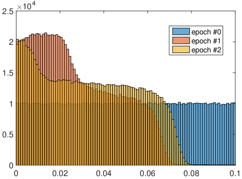
Figure 3: The histograms of NRBM’s weights at the initialization (epoch $\#0$) and learned at epoch $\#1$ and $\#2$.

Recall that learning in the standard RBM is usually based on maximizing the data likelihood with respect to the parameter $\psi$ as:

$$\mathcal{L}\left(\mathbf{v};\psi\right) =p\left(\mathbf{v};\psi\right)=\sum_{\mathbf{h}}p\left(\mathbf{v},\mathbf{h};\psi\right)$$ (6)

To encourage nonnegativity in $\mathbf{W}$, we integrate a nonnegative constraint under quadratic barrier function nocedal_wright_springer99_numerical into the learning of the standard RBM. The objective function now turns into the following regularized log-likelihood:

$$\mathcal{L}_{\textrm{reg}} =\log\mathcal{L}\left(\mathbf{v};\psi\right)-\frac{\alpha}{2}\sum_{n=1}^{\mathrm{N}}\sum_{k=1}^{\mathrm{K}}f\left(\mathrm{w}_{nk}\right)$$ (7)

where:

$$f\left(\mathrm{x}\right) =\begin{cases}\mathrm{x}^{2}&\mathrm{x}<0\\ 0&\mathrm{x}\geq 0\end{cases}$$

and $\alpha\geq 0$. The penalty of sum squared of negative weights regularizes the optimization to encourage nonnegativity in $\mathbf{W}$. The learning procedure now performs minimizing the penalty term and maximizing the data log-likelihood $\log\mathcal{L}\left(\psi;\mathbf{v}\right)$ simultaneously to achieve the optimal solution for the regularized function. The degree of nonnegativity is controlled by the hyperparameter $\alpha$. If we set $\alpha$ to zero, the barrier function will vanish and the model will revert to the ordinary RBM without nonnegative constraint. The larger $\alpha$ is, the tighter the barrier restriction becomes.

Finally the parameter update rule reads:

$$\mathrm{w}_{nk}\leftarrow\mathrm{w}_{nk}+\eta\left(\left\langle\mathrm{v}_{n}\mathrm{h}_{k}\right\rangle_{\tilde{p}}-\left\langle\mathrm{v}_{n}\mathrm{h}_{k}\right\rangle_{p}-\alpha\left\lceil\mathrm{w}_{nk}\right\rceil^{-}\right)$$ (8)

where $\eta>0$ is the learning rate, $\tilde{p}\left(\mathbf{v},\mathbf{h};\psi\right)=\tilde{p}\left(\mathbf{v};\psi\right)p\left(\mathbf{h}\mid\mathbf{v};\psi\right)$ is the data distribution with $\tilde{p}\left(\mathbf{v};\psi\right)$ representing the empirical distribution, $p\left(\mathbf{v},\mathbf{h};\psi\right)$ is the model distribution defined in Eq. (2) and $\left\lceil\mathrm{w}_{nk}\right\rceil^{-}$ denotes the negative part of the weight. Following the learning of standard RBMs hinton_neucom02_cd , $\tilde{p}\left(\mathbf{v};\psi\right)$ is computed from data observations and $p\left(\mathbf{v},\mathbf{h};\psi\right)$ can be efficiently approximated by running multiple Markov short chains starting from observed data at each update.

3.2 Estimating intrinsic dimensionality

The fundamental question of the RBM is how many hidden units are enough to model the data. Currently, no easy methods determine the appropriate number of hidden units needed for a particular problem. One often uses a plentiful number of units, leading to some units are redundant. Note that the unused hidden units problem of RBM is not uncommon which has been studied in berglund_etal_iconip13_measuring . If the number of hidden units is lower than the number of data features, the RBM plays a role of a dimensionality reduction tool. This suggests one prominent method – principal component analysis (PCA) which captures the data variance using the principal components. The amount of variance, however, can help the method specify the number of necessary components. The nonnegativity constraint in the NRBM, interestingly, leads to a similar capacity by examining the “dead” hidden units.

To see how, recall that the hidden and visible units are co-active via the connection weights:

$$p\left(\mathrm{v}_{n}=1\mid\mathbf{h}\right) =\sigma\left(\mathrm{a}_{n}+\sum_{k=1}^{\mathrm{K}}\mathrm{w}_{nk}\mathrm{h}_{k}\right)$$ (9)

Since this probability, in general, is constrained by the data variations, the hidden units must “compete” with each other to explain the data. This is because the contribution towards the explanation is nonnegative, thus an increase on the power of one unit must be at the cost of others. If $\mathrm{K}^{*}<\mathrm{K}$ hidden units are intrinsically enough to account for all variations in the data, then one can expect that either the other $\mathrm{K}-\mathrm{K}^{*}$ hidden units are always deactivated (e.g. with very large negative biases) or their connection weights are almost zeros since $\mathrm{w}_{nk}\geq 0$. In either cases, the hidden units become permanently inoperative in data generation. Thus by examining the dead units, we may be able to uncover the intrinsic dimensionality of the data variations.

4 Stabilizing Linear Predictive Models

This section presents an application of NRBM in stabilizing linear predictive models. Model stability is often overlooked in prediction models which pay more attention to predictive performances. However, model stability is as important as the prognosis in domains where model parameters are interpreted by humans and are subject to external validation. Particularly, in the medical domain, the model stability increases reliability, interpretability, generalization (or transferability) and reproducibility awada_etal_iri12_review ; khoshgoftaar_etal_iri13_survey . For example, it is desirable to have a reliable model that can discover a stable set of risk factors to interpret the causes of the disease. The generalization of the method is the capability to transfer knowledge from one disease to another. This also helps to improve clinical adoption. Finally, stability enables researchers to reproduce the results easily.

A popular modern method to learn predictive risk factors from a high-dimensional data is to employ $\ell_{1}$-penalty, following the success of lasso in linear regression. Lasso is a sparse linear predictive model which promotes feature shrinkage and selection tibshirani_jrss96_regression . More formally, let $\mathbf{X}=\left[\mathrm{x}_{mn}\right]_{\mathrm{M}\times\mathrm{N}}\in\mathbb{R}^{\mathrm{M}\times\mathrm{N}}$ denote the data matrix consisting of $\mathrm{M}$ data points with $\mathrm{N}$ features and $\mathbf{y}=\left[\mathrm{y}_{1},\mathrm{y}_{2},...,\mathrm{y}_{\mathrm{M}}\right]^{\top}\in\left\{0,1\right\}^{\mathrm{M}}$ denote the labels. Consider a predictive distribution:

$$p\left(\mathrm{y}\mid\mathbf{x};\mathbf{w}\right) =p\left(\mathrm{y}\mid\sum_{n=1}^{\mathrm{N}}\mathrm{w}_{n}\mathrm{x}_{n}\right)$$ (10)

Lasso-like learning optimizes a $\ell_{1}$-penalized log-likelihood:

$$\mathcal{L}_{\textrm{lasso}} =\frac{1}{\mathrm{M}}\sum_{m=1}^{\mathrm{M}}\log p\left(\mathrm{y}_{m}\mid\mathbf{x}_{m\raisebox{-1.50694pt}{\scalebox{1.5}{$\cdot$}}};\mathbf{w}\right)-\beta\left\|\mathbf{w}\right\|_{1}$$ (11)

in which $\mathbf{w}=\left[\mathrm{w}_{n}\right]_{\mathrm{N}\times 1}$ is the parameter vector and $\beta>0$ is the regularization hyperparameter. The regularization induces the sparsity of weight vector $\mathbf{w}$.

The lasso, however, is susceptible to data variations (e.g. resampling by bootstrapping, slight perturbation), resulting in loss of stability austin_tu_2004_automated ; xu_etal_pami12_sparse . The method often chooses one of two highly correlated features, resulting in only a 0.5 chance for strongly predictive feature pairs. To overcome this problem, our solution is to provide the lasso with lower-dimensional data representations whose features are expected to be less correlated. Here we introduce a two-stage framework which is a pipeline with the NRBM followed by the lasso. The first stage is to learn the connection weights $\mathbf{W}=\left[\mathrm{w}_{nk}\right]_{\mathrm{N}\times\mathrm{K}}$ of NRBM. Then the machine can map the data onto new representations, i.e. the hidden posteriors: $\mathbf{X}=\left[\mathrm{x}_{mn}\right]_{\mathrm{M}\times\mathrm{N}}\mapsto\hat{\mathbf{X}}=\left[\hat{\mathrm{x}}_{mk}\right]_{\mathrm{M}\times\mathrm{K}}$ (cf. Eq. (5)). The representations are in $\mathrm{K}$-dimensional space and used as the new data for the lasso. At the second stage, the shrinkage method learns $\mathrm{K}$ weights for $\mathrm{K}$ features (i.e. hidden units) to predict the label. Suppose we obtain weight vector $\hat{\mathbf{w}}=\left[\hat{\mathrm{w}}_{1},\hat{\mathrm{w}}_{2},...,\hat{\mathrm{w}}_{\mathrm{K}}\right]^{\top}$, we have:

$$p\left(\mathrm{y}\mid\hat{\mathbf{\mathbf{x}}};\hat{\mathbf{w}}\right) =p\left(\mathrm{y}\mid\sum_{k=1}^{\mathrm{K}}\hat{\mathrm{w}}_{k}\hat{\mathrm{x}}_{k}\right)$$

$$=p\left(\mathrm{y}\mid\sum_{k=1}^{\mathrm{K}}\hat{\mathrm{w}}_{k}\sum_{n=1}^{\mathrm{N}}\mathrm{x}_{n}\mathrm{w}_{nk}\right)$$

$$=p\left(\mathrm{y}\mid\sum_{n=1}^{\mathrm{N}}\mathrm{x}_{n}\sum_{k=1}^{\mathrm{K}}\hat{\mathrm{w}}_{k}\mathrm{w}_{nk}\right)$$

It can be seen that we can sum over the multiplications of the weights of two methods to obtain a new weight vector $\bar{\mathbf{w}}=\left[\bar{\mathrm{w}}_{1},\bar{\mathrm{w}}_{2},...,\bar{\mathrm{w}}_{\mathrm{N}}\right]^{\top}$ as below:

$$\bar{\mathrm{w}}_{n} =\sum_{k=1}^{\mathrm{K}}\hat{\mathrm{w}}_{k}\mathrm{w}_{nk}$$ (12)

These weights connect original features to the label as the weights of lasso in Eq. (10). Thus they can be used to assess the stability of our proposed framework.

5 Experiments

In this section, we quantitatively evaluate the capacity of our proposed model – nonnegative RBM on three applications:

• Parts-based discovery: unsupervised decomposing images into parts, discovering semantic features from texts, and grouping clinically relevant features;

• Feature extraction for classification: discovering discriminative features that help supervised classification; and

• Linear predictive model stabilization: stabilizing feature selection towards rehospitalization prognosis.

We use five real-world datasets in total: three for images, one for text and one for medical data. Three popular image datasets are: one for handwritten digits – MNIST lecun_etal_mnist and two for faces – CBCL mit_cbcl and ORL att_orl . For these datasets, our primary target is to decompose images into interpretable parts (and receptive fields), e.g. dots and strokes in handwritten digits, and facial components in faces. The text corpus is $30$ categories subset of the TDT2 corpus. The goal is to discover plausible latent thematic features, which are groups of semantically related words. Lastly, the medical data is a collection of heart failure patients provided by Barwon Health, a regional health service provider in Victoria, Australia. We aim to investigate the feature stability during the rehospitalization prediction of patients. For prognosis, we use logistic regression model, i.e, $p\left(\mathrm{y}\mid\mathbf{x};\mathbf{w}\right)$ in Eq. (10) is now the probability mass function of a Bernoulli distribution, for 6-month readmission after heart failure.

Image datasets

The MNIST dataset consists of $60,000$ training and $10,000$ testing $28\times 28$ images, each of which contains a handwritten digit. The CBCL database contains facial and non-facial images wherein our interest is only on $2,429$ facial images in the training set. The images are histogram equalized, cropped and rescaled to a standard form of $19\times 19$. Moreover, the human face in each image is also well-aligned. By contrast, the facial images of an individual subject in ORL dataset are captured under a variety of illumination, facial expressions (e.g. opened or closed eyes, smiling or not) and details (e.g. glasses, beard). There are $10$ different images for each of $40$ distinct people. Totally, the data consists of $400$ images with the same size of $92\times 112$ pixels. Images of the three datasets are all in the grayscale whose pixel values are then normalized into the range $[0,1]$. Since the image pixels are not exactly binary data, following the previous work hinton_salakhutdinov_sci06_reducing , we treat the normalized intensity as empirical probabilities on which the NRBM is naturally applied. As the empirical expectation $\left\langle\mathrm{v}_{n}\mathrm{h}_{k}\right\rangle_{\tilde{p}}$ in Eq. (8) requires the probability $p\left(\mathbf{v};\psi\right)$, the normalized intensity is a good approximation.

Text dataset

The TDT2 corpus is collected during the first half of $1998$ from six news sources: two newswires (APW, NYT), two radio programs (VOA, PRI), and two television programs (CNN, ABC). It contains $11,201$ on-topic documents arranged into $96$ semantic categories. Following the preprocessing in cai_etal_tkde05_document , we remove all multiple category documents and keep the largest $30$ categories. This retains $9,394$ documents and $36,771$ unique words in total. We further the preprocessing of data by removing common stopwords. Only $1,000$ most frequent words are then kept and one blank document are removed. For NRBM, word presence is used rather than their counts.

Heart failure data

The data is collected from the Barwon Health which has been serving more than $350,000$ residents. For each time of hospitalization, patient information is recorded into a database using the MySQL server of the hospital. Each record contains patient admissions and emergency department (ED) attendances which form an electronic medical record (EMR). Generally, each EMR consists of demographic information (e.g. age, gender and postcode) and time-stamped events (e.g. hospitalizations, ED visits, clinical tests, diagnoses, pathologies, medications and treatments). Specifically, it includes international classification of disease 10 (ICD-10) scheme WHO_ICD-10 , Australian invention coding (ACHI) scheme ACHI7 , diagnosis-related group (DRG) codes, detailed procedures and discharge medications for each admission and ED visit. Ethics approval was obtained from the hospital and research ethics committee at Barwon Health (number 12/83) and Deakin University.

For our study, we collect the retrospective data of heart failure patients from the hospital’s database. The resulting cohort contains $1,405$ unique patients with $1,885$ admissions between January 2007 and December 2011. We identify patients as heart failure if they had at least one ICD-10 diagnosis code I50 at any admission. Patients of all age groups are included whilst inpatient deaths are excluded from our cohort. Among these patients, $49.3\%$ are male and the medium age is $81.5$ at the time of admission. We focus our study on emergency attendances and unplanned admissions of patients. The readmission of patients is defined as an admission within the horizons of 1, 6 and 12 months after the prior discharge date. After retrieving the data, we follow the one-sided convolutional filter bank method introduced in tran_etal_kdd13_integrated to extract features which are then normalized into the range $\left[0,1\right]$.

To speed up the training phase, we divide training samples into “mini-batches” of $B=100$ samples. Hidden, visible and visible-hidden learning rates are fixed to $0.1$. Visible biases are initialized so that the marginal distribution, when there are no hidden units, matches the empirical distribution. Hidden biases are first set to some reasonable negative values to offset the positive activating contribution from the visible units. Mapping parameters are randomly drawn from positive values in $[0,0.01]$. Parameters are then updated after every mini-batch. Learning is terminated after $100$ epochs. The regularization hyperparameter $\alpha$ in Eq. (7) is empirically tuned so that the data decomposition is both meaningful (e.g. by examining visually, or by computing the parts similarity) and accurate (e.g. by examining the reconstruction quality). The hyperparameter $\beta$ in Eq. (11) is set to $0.001$, which is to achieve the best prediction score.

5.1 Part-based discovery

5.1.1 Decomposing images into parts-based representations

We now show that the nonnegative constraints enable the NRBM to produce meaningful parts-based receptive fields. Fig. 4 depicts the $100$ filters learned from the MNIST images. It can be seen that basic structures of handwritten digits such as strokes and dots are discovered by both RBM and NRBM. However, the features that NRBM learns on Fig. 4b are simpler whilst the ones learned by RBM on Fig. 4a are more difficult to interpret.

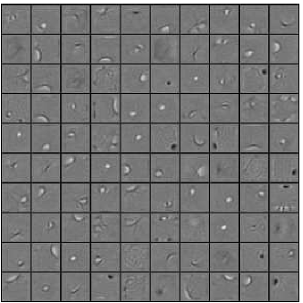
(a) RBM

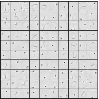
(b) NRBM

Figure 4: Receptive fields learned from the MNIST handwritten digits database using the RBM on Fig. 4a and NRBM on Fig. 4b. Darker pixels illustrate larger weights.

For the CBCL dataset, the facial parts (eyes, mouth, nose, eyebrows etc.) uncovered by NRBM (Fig. 5c) are visually interpretable along the line with classical NMF lee_etal_nature99_nmf (Fig. 5b). The RBM, on the other hand, produces global facial structures (Fig. 5a). On the more challenging facial set with higher variation such as the ORL (cf. Sec. 1), NMF fails to produce parts-based representation (Fig. 1b), and this is consistent with previous findings hoyer_jmlr04_nmf . In contrast, the NRBM is still able to learn facial components (Fig. 1c).

(a) RBM

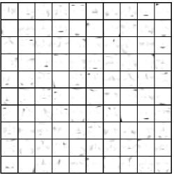
(b) NMF

(c) NRBM

Figure 5: Receptive fields learned from the CBCL face image database using RBM, NMF and NRBM on Figs. (5a,5b,5c). Darker pixels show larger weights.

The capacity to decompose data in NRBM is controlled by a single hyperparameter $\alpha$. As shown in Fig. 6, there is a smooth transition from the holistic decomposition as in standard RBM (when $\alpha$ is near zero) to truly parts-based representations (when $\alpha$ is larger).

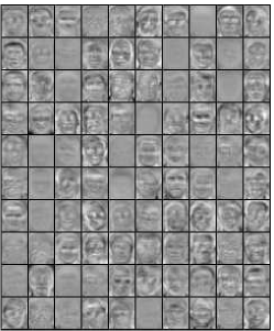
(a) $\alpha=0.001$

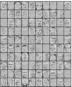
(b) $\alpha=0.01$

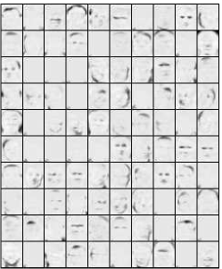
(c) $\alpha=0.1$

Figure 6: Receptive fields learned from the ORL face image database using NRBM with varied barrier costs. The barrier cost $\alpha$ is tightened up from left to right. Darker pixels indicate larger weights.

5.1.2 Dead factors and dimensionality estimation

We now examine the ability of NRBM to estimate the intrinsic dimensionality of the data, as discussed in Section 3.2. We note that by “dimensionality” we roughly mean the degree of variations, not strictly the dimension of the data manifold. This is because our latent factors are discrete binary variables, and thus they may be less flexible than real-valued coefficients.

For that purpose, we compute the number of dead or unused hidden units. The hidden unit $k$ is declared “dead” if the normalized $\ell_{1}$-norm of its connection weight vector is lower than a threshold $\tau$: $\left|\mathbf{w}_{\raisebox{-1.50694pt}{\scalebox{1.5}{$\cdot$}}k}\right|_{1}\mathrm{N}^{-1}\leq\tau$, where $\mathrm{N}$ is the dimension of the original data. We also examine the hidden biases which, however, do not cause dead units in this case. In Fig. 7, the number of used hidden units is plotted against the total number of hidden units $\mathrm{K}$ by taking the average over a set of thresholds ($\tau\in\left\{0.01;0.02;...;0.06\right\}$). With the NRBM, the number of hidden units which explicitly represents the data saturates at about $150$ whilst all units are used by the RBM.

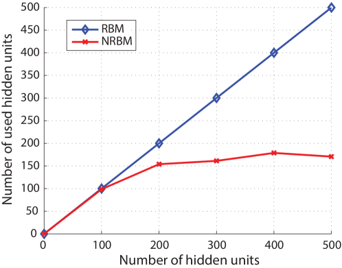
Figure 7: The numbers of used hidden units with different hidden layer sizes of RBM vs NRBM.

5.1.3 Semantic features discovering on text data

The next experiment investigates the applicability of the NRBM on decomposing text into meaningful “parts”, although this notion does not convey the same meaning as those in vision. This is because the nature of text may be more complex and high-level, and it is hard to know whether the true nature of word usage is additive. Following literature in topic modeling (e.g., cf. blei_etal_jmlr03_lda ), we start from the assumption that there are latent themes that govern the choice of words in a particular document. Our goal is to examine whether we can uncover such themes for each document, and whether the themes are corresponding to semantically coherent subset of words.

Using the TDT2 corpus, we learn the NRBM from the data and examine the mapping weight matrix $\mathbf{W}$. For each latent factor $k$, the entry to column $\mathbf{w}_{\raisebox{-1.50694pt}{\scalebox{1.5}{$\cdot$}}k}$ reflects the association strength of a particular word with the factor, where zero entry means distant relation. Table 1 presents four noticeable semantic features discovered by our model. The top row lists the top $15$ words per feature, and the bottom row plots the distribution of association strengths in decreasing order. It appears that the words under each feature are semantically related in a coherent way.

Asian	Current Conflict	1998	India -
Economic Crisis	with Iraq	Winter Olympics	A Nuclear Power?
FINANCIAL	JURY	BUTLER	COURT
FUND	GRAND	RICHARD	BAN
MONETARY	IRAQ	NAGANO	TESTS
INVESTMENT	SEVEN	INSPECTOR	INDIAS
FINANCE	IRAQI	CHIEF	TESTING
WORKERS	GULF	OLYMPICS	INDIA
INVESTORS	BAGHDAD	RISING	SANCTIONS
DEBT	SADDAM	GAMES	ARKANSAS
TREASURY	PERSIAN	COMMITTEE	RULED
CURRENCY	HUSSEIN	WINTER	INDIAN
RATES	KUWAIT	OLYMPIC	PAKISTAN
TOKYO	IRAQS	CHAIRMAN	NUCLEAR
MARKETS	INSPECTOR	JAPANESE	JUDGE
IMF	STANDOFF	EXECUTIVE	LAW
ASIAN	BIOLOGICAL	JAKARTA	ARMS

Table 1: An example of $4$ most distinguished categories, i.e. economics, politics, sport and armed conflict associated with top $15$ words (ranked by their weights) discovered from the TDT2 subset. The charts at the bottom row illustrate the weight impact of words on the category. These weights are sorted in descending order.

5.2 Feature extraction for classification

Our next target is to evaluate whether the ability to decompose data into parts and to disentangle factors of variation could straightforwardly translate into better predictive performance. Although the NRBM can be easily turned into a nonnegative neural network and the weights are tuned further to best fit the supervised setting (e.g., cf. hinton_salakhutdinov_sci06_reducing ), we choose not to do so because our goal is to see if the decomposition separates data well enough. Instead we apply standard classifiers on the learned features, or more precisely the hidden posteriors.

The first experiment is with the MNIST, the $500$ factors have been previously learned in Section 5.1.1 and Fig. 4. Support vector machines (SVM, with Gaussian kernels, using the LIBSVM package chang_etal_tist11_libsvm ) and $k$-nearest neighbors ($k$NN, where $k=4$, with cosine similarity measures) are used as classifiers. For comparison, we also apply the same setting to the features discovered by the NMF. The error rate on test data is reported in Table 2. It can be seen that (i) compared to standard RBM, the nonnegativity constraint used in NRBM does not lead to a degradation of predictive performance, suggesting that the parts are also indicative of classes; and (ii) nonlinear decomposition in NRBM can lead to better data separation than the linear counterpart in NMF.

	SVM	$4$-NN
RBM	1.38	2.74
NMF	3.25	2.64
NRBM	1.4	2.34

Table 2: The classification errors (%) on testing data of MNIST dataset.

The second experiment is on the text data TDT2. Unlike images, words are already conceptual and thus using standard bag-of-words representation is often sufficient for many classification tasks. The question is therefore whether the thematic features discovered by the NRBM could further improve the performance, since it has been a difficult task for topic models such as LDA (e.g., cf. experimental results reported in blei_etal_jmlr03_lda ). To get a sense of the capability to separate data into classes without the class labels, we project the $100$ hidden posteriors onto 2D using t-SNE van_hinton_jmlr08_tsne . Fig. 8a depicts the distribution of documents, where class information is only used for visual labeling. The separation is overall satisfactory.

For the quantitative evaluation, the next step is to run classifiers on learned features. For comparison, we also use those discovered by NMF and LDA. For all models, $100$ latent factors are used, and thus the dimensions are reduced $10$-fold. We split TDT2 text corpus into $80\%$ for training and $20\%$ for testing. We train linear SVMs on all word features and low-dimensional representations provided by LDA, NMF and NRBM with various proportions of training data. Fig. 8b shows the classification errors on testing data for all methods. The learned features of LDA and NMF improve classification performance when training label is limited. This is expected because the learned representations are more compact and thus less prone to overfitting. However, as more labels are available, the word features catch up and eventually outperform those by LDA/NMF. Interestingly, this difficulty does not occur for the features learned by the NRBM, although it does appear that the performance saturates after seeing 20% of training labels. Note that this is significant given the fact that computing learned representations in NRBM is very fast, requiring only a single matrix-vector multiplication per document.

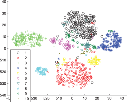
(a) 2D projection of hidden posteriors.

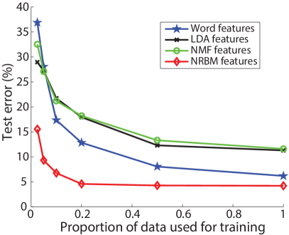
(b) Classification errors $\left(\%\right)$ on TDT2 corpus.

Figure 8: An example visualization of 10 categories and classification performance on TDT2 text corpus. On Fig. 8a, t-SNE projection van_hinton_jmlr08_tsne performs on $100$ higher representations of documents mapped using the NRBM. Categories are labeled using the ground truth. (Best viewed in colors). Fig. 8b represents the classification results for different proportions of training data.

5.3 Stabilizing linear predictive models

In this experiment, we evaluate the stability of feature selection of our framework introduced in Section 4. More specifically, we assess the discovered risk factors of heart failure patients by predicting the future presence of their readmission (i.e., $\mathrm{y}_{m}$ in Eq. (10)) at a certain assessment point given their history. It is noteworthy that this is more challenging as the EMR data contain rich information, are largely temporal, often noisy, irregular, mixed-type, mixed-modality and high-dimensional luo_etal_sdm2012_sor . In what follows, we present the experiment setting, evaluation protocol and results.

5.3.1 Temporal validation

We derive the cohort into training and testing data to validate the predictive performance of our proposed model. Two issues that must be addressed during the splitting process are: learning the past and predicting the future; ensuring training and testing sets completely separated. Here we use a temporal checkpoint to divide the data into two parts. More specifically, we gather admissions which have discharge dates before September 2010 to form the training set and after that for testing. Next we specify the set of unique patients in the training set. We then remove all admissions of such patients in the testing set to guarantee no overlap between two sets. Finally, we obtain $1,088$ unique patients with $1,415$ admissions in the training data and $317$ patients with $360$ admissions in the testing data. The removing steps and resulting datasets are illustrated in Fig. 9. Our model is then learned using training data and evaluated on testing data.

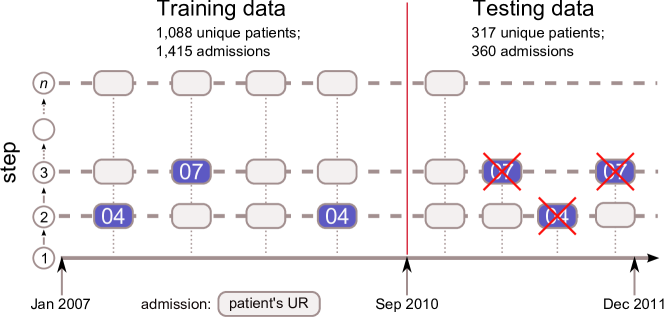
Figure 9: Data splitting process. The cohort was divided into two parts with before September 2010 for training and after that for testing. All admissions of patients in the testing set who are present in training set were then removed to achieve non-overlapping property.

5.3.2 Evaluation protocol

We use Jaccard index real_vargas_1996_probabilistic and consistency index kuncheva_aia07_stability to measure the stability of feature selection process. The Jaccard index, also known as the Jaccard similarity coefficient, naturally considers both similarity and diversity to measure how two feature sets are related. The consistency index supports feature selection in obtaining several desirable properties, i.e. monotonicity, limits and correction for chance.

We trained our proposed model by running $\mathrm{M}=10$ bootstraps and obtained a list of feature sets $\mathcal{S}=\left\{\mathrm{S}_{1},\mathrm{S}_{2},...,\mathrm{S}_{\mathrm{M}}\right\}$ where $\mathrm{S}_{i}$ is a subset of original feature set $\mathbf{v}$. Note that the cardinalities are: $\left|\mathrm{S}_{i}\right|=\mathrm{T}$ and $\left|\mathrm{v}\right|=\mathrm{K}$ with the condition: $\mathrm{T}\leq\mathrm{K}$. Considering a pair of subsets $\mathrm{S}_{i}$ and $\mathrm{S}_{j}$, the pairwise consistency index $C\left(\mathrm{S}_{i},\mathrm{S}_{j}\right)$ is defined as:

$$C\left(\mathrm{S}_{i},\mathrm{S}_{j}\right) =\frac{\mathrm{R}\mathrm{K}-\mathrm{T}^{2}}{\mathrm{T}(\mathrm{K}-\mathrm{T})}$$

in which $\left|\mathrm{S}_{i}\cap\mathrm{S}_{j}\right|=\mathrm{R}$. Taking the average of all pairs, the overall consistency index is:

$$C =\frac{2}{\mathrm{M}(\mathrm{M}-1)}\overset{{}_{\mathrm{M}-1}}{\underset{{}_{i=1}}{\sum}}\overset{{}_{\mathrm{M}}}{\underset{{}_{j=i+1}}{\sum}}C(\mathrm{S}_{i},\mathrm{S}_{j})$$ (13)

Whilst most similarity indices prefer large subsets, $C$ provides consistency around zero for any number of features $\mathrm{T}$ kuncheva_aia07_stability . The consistency index is bounded in $\left[-1,+1\right]$.

Jaccard index measures similarity as a fraction between cardinalities of intersection and union feature subsets. Given two feature sets $\mathrm{S}_{i}$ and $\mathrm{S}_{j}$, the pairwise Jaccard index $J\left(\mathrm{S}_{i},\mathrm{S}_{j}\right)$ reads:

$$J(\mathrm{S}_{i},\mathrm{S}_{j}) =\frac{\left|\mathrm{S}_{i}\cap\mathrm{S}_{j}\right|}{\left|\mathrm{S}_{i}\cup\mathrm{S}_{j}\right|}$$

The Jaccard index evaluating all $\mathrm{M}$ subsets was computed as follows:

$$J =\frac{2}{\mathrm{M}(\mathrm{M}-1)}\overset{{}_{\mathrm{M}-1}}{\underset{{}_{i=1}}{\sum}}\overset{{}_{\mathrm{M}}}{\underset{{}_{j=i+1}}{\sum}}J(\mathrm{S}_{i},\mathrm{S}_{j})$$ (14)

Jaccard index is bounded in $\left[0,1\right]$.

For prediction, we average the weights of $10$ models learned after bootstrapping to obtain the final model. Then the final model performs prediction on testing data. The threshold $0.5$ is used to decide the predicted outcomes from predicted probabilities. Finally the performances are evaluated using measures of sensitivity (recall), specificity, precision, F-measure and area under the ROC curve (AUC) score with confidence intervals based on Mann-Whitney statistic birnbaum_etal_1956_use .

5.3.3 Results

Section 6 shows that the basis matrix of NMF plays the same role as NRBM’s connection weights. Using the same derivation of NRBM in Section 4, it is straightforward to obtain the weight vector $\bar{\mathbf{w}}$ in Eq. (12) for the NMF. Thus we can compare the stability results of our proposed model against those of NMF. In total, we recruit three baselines: lasso, RBM and NMF. The numbers of hidden units, latent factors of RBM, NRBM and NMF are $200$.

Table. 3 reports the prediction performances and Fig. 10 illustrates the stability results for different subset sizes. Overall, the NRBM followed by lasso achieve better AUC score than the RBM and NMF followed by lasso and worse yet acceptable ($1.8\%$ lower) than the sole lasso. However, the NRBM followed by the lasso outperform the sole lasso and RBM$+$Lasso with large margins of consistency and Jaccard indices. The worst stabilities of RBM$+$Lasso are expected because the standard RBM is not designed with properties that promote a steady group of features. Comparing with the NMF followed by lasso, the NRBM performs worse at first but then catches up when the subset size reaches about $150$ and slightly better after that.

Method	Sens./Rec.	Spec.	Prec.	F-mea.	AUC [CI]
Lasso	$0.6137$	$0.5903$	$0.4833$	$0.5404$	$0.6213\left[0.5644,0.6781\right]$
RBM$+$Lasso	$0.5726$	$0.5551$	$0.3944$	$0.4671$	$0.6001\left[0.5425,0.6577\right]$
NMF$+$Lasso	$0.5224$	$0.5536$	$0.5833$	$0.5512$	$0.5690\left[0.5107,0.6274\right]$
NRBM$+$Lasso	$0.5816$	$0.5587$	$0.4011$	$0.4748$	$0.6083\left[0.5508,0.6659\right]$

Table 3: The prediction performance of the NRBM and baselines.

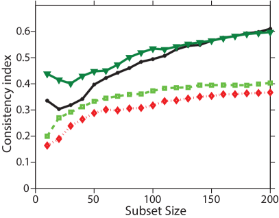
(a) Consistency index.

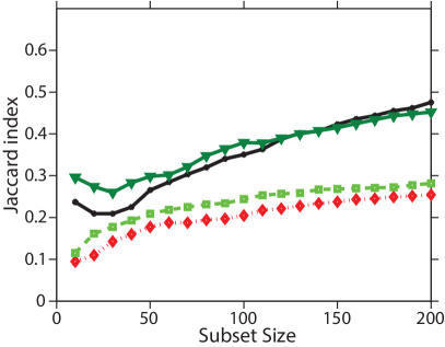
(b) Jaccard index.

Figure 10: Feature selection stability measured by the consistency index (Fig. 10a) and Jaccard index (Fig. 10b) for 6-month heart failure prediction.

6 Discussion

6.1 Representation learning

Representation learning has recently become a distinct area in machine learning after a long time being underneath the subdomain of “feature learning”. This is evidenced through the recent appearance of the international conference on learning representation (ICLR), following a series of workshops in NIPS/ICML bengio_etal_pami13_representation . Existing approaches of learning representation can be broadly classified into three categories: learning kernels, designing hand-crafted features, and learning high-level representations.

In kernel learning approach, the algorithms may use fixed generic kernels such as Gaussian kernel, design kernels based on domain knowledge, or learn combined kernels from multiple base kernels scholkopf_etal_mit99_advances . These methods often use “kernel tricks” to substitute the kernel functions for the mapping functions that transform data into their new representations on the feature space. Thus the kernel machines do not define explicit mapping functions, and as a result do not directly produce representations for data.

The second approach is to directly use either raw data or features extracted from them. These features are extracted from feature selection frameworks with or without domain knowledge. The original data and extracted features can be preprocessed by scaling or normalizing, but not projecting onto other spaces lowe_ijcv04_sift ; dalal_triggs_cvpr05_hog ; oliva_torralba_2006_gist ; bay_etal_eccv06_surf . Normally, the feature selection frameworks are designed by hand. Hand-crafted feature extraction relies on the design of preprocessing pipelines and data transformations. This approach, however, suffers from two significant drawbacks. First, it is labor intensive and normally requires exhaustive prior knowledge. Thus only domain experts can design good features. Second, the feature engineering process may create more data types, especially for complex data, leading to more challenges for fundamental machine learning methods.

The last approach is to automatically learn parametric maps that transform input data into high-level representations. The models that learn such representations typically fall into two classes: one is non-probabilistic models, the other is probabilistic latent variable models. The common aim of the methods in the first class is to learn direct encoding, i.e., parametric maps from input data to their new representations. The classic linear techniques are principal component analysis (PCA) jolliffe_springer86_pca , latent semantic indexing (LSI) deerwester_etal_jasis90_lsi , and independent component analysis (ICA) hyvarinen_oja_nn00_independent . These methods support capturing data regularity, discovering latent structures and latent semantics of data. They, however, face difficulty in modeling data which follow a set of probabilistic distributions. This drawback can be overcome by the second class of probabilistic models.

Probabilistic latent variable models often consist of observed variables $\mathbf{x}$ representing data and latent variables $\mathbf{h}$ which coherently reflect the distributions, regularities, structures and correlations of data. The common idea is to define a joint probability $p\left(\mathbf{x},\mathbf{h}\right)$ over the joint space of observed and latent variables. The learning is to maximize the likelihood of training data. Once the model has been learned, the latent representation of the data is obtained by inferring the posterior probability $p\left(\mathbf{h}\mid\mathbf{x}\right)$. Most methods in this part are probabilistic versions of the ones in the first class including probabilistic PCA tipping_etal_jrss99_pPCA , probabilistic LSI hofmann_uai99_pLSI , and Bayesian nonparametric factor analysis paisley_etal_icml09_bnfa . As a fully generative two-layer model, our proposed model can also be categorized into this class.

6.2 Nonnegative data modeling

Our work was partly motivated by the capacity of nonnegative matrix factorization (NMF) lee_etal_nature99_nmf to uncover parts-based representations. Given a nonnegative data matrix $\mathbf{V}\in\mathbb{R}^{\mathrm{N}\times\mathrm{M}}$, the NMF attempts to factorize into two low-rank real-valued nonnegative matrices, the basis $\mathbf{W}\in\mathbb{R}^{\mathrm{N}\times\mathrm{K}}$ and the coefficient $\mathbf{H}\in\mathbb{R}^{\mathrm{K}\times\mathrm{M}}$, i.e., $\mathbf{V}\approx\mathbf{W}\mathbf{H}$. Thus $\mathbf{W}$ plays the same role as NRBM’s connection weights, and each column of $\mathbf{H}$ assumes the “latent factors”. However, it has been pointed out that unless there are appropriate sparseness constraints or certain conditions, the NMF is not guaranteed to produce parts hoyer_jmlr04_nmf . Our experiment shows, on the contrary, the NRBM can still produce parts-based representation when the NMF fails (Fig. 1, also reported in hoyer_jmlr04_nmf ).

On the theoretical side, the main difference is that, in our cases, the latent factors are stochastic binary that are inferred from the model, but not learned as in the case of NMF. In fact this seemingly subtle difference is linked to a fundamental drawback of the NMF: The learned latent factors are limited to seen data only, and must be relearned for every new data point. The NRBM, on the other hand, is a fully generative model in that it can generate new samples from its distribution, and at the same time, the representations can be efficiently computed for unseen data (cf. Eq. (5)) using one matrix operation.

Recently, there has been work closely related to the NMF that does not require re-estimation on unseen data lemme_etal_nn12_online . In particular, the coefficient matrix $\mathbf{H}$ is replaced by the mapping from the data itself, that is $\mathbf{H}=\boldsymbol{\sigma}\left(\mathbf{W}^{\top}\mathbf{V}\right)$, resulting in the so-called autoencoder structure (AE), that is $\mathbf{V}\approx\mathbf{W}\boldsymbol{\sigma}\left(\mathbf{W}^{\top}\mathbf{V}\right)$, where $\boldsymbol{\sigma}(\boldsymbol{x})$ is a vector of element-wise nonlinear transforms and $\mathbf{W}$ is nonnegative. A new representation estimated using $\boldsymbol{\sigma}\left(\mathbf{W}^{\top}\mathbf{V}\right)$ now plays the role of the posteriors in NRBM, although it is non-probabilistic. The main difference from the NRBM is that the nonnegative AE does not model data distribution, and thus cannot generate new samples. Also, it is still unclear how the new representation could be useful for classification in general and on non-vision data in particular.

6.3 Feature discovery

For the semantic analysis of text, our proposed model is able to discover plausible thematic features. Compared against those discovered by topic models such as latent Dirichlet allocation (LDA) blei_etal_jmlr03_lda , we found that they are qualitatively similar. We note that the two approaches are not directly comparable because the notion of association strength between a latent factor and a word, as captured in the nonnegative weight $\mathrm{w}_{nk}$, cannot be translated into the properly normalized probability $P(\mathrm{v}_{n}=1\mid\mathrm{z}_{n}=k)$ as in LDA, where $\mathrm{z}_{n}$ is the topic that generates the word $\mathrm{v}_{n}$. Nevertheless, the NRBM offers many advantages over the LDA: (i) the notion that each document is generated from a subset of themes (or semantic features) in the NRBM is an attractive alternative to the setting of topic distribution as assumed in the LDA (cf. also griffiths_ghahramani_2005_infinite ); (ii) inference to compute the latent representation given an input is much faster in the NRBM with only one matrix multiplication step, which typically requires an expensive sampling run in the LDA; (iii) learning in the NRBM can be made naturally incremental, whilst estimating parameter posteriors in the LDA generally requires the whole training data; and (iv) importantly, as shown in our experiments, classification using the learned representations can be more accurate with the NRBM.

This work can be considered along the line of imposing structures on standard RBM so that certain regularities are explicitly modeled. Our work has focused on nonnegativity as a way to ensure sparseness on the weight matrix, and consequently the latent factors. An alternative would be enforcing sparseness on the latent posteriors, e.g., hinton_springer12_practical . Another important aspect is that the proposed NRBM offers a way to capture the so-called “explaining away” effect, that is the latent factors compete with each other as the most plausible explanatory causes for the data (cf. also Section 3.2). The competition is encouraged by the nonnegative constraints, as can be seen from the generative model of data $p\left(\mathrm{v}_{n}=1\mid\mathbf{h};\psi\right)=\sigma\left(\mathrm{a}_{n}+\sum_{k}\mathrm{w}_{nk}\mathrm{h}_{k}\right)$, in that some large weights (strong explaining power) will force others to degrade or even vanish (weak explaining power). This is different from standard practice in neural networks, where complex inhibitory lateral connections must be introduced to model the competition hinton_ghahramani_biosci97_generative .

One important question is that under such constraints, besides the obvious gains in structural regularization, do we lose representational power of the standard RBM? On one hand, our experience has indicated that yes, there is certain loss in the ability to reconstruct the data, since the parameters are limited to be nonnegative. On the other hand, we have demonstrated that this does not away translate into the loss of predictive power. In our setting, the degree of constraints can also be relaxed by lowering down the regularization parameter $\alpha$ in Eq. (7), and this would allow some parameters to be negative.

6.4 Model stability

The high-dimensional data necessitates sparse models wherein only small numbers of strongly predictive features are selected. However, most sparsity-inducing algorithms lead to unstable models due to data variations (e.g., resampling by bootstrapping, slight perturbation) xu_etal_pami12_sparse . For example, logistic regression produces unstable models while performing automated feature selection austin_tu_2004_automated . In the context of lasso, the method tends to keep only one feature if two are highly correlated zou_hastie_jrss05_regularization , resulting in loss of stability.

Model stability refers to the consistent degree of model parameters which are learned under data changes. For classifiers with embedded feature selection, a sub-problem is the stability of selected subsets of features. The importance of stability in feature selection has been largely ignored in literature. A popular approach in initial work is to compare feature selection methods basing on feature preferences ranked by their weights kvrivzek_etal_caip07_improving ; kalousis_etal_kais07_stability . Another approach targets on developing a number of metrics to measure stability khoshgoftaar_etal_iri13_survey . Recently, model stability has been studied more widely in bioinformatics. The research focus is to improve the stability by exploiting aggregated information park_etal_biostats07_averaged ; abraham_etal_bmc10_prediction ; soneson_etal_biostats12_framework and the redundancy in the feature set yuan_lin_jrss06_model ; yu_etal_kdd08_stable .

In this paper, our work addresses the stability problem via readmission prognosis of heart failure patients using high-dimensional medical records. The heart failure data is studied in he_etal_jamia13_mining but with only a small subset of features. Our recent work employs graph-based regularization to stabilize linear models gopakumar_etal_jbhi14_stabilizing ; tran_etal_kais14_stabilized . This paper differs from our previous work in that no external information is needed. Rather, it is based on self-organization of features into parts which are more stable than original features. This application in healthcare analytics continues our on going research on modeling electronic medical records which are high-dimensional and heterogeneous data tu_etal_pakdd13_latent .

7 Conclusion

To summarize, this paper has introduced a novel variant of the powerful restricted Boltzmann machine, termed nonnegative RBM (NRBM), where the mapping weights are constrained to be nonnegative. This gives the NRBM the new capacity to discover interpretable parts-based representations, semantically plausible high-level features for additive data such as images and texts. Our proposed method can also stabilize linear predictive models in feature selection task for high-dimensional medical data. In addition, the NRBM can be used to uncover the intrinsic dimensionality of the data, the ability not seen in the standard RBM. This is because under the nonnegativity constraint, the latent factors “compete” with each other to best represent data, leading to some unused factors. At the same time, the NRBM retains nearly full strength of the standard RBM, namely, compact and discriminative distributed representation, fast inference and incremental learning.

Compared against the well-studied parts-based decomposition scheme, the nonnegative matrix factorization (NMF), the NRBM could work in places where the NMF fails. When it comes to classification using the learned representations, the features discovered by the NRBM are more discriminative than those by the NMF and the latent Dirichlet allocation (LDA). For model stability, the performance of the proposed model surpasses the lasso, the RBM and is comparable to the NMF. Thus, we believe that the NRBM is a fast alternative to the NMF and LDA for a variety of data processing tasks.

References

- [1] Gad Abraham, Adam Kowalczyk, Sherene Loi, Izhak Haviv, and Justin Zobel. Prediction of breast cancer prognosis using gene set statistics provides signature stability and biological context. BMC Bioinformatics, 11:277, May 2010.
- [2] Australian Classification Of Health Interventions: ACHI-7th, 2013. Accessed September, 2013.
- [3] Shivani Agarwal, Aatif Awan, and Dan Roth. Learning to detect objects in images via a sparse, part-based representation. IEEE Transactions on Pattern Analysis and Machine Intelligence (PAMI), 26(11):1475–1490, 2004.
- [4] AT&T@Cambridge. The ORL Database of Faces. AT&T Laboratories Cambridge, 2002.
- [5] Peter C Austin and Jack V Tu. Automated variable selection methods for logistic regression produced unstable models for predicting acute myocardial infarction mortality. Journal of Clinical Epidemiology, 57(11):1138–1146, 2004.
- [6] Wael Awada, Taghi M Khoshgoftaar, David Dittman, Randall Wald, and Amri Napolitano. A review of the stability of feature selection techniques for bioinformatics data. In Proceedings of the IEEE 13th International Conference on Information Reuse and Integration (IRI), pages 356–363, Las Vegas, United States, August 8–10 2012.
- [7] Herbert Bay, Tinne Tuytelaars, and Luc Van Gool. Surf: Speeded up robust features. In Proceedings of the 9th European Conference on Computer Vision (ECCV), volume 3951, pages 404–417, Graz, Austria, May 7–13 2006. Springer.
- [8] Yoshua Bengio, Aaron Courville, and Pascal Vincent. Representation learning: A review and new perspectives. IEEE Transactions on Pattern Analysis and Machine Intelligence (PAMI), 35(8):1798–1828, 2013. printed;.
- [9] Mathias Berglund, Tapani Raiko, and KyungHyun Cho. Measuring the usefulness of hidden units in Boltzmann machines with mutual information. In Proceedings of the 20th International Conference on Neural Information Processing (ICONIP), volume 8226, pages 482–489, Daegu, South Korea, November 3–7 2013. Springer.
- [10] ZW Birnbaum et al. On a use of the Mann-Whitney statistic. In Proceedings of the 3rd Berkeley Symposium on Mathematical Statistics and Probability, Volume 1: Contributions to the Theory of Statistics. The Regents of the University of California, 1956.
- [11] David M Blei, Andrew Y Ng, and Michael Jordan. Latent dirichlet allocation. The Journal of Machine Learning Research (JMLR), 3:993–1022, 2003.
- [12] Deng Cai, Xiaofei He, and Jiawei Han. Document clustering using locality preserving indexing. IEEE Transactions on Knowledge and Data Engineering (TKDE), 17(12):1624–1637, December 2005.
- [13] CBCL@MIT. CBCL Face Database. Center for Biological and Computation Learning at MIT, 2000.
- [14] Chih-Chung Chang and Chih-Jen Lin. LIBSVM: A library for support vector machines. ACM Transactions on Intelligent Systems and Technology, 2:27:1–27:27, 2011. Software available at http://www.csie.ntu.edu.tw/~cjlin/libsvm.
- [15] Navneet Dalal and Bill Triggs. Histograms of oriented gradients for human detection. In Proceedings of the IEEE Computer Society Conference on Computer Vision and Pattern Recognition (CVPR), volume 1, pages 886–893, San Diego, United States, June 20–25 2005. IEEE.
- [16] Scott Deerwester, Susan T. Dumais, George W Furnas, Thomas K Landauer, and Richard Harshman. Indexing by latent semantic analysis. Journal of the American Society for Information Science, 41(6):391–407, 1990.
- [17] Yoav Freund and David Haussler. Unsupervised learning of distributions on binary vectors using two layer networks. Technical Report UCSC-CRL-94-25, Baskin Center for Computer Engineering & Information Sciences, University of California Santa Cruz (UCSC), Santa Cruz, CA, USA, 1994.
- [18] Shivapratap Gopakumar, Truyen Tran, T Nguyen, Dinh Phung, and Svetha Venkatesh. Stabilizing high-dimensional prediction models using feature graphs. IEEE Journal of Biomedical and Health Informatics (JBHI), 2014.
- [19] T. Griffiths and Z. Ghahramani. Infinite latent feature models and the Indian buffet process. 2005.
- [20] Danning He, Simon C Mathews, Anthony N Kalloo, and Susan Hutfless. Mining high-dimensional administrative claims data to predict early hospital readmissions. Journal of the American Medical Informatics Association (JAMIA), 21(2):272–279, 2014.
- [21] Geoffrey Hinton and Ruslan Salakhutdinov. Reducing the dimensionality of data with neural networks. Science, 313(5786):504 – 507, 2006.
- [22] Geoffrey E. Hinton. Training products of experts by minimizing contrastive divergence. Neural Computation, 14(8):1771–1800, 2002.
- [23] Geoffrey E. Hinton. A practical guide to training restricted Boltzmann machines. In Neural Networks: Tricks of the Trade, volume 7700 of Lecture Notes in Computer Science, pages 599–619. Springer Berlin Heidelberg, 2012.
- [24] Geoffrey E Hinton and Zoubin Ghahramani. Generative models for discovering sparse distributed representations. Philosophical Transactions of the Royal Society of London. Series B: Biological Sciences, 352(1358):1177–1190, 1997.
- [25] Thomas Hofmann. Probabilistic latent semantic analysis. In Proceedings of the 15th Conference on Uncertainty in Artificial Intelligence (UAI), pages 289–296. Morgan Kaufmann Publishers Inc., July 1999.
- [26] Patrik O Hoyer. Non-negative matrix factorization with sparseness constraints. The Journal of Machine Learning Research, 5:1457–1469, 2004. printed.
- [27] Aapo Hyvärinen and Erkki Oja. Independent component analysis: algorithms and applications. Neural Networks, 13(4):411–430, 2000.
- [28] World Health Organization: ICD-10th, 2010. Accessed September, 2012.
- [29] Ian T Jolliffe. Principal component analysis, volume 487. Springer-Verlag New York, 1986.
- [30] Alexandros Kalousis, Julien Prados, and Melanie Hilario. Stability of feature selection algorithms: a study on high-dimensional spaces. Knowledge and Information Systems (KAIS), 12(1):95–116, 2007.
- [31] Taghi M Khoshgoftaar, Alireza Fazelpour, Huanjing Wang, and Randall Wald. A survey of stability analysis of feature subset selection techniques. In Proceedings of the IEEE 14th International Conference on Information Reuse and Integration (IRI), pages 424–431, San Francisco, United States, August 14–16 2013. IEEE.
- [32] Ludmila I Kuncheva. A stability index for feature selection. In Proceedings of the IASTED International Conference on Artificial Intelligence and Applications (AIA), pages 390–395, Innsbruck, Austria, February 12–14 2007.
- [33] Pavel Kvrivzek, Josef Kittler, and Vaclav Hlavac. Improving stability of feature selection methods. In Proceedings of the 12th International Conference on Computer Analysis of Images and Patterns (CAIP), volume 4673, pages 929–936, Vienna, Austria, August 27–29 2007. Springer.
- [34] Yann Lecun, Corinna Cortes, and Christopher J.C. Burges. The MNIST database of handwritten digits. 1998.
- [35] Daniel D Lee and H Sebastian Seung. Learning the parts of objects by non-negative matrix factorization. Nature, 401(6755):788–791, 1999.
- [36] Andre Lemme, René Felix Reinhart, and Jochen Jakob Steil. Online learning and generalization of parts-based image representations by non-negative sparse autoencoders. Neural Networks, 33(0):194 – 203, 2012.
- [37] David G Lowe. Distinctive image features from scale-invariant keypoints. International Journal of Computer Vision, 60(2):91–110, 2004.
- [38] D. Luo, F. Wang, J. Sun, M. Markatou, J. Hu, and S. Ebadollahi. SOR: Scalable orthogonal regression for non-redundant feature selection and its healthcare applications. In Proceedings of the 12th SIAM International Conference on Data Mining (SDM), pages 576–587, Anaheim, United States, April 26–28 2012.
- [39] Tu Dinh Nguyen, Truyen Tran, Dinh Phung, and Svetha Venkatesh. Latent patient profile modelling and applications with mixed-variate restricted boltzmann machine. In Jian Pei, VincentS. Tseng, Longbing Cao, Hiroshi Motoda, and Guandong Xu, editors, Proceedings of the 17th Pacific-Asia Conference on Knowledge Discovery and Data Mining (PAKDD), volume 7818 of Lecture Notes in Computer Science, pages 123–135, Gold Coast, Australia, 2013. Springer-Verlag Berlin Heidelberg.
- [40] Tu Dinh Nguyen, Truyen Tran, Dinh Phung, and Svetha Venkatesh. Learning parts-based representations with nonnegative restricted Boltzmann machine. In Proceedings of the 5th Asian Conference on Machine Learning (ACML), volume 29, pages 133–148, Canberra, Australia, November 13–15 2013.
- [41] Jorge Nocedal and Stephen J. Wright. Numerical Optimization. Springer, August 2000, pp. 497–506.
- [42] Aude Oliva and Antonio Torralba. Building the gist of a scene: The role of global image features in recognition. Progress in Brain Research, 155:23–36, 2006.
- [43] J. Paisley and L. Carin. Nonparametric factor analysis with beta process priors. In Proceedings of the 26th Annual International Conference on Machine Learning (ICML), pages 777–784, Montreal, Canada, June 14–18 2009. ACM.
- [44] Mee Young Park, Trevor Hastie, and Robert Tibshirani. Averaged gene expressions for regression. Biostatistics, 8(2):212–227, 2007.
- [45] Raimundo Real and Juan M Vargas. The probabilistic basis of Jaccard’s index of similarity. Systematic Biology, 45(3):380–385, 1996.
- [46] Bernhard Schölkopf, Christopher JC Burges, and Alexander J Smola. Advances in kernel methods: support vector learning. MIT press, 1999.
- [47] P. Smolensky. Information processing in dynamical systems: Foundations of harmony theory. In David E. Rumelhart and James L. McClelland, editors, Parallel Distributed Processing: Explorations in the Microstructure of Cognition, volume 1, chapter 6, pages 194–281. MIT Press, 1986.
- [48] Charlotte Soneson and Magnus Fontes. A framework for list representation, enabling list stabilization through incorporation of gene exchangeabilities. Biostatistics, 13(1):129–141, 2012.
- [49] Yee Whye Teh and Geoffrey E Hinton. Rate-coded restricted Boltzmann machines for face recognition. In Proceedings of the 14th Annual Conference on Neural Information Processing Systems (NIPS), pages 908–914, Denver, United States, 2000 November 27 – December 2 2001. MIT.
- [50] Robert Tibshirani. Regression shrinkage and selection via the lasso. Journal of the Royal Statistical Society. Series B (Methodological), pages 267–288, 1996.
- [51] Michael E Tipping and Christopher M Bishop. Probabilistic principal component analysis. Journal of the Royal Statistical Society: Series B (Statistical Methodology), 61(3):611–622, 1999.
- [52] Truyen Tran, Dinh Phung, Wei Luo, Richard Harvey, Michael Berk, and Svetha Venkatesh. An integrated framework for suicide risk prediction. In Proceedings of the 19th ACM SIGKDD International Conference on Knowledge Discovery and Data Mining (KDD), pages 1410–1418, Chicago, USA, August 11–14 2013. ACM.
- [53] Truyen Tran, Dinh Phung, Wei Luo, and Svetha Venkatesh. Stabilized sparse ordinal regression for medical risk stratification. Knowledge and Information Systems (KAIS), pages 1–28, 2014.
- [54] L. van der Maaten and G. Hinton. Visualizing data using t-SNE. The Journal of Machine Learning Research (JMLR), 9(Nov):2579–2605, 2008.
- [55] Huan Xu, Constantine Caramanis, and Shie Mannor. Sparse algorithms are not stable: A no-free-lunch theorem. IEEE Transactions on Pattern Analysis and Machine Intelligence (PAMI), 34(1):187–193, 2012.
- [56] Lei Yu, Chris Ding, and Steven Loscalzo. Stable feature selection via dense feature groups. In Proceedings of the 14th ACM SIGKDD International Conference on Knowledge Discovery and Data Mining (KDD), pages 803–811, Las Vegas, United States, August 24–27 2008. ACM.
- [57] Ming Yuan and Yi Lin. Model selection and estimation in regression with grouped variables. Journal of the Royal Statistical Society: Series B (Statistical Methodology), 68(1):49–67, 2006.
- [58] Hui Zou and Trevor Hastie. Regularization and variable selection via the elastic net. Journal of the Royal Statistical Society: Series B (Statistical Methodology), 67(2):301–320, 2005.