Statistical Latent Space Approach for Mixed Data Modelling and Applications

Abstract

The analysis of mixed data has been raising challenges in statistics and machine learning. One of two most prominent challenges is to develop new statistical techniques and methodologies to effectively handle mixed data by making the data less heterogeneous with minimum loss of information. The other challenge is that such methods must be able to apply in large-scale tasks when dealing with huge amount of mixed data. To tackle these challenges, we introduce parameter sharing and balancing extensions to our recent model, the mixed-variate restricted Boltzmann machine (MV.RBM) which can transform heterogeneous data into homogeneous representation. We also integrate structured sparsity and distance metric learning into RBM-based models. Our proposed methods are applied in various applications including latent patient profile modelling in medical data analysis and representation learning for image retrieval. The experimental results demonstrate the models perform better than baseline methods in medical data and outperform state-of-the-art rivals in image dataset.

Pattern Recognition and Data Analytics
School of Information Technology, Deakin University, Australia.
Locked Bag 20000, Geelong VIC 3220, Australia.
Tel: +61 3 5227 2150
Internal report number: TR-PRaDA-05/13, May, 2013.

Statistical Latent Space Approach for Mixed Data Modelling and Applications

Tu Dinh Nguyen$\dagger$, Truyen Tran$\dagger$$\ddagger$, Dinh Phung$\dagger$ and Svetha Venkatesh$\dagger$

$\dagger$Center for Pattern Recognition and Data Analytics

School of Information Technology, Deakin University, Geelong, Australia

$\ddagger$Institute for Multi-Sensor Processing and Content Analysis

Curtin University, Australia

Email: {ngtu,truyen.tran,dinh.phung,svetha.venkatesh}@deakin.edu.au

1 Introduction

Data can be collected from numerous sources such as cameras, sensors, human opinions, user preferences, recommendations, ratings, moods, which together are called multisource. Such data can also exist in any forms of text, hypertext, image, graphics, video, speech and audio, namely multimodality. Data also vary in types (e.g., binary, categorical, multicategorical, continuous, ordinal, count, rank) which are known as multitype. The combination of multisource, multimodality and multitype has created mixed data with the characteristics of complexity and heterogeneity. Nowadays the advances of information technology has enabled seemingly limitless collection, archive and retrieval of data, leading to an enormous amount of mixed data. Such huge databases are useful only if they are analysed to reveal their latent trends, internal dependencies and structures. Therefore, it is imperative to develop new statistical techniques and methodologies to effectively handle mixed data. However, the challenges arise in such tasks are manifolds. One of the two most prominent challenges is that no simple scaling and transforming methods can make data less heterogeneous without distorting them. The other challenge is that the analysis method must be scalable to meet the requirements of computational complexity and timing when dealing with huge amount of mixed data. There have been three main research directions to analyse mixed data as follows:

• Directly applying machine learning techniques without transforming the data. In this approach, machine learning methods perform on either raw data or features extracted from them. Note that these features are extracted from feature selection frameworks with or without prior knowledge. Original data and extracted features can be preprocessed by scaling or normalising, but not projecting to other spaces.

• Non-probabilistically transforming data to higher-level representations before performing machine learning methods. Here, researchers use several methods (e.g., dimensionality reduction techniques) to transform raw data or features extracted from them into another space. The projected data on this new space are called higher-level representations of the original data. These representations are then fed into machine learning methods for final processing. However, widely-used transformation methods usually perform in linear fashion without integrating probabilistic properties.

• Modelling mixed data using latent variable frameworks. In this case, probabilistic graphical models are constructed with latent and observed variables which are obtained from data. These models define joint distribution over all variables or conditional distribution of latent variables given observed ones. After that, they can discover latent representations for the data by computing the conditional probabilities of latent variables given observed ones. Machine learning methods then can be applied to these latent representations, similarly to higher-level representation in the second approach above. Meanwhile, some latent variable models are highly flexible. They can do classification, regression, data completion, prediction or even visualisation without further processing [81].

The significant drawback of the first approach is that almost fundamental methods are only able to handle univariate data or correlation among a few features at the same time. Some of them can perform on the combination (e.g., merely concatenated feature vectors) of multiple features but provide poor results. More interestingly, there are still several methods which can simultaneously treat multiple types of data separately and then form a fusion at a certain stage. However, the fusion fails to either flexibly tackle with each type or capture inter-feature relations. The second approach supports understanding data distributions, discovering latent structures and latent semantics of data. Unfortunately, it still depends on the fusion of higher-level representations when dealing with mixed data. By contrast, models in the last approach state their outstanding performances. They simultaneously model multiple types and modalities in probabilistic sense, uncover latent structures and factors of data, and even efficiently do further machine learning tasks by themselves. According to these reasons, we propose our models following the last approach.

The rest of technical report is organised as follows. The next section explains three main approaches to analyse mixed data by reviewing typical literature on such approaches. We then describe our approach and modelling frameworks in Section 3. Next, Section 4 presents the applications of our models on real datasets. We then discuss about several drawbacks of our model and build future research plans to overcome those hurdles in Section 5. Finally, Section 6 concludes the report.

2 Mixed Data Analysis: An overview

In this section, we present a literature review on three main approaches of mixed data analysis. Firstly, we briefly revise several applications with multitype and multimodality data using the first and second approach, i.e., using original features and mapping to higher-level representations. Then we focus on the third approach of using latent variable graphical models for mixed data modelling.

2.1 Original features

Most existing machine learning methods are restricted to handle univariate data or correlation among a few features. They are often theoretically designed to deal with single type and modality of data at the same time. However, there are still several methods which can simultaneously treat multiple types and modalities of data separately and then form a fusion at a certain stage. Some of the most considerable include Support Vector Machines (SVMs) and Neural Networks. Here, for example, we will explain about the SVMs in more detail.

Support Vector Machines (SVMs) [12, 6] are a widely-used machine learning method for classification, regression and other tasks. The SVMs have shown their capabilities in pattern recognition such as handwritten digit recognition, object recognition, speaker identification, face detection, face recognition and text categorisation. The method aims to find the optimal hyperplane to separate relevant and irrelevant samples. The optimisation is done by maximising the margin between both sets of samples. Note that the optimisation idea of SVMs lays the foundation for the development of new approaches including large-margin methods, distance metric learning and regularisation techniques [65].

Let $\mathcal{D}=\left\{\left(\boldsymbol{x}_{i},y_{i}\right)\right\}$ denote the training set containing instance-label pairs $\left(\boldsymbol{x}_{i},y_{i}\right)$ with $i=1,...,N$ in which $\boldsymbol{x}_{i}$ is $n$-dimensional vector, i.e., $\boldsymbol{x}_{i}\in\mathbb{R}^{n}$, and $y_{i}$ has indicator value, i.e., $y_{i}\in\left\{1,-1\right\}$. The SVMs attempt to look for the solution of following optimisation problem

$$\min_{\boldsymbol{w},b,\boldsymbol{\xi}} \frac{1}{2}\boldsymbol{w}^{\top}\boldsymbol{w}+C\sum_{i=1}^{N}\xi_{i}$$

subject to $$y_{i}\left(\boldsymbol{w}^{\top}\phi\left(\boldsymbol{x}_{i}\right)+b\right)\geq 1-\xi_{i},$$

$$\xi_{i}\geq 0.$$

where $\phi$ is the mapping function, $\boldsymbol{\xi}$ are error terms and $C>0$ is the penalty parameter of the error terms. The training sample $\boldsymbol{x}_{i}$ is mapped into another space. The transformation here can be non-linear and the projected space maybe higher or even infinite dimensionality. Therefore, although the separator, i.e., separating hyperplane, is linear in high-dimensional space, it possibly is non-linear in the original one. Denote by $K\left(\boldsymbol{x}_{i},\boldsymbol{x}_{j}\right)=\phi\left(\boldsymbol{x}_{i}\right)^{\top}\phi\left(\boldsymbol{x}_{i}\right)$ the kernel function. So far, there have been numerous kernels for individual problem or category of data. Four basic kernels should be mentioned as below

• Linear kernel: $K\left(\boldsymbol{x}_{i},\boldsymbol{x}_{j}\right)=\boldsymbol{x}_{i}^{\top}\boldsymbol{x}_{j}+c$ where $c$ is an optional constant. The linear kernel is the simplest kernel function basing on the inner product $\left\langle\boldsymbol{x}_{i},\boldsymbol{x}_{j}\right\rangle$.

• Polynomial kernel: $K\left(\boldsymbol{x}_{i},\boldsymbol{x}_{j}\right)=\left(\gamma\boldsymbol{x}_{i}^{\top}\boldsymbol{x}_{j}+r\right)^{d}$ in which $r$ is the constant, $d$ is polynomial degree, $\gamma>0$ is the slope parameter. This kernel is appropriate to the data which can be normalised.

• Sigmoid kernel: $K\left(\boldsymbol{x}_{i},\boldsymbol{x}_{j}\right)=\tanh\left(\alpha\boldsymbol{x}_{i}^{\top}\boldsymbol{x}_{j}+c\right)$ with $\alpha$ is the slope parameter and $c$ is the intercept constant. This kernel is also known as Hyperbolic Tangent kernel and Multilayer Perceptron (MLP) kernel. MLP reminisces about the concept of multilayer perceptron neural network. Indeed, the SVMs with sigmoid kernel act as two-layer perceptron neural network.

• Radial basis function (RBF) kernel: $K\left(\boldsymbol{x}_{i},\boldsymbol{x}_{j}\right)=\exp\left(-\gamma\parallel\boldsymbol{x}_{i}-\boldsymbol{x}_{j}\parallel^{2}\right)$ with the adjustable parameter $\gamma>0$. The RBF kernel is a generalisation of Gaussian kernel in which $\gamma=\nicefrac{{1}}{{2\sigma^{2}}}$ with $\sigma$ is the parameter similar to the standard deviation. This kernel is recommended to be the first choice for classification using SVMs [8]. Nonetheless, the parameter $\gamma$ significantly affects the performance of SVMs. Hence it should be carefully fine-tuned.

In fact, the SVMs with specified kernel function only well suit particular data type. However, the challenge of understanding mixed data encourages researchers extend SVMs to tackle multimedia data with multiple types and modalities. A natural method is to form a fusion which actually is a combination of the results of several single procedures. Such fusion approaches, in general, fall into two strategies: early fusion and late fusion [69]. The SVMs, in particular, are proposed with the third manner: kernel-based fusion [2]. All three fusion schemes of SVMs learn the correlation of types and modalities at different representation levels using a classifier.

In early fusion, each modality data is first taken into individual feature engine to extract unimodal features. The extracted unimodal features are then combined into a single multimodal representation. An easy way to form a single representation is that the unimodal feature vectors are concatenated into a fused multimodal vector [68]. After the combination step, SVMs are applied to fused vectors. It can be seen that the early fusion supplies all information from original sources to SVMs. This manner has two-side effects. It benefits independent learning of regularities for modalities whilst it forces SVMs to use the same kernel as well as the same parameters for all types of features. For instance, choosing the $\sigma$ parameter in Gaussian kernel of SVMs is optimal for the combination vectors, but not necessarily so for each modality.

The late fusion also begins with feature extractions of unimodal data. In the next step, however, multiple SVMs perform separately on the unimodal features. In contrast to early fusion, this type of fusion aims to capture the regularities of each modality before merging the outputs to form a uniform semantic representation. This behaviour creates an advantage for SVMs late fusion procedure. Unfortunately, the trade-offs are escalating computational complexity and failure in correlation of mixed features. In late fusion approach, every modality requires to be trained by separate SVMs framework and after that, an addition procedure is needed for learning the combination. Besides, it is hard to capture the correlation among multimodality features at the combination step.

The early and late fusion approaches are easy to implement. They can achieve state-of-the-art results, but not always. In cases of imbalanced influence of the features, such fashions do not provide better results than sole classification. Two fusions have their own pros and cons. A good idea can be inventing a hybrid method to balance two approaches. Being aware of flexible kernel usage of RBM, researchers studied how to apply kernel methods to SVMs. From that motivation, the third way, kernel-based fusion, is introduced in [65]. Basically, the idea of kernel-based fusion is to integrate features at the kernel level. After that, it forms a new kernel using a combining function and the classifier performs on the new kernel. The integration of multimodal features at kernel level brings many advantages. First, similarly to the late fusion, it enables the options to select suitable kernel for each modality (e.g., histogram intersection kernel for histograms of colors, string kernel or word sequence kernel for documents). Second, the combination of unimodal kernels to a certain extent still keeps the correlation among modalities. Finally, the kernel-based fusion reduces the complexity by excluding the last classified step comparing to the late fusion.

2.2 Higher-level representation

Discovering a good representation for both unitype and mixed data plays critical role in data analysis. An useful representation reveals latent structure and latent semantics of data. The common approach is to transform original data or features extracted from data into another space which contains higher-level representation. Then further computational methods can be easily applied on that representation of data. Popular transformations often reduce the dimensionality of the data. Such transformations are also known as dimensionality reduction techniques with some notable examples like Principal Component Analysis, Latent Semantic Indexing, Linear Discriminant Analysis and Non-negative Matrix Factorisation.

Principal Component Analysis (PCA) [36] is probably the most popular technique employed for numerous applications including dimensionality reduction, lossy data compression, feature extraction and data visualisation. The PCA learns a linear transformation which is exactly an orthogonal projection of the data onto a lower dimensional linear space called “principal subspace”. The projection function aims to maximise the variance of projected data on this subspace. The PCA can discover latent structure of data by examining the projected data in subspace. Besides, the projection of PCA preserves most information of the data. Hence it is possible to use the PCA as data compression tool. This method has been widely used in a number of machine learning tasks such as face recognition [90], image compression, object recognition [35], document classification, document retrieval [79] and video classification [88].

Deerwester et al. [15] propose Latent Semantic Indexing (LSI) to find a linear transformation which projects a document consisting of word counts onto a latent eigen-space. This latent space captures the semantics of document. The LSI is originally invented to handle text data. Another technique is Linear Discriminant Analysis (LDA) related to Fisher’s linear discriminant [20]. The LDA is assumed to be introduced by Fisher. The technique acts as a two-class classifier finding a linear combination of features which best separates the data.

Lastly, Non-negative Matrix Factorisation (NMF) [42] finds linear representation of non-negative data. It approximately factorises the data into two non-negative factors which are matrices. Recall that the aforementioned PCA can be seen as an matrix factorisation method. But unlike PCA, the NMF obligates both two matrices to be non-negative. This constraint has several advantages: (i) well-suited for many applications (e.g., collaborative filtering, count data modelling) which require the data to be non-negative; (ii) useful for parts-based representation learning [42]; (iii) providing purely additive representations without any subtractions.

As can be seen, these dimensionality reduction tools above can be implemented into various data including image, text, video and count. When dealing with mixed data, such methods are probably employed for each modality. After that, the projected features of individual modality can be fused into a single representation. The concatenation, for example, is one of the simplest ways to integrate all features. The concatenated vector now presents the higher-level representation, completing a step equivalent to the early fusion in Section 2.1.

2.3 Latent Representation

Transforming to higher-level representation in Section 2.2 maintains a non-probabilistic mapping whilst the data often follow a set of probabilistic distributions. That leads to the limitations of fitting data and scalable capabilities of such methods. Another approach is to model the data using probabilistic graphical models. Such models often consist of observed variables representing data and latent variables which coherently reflect the regularities, structures and correlations of data. The probabilistic functions of observed and latent variables map data onto latent space forming latent representation of the data. The latent representation is like higher-level representation, but obtained with probabilistic mapping manner. As for handling mixed data, there are several methods such as Bayesian latent variables models and Restricted Boltzmann Machine, which simultaneously model multiple types of data, yet others separately treat each type and then combine representations in fusion fashion. The former methods prove more powerful than the latter ones. Among these approaches, Restricted Boltzmann Machine demonstrates its outstanding capabilities and flexibilities. It is easy to enhance the latent representation with sparsity and metric learning integration. Moreover, the inference in this model is much more scalable: each Monte Carlo Markov Chain sweeping through all variables takes only linear time. It is more practical to build a model with hundreds of latent variables to deal with big datasets. In this part, we go through methods using fusion style and focus on simultaneously modelling methods, especially on Restricted Boltzmann Machine.

2.3.1 Separate modelling

Similarly to mapping into higher-level representation, in this approach, the models capture data types separately, retrieve latent representations with projections and then fuse them into combined one. The difference is that their approaches are probabilistic instead of non-probabilistic. The methods which are used for producing higher-level representations are upgraded to probabilistic versions including probabilistic Principal Component Analysis, probabilistic Latent Semantic Indexing and Bayesian Nonparametric Factor Analysis. In addition, topic modelling methods like Latent Dirichlet Allocation has also been widely-used.

Blei et al. raise the research direction of “topic modelling”. Here, a topic is constructed by a group of words which frequently appear together. In fact, they propose a graphical model which includes latent variables indicating latent topics and observed ones which denote words in document. Particularly, they introduce Latent Dirichlet Allocation (LDA) [4] to analyse a huge volume of unlabelled text. Meanwhile, probabilistic Principal Component Analysis (pPCA) [78] borrows formulation of PCA to a Gaussian latent variable model. The pPCA reduces the dimensionality of observed data to a lower dimensionality of latent variable via a linear transformation function. Another method is probabilistic Latent Semantic Indexing (pLSI) [31], an extension of LSI. It builds a probabilistic framework in which the joint distribution of document index and sampled words variables are modelled using conditionally independent multinomial distribution given words’ topics. Lastly, Bayesian Nonparametric Factor Analysis (BNFA) [57] takes recent advances in Bayesian nonparametric factor analysis for factor decomposition. Comparing to NMF, it overcomes the limitation of determining the number of latent factors in advance. The BNFA can automatically identify the number of latent factors from the data.

2.3.2 Mixed data modelling

Mixed data has been investigated under various names such as mixed outcomes, mixed responses, multitype and multimodal data. They have been studied in many works in statistics [63, 16, 66, 45, 7, 70, 14, 18, 49]. In [63], they generalise a class of latent variable models that combines covariates of multiple outcomes using generalised linear model. The model does not require the outcomes coming from the same family. It can handle multiple latent variables that are discrete, categorical or continuous. Similarly, Dunson et al. apply separate generalised linear models for each observed variables [16, 17]. Ordinal and continuous outcomes can also be jointly modelled in another way [7]. Ordinal data, first, is observed by continuous latent variable. Then, continuous data and these latent variables offer a joint normal distribution. Confirmatory factor analysis using Monte Carlo expectation maximisation is applied to model mixed continuous and polytomous data [66].

Generally speaking, the existing literature offers three approaches: The first is to specify the direct type-specific conditional relationship between two variables (e.g., see [45]), the second is to assume that each observable is generated from a latent variable (latent variables then encode the dependencies) (e.g., see [18]), and the third is to construct joint cumulative distributions using copula [70, 14]. The drawback of the first approach is that it requires far more domain knowledge and statistical expertise to design a correct model even for a small number of variables. The second approach lifts the direct dependencies to the latent variables level. The inference is much more complicated because we must sum over all latent variables. It takes exponential complexity. All approaches are, however, not very scalable to realistic setting of large-scale datasets. Recently, models using Restricted Boltzmann Machine offer the fourth alternative: direct pairwise dependencies are substituted by indirect long-range dependencies. RBM has successfully captured single type of data and then been developed to handle multiple data types. It has been shown that the RBM still keeps its powers when dealing with mixed data. Here we present about the RBM’s historical development.

Restricted Boltzmann Machine.

Recently, Restricted Boltzmann Machine (RBM) [67, 21, 30] has attracted massive attention due to its versatility in unsupervised and supervised learning tasks. The model has been spreading all over numerous research fields. The RBM can model multivariate distribution, perform feature extraction, classification, data completion, prediction and construct deep architectures [29]. In model representation, RBM is a bipartite undirected graphical model with two layers. The first layer includes observed variables called visible units while the second layer consists of latent variables, known as hidden units. The bipartite graph contains only inter-layer connections without any intra-layer connections. It also means that there are only pairwise interactions for units between two layers. The hidden layer describes the latent representation of the data. Exploiting the joint and conditional distributions between hidden and visible layers can discover latent structure of given data. Thanks to the restricted connections, the hidden posteriors and the probability of the data are easy to evaluate. It is possible to extract features quickly and do sampling-based inference efficiently [30].

The RBM was developed strongly at the dawn of its birth. Nevertheless, most works of RBM at that time were applied to unitype and unimodality which are individual type of data. The most popularly used were binary [21] and Gaussian [29]. In [21], they simplified the Boltzmann Machine [1] by restricting the graph to a bipartite form, creating the so-called influence combination machine or the combination machine. Their model is closely similar to the Harmonium model studied by Smolensky et al. [67]. They applied the model to synthesised binary image and NIST handwritten dataset. Binomial units are introduced in [76] as an improvement of binary units. Each binomial unit comprises more information than ordinary binary unit. In fact, the new unit is a finite series of copies of the old ones. These copies share the same set of weights and biases. It is an important property because the weight-sharing setting leaves the mathematics unchanged. Thus, model is adjusted but probabilistic equations and learning remain unchanged. In [50], they generalised RBM with binary stochastic hidden units by infinite number of copies that share the same weights. Similarly to the binomial unit in [76], the series of these units has no more parameters than an ordinary binary unit. The difference of this series from binomial series is that it is infinite. Hence, it exhibits much more information. This type of hidden units is called “rectified” units. Because the rectified linear units have zero biases and are noise-free, they can capture intensity equivariant. The output of RBM with rectified units are invariant. They do not depend on the variants of input such as scale, orientation and light condition.

The RBM with Gaussian type was also popular at the beginning period. It was first applied to pixel intensities of images [29]. A deep autoencoder was constructed to encode and decode handwritten digits in MNIST dataset [40]. The input data acted as linear input units with independent Gaussian noise. Basing on Gaussian RBM, another work proposed mean-covariance RBM abbreviated as mcRBM [59]. This model combined two approaches: probabilistic and hierarchical models to learn representation of images. It could learn features on natural image patches and use them to recognise object categories, outperforming state-of-the-art methods by its date. Later, Gaussian RBM-based model became able to handle vector-variate and matrix-variate ordinal data [83]. The improved model, Cumulative RBM is different from its precedent because its utilities are never fully observed. The model obtained competitive results against state-of-the-art rivals in collaborative filtering using large-scale public datasets. The work’s contributions are, firstly, to enhance RBM model, and secondly, to extend the application on multivariate ordinal data from modelling i.i.d. vectors to modelling matrices of correlated entries.

Salakhutdinov et al. [62] consider the data collected from user ratings of movies and aim to solve collaborative filtering problem. They successfully model tabular data such as user ratings of movies using RBM. The empirical performance of their model gains slightly better result than carefully-tuned Singular Value Decomposition (SVD) models on Netflix dataset. Moreover, when they linearly combine multiple RBMs and SVD models, they achieve an error rate 6% lower than the score of Netflix’s own system. In their model, they treat each user rate for a movie as categorical data. More specifically, they use a conditional multinomial (a “softmax”) distribution to model each column which is a binary vector with only one elements equal to 1 and the rest equal to 0. This is the first attempt of using RBM to model categorical data. Also solving collaborative filtering problem, Truyen et al. pay more attention to item-based and user-based correlations. This behaviour is different from the work in [62] in which RBM is constructed for each user and his ratings. The correlations lead to a general mode of Boltzmann Machine and the model must handle the ordinal nature of ratings. Thus, they propose ordinal Boltzmann Machine for joint modelling user-based and item-based processes.

The Poisson distribution is employed into RBM model to deal with text data [23]. Documents are considered as bags of words which represent count data. The count data is observed by visible layer of RBM using conditional Poisson distributions. The hidden layer consists of latent topic variables which are modelled by conditional binomial distributions. This model, called rate adapting Poisson (RAP), can be considered as a generalised version of exponential family harmonium model [86] which uses multinomial conditional distributions to model the input data. However, the RAP assumes Poisson rates for all documents are the same. It can not deal with different lengths of document. Overcoming that limitation, Constrained Poisson RBM is presented in [60]. In this work, they introduce a constraint to Poisson RBM to guarantee that the sum of mean Poisson rates over entire words is always equal to the length of the document. Though more flexible, its trade-off is that it can not define a proper probability distribution over the word counts. They, again, propose to totally share parameters, i.e., visible biases, hidden biases and inter-connections weights, of repeated words [61]. The visible units are now modelled by softmax distributions in the so-called “replicated softmax” model. It provides a more stable and better way of tackling different lengths of documents.

Le Roux et al. propose an improved model of Gaussian RBM, called betaRBM, which defines beta distributions on conditional distributions of visible variables given hidden ones [39]. In this model, the variances of Gaussian noises are not fixed. The betaRBM learns both means and variances during training phase. Unfortunately, this makes training of betaRBM intractable. Therefore, they slightly adjust the energy function to weaken the constraints of parameters of hidden units without losing proper distributions.

As for other modalities such as voice, audio, motion and video, there are also many works exploiting RBM. The most remarkable are two series of Taylor et al. on video, i.e., human motion recognition [74, 75] and Mohamed et al. on audio, i.e., speech recognition [48, 46, 47]. There are temporal dependencies inside video and audio, like sequences of frames from time to time in video. Each static frame in video are modelled by Gaussian RBM. To deal with modelling temporal information, the so-called conditional RBM (CRBM) are employed to take visible variables of previous time slides as additional input for current time slide [74]. These previous slides connect to hidden layers and current visible configuration using directed connections. The additional connecting does not make inference more difficult. Mohamed et al. apply CRBM to speech recognition, in which they represent the speech using sequence of Mel-Cepstral coefficients.

In [87], Dual-Wing RBM is introduced to model simultaneously continuous and Poisson variables. In this approach, the hidden units are similar to “latent topics” of Latent Dirichlet Allocation (LDA) [4]. However, the connections of Dual-Wing RBM are undirected whilst those of LDA are directed. Therefore, it can model joint distribution instead of conditional distribution given the input data. Later, the Mixed-Variate RBM (MV.RBM) is the first to enclose six data types in a single model [82]. In fact, MV.RBM can be viewed as a generalisation of RBM for modelling multiple types and modalities. MV.RBM still keeps all capabilities of performing a number of machine learning tasks including feature extraction, dimensionality reduction, data completion and prediction.

2.3.3 Structured sparsity and Metric Learning

With classification task, there should be only small relevant parts of latent factors of the data. This characteristic calls for the sparsity in latent representation. In sparse latent representation, the features are not intensive and often equal to zero [54, 55]. A regularisation is a common choice to control the sparsity of latent representation. For example, Lee et al. add a regularisation term to force the deviation of expected activation of hidden units in RBM to a specified level [43]. This allows only a small number of hidden units to be activated. The $\nicefrac{{l_{1}}}{{l_{2}}}$ regulariser known as group lasso has attracted much interest from both statistics community and machine learning community. However, this regulariser can not control the intra-group sparsity. More recently, Luo et al. introduce a mixed-norm $\nicefrac{{l_{1}}}{{l_{2}}}$ regulariser which can control both inter-group and intra-group sparsities [44]. This is a combination of $l_{1}$ and $l_{2}$ normaliser which are integrated into Boltzmann machines. The integration shows the efficiency of the regulariser on classification task of handwritten digits.

Metric learning provides better representations for subsequent machine learning tasks such as classification and retrieval. There are some works which attempt to solve distance function problem [27, 24, 89, 73, 85, 80]. They follow two common approaches: (i) creating a new distance function from classifiers; (ii) improving distance function for retrieval technique such as $k$-NN. For example, Goldberger et al. [24] propose Neighbourhood Component Analysis (NCA) which is a distance metric learning algorithm to improve $k$-NN classification. Mahalanobis distance is improved by minimising the leave-one-out cross validation error. Unfortunately, it is difficult to compute the gradient because it uses softmax activation function to incorporate the probabilistic property into distance function. Weinberger et al. [85] introduce the so-called “large margin nearest neighbour” in which the objective function consists of two terms. The first term is to shorten the distance between each input and its target neighbours whilst the second term is to enlarge the gap from each point to different labeled ones. This method thereby requires labelled samples. The idea of shortening intra-concept distances is implemented in learning phase of RBM [80]. An information-theoretic distance metric known as symmetrized Kullback-Leibler divergence is used as a regulariser of objective function during training time of RBM. This method supplies new representations which can capture the regularities and invariance of human faces.

3 Latent Space Approaches for Mixed Data Modelling

Throughout Section 2, the graphical model with latent variables is the most promising method to discover latent representation of mixed data. This research also aims at parts of ongoing effort to model multivariate data. Our main approaches are to apply Restricted Boltzmann Machine (RBM) and its variants, explore structured sparsity and learn an information-theoretic distance on latent representations which are mapped by RBMs. In this section, we summarise the background of RBM, Mixed-Variate RBM (MV.RBM) and how to integrate structured sparsity and distance metric learning into such frameworks.

3.1 Restricted Boltzmann Machine

A Restricted Boltzmann Machine (RBM) is a bipartite undirected graphical model with two layers [67, 21, 30]. The first layer contains observed variables as called as visible units while the second layer consists of latent variables, known as hidden units. Inheriting from Boltzmann Machine [1], RBM is a particular form of log-linear Markov Random Field (MRF) [38, 13]. The difference between RBM and general Boltzmann Machine is that RBM only contains inter-layer connections among visible and hidden units. It is as equivalent to that intra-layer connections which are connections among visible-visible, hidden-hidden units are excluded. The Figure 1 demonstrates an example of RBM with 4 visible units and 3 hidden units in form of graphical model.

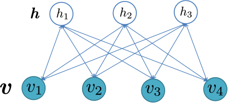
Figure 1: Graphical model of a RBM that models joint distribution of 4 visible units and 3 hidden units. The connections are undirected and the shade nodes are observed.

3.1.1 Model representation

Let $\boldsymbol{v}$ denote the set of visible variables: $\boldsymbol{v}=\left\{v_{1},v_{2},...,v_{N}\right\}$, $\boldsymbol{h}$ indicate the set of hidden ones: $\boldsymbol{h}=\left\{h_{1},h_{2},...,h_{K}\right\}$. RBM assigns probabilities to variables basing on energy theory [32]. Thus, RBM is a energy-based model which captures dependencies between variables by attaching a scalar energy, a measure of compatibility, to each configuration of the variables. The learning phase of energy-based model seeks an energy function that minimises energies of correct values and maximises for incorrect values [41]. In RBM case, energy function of a joint configuration $\left(\boldsymbol{v},\boldsymbol{h}\right)$ is given by

$$E\left(\boldsymbol{v},\boldsymbol{h};\psi\right)=-\boldsymbol{a}^{\top}\boldsymbol{v}-\boldsymbol{b}^{\top}\boldsymbol{h}-\boldsymbol{h}^{\top}\boldsymbol{W}\boldsymbol{v}$$

where $\psi=\left\{\boldsymbol{a}\mathbf{,}\boldsymbol{b},\boldsymbol{W}\right\}$ is the set of parameters with $\boldsymbol{a},\boldsymbol{b}$ are biases of hidden and visible units, respectively, and $\boldsymbol{W}$ represents the weights connecting hidden and visible units. The network assigns a probability to every pairwise configuration

$$P\left(\boldsymbol{v},\boldsymbol{h};\psi\right)=\frac{1}{\mathcal{Z}\left(\psi\right)}e^{-E\left(\boldsymbol{v},\boldsymbol{h};\psi\right)}$$ (1)

Note that $\mathcal{Z}\left(\psi\right)$ express the partition function or normalise factor, given by summing over all possible configuration pairs of visible and hidden units

$$\mathcal{Z}\left(\psi\right)=\sum_{\boldsymbol{v},\boldsymbol{h}}e^{-E\left(\boldsymbol{v},\boldsymbol{h};\psi\right)}$$ (2)

Marginalizing out $\boldsymbol{h}$, we have the probability that model assigns to visible configuration $\boldsymbol{v}$

$$P\left(\boldsymbol{v};\psi\right)=\sum_{\boldsymbol{h}}P\left(\boldsymbol{v},\boldsymbol{h};\psi\right)=\frac{1}{\mathcal{Z}\left(\psi\right)}\sum_{\boldsymbol{h}}e^{-E\left(\boldsymbol{v},\boldsymbol{h};\psi\right)}$$

Interestingly, RBM itself possesses a striking property of dependence among variables. Since RBM has no intra-layer connections, every pairs of units in each layer suffer conditional independence on another layer. Hence, the conditional distributions over hidden and visible units are factorised as

$$P\left(\boldsymbol{v}\mid\boldsymbol{h};\psi\right) = \prod_{i=1}^{N}P\left(v_{i}\mid\boldsymbol{h}\right)$$ (3)

$$P\left(\boldsymbol{h}\mid\boldsymbol{v};\psi\right) = \prod_{j=1}^{K}P\left(h_{j}\mid\boldsymbol{v}\right)$$ (4)

3.1.2 Parameter Learning

As mentioned above, the model adjusts parameters $\psi=\left\{\boldsymbol{a},\boldsymbol{b},\boldsymbol{W}\right\}$ to minimise energies as equivalent to maximise the probabilities assigned to data. The data likelihood is marginal distribution of visible configuration $\boldsymbol{v}$: $\mathcal{L}=P\left(\boldsymbol{v};\psi\right)=\sum_{\boldsymbol{h}}P\left(\boldsymbol{v},\boldsymbol{h};\psi\right)$. Parameter estimation might be performed by using gradient ascent to maximise likelihood. Apparently, another description of Eq. (1) is as below

$$P\left(\boldsymbol{v},\boldsymbol{h};\psi\right) = \exp\left\{-E\left(\boldsymbol{v},\boldsymbol{h};\psi\right)-\log\mathcal{Z}\left(\mathbf{\psi}\right)\right\}$$ (5)

$$= \exp\left\{\boldsymbol{a}^{\top}\boldsymbol{v}+\boldsymbol{b}^{\top}\boldsymbol{h}+\boldsymbol{h}^{\top}\boldsymbol{W}\boldsymbol{v}-A\left(\psi\right)\right\}$$

where $A\left(\psi\right)=\log\mathcal{Z}\left(\psi\right)$ is log-partition function. It is clear that Eq. (5) forms an exponential function. Therefore, RBM belongs to exponential family. The gradient of $\log\mathcal{L}$ with respect to parameters holds the type of difference of expectations

$$\frac{\partial}{\partial\psi}\left(\log\mathcal{L}\left(\boldsymbol{v};\psi\right)\right)=\mathbb{E}_{\boldsymbol{v},\boldsymbol{h}}\left[\frac{\partial E\left(\boldsymbol{v},\boldsymbol{h}\right)}{\partial\psi}\right]-\mathbb{E}_{\boldsymbol{h}\mid\boldsymbol{v}}\left[\frac{\partial E\left(\boldsymbol{v},\boldsymbol{h}\right)}{\partial\psi}\right]$$ (6)

$\mathbb{E}_{\boldsymbol{v},\boldsymbol{h}}$ describes the expectation with respect to full model distribution $P\left(\boldsymbol{v},\boldsymbol{h};\psi\right)=P\left(\boldsymbol{h}\mid\boldsymbol{v};\psi\right)P\left(\boldsymbol{v};\psi\right)$. $\mathbb{E}_{\boldsymbol{h}\mid\boldsymbol{v}}$ denotes the expectation with respect to conditional distribution given known $\boldsymbol{v}$. To be more specific, the derivative of the log-likelihood with respect to model parameters can be computed as below

$$\frac{\partial\log\mathcal{L}\left(\boldsymbol{v};\psi\right)}{\partial\boldsymbol{W}} = \mathbb{E}_{P_{\textnormal{data}}}\left[\boldsymbol{h}^{\top}\boldsymbol{v}\right]-\mathbb{E}_{P_{\textnormal{model}}}\left[\boldsymbol{h}^{\top}\boldsymbol{v}\right]$$ (7)

$$\frac{\partial\log\mathcal{L}\left(\boldsymbol{v};\psi\right)}{\partial\boldsymbol{a}} = \mathbb{E}_{P_{\textnormal{data}}}\left[\boldsymbol{v}\right]-\mathbb{E}_{P_{\textnormal{model}}}\left[\boldsymbol{v}\right]$$ (8)

$$\frac{\partial\log\mathcal{L}\left(\boldsymbol{v};\psi\right)}{\partial\boldsymbol{b}} = \mathbb{E}_{P_{\textnormal{data}}}\left[\boldsymbol{h}\right]-\mathbb{E}_{P_{\textnormal{model}}}\left[\boldsymbol{h}\right]$$ (9)

Thanks to the factorisation in Eq. (4), it is simple to compute the data expectation. However, the model expectation is intractable to estimate exactly. Consequently, several approximate methods must be considered. In this report, we choose Markov Chain Monte Carlo (MCMC) method, one of the most powerful samplers. Due to factorisations in Eq. (3,4), MCMC enables us to do sampling and approximate efficiently. More particularly, alternating Gibbs sampling between hidden and visible units, $\hat{\boldsymbol{v}}\sim P\left(\boldsymbol{v}\mid\hat{\boldsymbol{h}}\right)$ and $\hat{\boldsymbol{h}}\sim P\left(\boldsymbol{h}\mid\hat{\boldsymbol{v}}\right)$, supplies samples of the equilibrium distribution. On one hand, all hidden and visible units are updated in parallel in individual iteration of Gibbs sampling. After estimating states for hidden units, the process changes into a reconstruction step in which visible states are computed and then sampled on them. The difference between first step and last reconstruction step shows how much parameters should be changed in order to conduct data distribution closely to equilibrium distribution. On the other hand, the learning is able to be pushed to higher speed by applying Contrastive Divergence (CD) [30], a truncated MCMC-based method, which in fact is Kullback-Liebler divergence of two distributions. In Contrastive Divergence, the Markov Chain is restarted to each observed sample at each stage and then all parameters are updated. $\textnormal{CD}{}_{n}$ denotes using $n$ full steps of alternating Gibbs sampling. In practical experiment, $\textnormal{CD}{}_{1}$ is used more frequently since it is proved that Kullback-Liebler divergence reduces after each step [30]. Especially with large training dataset, $\textnormal{CD}{}_{1}$ is much more faster than $\textnormal{CD}{}_{n}$. It also has low variance, but still provides dramatic difference from equilibrium distribution when the mixing rate is low. An algorithm called Persistent Contrastive Divergence (PCD) was introduced in [77]. Instead of resetting Markov Chain between parameters updates, in PCD, they initialise the chain at the state in which it ended at the previous one. This way of initialisation contributes fairly closer to model distribution, even though the model slightly changes after parameters updates.

Once samples have been supplied, the parameters are updated in a gradient ascent fashion as follows

$$\psi\leftarrow\psi+\lambda\left(\mathbb{E}_{\boldsymbol{v},\boldsymbol{h}}\left[\frac{\partial E\left(\boldsymbol{v},\boldsymbol{h}\right)}{\partial\psi}\right]-\mathbb{E}_{\boldsymbol{h}\mid\boldsymbol{v}}\left[\frac{\partial E\left(\boldsymbol{v},\boldsymbol{h}\right)}{\partial\psi}\right]\right)$$ (10)

for some learning rate $\lambda>0$. Because the expectations in Eq. (10) can be estimated after taking each sample or mini-batch of samples, it is more efficient to use stochastic gradient ascent instead of normal gradient ascent. The algorithm to learn parameters for RBM using $\textnormal{CD}_{1}$ is described as in Alg. 1.

Input:

Sample $\boldsymbol{v}_{0}$, learning rate $\lambda$ as in Eq. (10).

$\left\{\boldsymbol{a},\boldsymbol{b},\boldsymbol{W}\right\}$ is the set of parameters of RBM as in Eq. (5).

 

1:  for  $j=1$ to $K$  do

2:      $P\left(h_{0j}=1\mid\boldsymbol{v}_{0}\right)=\textnormal{sigm}\left(b_{j}+\sum_{i}v_{0i}W_{ij}\right)$

3:      $h_{0j}\sim P\left(h_{0j}=1\mid\boldsymbol{v}_{0}\right)$

4:  end for

5:  for  $i=1$ to $N$  do

6:      $P\left(v_{1i}=1\mid\boldsymbol{h}_{0}\right)=\textnormal{sigm}\left(a_{i}+\sum_{j}h_{0j}W_{ij}\right)$

7:      $v_{1i}\sim P\left(v_{1i}=1\mid\boldsymbol{h}_{0}\right)$

8:  end for

9:  for  $j=1$ to $K$  do

10:      $P\left(h_{1j}=1\mid\boldsymbol{v}_{1}\right)=\textnormal{sigm}\left(b_{j}+\sum_{i}v_{1i}W_{ij}\right)$

11:  end for

12:   $\boldsymbol{W}\leftarrow\boldsymbol{W}+\lambda\left(\boldsymbol{h}_{0}\boldsymbol{v}_{0}^{\top}-P\left(h_{1j}=1\mid\boldsymbol{v}_{1}\right)\boldsymbol{v}_{1}^{\top}\right)$

13:   $\boldsymbol{a}\leftarrow\boldsymbol{a}+\lambda\left(\boldsymbol{v}_{0}-\boldsymbol{v}_{1}\right)$

14:   $\boldsymbol{b}\leftarrow\boldsymbol{b}+\lambda\left(\boldsymbol{h}_{0}-P\left(h_{1j}=1\mid\boldsymbol{v}_{1}\right)\right)$

 

Output: $\left\{\boldsymbol{a},\boldsymbol{b},\boldsymbol{W}\right\}$.

Algorithm 1 Learning parameters of RBM using Contrastive Divergence.

Parameter learning of RBM benefits enormously in deep learning. In this field, RBM is considered as an infinite belief networks with tied weights [28]. A deep belief network (DBN) is a hybrid network with multiple layers. Top two layers contain undirected connections forming an associative memory while the layers below have directed ones. This kind of deep networks might be pretrained layer-by-layer with individual two layers forming a RBM. After initialising weights by using multiple RBMs, all parameters of this hierarchical model are fine-tuned by back-propagation similar to neural networks. The advantages of unsupervised pretraining with respect to deep architectures are proved empirically in [19].

3.1.3 Inference

The aim of learning RBM is to study a generative model that generates visible data, also known as training data. This benefits in numerous applications including dimensionality reduction, feature extraction [29] and data completion as well as collaborative filtering [62]. For the former one, the posterior projection of RBM is useful for feature extraction tool and used as new domain of features with lower dimension. Once the model has been estimated, visible input data can be transformed into real-valued hidden vector $\hat{\boldsymbol{h}}=\left(\hat{h}_{1},\hat{h}_{2},...,\hat{h}_{K}\right)$, where $\hat{h}_{k}=P\left(h_{k}=1\mid\boldsymbol{v}\right)$. It is conspicuous that handling vector in form of $\hat{\boldsymbol{h}}$ are much more convenient than original data vector $\boldsymbol{v}$, especially when the data types are mixed [82] (see Section 3.2). RBM learns data in generative way with whole information in numerous types condensed in numerical hidden posterior vectors. Consequently, these numerical vectors are fed into next data analysis tools to do clustering, classification, prediction, even continue reduce dimension like multilayer encoder network [29]. To present evidence for reserving data information, we reconstruct the original data using $\hat{\boldsymbol{v}}=\left(\hat{v}_{1},\hat{v}_{2},...,\hat{v}_{N}\right)$, where $\hat{v}_{n}\sim P\left(v_{n}\mid\hat{\boldsymbol{h}}\right)$ and then estimate the average error of $\boldsymbol{v}$ and $\hat{\boldsymbol{v}}$. When it comes to the latter one, let $\boldsymbol{v}_{\neg S}$ denote the set of observed variables, and $\boldsymbol{v}_{S}$ depict the set of unseen variables to be fulfilled. It is necessary to compute the inference of $P\left(\boldsymbol{v}_{S}\mid\boldsymbol{v}_{\neg S}\right)$. Since this inference demands an exponential computation if simultaneously calculated, $P\left(v_{i}\mid\boldsymbol{v}_{\neg S}\right)$, $i\in S$, is estimated instead.

3.1.4 Type-specific data of RBM

Recall that RBM is capable of modelling numerous types of data (e.g., binary, Gaussian, categorical, Poisson or count and softmax data). For individual type, there are changes in the model and parameters which causes to difference of energy, probabilities function. We are assumed that hidden units are binary. Nonetheless, applying to variant types of hidden units is absolutely similar to visible ones.

Let $\tau\left(x\right)$ denote the logistic sigmoid function$\tau\left(x\right)=\frac{1}{1+e^{-x}}$. The activation probability of hidden units are specified as $P\left(h_{j}=1\mid\boldsymbol{v}\right)=\tau\left(b_{j}+\sum_{i}v_{i}W_{ij}\right)$. Here we specify formula modifications for almost types of visible units that RBM is able to handle.

• Binary data: $P\left(v_{i}=1\mid\boldsymbol{h}\right)=\tau\left(a_{i}+\sum_{j}h_{j}W_{ij}\right)$.

• Gaussian data: The logistic units have a poor representation for real-valued data such as natural images, Mel-Cepstrum coefficients used to represent speech [47]. These binary visible units can be replaced by linear units with independent Gaussian noise. Let $\sigma_{i}$ denote the standard deviation of the Gaussian noise for visible unit $v_{i}$. The energy function then becomes

  $$E\left(\boldsymbol{v},\boldsymbol{h}\right)=\sum_{i=1}^{N}\frac{\left(v_{i}-a_{i}\right)^{2}}{2\sigma_{i}^{2}}-\sum_{j=1}^{K}b_{j}h_{j}-\sum_{i=1}^{N}\sum_{j=1}^{K}W_{ij}\frac{v_{i}}{\sigma_{i}}h_{j}$$ (11)

  where $\sigma_{i}$ is the standard deviation of the Gaussian noise for visible unit $i$. The visible and hidden probabilities are computed as follows

  $$P\left(v_{i}=n\mid\boldsymbol{h}\right) = \mathcal{N}\left(a_{i}+\sigma_{i}\sum_{j}h_{j}W_{ij};\sigma_{i}^{2}\right)$$

  $$= \frac{1}{\sqrt{2\pi}\sigma_{i}}\exp\left\{-\frac{\left(n-a_{i}-\sigma_{i}\sum_{j}h_{j}W_{ij}\right)^{2}}{2\sigma_{i}^{2}}\right\}$$

  $$P\left(h_{j}=1\mid\boldsymbol{v}\right) = \tau\left(b_{j}+\sum_{i}W_{ij}\frac{v_{i}}{\sigma_{i}}\right)$$

  It is feasible to learn the variance of the noise for each visible unit. However, it is complicated for using CD. To make learning easier, we first normalise each feature of data to have zero mean and unit variance. The standard variance $\sigma$ in Eq. (11) is then set to 1. Then we can use noise-free top-down reconstructions from hidden units to input data. The learning rate $\lambda$ in Eq. (10) must be smaller because there is no upper bound to the value.

• Poisson data: To represent count (e.g., document words, diagnosis codes, bag-of-visual words), we adopt the constrained Poisson model by [60]. Denote the Poisson probability mass function by $Ps\left(n,\mu\right)=e^{-\mu}\frac{\mu^{n}}{n!}$, in which $\mu$ is the mean or bias of the conditional Poisson model. Visible probabilities are given by

  $$P\left(v_{i}=n\mid\boldsymbol{h}\right) = Ps\left(n,\frac{\exp\left(a_{i}+\sum_{j}h_{j}W_{ij}\right)}{\sum_{k}\exp\left(a_{k}+\sum_{j}h_{j}W_{ij}\right)}N\right)$$

  where $N=\sum_{i}v_{i}$ is the length of count data (e.g., document, total number of diagnosis codes).

• Softmax data: Referring to the binary data, the probability of turning on a unit is given by the logistic sigmoid function. Each probability of two possible states, i.e., 1 is on, 0 is off, is proportional to the negative exponential of its energy. We can generalise to $M$ alternative states

  $$P\left(v_{i}^{m}=1\mid\boldsymbol{h}\right)=\frac{\exp\left\{a_{i}^{k}+\sum_{j}h_{j}W_{ij}^{m}\right\}}{\sum_{t}\exp\left\{a_{i}^{t}+\sum_{j}h_{j}W_{ij}^{t}\right\}}$$

  These types of units can be called as “softmax” units. It is suitable for modelling the data that has $M$ unordered options. As can be seen, a softmax can be considered as a set of binary units. Thus each binary unit in a softmax should be learned in the same way as standard binary units. However, the hidden and visible probabilities are computed differently. The hidden probability is now computed as

  $$P\left(h_{j}=1\mid\boldsymbol{v}\right)=\tau\left(b_{j}+\sum_{i}\sum_{m}v_{i}^{m}W_{ij}^{m}\right)$$

  Replicated Softmax:

  When softmax units appear repeatedly in visible vectors, e.g. words in documents, diagnosis codes in history of patients, Salakhutdinov et al. [61] introduced a separate RBM with the number of softmax units be exactly the same as number of units of a visible vector. These visible units can be called as Replicated Softmax units. Assume that the order of units can be ignored, entire softmax units can share the same set of weights as well as parameters which connects them to hidden units. Let $\boldsymbol{v}\in\left\{q_{1},q_{2},..,q_{N}\right\}^{D}$, in which $N$ is total number of distinguished values that can be assigned to one unit, $D$ is the actual number of units in a data vector. Denote $K$ be the number of binary hidden units. Replicated Softmax RBM models the appearance of visible softmax unit with $v_{i}^{n}=1$ if visible unit takes on $q_{n}$. Consider $\hat{v}_{i}=\sum_{d=1}^{D}v_{d}^{i}$ as the count for value $q_{i}$. The energy function is given as below

  $$E\left(\boldsymbol{v},\boldsymbol{h}\right)=-\sum_{i=1}^{N}a_{i}\hat{v}_{i}-D\sum_{j=1}^{K}b_{j}h_{j}-\sum_{i=1}^{N}\sum_{j=1}^{K}W_{ij}\hat{v}_{i}h_{j}$$ (12)

  As the same as softmax units, we have the visible and hidden probabilities

  $$P\left(v_{i}^{n}=1\mid\boldsymbol{h}\right) = \frac{\exp\left\{a_{n}+\sum_{j=1}^{K}h_{j}W_{nj}\right\}}{\sum_{t=1}^{N}\exp\left\{a_{t}+\sum_{j=1}^{K}h_{j}W_{tj}\right\}}$$ (13)

  $$P\left(h_{j}=1\mid\hat{\boldsymbol{v}}\right) = \tau\left(Db_{j}+\sum_{i=1}^{N}W_{ij}\hat{v}_{i}\right)$$ (14)

• Categorical data: Let $M$ describe the number of categories. Denote by $S=\left\{c_{1},c_{2},...,c_{M}\right\}$ the set of categories. Let $\pi\left[v_{i}\right]$ be a $M$-dimension vector with $\pi_{m}\left[v_{i}\right]=1$ if $v_{i}=c_{m}$ and 0 otherwise. Here are the following energy, visible and hidden probabilities functions

  $$E\left(\boldsymbol{v},\boldsymbol{h}\right) = -\sum_{i=1}^{N}\sum_{m=1}^{M}a_{i}^{m}\pi_{m}\left[v_{i}\right]-\sum_{j=1}^{K}b_{j}h_{j}-\sum_{i=1}^{N}\sum_{m=1}^{M}\sum_{j=1}^{K}W_{ij}^{m}\pi_{m}\left[v_{i}\right]h_{j}$$

  $$P\left(v_{i}^{m}=1\mid\boldsymbol{h}\right) = \frac{\exp\left\{\sum_{m=1}^{M}a_{i}^{m}\pi_{m}\left[v_{i}\right]+\sum_{m=1}^{M}\sum_{j=1}^{K}W_{ij}^{m}\pi_{m}\left[v_{i}\right]h_{j}\right\}}{\sum_{l=1}^{M}\exp\left\{a_{i}^{l}+\sum_{j=1}^{K}W_{ij}^{l}h_{j}\right\}}$$

  $$P\left(h_{j}=1\mid\boldsymbol{v}\right) = \tau\left(b_{j}+\sum_{i=1}^{N}\sum_{m=1}^{M}W_{ij}^{m}\pi_{m}\left[v_{i}\right]\right)$$

3.2 Mixed-Variate Restricted Boltzmann Machine

3.2.1 Model representation

Mixed-Variate Restricted Boltzmann Machine (MV.RBM) is introduced by Truyen et al. [82]. A Mixed-Variate RBM is a RBM with heterogeneous input units, each of which has the own type. See, for example, Figure 2 in Section 4.1.1 for an illustration. More formally, let $\boldsymbol{v}$ denote the joint set of visible variables: $\boldsymbol{v}=\left(v_{1},v_{2},...,v_{N}\right)$, $\boldsymbol{h}$ the joint set of binary hidden units: $\boldsymbol{h}=\left(h_{1},h_{2},...,h_{K}\right)$, where $h_{k}\in\left\{0,1\right\}$ for all $k$. Each visible unit encodes type-specific information, and the hidden units capture the latent factors not presented in the observations. Thus the MV.RBM can be seen as a way to transform inhomogeneous observational record into a homogeneous representation of the patient profile. Another way to view this as a mixture model where there are $2^{K}$ mixture components. This capacity is arguably important to capture all factors of variation in the patient cohort.

The MV.RBM defines a Boltzmann distribution over all variables: $P\left(\boldsymbol{v},\boldsymbol{h};\psi\right)=e^{-E\left(\boldsymbol{v},\boldsymbol{h}\right)}/Z\left(\psi\right)$, where $E\left(\boldsymbol{v},\boldsymbol{h}\right)$ is model energy, $Z\left(\psi\right)$ is the normalising constant and $\psi$ is model parameter. In particular, the energy is defined as

$$E\left(\boldsymbol{v},\boldsymbol{h};\psi\right)=-\left(\sum_{i}F(v_{i})+\boldsymbol{a}^{\top}\boldsymbol{v}+\boldsymbol{b}^{\top}\boldsymbol{h}+\boldsymbol{h}^{\top}\boldsymbol{W}\boldsymbol{v}\right)$$ (15)

where $F(v_{i})$ is the type-specific function, $\boldsymbol{a}=\left(a_{1},a_{2},...,a_{N}\right)$ and $\boldsymbol{b}=\left(b_{1},b_{2},...,b_{K}\right)$ are biases of visible and hidden units respectively, and $\boldsymbol{W}=\left[W_{ij}\right]$ are the weights connecting hidden and visible units. Because the visible variables of MV.RBM is mixed-variate, $\boldsymbol{v}$ consists of $\left(\boldsymbol{v}_{disc},\boldsymbol{v}_{cont}\right)$, where $\boldsymbol{v}_{disc}$ defines the joint set of discrete variables and $\boldsymbol{v}_{cont}$ is the joint set of continuous ones. The integration must be involved into the partition function in Eq. (2), which is given by

$$\mathcal{Z}\left(\psi\right)=\int_{\boldsymbol{v}_{cont}}\left(\sum_{\boldsymbol{v}_{dist},\boldsymbol{h}}\exp\left\{-E\left(\boldsymbol{v}_{dist},\boldsymbol{v}_{cont},\boldsymbol{h};\psi\right)\right\}\right)d\left(\boldsymbol{v}_{cont}\right)$$

Similarity to plain RBM, the MV.RBM comprises conditional independence among intra-layer variables which lead to hidden and visible factorisations in Eqs. (3,4). The type-specific function $F(v_{i})$ can be pointed out for individual type basing on its probabilistic function in Section 3.1.4. For example, For example, let $f_{i}(\boldsymbol{h})=a_{i}+\sum_{k}W_{ik}h_{k}$, the binary units would be specified as: $P\left(v_{i}\mid\boldsymbol{h}\right)=1/\left(1+e^{-f_{i}(\boldsymbol{h})}\right)$ (i.e., $F_{i}(v_{i})=0$); the Gaussian units: $P\left(v_{i}\mid\boldsymbol{h}\right)=\mathcal{N}\left(\sigma_{i}^{2}f_{i}(\boldsymbol{h});\sigma_{i}\right)$ (i.e., $F_{i}(v_{i})=-v_{i}^{2}/2\sigma_{i}^{2}$), and the categorical units: $P\left(v_{i}\mid\boldsymbol{h}\right)=e^{f_{i}(\boldsymbol{h})}/\sum_{j}e^{f_{j}(\boldsymbol{h})}$.

3.2.2 Extensions

The Poisson and “replicated softmax” are not readily available in the current MV.RBM of Truyen et al. [82]. In this work, we attempt to introduce these two types to the machine. To be easier, we consider visible units represent words in a document for an instance. The other count data (e.g., bag-of-visual words, diagnosis codes of a patient) are equivalent. To represent counts, we adopt the constrained Poisson model by [60] in that $P\left(v_{i}=n\mid\boldsymbol{h}\right)=\mbox{Poisson}\left(n,\frac{\exp\left\{f_{i}(\boldsymbol{h})\right\}}{\sum_{k}\exp\left\{f_{i}(\boldsymbol{h})\right\}}L\right)$, where $L$ is the “document” length. With “replicated softmax”, we adopt the idea from [61] where repeated words share the same parameters. In the end, we build one MV.RBM per document due to the difference in the word sets. Further, to balance the contribution of the hidden units against the variation in input length, it is important to make a change to the energy model in Eq. (15) as follows: $D\boldsymbol{b}\leftarrow\boldsymbol{b}$ where $D$ is the total number of input variables for each document. We show the efficiency of these parameter sharing and balancing in Section 4.

3.2.3 Parameters learning and Inference

Because the gradient of log-likelihood still forms model and data expectations as in Eq. (6), Contrastive Divergence (CD) obviously can be used to approximate model expectation. Then we apply gradient ascent manner as in Eq. (10) to learn parameters of MV.RBM.

In [82], Truyen et al. also show that the MV.RBM is capable to construct a predictive model and then do prediction on unseen variables given observed ones. Let $\boldsymbol{v}_{S}$ depict the set of unseen variables to be fulfilled,$\boldsymbol{v}_{\neg S}$ denote the set of observed variables. The problem is of estimating the conditional distribution $P\left(\boldsymbol{v}_{S}\mid\boldsymbol{v}_{\neg S}\right)$. Assuming that unseen variables are pair-wise independent, $P\left(v_{i}\mid\boldsymbol{v}_{\neg S}\right)$, $i\in S$, is estimated instead. There are two common ways: generative and discriminative methods to learn a predictive model. The former attempts to model the joint distribution $P\left(v_{i},\boldsymbol{v}_{\neg S}\right)$. The learning is now of maximising the following likelihood

$$\mathcal{L}_{1}=\sum_{\boldsymbol{v}_{\neg S}}\tilde{P}\left(\boldsymbol{v}_{\neg S}\right)\log P\left(\boldsymbol{v}_{\neg S}\right)$$ (16)

The latter one is to directly model the conditional distribution $P\left(v_{i}\mid\boldsymbol{v}_{\neg S}\right)$ which is equivalent to maximise the conditional likelihood given as below

$$\mathcal{L}_{2}=\sum_{v_{i}}\sum_{\boldsymbol{v}_{\neg S}}\tilde{P}\left(v_{i},\boldsymbol{v}_{\neg S}\right)\log P\left(v_{i}\mid\boldsymbol{v}_{\neg S}\right)$$ (17)

It can be seen that the discriminative method requires less computational complexity since we do not have to estimate $P\left(\boldsymbol{v}_{\neg S}\right)$. But the capability of MV.RBM is to unsupervised learn joint distribution and then do projections $P\left(\boldsymbol{h}\mid\boldsymbol{v}_{\neg S}\right)$, in the work of Truyen et al., they follow the third approach. It is a hybrid method that linear combine generative and discriminative methods as follows

$$\mathcal{L}_{3} = \lambda\mathcal{L}_{1}+\left(1-\lambda\right)\mathcal{L}_{2}$$

$$= \lambda\sum_{\boldsymbol{v}_{\neg S}}\tilde{P}\left(\boldsymbol{v}_{\neg S}\right)\log P\left(\boldsymbol{v}_{\neg S}\right)+\left(1-\lambda\right)\sum_{v_{i}}\sum_{\boldsymbol{v}_{\neg S}}\tilde{P}\left(v_{i},\boldsymbol{v}_{\neg S}\right)\log P\left(v_{i}\mid\boldsymbol{v}_{\neg S}\right)$$

where $\lambda\in\left(0,1\right)$ is the coefficient to adjust the effect of two methods on the final likelihood. There are two ways to maximise the likelihood $\mathcal{L}_{3}$. One optimises both likelihood $\mathcal{L}_{1}$ and $\mathcal{L}_{2}$ simultaneously. Another is to use 2-stage procedure: first pretrain $P\left(\boldsymbol{v}_{\neg S}\right)$ using unsupervised fashion and then fine-tune the predictive model $P\left(v_{i}\mid\boldsymbol{v}_{\neg S}\right)$ by discriminative training.

3.3 Integrating Structured Sparsity

Recall that hidden posteriors which are projected using RBM or MV.RBM form latent representations. These latent representations capture the regularities of the data. Nonetheless, they are not readily unstructured and disentangle all the factors of variation. Since, for example, the image frequently describes a few types of objects, the probabilistic activations of hidden units should be controlled for better representation. One way to do improve representation is to incorporate structured sparsity which supports better separation of object groups and easier interpretation. Following the previous work [44], we apply mixed-norm $\nicefrac{{l_{1}}}{{l_{2}}}$ regulariser on the latent representation. Hidden units in latent representation are also equally arranged into non-overlapped groups. The mixed-norm regulariser can control both inter-group and intra-group hidden activations.

Denote $\mathcal{H}$ by the set of all hidden units indices: $\mathcal{H}=\left\{1,2,...,K\right\}$. We divide hidden units into $M$ non-overlapped groups with equal sizes. Let $\mathcal{G}_{m}$ describe the indices of hidden units in group $m^{th}$, where $G_{m}\subset\mathcal{H}$. $l_{2}\textnormal{-norm}$ of the $m^{th}$ group is given by

$$\mathcal{R}{}_{2}^{\left(m\right)}\left(\boldsymbol{v}\right)=\sqrt{\sum_{j\in G_{m}}P\left(h_{j}=1\mid\boldsymbol{v}\right)^{2}}$$ (18)

From that, the mixed-norm $\nicefrac{{l_{1}}}{{l_{2}}}$ is defined as $l_{1}\textnormal{-norm}$ regularising over all $M$ groups as follows

$$\mathcal{R}\left(\boldsymbol{v}\right)=\sum_{m=1}^{M}\left|\mathcal{R}_{2}^{\left(m\right)}\left(\boldsymbol{v}\right)\right|=\sum_{m=1}^{M}\sqrt{\sum_{j\in G_{m}}P\left(h_{j}=1\mid\boldsymbol{v}\right)^{2}}$$ (19)

The way to integrate structured sparsity is to involve the regulariser into the log-likelihood of RBM. The learning of RBM then operates both updating parameters and enhancing the structured sparsity of latent representations simultaneously. The integration defines a new likelihood function of RBM as below

$$\mathcal{L}_{spr}\left(\boldsymbol{v};\psi\right)=\log\mathcal{L}\left(\boldsymbol{v};\psi\right)-\alpha\mathcal{R}\left(\boldsymbol{v}\right)$$ (20)

where $\alpha\geq 0$ is the regularising constant for sparsity. Basing on the gradient of log-likelihood function in Eq. (6), we obtain the following gradient of the likelihood

$$\frac{\partial}{\partial\psi}\mathcal{L}_{spr}\left(\boldsymbol{v};\psi\right)=\mathbb{E}_{\boldsymbol{v},\boldsymbol{h}}\left[\frac{\partial E\left(\boldsymbol{v},\boldsymbol{h}\right)}{\partial\psi}\right]-\mathbb{E}_{\boldsymbol{h}\mid\boldsymbol{v}}\left[\frac{\partial E\left(\boldsymbol{v},\boldsymbol{h}\right)}{\partial\psi}\right]-\alpha\frac{\partial}{\partial\psi}\mathcal{R}\left(\boldsymbol{v}\right)$$ (21)

The derivatives of first two expectations in Eq. (21) with respect to model parameters can be estimated using Eqs. (7,8,9). Here we specify the added regularisation $\mathcal{R}\left(\boldsymbol{v}\right)$. Note that $\left|\mathcal{R}_{m}\left(\boldsymbol{v}\right)\right|=\mathcal{R}_{m}\left(\boldsymbol{v}\right)$ since $\mathcal{R}_{m}\left(\boldsymbol{v}\right)\geq 0$. Thus, we have these following deductions

$$\mathcal{R}\left(\boldsymbol{v}\right) = \sum_{m=1}^{M}\mathcal{R}_{m}\left(\boldsymbol{v}\right)$$

$$= \sum_{m=1}^{M}\sqrt{\sum_{t\in\mathcal{G}_{m}}P\left(h_{t}=1\mid\boldsymbol{v}\right)^{2}}$$

$$= \sqrt{\sum_{t\in\mathcal{G}_{\hat{m}}}P\left(h_{t}=1\mid\boldsymbol{v}\right)^{2}}$$

$$= \sqrt{\sum_{t\in\mathcal{G}_{\hat{m}},t\neq j}P\left(h_{t}=1\mid\boldsymbol{v}\right)^{2}+P\left(h_{j}=1\mid\boldsymbol{v}\right)^{2}}$$

Taking the derivative of the regularisation with respect to inter-layer parameter $W_{ij}$ and the hidden bias $b_{j}$, it reads

$$\frac{\partial}{\partial b_{j}}\mathcal{R}\left(\boldsymbol{v}\right) = \frac{P\left(h_{j}=1\mid\boldsymbol{v}\right)}{\sqrt{\sum_{t\in\mathcal{G}_{\hat{m}}}P\left(h_{t}=1\mid\boldsymbol{v}\right)^{2}}}\frac{\partial}{\partial b_{j}}P\left(h_{j}=1\mid\boldsymbol{v}\right)$$

$$= \frac{P\left(h_{j}=1\mid\boldsymbol{v}\right)^{2}P\left(h_{j}=0\mid\boldsymbol{v}\right)}{\sqrt{\sum_{t\in\mathcal{G}_{\hat{m}}}P\left(h_{t}=1\mid\boldsymbol{v}\right)^{2}}}$$

$$\frac{\partial}{\partial W_{ij}}\mathcal{R}\left(\boldsymbol{v}\right) = \frac{\partial}{\partial b_{j}}\mathcal{R}\left(\boldsymbol{v}\right)v_{i}$$

During maximising the likelihood, this regulariser is minimised and this leads to group-wise sparsity, i.e., only few groups of hidden units will be activated (e.g., refer to the last column of Figure 8 in Section 4.2). The parameters are updated using stochastic gradient ascent fashion as follows

$$\psi\leftarrow\psi+\lambda\left(\frac{\partial}{\partial\psi}\mathcal{L}_{spr}\right)$$

for some learning rate $\alpha>0$.

3.4 Learning Distance Metric

Latent representation may not fully capture intra/inter-concept variations, and thus it may not result in a good distance metric for retrieval tasks, e.g., image retrieval. It is better to directly learn a distance metric that suppresses intra-concept variation and enlarges inter-concept variation. Given the probabilistic nature of our representation, a suitable distance is the symmetric Kullback-Leibler divergence, also known as Jensen-Shannon divergence:

$$\mathcal{D}\left(g,f\right) = \frac{1}{2}\left(\textnormal{KL}\left(g\|f\right)+\textnormal{KL}\left(f\|g\right)\right)$$ (22)

where $\textnormal{KL}\left(g\|f\right)=\sum_{\boldsymbol{h}}P\left(\boldsymbol{h}\mid g\right)\log\frac{P\left(\boldsymbol{h}\mid g\right)}{P\left(\boldsymbol{h}\mid f\right)}$. Let $\mathsf{N}\left(f\right)$ denote the set of other objects that share the same concept with the object $f$, and $\bar{\mathsf{N}}\left(f\right)$ denotes those do not. The mean distance to all other objects in $\mathsf{N}\left(f\right)$ should be minimised

$$\mathcal{D}_{\mathsf{N}\left(f\right)}=\frac{1}{\left|\mathsf{N}\left(f\right)\right|}\sum_{g\in\mathsf{N}\left(f\right)}\mathcal{D}\left(P\left(\boldsymbol{h}\mid\boldsymbol{v}^{\left(g\right)}\right),P\left(\boldsymbol{h}\mid\boldsymbol{v}^{\left(f\right)}\right)\right)$$ (23)

On the other hand, the mean distance to all images in $\bar{\mathsf{N}}\left(f\right)$ should be enlarged

$$\mathcal{D}_{\bar{\mathsf{N}}\left(f\right)}=\frac{1}{\left|\bar{\mathsf{N}}\left(f\right)\right|}\sum_{g\in\bar{\mathsf{N}}\left(f\right)}\mathcal{D}\left(P\left(\boldsymbol{h}\mid\boldsymbol{v}^{\left(g\right)}\right),P\left(\boldsymbol{h}\mid\boldsymbol{v}^{\left(f\right)}\right)\right)$$ (24)

The idea of intra-concept distance has been studied in [80]. We here enhance the effect of distance metric on learning latent representation with the inter-concept distance. The log-likehood transforms into the new likelihood as follows

$$\mathcal{L}_{ml}=\sum_{f}\log\mathcal{L}\left(\boldsymbol{v}^{\left(f\right)};\psi\right)-\beta\left(\sum_{f}\mathcal{D}_{\mathsf{N}\left(f\right)}-\sum_{f}\mathcal{D}_{\bar{\mathsf{N}}\left(f\right)}\right)$$

where $\beta\geq 0$ is the coefficient to control the effect of distance metrics. Maximising this likelihood is now equivalent to simultaneously maximising the data likelihood $\mathcal{L}\left(\boldsymbol{v};\psi\right)$, minimising the neighbourhood distance $\mathcal{D}_{\mathsf{N}\left(f\right)}$ and maximising the non-neighbourhood distance $\mathcal{D}_{\bar{\mathsf{N}}\left(f\right)}$. From Eq. (6), the gradient of the new likelihood can be given by

$$\frac{\partial}{\partial\psi}\mathcal{L}_{ml}\left(\boldsymbol{v};\psi\right)=\mathbb{E}_{\boldsymbol{v},\boldsymbol{h}}\left[\frac{\partial E\left(\boldsymbol{v},\boldsymbol{h}\right)}{\partial\psi}\right]-\mathbb{E}_{\boldsymbol{h}\mid\boldsymbol{v}}\left[\frac{\partial E\left(\boldsymbol{v},\boldsymbol{h}\right)}{\partial\psi}\right]-\beta\frac{\partial}{\partial\psi}\left(\sum_{f}\mathcal{D}_{\mathsf{N}\left(f\right)}-\sum_{f}\mathcal{D}_{\bar{\mathsf{N}}\left(f\right)}\right)$$ (25)

In Eqs. (7,8,9) above, we already can estimate the derivatives of two expectations. To compute the gradient of the mean distances $\mathcal{D}_{\mathsf{N}\left(f\right)}$ and $\mathcal{D}_{\bar{\mathsf{N}}\left(f\right)}$ defined in Eqs.(23,24), we need the gradient for each pairwise distance $\mathcal{D}\left(g,f\right)=\mathcal{D}\left(P\left(\boldsymbol{h}\mid\boldsymbol{v}^{\left(g\right)}\right),P\left(\boldsymbol{h}\mid\boldsymbol{v}^{\left(f\right)}\right)\right)$. Taking derivative of the metric distance function with respect to parameter $\psi_{\bullet j}$, we have

$$\frac{\partial\mathcal{D}\left(g,f\right)}{\partial\psi_{\bullet j}}=\frac{\partial\mathcal{D}\left(g,f\right)}{\partial P\left(h_{j}^{1}\mid f\right)}\frac{\partial P\left(h_{j}^{1}\mid f\right)}{\partial\psi_{\bullet j}}+\frac{\partial\mathcal{D}\left(g,f\right)}{\partial P\left(h_{j}^{1}\mid g\right)}\frac{\partial P\left(h_{j}^{1}\mid g\right)}{\partial\psi_{\bullet j}}$$ (26)

in which $P\left(h_{j}^{1}\mid f\right)$ is the shorthand for $P\left(h_{j}=1\mid\boldsymbol{v}^{\left(f\right)}\right)$, $\psi_{\bullet j}$ is the parameter associated with hidden units $h_{j}$. Hidden units are assumed to be binary units. Recall from Section 3.1.4 that the probabilistic activations of hidden units are sigmoid functions. Thus the partial derivatives with respect to the mapping column $W_{\bullet j}$ and bias $b_{j}$ are then

$$\frac{\partial P\left(h_{j}^{1}\mid f\right)}{\partial W_{\bullet j}} = P\left(h_{j}^{1}\mid f\right)\left(1-P\left(h_{j}^{1}\mid f\right)\right)\boldsymbol{v}^{\left(f\right)}$$ (27)

$$\frac{\partial P\left(h_{j}^{1}\mid f\right)}{\partial b_{j}} = P\left(h_{j}^{1}\mid f\right)\left(1-P\left(h_{j}^{1}\mid f\right)\right)$$ (28)

As defined in Eq. (22), the derivatives $\frac{\partial\mathcal{D}\left(g,f\right)}{\partial P\left(h_{j}^{1}\mid f\right)}$ and $\frac{\partial\mathcal{D}\left(g,f\right)}{\partial P\left(h_{j}^{1}\mid g\right)}$ depend on the derivative of the KL-divergence, which reads

$$\frac{\partial\textnormal{KL}\left(g\|f\right)}{\partial P\left(h_{j}^{1}\mid g\right)} = \sum_{j}\left(\log\frac{P\left(h_{j}^{1}\mid g\right)}{P\left(h_{j}^{1}\mid f\right)}-\log\frac{1-P\left(h_{j}^{1}\mid g\right)}{1-P\left(h_{j}^{1}\mid f\right)}\right)$$ (29)

$$\frac{\partial\textnormal{KL}\left(f\|g\right)}{\partial P\left(h_{j}^{1}\mid g\right)} = \sum_{j}\left(-\frac{P\left(h_{j}^{1}\mid f\right)}{P\left(h_{j}^{1}\mid g\right)}+\frac{1-P\left(h_{j}^{1}\mid f\right)}{1-P\left(h_{j}^{1}\mid g\right)}\right)$$ (30)

Equivalently to Eqs. (29,30), $\frac{\partial\textnormal{KL}\left(g\|f\right)}{\partial P\left(h_{j}^{1}\mid f\right)}$ and $\frac{\partial\textnormal{KL}\left(f\|g\right)}{\partial P\left(h_{j}^{1}\mid f\right)}$ can be easily computed. Combining all things in Eqs. (27,28,29,30), we can calculate the derivative of the metric distance with respect to parameter $\psi_{\bullet j}$ in Eq. (26).

Finally, the parameters are updated using stochastic gradient ascent fashion as follows

$$\psi\leftarrow\psi+\lambda\left(\frac{\partial}{\partial\psi}\mathcal{L}_{ml}\right)$$

for some learning rate $\alpha>0$.

4 Applications

In this section, we demonstrate the performances of our proposed models in various applications including latent patient profile modelling in medical data analysis (published in [52]) and representation learning for image retrieval (published in [53]). The former application is to implement an extension of Mixed-Variate Restricted Boltzmann Machine (MV.RBM) for clustering patients and predicting diagnosis codes $1$-year in advance. The latter one learns sparse latent representation and distance metric for image retrieval. The experimental results demonstrate the former model gains better results than baseline methods and the latter outperforms state-of-the-art rivals on NUS-WIDE datasets [10].

4.1 Medical data analysis

It is undeniable that health is the most significant factor of human being. Unfortunately, the modern world has been seeing more and more emerging incurable diseases. They adversely impact human life quality as well as consume a huge amount of healthcare expenditures [5]. Besides, chronic illness often extends over many years along with acute exacerbations, progressive deterioration and complications. For example, Diabetes Mellitus is one such chronic disease from which $346$ million people worldwide suffer, as estimated by The World Health Organization (WHO) [56]. Only about $5-10$% of them have Type I diabetes mellitus, whilst Type II comprises the rest. The people who suffer Type I are not able to produce insulin. In contrast, Type II diabetes means that there is an inability to absorb insulin. In 2004, $3.4$ million people died from complications of high blood sugar. The incidence of diabetes mellitus is increasing, and being diagnosed in younger people. This leads to serious complications associated with long disease duration - deterioration in blood vessels, eyes, kidneys and nerves. It is a chronic, lifelong disease.

Consequently, healthcare management requires a scaled-up investigation to improve chronic illness treatment and minimise the exacerbations, slow or halt deterioration, and decrease the cost of care. To provide high quality healthcare, care plans are issued to patients to manage them within the community, taking steps in advance so that these people are not hospitalised. For instance, identifying groups of patients with similar characteristics help them be covered by a coherent care plan. Additionally, if the hospital can predict the disease codes arising from escalating complication of chronic disease, it can adjust financial and manpower resources. Thus useful prediction of codes for chronic disease can lead to service efficiency. Thanks to recent high-tech equipment and information technology applied in healthcare organisations, the quantity of electronic hospital records are substantially increasing. Effective patterns and latent structures discovery from this data can improve healthcare system and optimise the pathology treatment for patients. It does require a rigorous analysis on the data.

Clustering is a natural selection for this task. However, medical data is complex – it is mixed-type containing Boolean data (e.g., male/female), continuous quantities (e.g., age), single categories (e.g., regions), and repeated categories (e.g., disease codes). Traditional clustering methods cannot naturally integrate such data and we choose the extension (see Section 3.2.2) of the MV.RBM [82]. The Mixed-Variate RBM uncovers latent profile factors, enabling subsequent clustering. Using a cohort of $6,931$ chronic diabetes patients with data from 2007 to 2011, we collect $3,178$ diagnosis codes (treated as repeated categories) and combine it with region-of-birth (as categories) and age (as Gaussian variables) to form our dataset. We show clustering results obtained from running affinity propagation (AP) [22], containing 10 clusters and qualitatively evaluate the disease codes of groups. We demonstrate that the Mixed-Variate RBM followed by AP outperforms all baseline methods – Bayesian mixture model and affinity propagation on the original diagnosis codes, and $k$-means and AP on latent profiles, discovered by just the plain RBM [61]. Predicting disease codes for future years enables hospitals to prepare finance, equipment and logistics for individual requirements of patients. Thus prediction of disease codes forms the next part of our study. Using the Mixed-Variate RBM and the dataset described above, we demonstrate that our method outperforms other methods, establishing the versatility of the latent profile discovery with MV.RBM.

The next section presents our patient profile modelling framework. Then, we describe our implementation on the diabetes cohort and demonstrate efficiencies of our methods.

4.1.1 Latent Patient Profiling

A patient profile in modern hospitals typically consists of multiple records including demographics, admissions, diagnoses, surgeries, pathologies and medication. Each record contains several fields, each of which is type-specific. For example, age can be considered as a continuous quantity but a diagnosis code is a discrete element. At the first approximation, each patient can be represented by using a long vector of mixed types. However, joint modelling of mixed types is known to be highly challenging even for a small set of variables [45, 18]. Complete patient profiling, on the other hand, requires handling of thousands of variables. Of equal importance is that the profiling should readily support a variety of clinical analysis tasks such as patient clustering, visualisation and disease prediction. In what follows, we develop a representational and computational scheme to capture such heterogeneity in an efficient way.

The goal of patient profiling is to construct an effective personal representation from multiple hospital records. Here we focus mainly on patient demographics (e.g., age, gender and region-of-birth) and their existing health conditions (e.g., existing diagnoses). For simplicity, we consider a binary gender (male/female). Further, age can be considered as a continuous quantity and thus a Gaussian unit can be used; and region-of-birth and diagnosis as categorical variables. However, since the same diagnosis can be repeated during the course of readmissions, it is better to include them all. In particular, we use the extension of MV.RBM with repeated diagnoses considered as “replicated softmax” units (see Section 3.2.2). See Figure 2 for the illustration of MV.RBM for patient profiling.

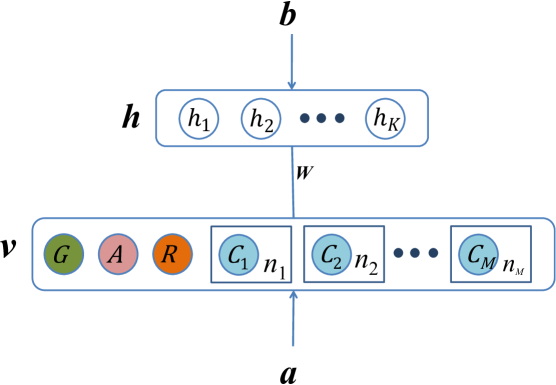
Figure 2: Patient profiling using Mixed-Variate RBMs. The top layer represents stochastic binary units. The bottom layer encodes multiple type-specific inputs: A for age (continuous), G for gender (binary), R for region-of-birth, $C_{k}$ for diagnosis codes. The circles within squares denote the replicated diagnosis codes (categorical) where the integers $\{n_{k}\}$ denotes the number of replications.

Once the model has been estimated, the latent profiles are generated by computing the posterior vector $\hat{\boldsymbol{h}}=\left(P\left(h_{1}^{1}\mid\boldsymbol{v}\right),P\left(h_{2}^{1}\mid\boldsymbol{v}\right),...,P\left(h_{K}^{1}\mid\boldsymbol{v}\right)\right)$, where $P\left(h_{k}^{1}\mid\boldsymbol{v}\right)$is a shorthand for $P\left(h_{k}=1\mid\boldsymbol{v}\right)$ – the probability that the $k$-th latent factor is activated given the demographic and clinical input $\boldsymbol{v}$:

$$P\left(h_{k}^{1}\mid\boldsymbol{v}\right)=\frac{1}{1+\exp\left\{-Db_{k}-\sum_{i}W_{ik}v_{i}\right\}}$$

where $D$ is the total number of input variables for each patient. As we will then demonstrate in Section 4.1.2, the latent profile can be used as input for a variety of analysis tasks such as patient clustering and visualisation.

Interestingly, the model also enables a certain degree of disease prediction, i.e., we want to guess which diagnoses will be positive for the patient in the future. Although this may appear to be an impossible task, it is plausible statistically because some diseases are highly correlated or even causative, and there are certain pathways that a disease may progress. More specifically, subset of diagnoses at time $t+1$ can be predicted by searching for the mode of the following conditional distribution:

$$P\left(\boldsymbol{v}^{(t+1)}\mid\boldsymbol{v}^{(1:t)}\right)=\sum_{\boldsymbol{h}}P\left(\boldsymbol{v}^{(t+1)},\boldsymbol{h}\mid\boldsymbol{v}^{(1:t)}\right)$$

Unfortunately the search is intractable as we need to traverse through the space of all possible disease combinations, which has the size of $2^{M}$ where $M$ is the set of diagnosis codes. To simplify the task and to reuse of the readily discovered latent profile $\hat{\boldsymbol{h}}^{(1:t)}$, we assume that (i) the model distribution is not changed due to the “unseen” future, (ii) the latent profile at this point captures everything we can say about the state of the patient, and (iii) future diseases are conditionally independent given the current latent profile. This leads to the following mean-field approximation:

$$P\left(v_{j}^{(t+1)}\mid\boldsymbol{v}^{(1:t)}\right)\approx\frac{\exp\left\{a_{j}+\sum_{k}W_{jk}P\left(h_{k}^{1}\mid\boldsymbol{v}^{(1:t)}\right)\right\}}{\sum_{i}\exp\left\{a_{i}+\sum_{k}W_{ik}P\left(h_{k}^{1}\mid\boldsymbol{v}^{(1:t)}\right)\right\}}$$ (31)

4.1.2 Implementation and Results

Here we present the analysis of patient profiles using the data obtained from Barwon Health, Victoria, Australia, during the period of $2007-2011$ using the extended MV.RBM described in Section 4.1.1. In particular, we evaluate the capacity of the MV.RBM for patient clustering and for predicting future diseases. For the former task, the MV.RBM is can be seen as a way to transform complex input data into a homogeneous vector from which post-processing steps (e.g., clustering and visualisation) can take place. For the prediction task, the MV.RBM acts as a classifier that map inputs into outputs.

Our main interest is in the diabetes cohort of $7,746$ patients. There are two types of diabetes: Type I is typically present in younger patients who are not able to produce insulin; and Type II is more popular in the older group who, on the other hand, cannot adsorb insulin. One of the most important indicators of diabetes is the high blood sugar level compared to the general population. Diabetes are typically associated with multiple diseases and complications: The cohort contains $5,083$ distinct diagnosis codes, many of which are related to other conditions and diseases such as obesity, tobacco use and heart problems. For robustness, we remove those rare diagnosis codes with less than $4$ occurrences in the data. This results in a dataset of $6,931$ patients who originally came from $102$ regions and were diagnosed with totally $3,178$ unique codes. The inclusion of age and gender into the model is obvious: they are not only related to and contributing to the diabetes types, they are also largely associated with other complications. Information about the regions-of-origin is also important for diabetes because it is strongly related to the social conditions and lifestyles, which are of critical importance to the proactive control of the blood sugar level, which is by far the most cost-effective method to mitigate diabetes-related consequences.

Implementation.

Continuous variables are first normalised across the cohort so that the Gaussian inputs have zero-means and unit variances. We employ $1$-step contrastive divergence (CD) [30] for learning. Learning rates vary from type to type and they are chosen so that reconstruction errors at each data sweep are gradually reduced. Parameters are updated after each mini-batch of $100$ patients, and learning is terminated after $100$ data sweeps. The number of hidden units is determined empirically to be $200$ since large size does not necessarily improve the clustering/prediction performance.

For patient clustering, once the model has been learned, the hidden posteriors that are computed using Eq. (4) can be used as the new representation of the data. To enable fast bitwise implementation (e.g., see [60]), we then convert the continuous posteriors into binary activation as follows: $\hat{h}_{k}=1$ if $P(h_{k}^{1}\mid\boldsymbol{v})\geq\rho_{1}$ and $\hat{h}_{k}=0$ otherwise for all $k=1,2..,K$ and some threshold $\rho_{1}\in(0,1)$. We then apply well-known clustering methods including affinity propagation (AP) [22], $k$-means and Bayesian mixture models (BMM). The AP is of particular interest for our exploratory analysis because it is capable of automatically determining the number of clusters. It requires the similarity measure between two patients, and in our binary profiles, a natural measure is the Jaccard coefficient

$$J\left(p,q\right)=\frac{\mid S\left\{p\right\}\cap S\left\{q\right\}\mid}{\mid S\left\{p\right\}\cup S\left\{q\right\}\mid}$$ (32)

where $S\{p\}$ is the set of activated hidden units for patient $p$. Another hyperparameter is the so-called ‘preference’ which we empirically set to the average of all pairwise similarities multiplied by $-20$. This setting gives a reasonable clustering.

The other two clustering methods require a prior number of clusters, and here we use the output from the AP. For the $k$-means, we use the the Hamming distance between activation vectors of the two patients. The BMM is a Bayesian model with multinomial emission probability.

The task of disease prediction is translated into predicting diagnoses in the future for each patient. We split data into 2 subsets: The earlier subset, which contains those diagnoses in the period of $2007-2010$, is used to train the MV.RBM; and the later subset is used to evaluate the prediction performance. In the MV.RBM, we order the future diseases according to the probability that the disease occurs as in Eq. (31).

Patient Clustering.

First we wish to validate that the latent profiles discovered by the MV.RBM are informative enough so that clinically meaningful clusters can be formed. Figure 3 shows the $10$ clusters returned by the AP and the similarity between every patient pair (depicted in colour, where the similarity increases with from blue to red). It is interesting that we are able to discover a group whose conditions are mostly related to Type I diabetes (Figures 4a and 4b), and another group associated with Type II diabetes (Figures 5a and 5b). The grouping properties can be examined visually using a visualisation tool known as t-SNE [84] to project the latent profiles onto 2D. Figure 6a depicts the distribution of patients, where the colours are based on the group indices assigned earlier by the AP.

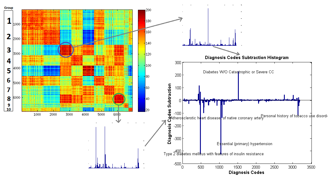
Figure 3: Similarity matrix and diagnosis codes histograms. The matrix represents resemblances of pairwise patients while histograms show quantity of diagnoses. Group 3 and Group 8 look highly overlapping at the diagnosis level (top-left figure), but in fact, their clinical conditions are significantly different when we subtract the two histograms (lower-right figure). (Best viewed in colors).

(a) Tag cloud of diagnosis descriptions.

(b) Age histogram.

Figure 4: Type I diabetes mellitus: Primary diagnoses and age distribution. Two figures confirms the existing knowledge that Type I diabetes mellitus often occurs in the younger population.

(a) Tag cloud of diagnosis descriptions.

(b) Age histogram.

Figure 5: Type II Diabetes mellitus: Primary diagnoses and age distribution. We can see that the age distribution is distinct from the Type I group.

For quantitative evaluation, we calculate the Rand-index [58] to assess the quality of resulting clusters, given that we do not have cluster labels. The Rand-index is the pairwise accuracy between any two patients. To judge whether two patients share the same cluster, we consult the diagnosis code hierarchy of the ICD-10 [33]. We use hierarchical assessment since a diagnosis code may have multiple levels. E11.12, for example, has two levels: E11 and E11.12. The lower level code specifies disease more clearly whilst the higher is more abstract. Therefore we have two ways for pairwise judgement: the Jaccard coefficient (Par. 4.1.2) and code ‘cluster’ which is the grouping of codes that belong to the same disease class, as specified by the latest WHO standard ICD-10. At the lowest level, two patients are considered similar if the two corresponding code sets are sufficiently overlapping, i.e., their Jaccard coefficient is greater than a threshold $\rho_{2}\in(0,1)$. At higher level, on the other hand, we consider two patients to be clinically similar if they share higher level diabetes code of the same code ‘cluster’. For instance, two patients with two codes E11.12 and E11.20 are similar at the level E11, but they are dissimilar at the lower level. Note that this hierarchical division is for evaluation only. We use codes at the lowest level as replicated softmax units in our model (Section 4.1.1).

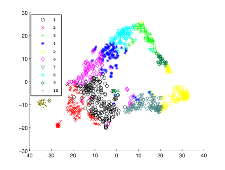
(a)

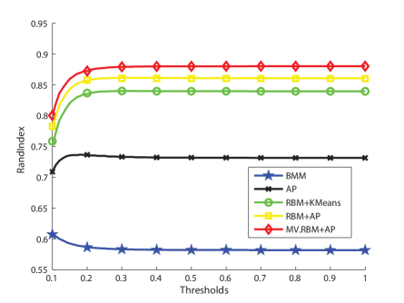
(b)

Figure 6: Visualisation and quantitative assessment of clusters. (a) t-SNE [84] projection on $2,000$ latent profiles. Groups are labelled by the outputs of the AP. (Best viewed in colors). (b) Rand-index curves in patient clustering. AP: affinity propagation, BMM: Bayesian mixture model, RBM: MV.RBM with diagnosis codes only.

Figure 6b reports the Rank-indices with respect to the assessment at the lowest level in the ICD-10 hierarchy for clustering methods with and without MV.RBM pre-processing. At the next ICD-10 level, the MV.RBM/AP achieves a Rand-index of $0.6040$, which is, again, the highest among all methods, e.g., using the RBM/AP yields the score of $0.5870$, and using AP on diagnosis codes yields $0.5529$. This clearly demonstrates that (i) MV.RBM latent profiles would lead to better clustering that those using diagnosis codes directly, and (ii) modelling mixed-types would be better than using just one input type (e.g., the diagnosis codes).

Disease Prediction.

The prediction results are summarised in Figure 7, where the ROC curve of the MV.RBM is compared against that of the baseline using $k$-nearest neighbours ($k$-NN). The $k$-NN approach to disease ranking is as follows: For each patient, a neighbourhood of the $50$ most similar patients is collected based on the Jaccard coefficient over sets of unique diagnoses. The diagnoses are then ranked according to their occurrence frequency within the neighbourhood. As can be seen from the figure, the latent profile approaches outperform the $k$-NN method. The MV.RBM with contextual information such as age, gender and region-of-birth proves to be useful. In particular the the areas under the ROC curve (AUC) of the MV.RBMs are $0.84$ (with contextual information) and $0.82$ (without contextual information). These are clearly better than the score obtained by $k$-NN, which is $0.77$.

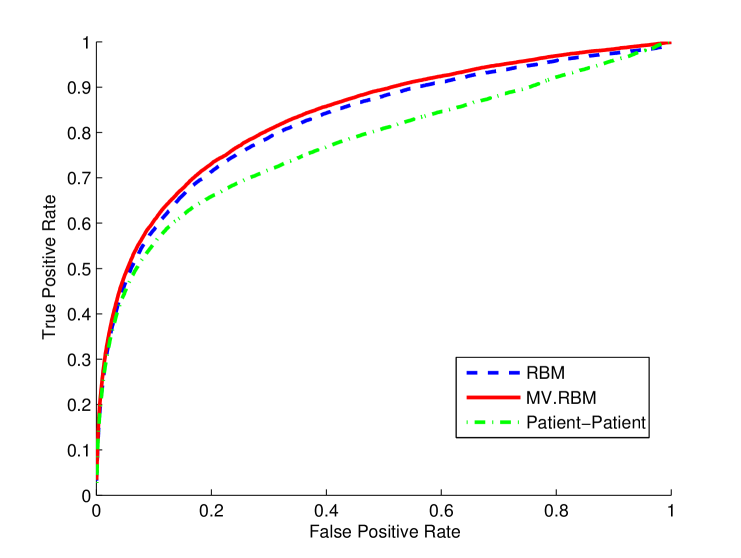
Figure 7: ROC curves in disease prediction. RBM is MV.RBM with diagnosis codes only; Patient-Patient is the $k$-nearest neighbours method. Best viewed in colors.

4.2 Image Retrieval

Images are typically retrieved based on the distance from the query image. Thus the retrieval quality depends critically on how the images are represented and the distance metric operating on the representation space. Standard vector-based representations may involve colour histograms or visual descriptors; and distance metrics can be those working in the vector space. However, they suffer from important drawbacks. First, there are no simple ways to integrate multiple representations (e.g., histograms and bag-of-words) and multiple modalities (e.g., visual words and textual tags). Furthermore, designing a representation separately from distance metric is sup-optimal – it takes time to search for the best distance metric for a given representation. And third, using low-level features may not capture well the high-level semantics of interest, leading to poor retrieval quality if the visual features are similar and the objects are different. For example, it can be easy to confuse between a lion and a wolf if we rely on the textures and colours alone.

In this problem, our solution is to learn both the higher representation and the distance metric specifically for the retrieval task. The higher representation would capture the regularities and factors of variation in the data space from multiple lower feature types and modalities. At the same time, the representation would lead to small distances between conceptually related objects and large distances between those unrelated. To that end, we integrate structured sparsity (Section 3.3) and distance metric learning (Section 3.4) into MV.RBM (Section 3.2). The MV.RBM is a probabilistic architecture capable of integrating several data types into a homogeneous “latent” representation in an unsupervised fashion. Our methods include the introduction of the counting of visual/textual words [60] and the group-wise sparsity [44] into the model. During the training phase, the model learning is regularised in the way that the information theoretic distances on the latent representation between intra-concept images are minimised and those between inter-concept images are maximised. During the testing phase, the learned distance metrics are then used for retrieving similar images.

We demonstrate the effectiveness of the proposed method on the NUS-WIDE data. This data is particularly rich: Each image has multiple visual representations, sometimes social tags, and one or more manually annotated high-level concepts. We run experiments on two subsets. The first is the well-studied $13$ animal subset in which we show that our method is competitive against recent state-of-the-arts. The second subset contains $20,000$ single-concept images. We obtain $79.5\%$ improvement on mean average precision (MAP) over the standard nearest neighbours approach and $45.7\%$ increase on the normalised discounted cumulative gain (NDCG).

Section 4.2.1 presents the Mixed-Variate RBM with group-wise sparsity and metric learning for image retrieval. We show empirical evaluation on the two NUS-WIDE subsets in Section 4.2.2.

4.2.1 Integrated framework

We present our framework of simultaneous learning of sparse data representation and distance metric for image retrieval tasks. The framework has three components: (i) a mixed-variate machine that maps multiple feature types and modalities into a homogeneous higher representation, (ii) a regulariser that promotes structured sparsity on the learned representation, and (iii) an information-theoretic distance operating on the learned representation. To what follows, we involve the structure sparsity in Section 3.3 and metric learning in Section 3.4 to the unsupervised learning parameters of MV.RBM in Section 3.2. Our approach has three goals: Capturing the joint representation of visual and textual features by maximising the data likelihood $\mathcal{L}\left(\boldsymbol{v};\psi\right)=\sum_{\boldsymbol{h}}P\left(\boldsymbol{h},\boldsymbol{v};\psi\right)$, enhancing structural sparsity through minimising $\mathcal{R}\left(\boldsymbol{v}\right)$, and regularising intra-concept and inter-concept distance metrics $\mathcal{D}_{\mathsf{N}\left(f\right)}$ and $\mathcal{D}_{\bar{\mathsf{N}}\left(f\right)}$. The objective function is now the following regularised likelihood

$$\mathcal{L}_{reg}=\sum_{f}\log\mathcal{L}\left(\boldsymbol{v}^{\left(f\right)};\psi\right)-\alpha\mathcal{R}\left(\boldsymbol{v}\right)-\beta\left(\sum_{f}\mathcal{D}_{\mathsf{N}\left(f\right)}-\sum_{f}\mathcal{D}_{\bar{\mathsf{N}}\left(f\right)}\right)$$

where $\alpha\geq 0$ is the regularising constant for sparsity, $\beta\geq 0$ is the coefficient to control the effect of distance metrics. Maximising this regularised likelihood is equivalent to simultaneously maximising the data likelihood $\mathcal{L}\left(\boldsymbol{v};\psi\right)$, minimising the regularisation function $\mathcal{R}\left(\boldsymbol{v}\right)$, minimising the neighbourhood distance $\mathcal{D}_{\mathsf{N}\left(f\right)}$ and maximising the non-neighbourhood distance $\mathcal{D}_{\bar{\mathsf{N}}\left(f\right)}$.

In Section 3, the derivatives of regularised likelihood with respect to parameters are all specified. Consequently, we perform stochastic gradient ascent to update parameters as follows

$$\psi\leftarrow\psi+\lambda\left(\frac{\partial}{\partial\psi}\mathcal{L}_{reg}\right)$$

for some learning rate $\lambda>0$.

4.2.2 Empirical evaluations

In this task, we quantitatively evaluate our method on two real datasets. Both datasets are subsets selected from the NUS-WIDE dataset [10], which was collected from Flickr. The NUS-WIDE dataset includes $269,648$ images which are associated with $5,018$ unique tags. There are $81$ concepts in total. For each image, six types of low-level features [10] are extracted, including $64$-D color histogram in LAB color space, $144$-D color correlogram in HSV color space, $73$-D edge direction histogram, $128$-D wavelet texture, $225$-D block-wise LAB-based color moments extracted over $5\times 5$ fixed grid partitions and $500$-D bag-of-word (BOW) based on SIFT descriptions.

For training our model, mapping parameters $\boldsymbol{W}$ are randomly initialised from small normally distributed numbers, i.e. Gaussian $\mathcal{N}\left(0;0.01\right)$, and biases $\left(\boldsymbol{a},\boldsymbol{b}\right)$ are set to zeros. To enhance the speed of training, we divide training images into small “mini-batches” of $B=100$ images. Hidden and visible learning rates are fixed to $0.02$ and $0.3$, respectively. Parameters are updated after every mini-batch and the learning finishes after $100$ scans through the whole data. Once parameters have been learned, images are projected onto the latent space using Eq. (4). We set the number of hidden groups $M$ to the expected number of groups (e.g., concepts), and the number of hidden units $K$ is multiple of $M$. The retrieved images are ranked based on the negative KL-div on these latent representations. We repeat $10$ times and report the mean and standard deviation of the performance measures.

Retrieving Animals.

The first subset is the NUS-WIDE animal dataset which contains $3,411$ images of $13$ animals - squirrel, cow, cat, zebra, tiger, lion, elephant, whale, rabbit, snake, antler, wolf and hawk. Figure 8 shows example images of each category. Out of $3,411$ images, $2,054$ images are used for training and the remaining for testing. In the testing phase, each test image is used to query images in training set to receive a list of images ranked basing on similarities. These settings are identical to those used in previous work [25, 26, 9]. For our methods, the similarity measure is negative symmetric Kullback-Leibler divergence (KL-div) learned from data (Section 4.2.1). The retrieval performance is evaluated using Mean Average Precision (MAP) over all received images in training set. Two images are considered similar if they depict the same type of animal.

squirrel	cow	cat	tiger	whale	rabbit	snake
zebra	lion	elephant		antler	wolf	hawk

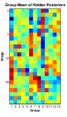
Figure 8: Example images of each species in NUS-WIDE animal dataset. The last column shows the group mean of hidden posteriors by colours, one line per image. The red cells illustrate higher values whilst the blue denote the lower. It is clear that 4 groups of 6 consecutive images form 4 strips in different groups (9,6,1,8).

In this experiment, we concatenate first five histogram features of each animal image into a long vector and ignore BOW features to fairly compare with recent work. Thus we treat elements of the vector as Gaussian units and normalise them across all training images to obtain zeros mean and unit standard variance. Note that the MV.RBM here reduces to the plain RBM with single Gaussian type.

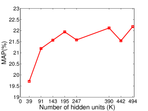
(a)

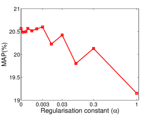
(b)

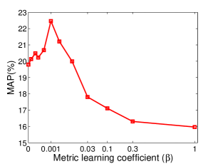
(c)

Figure 9: The MAP performance (%) as functions of the hyper-parameters: (Left) The number of hidden units $K$ (with $\alpha=0.003$ and $\beta=0.001$); (Middle) The regularisation constant $\alpha$ (with $K=195$); (Right) The metric learning coefficient $\beta$ (with $K=195$ and $\alpha=0.003$).

To find the best setting of the hyper-parameters $\alpha,\beta$ and $K$, we perform initial experiments with varying values. Figure 9 reports the MAP performance (%) with respect to these values. Here $\alpha=0$ means no sparsity constraint and $\beta=0$ means no metric learning. As can be seen from the left figure, the performance stops increasing after some certain hidden size. Adding certain amount of sparsity control slightly improves the result (see the middle figure). A much stronger effect is due to metric learning, as shown in the right figure. From these observations, we choose $K=195$ (15 units per group), $\alpha=0.003$ and $\beta=0.001$.

		$k$-NN
lion	wolf	lion	wolf	lion
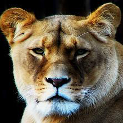
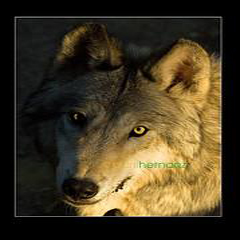
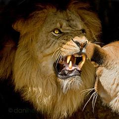
RBM
lion	wolf	lion	lion	wolf
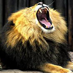
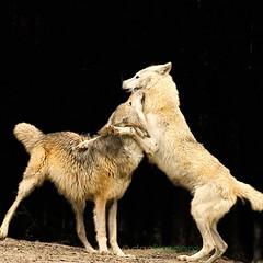
RBM+SG
lion	lion	wolf	lion	lion
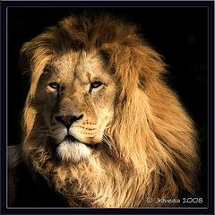
RBM+SG+ML
lion	lion	lion	lion	lion

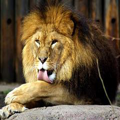
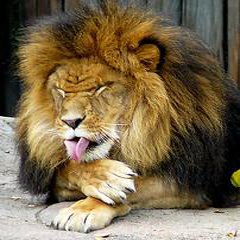
Figure 10: Retrieved images for query image of a lion in testing set. $k$-NN: $k$-nearest neighbours, RBM+SG+ML: RBM with sparse group, metric learning. First column is the queried images. Blue titles are right retrieval whilst the red are wrong. Four retrieved images are sorted in descent order of similarities from left to right.

Figure 10 shows how structured sparsity and metric learning contributes to the higher retrieval quality. The naive nearest neighbour on concatenated normalised features would confuse a wolf with the query of lion, possibly due to the similar colour profiles. The standard RBM admits the same error suggesting that learning just regularities is not enough. Adding structured sparsity (RBM+SG) corrects one error and using learned metric (RBM+SG+ML) would correct all the errors.

Table 1: Image retrieval results to compare with recent state-of-the-art multiview learning and hierarchical modelling techniques on NUS-WIDE animal dataset. RBM+SG+ML is RBM with latent sparse groups and metric learning.

Method	MAP
DWH [9]	0.153
TWH [9]	0.158
MMH [9]	0.163
NHFA-GGM (approx.) [25]	0.179±0.013
Proposed NHFA-GGM [26]	0.195±0.013
RBM	0.199±0.001
RBM+SG	0.206±0.002
RBM+SG+ML	0.252±0.002

Finally, Table 1 presents the MAP results of our methods (RBM, RBM with sparse group (SG) and with metric learning (ML)) in comparison with recent work [9, 25, 26] on the NUS-WIDE animal dataset. It is clear that RBM and RBM with SG are competitive against all previous methods; and RBM integrated with SG and ML significantly outperforms state-of-the-art approaches.

Retrieving Individual Concepts.

In the second experiment, we aim to demonstrate the capability of our method to handle heterogeneous types of features and larger data. We randomly pick 10,000 images for training and 10,000 for testing. Each image in this subset has exactly one concept and altogether, they cover the entire 81 concepts of the NUS-WIDE dataset. Six visual features (1 bag-of-word and 5 histogram-like) and associated social tags, limited to 1,000, of each image are taken. The MV.RBM encodes 5 histogram features as Gaussian, social tags as binary and BOW as Poisson units. We further transform counts into $log$ space using $\left[log\left(1+\textnormal{count}\right)\right]$.

Besides MAP score, we also compute the Normalized Discounted Cumulative Gain (NDCG) [34] for evaluation. Here we only use the top 100 similar images for calculating MAP and top 10 images for computing NDCG. We create 2 baselines and 4 versions of our approach to show the improvement of the MV.RBM when adding sparse groups and metric learning (MV.RBM+SG+ML). The first baseline is to employ $k$-NN method on concatenated feature vectors. First features are normalised to zeros mean and unit vector over images to eliminate the differences in dimensionality and scale. The second baseline is fusion of multiple plain RBMs, each of which is type specific, i.e., BOW as Poisson, visual histograms as Gaussian and textual tags as binary. For each type of RBM, visible input data is mapped into binary latent representation. Then these latent representations are concatenated into a single latent representation.

The first version (RBM+SG) is the second baseline with group-wise sparsity (Section 3.3). The second version (MV.RBM) jointly models all 7 types of features. The third version (MV.RBM+SG) is MV.RBM with $81$ sparse groups (Section 3.3). And finally, the proposed solution (MV.RBM+SG+ML) integrates both the sparsity and the metric learning into the MV.RBM.

Table 2: Comparison of image retrieval results with 4 baselines on NUS-WIDE single label subset. (model)+SG+ML means (model) is integrated with sparse groups and metric learning. MAP@100 is evaluated at top 100 similar images. N@10 = NDCG estimated at top 10 results. ($\uparrow$%) denotes improved percentage.

Method	MAP@100 ($\uparrow$%)	N@10 ($\uparrow$%)
$k$NN	0.283	0.466
RBM	0.381±0.001(+34.6)	0.565±0.001(+21.2)
RBM+SG	0.402±0.035(+42.1)	0.584±0.001(+25.3)
MV.RBM	0.455±0.002 (+60.8)	0.631±0.002 (+35.4)
MV.RBM+SG	0.483±0.002 (+70.7)	0.668±0.002 (+43.4)
MV.RBM+SG+ML	0.508±0.002(+79.5)	0.679±0.001(+45.7)

Different from the first experiment, we query within testing set for each testing image. Table 2 reports the retrieval results of all RBM models. Again, it demonstrates that (i) representation learning, especially when it comes to fusing multiple feature types and modalities, is highly important in image retrieval, (ii) adding structured sparsity can improve the performance, and (iii) distance metric, when jointly learned with representation, has significant effect on the retrieval quality. In particular, the improvement over the $k$-NN when using the proposed method is significant: MAP score increases by $79.5\%$ and NDCG score by $45.7\%$.

5 Discussion and Future Works

5.1 Drawbacks and Future Plans

Referring back to previous sections, our principal direction concentrates on learning a better representation which critically influences the performance of machine learning methods. However, we have explored “shallow” architectures (e.g., generative and discriminative models with only one hidden layer, Support Vector Machines) which are too simple to model mixed data. Such shallow architectures are unable to capture several complex types of multisource data [3]. Thus constructing a deep architecture has been obtaining a lot of attention. One of the typical examples is multilayer neural networks. Unfortunately, they requires a huge amount of labelled data and often are trapped at poor local optima.

Hinton et al. [28] propose a deep generative model known as Deep Belief Network (DBN). They also contribute an unsupervised learning algorithm which helps train DBN quickly. Later, the generalised model of RBM called Deep Boltzmann Machine (DBM) is introduced as a deep architecture. Since then, they have opened the door to a novel research direction called “deep learning”. Applications of deep learning then vary in speech recognition [48], object recognition [29, 11, 37] and statistical machine translation [64]. In such fields, deep learning models often achieve state-of-the-art results or potential outcomes comparable to the supremacy rivals. Additionally, Deep Auto-Encoder is introduced to enhance the data representations by fine-tuning in unsupervised fashion. Recently, deep learning has also been applied to multimodal learning using DBN [51] and DBM [71].

Interestingly, RBM-based models can easily be stacked to form a deep architecture such as Deep Belief Network (DBN). It also has been proved that building a deeper model by stacking more hidden layers increases the log probabilities of the data [28]. Besides, the key feature of this deep architecture is greedy layer-wise training that can be repeated several times to learn a deep hierarchical model. After initialising weights for all layers by using multiple RBMs, all parameters of this hierarchical model are fine-tuned by back-propagation similar to neural networks. The advantages of unsupervised pretraining with respect to deep architectures are empirically proved in [19]. In addition, our proposed models basing on RBM and MV.RBM demonstrate their capabilities in latent patient profile modelling in medical data analysis and representation learning for image retrieval according to Sec. 4. Thanks to promising perspective, we have grasped motivations and preliminary guarantees of success to extend our proposed models to deep versions.

Another research direction is to explore temporal information in mixed data such as sequential frames in video, serial signals in audio and disease escalation of patients over time. In this field, the mixed-variate property can be integrated into existing models including conditional RBM and temporal RBM [75].

5.2 Future Objectives

Our proposed models still focus on learning representation in latent space for mixed data. The aims are now furthered to learn hierarchical latent representations for mixed data and integrate temporal information into deep architecture. The detailed objectives are to:

• Improve deep architectures to tackle multitype and multimodal data. The deep here are built for classification, regression and encoding, decoding purposes;

• Integrate structured sparsity and distance metric learning into deep architectures as well as investigate how many levels and which levels should be enhanced by structured sparsity and distance metric; and

• Upgrade conditional and temporal RBMs to mixed-variate versions and build deep architectures basing on these mixed-variate models.

5.3 Significance and benefits

The significance of our further research can be recognised in two fields: machine learning and life supports. In machine learning, our main contributions are: (i) Implementing versatile RBM-based machineries to handle mixed data; (ii) Novel extension and application of a powerful data mining tool, Mixed-Variate RBM, to deep architectures and (iii) Constructing robust hierarchical latent representations with sparsity structures and distance metric learning. In life supports, the significance of our work lies in: (i) Building a robust framework that is able to support healthcare centres and clinicians delivering outcomes that can integrate with their operations to enhance clinical efficiencies. Using such systems, the management and supervision on diabetes patients in particular as well as other kinds of diseases patients in general would have the potential to improve; (ii) Providing a powerful representation learning machinery for real applications including face recognition, object classification and image retrieval.

5.4 Methodology

In order to achieve the objectives outlined in Sec. 5.2, we are planning to implement the following methods:

• Mixed-variate deep architecture. In this architecture, the lowest layer employs a Mixed-Variate RBM (see Sec. 3.2) to model mixed-data with binary units in hidden layer. Next, standard binary RBMs are stacked to build higher layers. The lowest layer and higher layers form a block which can be pretrained layer-by-layer to find good regions in parameter space [29]. After pretraining stage, there are two approaches for the late training phase depending on the purpose the model serves. For classification and regression problems, we add another layer on the recent highest layer of the deep model. The additional layer contains the output units such as softmax, logistic units for classification and real units for regression. For data reconstruction, the recent deep model is unrolled in order to create an autoencoder. This autoencoder is in palindromic form with the last layer representing the data. Finally, following this late training phase, we fine-tune the last model using backpropagation, minimising error objective function or maximising log-likelihood function, to figure out optimal set of parameters [29]. Note that, we must resort to specific objective function for each type of output units such as Poisson log-likelihood function for count data, cross-entropy error for binary value and Gaussian log-likelihood function, the same as mean square error, for real one.

• Deep learning with structured sparsity and distance metric. Hierarchical representations can be learned by deep architectures. These representations are retrieved using the output of units at level-based layer. Machine learning methods then can be applied to the representation at the last layer. Obviously, the better the last representation is, the more superior results we can obtain. According to Sec. 4.2.1, we have successfully integrated structured sparsity and distance metric learning into the latent representation of MV.RBM. The sparsity and distance metric are enhanced during the training phase. Similarly, we can deploy this way to the pretraining and fine-tuning stages of deep architectures. However, we need to investigate which layers we should integrate these things into because the integration can be applied to either any single layer or their combinations.

• Mixed-variate conditional and temporal RBMs. The standard RBM-based frameworks only model static frames of data. They have not taken temporal information into account. Considering temporal as well as time series factor, the data should be sorted by time order. The data, then, is splited into timing windows (time slices). We are now able to model temporal dependencies by treating previous time slices as additional visible variables. A model called Temporal RBM (TRBM) is proposed in order to add directed connections from the past configurations of visible and hidden units [72]. There are three kinds of connections in full TRBM: connections among the hidden variables, connections among the visible variables and connections among the visible and hidden variables. Full TRBM can even have the fourth kind of connections from the past hidden configurations to the current visible units. In fact, the model is already powerful enough without the fourth connections. To simplify the full TBRM, Taylor et al. [74] ignore previous hidden configurations and connections among hidden units. They only add two types of directed connections: autoregressive connections from the last $N$ states of visible units to the current visible states, and connections from the last $M$ states of visible units to the current hidden states. These connections transform RBM into Conditional RBM (CRBM). Because all states of visible units in CRBM and TRBM act as visible ones in the standard RBM, we can use each state of visible units to model mixed data like the way MV.RBM has performed. Once CRBM and TRBM successfully model mixed data, multiple layers of them can be stacked to build deep architectures.

6 Conclusion

To summarise, we have provided an overview of mixed data analysis in statistics and machine learning. We have reviewed related literatures on three main approaches: applying techniques on original features; non-probabilistically transforming data to higher-level representations and modelling mixed data using latent variable frameworks. Our main approaches are to utilise Restricted Boltzmann Machine (RBM) and its variants, bipartite undirected graphical models with visible layer observing the data and hidden layer representing the latent representation. We have introduced firstly, our extensions of parameter sharing and balancing and secondly, integrated structured sparsity and distance metric learning into RBM and Mixed-Variate RBM (MV.RBM). We then applied our proposed models in various applications including latent patient profile modelling in medical data analysis and representation learning for image retrieval. The experimental results demonstrated the models performed better than baseline methods in medical data and outperformed state-of-the-art rivals in image dataset. In future works, we aim to learn hierarchical latent representations for mixed data and integrate temporal information into deep architecture. The significance of our further research would be recognised in two fields: machine learning and life supports.

References

- [1] David H Ackley, Geoffrey E Hinton, and Terrence J Sejnowski. A learning algorithm for boltzmann machines. Cognitive science, 9(1):147–169, 1985.
- [2] Stéphane Ayache, Georges Quénot, and Jérôme Gensel. Classifier fusion for SVM-based multimedia semantic indexing. In Advances in Information Retrieval, pages 494–504. Springer, 2007.
- [3] Yoshua Bengio. Learning deep architectures for AI. Foundations and Trends in Machine Learning, 2(1):1–127, 2009. Also published as a book. Now Publishers, 2009.
- [4] David M Blei, Andrew Y Ng, and Michael I Jordan. Latent dirichlet allocation. the Journal of machine Learning research, 3:993–1022, 2003.
- [5] Thomas Bodenheimer, Ellen Chen, and Heather D Bennett. Confronting the growing burden of chronic disease: can the us health care workforce do the job? Health Affairs, 28(1):64–74, 2009.
- [6] Bernhard E Boser, Isabelle M Guyon, and Vladimir N Vapnik. A training algorithm for optimal margin classifiers. In Proc. of the fifth annual workshop on Computational learning theory, pages 144–152. ACM, 1992.
- [7] P. J. Catalano. Bivariate modelling of clustered continuous and ordered categorical outcomes. Statistics in medicine, 16(8):883–900, 1997.
- [8] Chih-Chung Chang and Chih-Jen Lin. A Practical Guide to Support Vector Classification. ACM Trans. Intell. Syst. Technol., 2(3):27:1–27:27, May 2011.
- [9] N. Chen, J. Zhu, and E.P. Xing. Predictive subspace learning for multi-view data: a large margin approach. Advances in Neural Information Processing Systems, 24, 2010.
- [10] Tat-Seng Chua, Jinhui Tang, Richang Hong, Haojie Li, Zhiping Luo, and Yan-Tao Zheng. Nus-wide: A real-world web image database from national university of singapore. In Proc. of ACM Conf. on Image and Video Retrieval (CIVR’09), Santorini, Greece, July 8-10 2009.
- [11] Dan Ciresan, Ueli Meier, and Jürgen Schmidhuber. Multi-column deep neural networks for image classification. In Proc. of Computer Vision and Pattern Recognition (CVPR), pages 3642–3649. IEEE, 2012.
- [12] Corinna Cortes and Vladimir Vapnik. Support-vector networks. Machine learning, 20(3):273–297, 1995.
- [13] John N Darroch, Steffen L Lauritzen, and TP Speed. Markov fields and log-linear interaction models for contingency tables. The Annals of Statistics, pages 522–539, 1980.
- [14] A. R. de Leon and B. Wu. Copula-based regression models for a bivariate mixed discrete and continuous outcome. Statistics in Medicine, 30(2):175–185, 2011.
- [15] Scott Deerwester, Susan T. Dumais, George W Furnas, Thomas K Landauer, and Richard Harshman. Indexing by latent semantic analysis. Journal of the American society for information science, 41(6):391–407, 1990.
- [16] David B. Dunson. Bayesian latent variable models for clustered mixed outcomes. Journal of the Royal Statistical Society. Series B (Statistical Methodology), 62(2):pp. 355–366, 2000.
- [17] David B Dunson. Dynamic latent trait models for multidimensional longitudinal data. Journal of the American Statistical Association, 98(463):555–563, 2003.
- [18] D.B. Dunson and A.H. Herring. Bayesian latent variable models for mixed discrete outcomes. Biostatistics, 6(1):11, 2005.
- [19] Dumitru Erhan, Yoshua Bengio, Aaron Courville, Pierre-Antoine Manzagol, Pascal Vincent, and Samy Bengio. Why does unsupervised pre-training help deep learning? J. Mach. Learn. Res., 11:625–660, March 2010.
- [20] Ronald A Fisher. The use of multiple measurements in taxonomic problems. Annals of eugenics, 7(2):179–188, 1936.
- [21] Yoav Freund and David Haussler. Unsupervised learning of distributions on binary vectors using two layer networks. Technical report, Santa Cruz, CA, USA, 1994.
- [22] Brendan J. Frey and Delbert Dueck. Clustering by passing messages between data points. Science, 315:972–976, 2007.
- [23] P.V. Gehler, A.D. Holub, and M. Welling. The rate adapting poisson model for information retrieval and object recognition. In Proceedings of the 23rd international conference on Machine learning, pages 337–344. ACM, 2006.
- [24] Jacob Goldberger, Sam Roweis, Geoff Hinton, and Ruslan Salakhutdinov. Neighbourhood components analysis. In Advances in Neural Information Processing Systems 17, pages 513–520. MIT Press, 2004.
- [25] S. Gupta, D. Phung, B. Adams, and S. Venkatesh. A bayesian framework for learning shared and individual subspaces from multiple data sources. Advances in Knowledge Discovery and Data Mining, pages 136–147, 2011.
- [26] S.K. Gupta, D. Phung, and S. Venkatesh. A slice sampler for restricted hierarchical beta process with applications to shared subspace learning. In Uncertainty in Artificial Intelligence, pages 316–325. AUAI Press Corvallis, Oregon, 2012.
- [27] T. Hertz, A. Bar-Hillel, and D. Weinshall. Learning distance functions for image retrieval. In Computer Vision and Pattern Recognition, 2004. CVPR 2004. Proceedings of the 2004 IEEE Computer Society Conference on, volume 2, pages II–570 – II–577 Vol.2, june-2 july 2004.
- [28] G.E. Hinton, S. Osindero, and Y.W. Teh. A fast learning algorithm for deep belief nets. Neural computation, 18(7):1527–1554, 2006.
- [29] Geoffrey Hinton and Ruslan Salakhutdinov. Reducing the dimensionality of data with neural networks. Science, 313(5786):504 – 507, 2006.
- [30] Geoffrey E. Hinton. Training products of experts by minimizing contrastive divergence. Neural Computation, 14(8):1771–1800, 2002.
- [31] Thomas Hofmann. Probabilistic latent semantic analysis. In Proceedings of the Fifteenth conference on Uncertainty in artificial intelligence, pages 289–296. Morgan Kaufmann Publishers Inc., 1999.
- [32] John J Hopfield. Neural networks and physical systems with emergent collective computational abilities. Proceedings of the national academy of sciences, 79(8):2554–2558, 1982.
- [33] World Health Organization: ICD-10th, 2010. accessed September 2012.
- [34] Kalervo Järvelin and Jaana Kekäläinen. Cumulated gain-based evaluation of ir techniques. ACM Trans. Inf. Syst., 20(4):422–446, October 2002.
- [35] Andrew E. Johnson and Martial Hebert. Using spin images for efficient object recognition in cluttered 3d scenes. Pattern Analysis and Machine Intelligence, IEEE Transactions on, 21(5):433–449, 1999.
- [36] Ian T Jolliffe. Principal component analysis, volume 487. Springer-Verlag New York, 1986.
- [37] Alex Krizhevsky, Ilya Sutskever, and Geoff Hinton. Imagenet classification with deep convolutional neural networks. In Advances in Neural Information Processing Systems 25, pages 1106–1114, 2012.
- [38] Steffen L Lauritzen. Graphical models, volume 17. Oxford University Press, 1996.
- [39] Nicolas Le Roux, Nicolas Heess, Jamie Shotton, and John Winn. Learning a generative model of images by factoring appearance and shape. Neural Computation, 23(3):593–650, 2011.
- [40] Yann LeCun, Léon Bottou, Yoshua Bengio, and Patrick Haffner. Gradient-based learning applied to document recognition. Proceedings of the IEEE, 86(11):2278–2324, 1998.
- [41] Yann LeCun, Sumit Chopra, Raia Hadsell, Marc’Aurelio Ranzato, and Fu-Jie Huang. A tutorial on energy-based learning. In G. Bakir, T. Hofman, B. Schölkopf, A. Smola, and B. Taskar, editors, Predicting Structured Data. MIT Press, 2006.
- [42] Daniel D Lee and H Sebastian Seung. Learning the parts of objects by non-negative matrix factorization. Nature, 401(6755):788–791, 1999.
- [43] H. Lee, C. Ekanadham, and A. Ng. Sparse deep belief net model for visual area v2. Advances in neural information processing systems, 20:873–880, 2008.
- [44] Heng Luo, Ruimin Shen, Changyong Niu, and Carsten Ullrich. Sparse group restricted boltzmann machines. In Twenty-Fifth AAAI Conference on Artificial Intelligence, 2011.
- [45] C. McCulloch. Joint modelling of mixed outcome types using latent variables. Statistical Methods in Medical Research, 17(1):53, 2008.
- [46] A-R Mohamed and Geoffrey Hinton. Phone recognition using restricted boltzmann machines. In Acoustics Speech and Signal Processing (ICASSP), 2010 IEEE International Conference on, pages 4354–4357. IEEE, 2010.
- [47] Abdel-rahman Mohamed, George Dahl, and Geoffrey Hinton. Deep belief networks for phone recognition. In NIPS Workshop on Deep Learning for Speech Recognition and Related Applications, 2009.
- [48] Abdel-rahman Mohamed, George E Dahl, and Geoffrey Hinton. Acoustic modeling using deep belief networks. IEEE Transactions on Audio, Speech, and Language Processing, 20(1):14–22, 2012.
- [49] Jared S Murray, David B Dunson, Lawrence Carin, and Joseph E Lucas. Bayesian gaussian copula factor models for mixed data. Journal of the American Statistical Association, (just-accepted), 2013.
- [50] V. Nair and G.E. Hinton. Rectified linear units improve restricted boltzmann machines. In Proc. 27th International Conference on Machine Learning, pages 807–814. Omnipress Madison, WI, 2010.
- [51] J. Ngiam, A. Khosla, M. Kim, J. Nam, H. Lee, and A. Y. Ng. Multimodal deep learning. In ICML, 2011.
- [52] Tu Dinh Nguyen, Truyen Tran, Dinh Phung, and Svetha Venkatesh. Latent patient profile modelling and applications with mixed-variate restricted boltzmann machine. In Jian Pei, VincentS. Tseng, Longbing Cao, Hiroshi Motoda, and Guandong Xu, editors, Proceedings of the 17th Pacific-Asia Conference on Knowledge Discovery and Data Mining (PAKDD), volume 7818 of Lecture Notes in Computer Science, pages 123–135, Gold Coast, Australia, 2013. Springer-Verlag Berlin Heidelberg.
- [53] Tu Dinh Nguyen, Truyen Tran, Dinh Phung, and Svetha Venkatesh. Learning sparse latent representation and distance metric for image retrieval. In Proceedings of IEEE International Conference on Multimedia and Expo (ICME), pages 1–6, San Jose, California, USA, 2013.
- [54] Bruno A Olshausen et al. Emergence of simple-cell receptive field properties by learning a sparse code for natural images. Nature, 381(6583):607–609, 1996.
- [55] Bruno A Olshausen, David J Field, et al. Sparse coding with an overcomplete basis set: A strategy employed by vi? Vision research, 37(23):3311–3326, 1997.
- [56] World Health Organization. Diabetes (2012), 2012. accessed September 2012.
- [57] J. Paisley and L. Carin. Nonparametric factor analysis with beta process priors. In Proceedings of the 26th Annual International Conference on Machine Learning, pages 777–784. ACM, 2009.
- [58] W.M. Rand. Objective criteria for the evaluation of clustering methods. Journal of the American Statistical Association, pages 846–850, 1971.
- [59] Marc Aurelio Ranzato and Geoffrey E Hinton. Modeling pixel means and covariances using factorized third-order boltzmann machines. In Computer Vision and Pattern Recognition (CVPR), 2010 IEEE Conference on, pages 2551–2558. IEEE, 2010.
- [60] R. Salakhutdinov and G. Hinton. Semantic hashing. In SIGIR Workshop on Information Retrieval and Applications of Graphical Models, volume 500. ACM Special Interest Group on Information Retrieva, 2007.
- [61] R. Salakhutdinov and GE Hinton. Replicated softmax: an undirected topic model. Advances in Neural Information Processing Systems, 22:1607–1614, 2009.
- [62] R. Salakhutdinov, A. Mnih, and G. Hinton. Restricted boltzmann machines for collaborative filtering. In Proceedings of the 24th international conference on Machine learning, pages 791–798. ACM, 2007.
- [63] Mary Dupuis Sammel, Louise M. Ryan, and Julie M. Legler. Latent variable models for mixed discrete and continuous outcomes. Journal of the Royal Statistical Society. Series B (Methodological), 59(3):pp. 667–678, 1997.
- [64] Holger Schwenk, Anthony Rousseau, and Mohammed Attik. Large, pruned or continuous space language models on a gpu for statistical machine translation. In Proc. of the NAACL-HLT 2012 Workshop, pages 11–19. Association for Computational Linguistics, 2012.
- [65] John Shawe-Taylor and Nello Cristianini. Kernel methods for pattern analysis. Cambridge university press, 2004.
- [66] J-Q Shi and S-Y Lee. Latent variable models with mixed continuous and polytomous data. Journal of the Royal Statistical Society: Series B (Statistical Methodology), 62(1):77–87, 2000.
- [67] P. Smolensky. Parallel distributed processing: explorations in the microstructure of cognition, vol. 1. chapter Information processing in dynamical systems: foundations of harmony theory, pages 194–281. MIT Press, Cambridge, MA, USA, 1986.
- [68] C Snoek, Kvd Sande, de O Rooij, B Huurnink, J Uijlings, van M Liempt, M Bugalhoy, I Trancosoy, F Yan, M Tahir, et al. The mediamill trecvid 2009 semantic video search engine. In TRECVID workshop, 2009.
- [69] Cees GM Snoek, Marcel Worring, and Arnold WM Smeulders. Early versus late fusion in semantic video analysis. In Proc. of the 13th annual ACM international Conference on Multimedia (ACMMM), pages 399–402. ACM, 2005.
- [70] Peter X-K Song, Mingyao Li, and Ying Yuan. Joint regression analysis of correlated data using gaussian copulas. Biometrics, 65(1):60–68, 2009.
- [71] Nitish Srivastava and Ruslan Salakhutdinov. Multimodal learning with deep boltzmann machines. In Advances in Neural Information Processing Systems 25, pages 2231–2239, 2012.
- [72] I. Sutskever and G.E. Hinton. Learning multilevel distributed representations for high-dimensional sequences. Proceeding of the Eleventh International Conference on Artificial Intelligence and Statistics, pages 544–551, 2007.
- [73] Dacheng Tao, Xiaoou Tang, Xuelong Li, and Yong Rui. Direct kernel biased discriminant analysis: a new content-based image retrieval relevance feedback algorithm. IEEE Transactions on Multimedia, 8(4):716 –727, Aug 2006.
- [74] Graham W. Taylor, Geoffrey E. Hinton, and Sam Roweis. Modeling human motion using binary latent variables. In Advances in Neural Information Processing Systems, page 2007. MIT Press, 2006.
- [75] Graham W. Taylor, Geoffrey E. Hinton, and Sam T. Roweis. Two distributed-state models for generating high-dimensional time series. J. Mach. Learn. Res., 12:1025–1068, July 2011.
- [76] Yee Whye Teh and Geoffrey E Hinton. Rate-coded restricted boltzmann machines for face recognition. Advances in neural information processing systems, pages 908–914, 2001.
- [77] T. Tieleman. Training restricted boltzmann machines using approximations to the likelihood gradient. In Proceedings of the 25th international conference on Machine learning, pages 1064–1071. ACM New York, NY, USA, 2008.
- [78] Michael E Tipping and Christopher M Bishop. Probabilistic principal component analysis. Journal of the Royal Statistical Society: Series B (Statistical Methodology), 61(3):611–622, 1999.
- [79] Kari Torkkola. Linear discriminant analysis in document classification. In IEEE ICDM Workshop on Text Mining, pages 800–806. Citeseer, 2001.
- [80] T. Tran, D.Q Phung, and S. Venkatesh. Learning boltzmann distance metric for face recognition. In Proc. of IEEE International Conference on Multimedia & Expo, Melbourne, Australia, July 2012.
- [81] Truyen Tran, Dinh Phung, and Svetha Venkatesh. Embedded restricted boltzmann machines for fusion of mixed data. In Proc. of IEEE Int. Conf. on Fusion, Singapore, July 2012.
- [82] Truyen Tran, Dinh Q. Phung, and Svetha Venkatesh. Mixed-variate restricted boltzmann machines. Journal of Machine Learning Research - Proceedings Track, 20:213–229, 2011.
- [83] T. Truyen, D. Phung, and S. Venkatesh. Cumulative restricted Boltzmann machines for ordinal matrix data analysis. In Proceedings of Asian Conference on Machine Learning (ACML), Singapore, November 2012.
- [84] L. van der Maaten and G. Hinton. Visualizing data using t-sne. Journal of Machine Learning Research, 9(Nov):2579–2605, 2008.
- [85] Kilian Q. Weinberger, John Blitzer, and Lawrence K. Saul. Distance metric learning for large margin nearest neighbor classification. In In NIPS. MIT Press, 2006.
- [86] M. Welling, M. Rosen-Zvi, and G. Hinton. Exponential family harmoniums with an application to information retrieval. Advances in neural information processing systems, 17:1481–1488, 2005.
- [87] Eric P. Xing, Rong Yan, and Alexander G. Hauptmann. Mining associated text and images with dual-wing harmoniums. In In Proceedings of the 21st Conference on Uncertainty in Artificial Intelligence. AUAI press, 2005.
- [88] Li-Qun Xu and Yongmin Li. Video classification using spatial-temporal features and pca. In Multimedia and Expo, 2003. ICME’03. Proceedings. 2003 International Conference on, volume 3, pages III–485. IEEE, 2003.
- [89] J. Yu, J. Amores, N. Sebe, and Q. Tian. A new study on distance metrics as similarity measurement. In Multimedia and Expo, 2006 IEEE International Conference on, pages 533 –536, july 2006.
- [90] Wenyi Zhao, Arvindh Krishnaswamy, Rama Chellappa, Daniel L Swets, and John Weng. Discriminant analysis of principal components for face recognition. In Face Recognition, pages 73–85. Springer, 1998.