Future Word Contexts in Neural Network Language Models

Abstract

Recently, bidirectional recurrent network language models (bi-RNNLMs) have been shown to outperform standard, unidirectional, recurrent neural network language models (uni-RNNLMs) on a range of speech recognition tasks. This indicates that future word context information beyond the word history can be useful. However, bi-RNNLMs pose a number of challenges as they make use of the complete previous and future word context information. This impacts both training efficiency and their use within a lattice rescoring framework. In this paper these issues are addressed by proposing a novel neural network structure, succeeding word RNNLMs (su-RNNLMs). Instead of using a recurrent unit to capture the complete future word contexts, a feedforward unit is used to model a finite number of succeeding, future, words. This model can be trained much more efficiently than bi-RNNLMs and can also be used for lattice rescoring. Experimental results on a meeting transcription task (AMI) show the proposed model consistently outperformed uni-RNNLMs and yield only a slight degradation compared to bi-RNNLMs in N-best rescoring. Additionally, performance improvements can be obtained using lattice rescoring and subsequent confusion network decoding.

Index Terms—  Bidirectional recurrent neural network, language model, succeeding words, speech recognition

1 Introduction

Language models (LMs) are crucial components in many applications, such as speech recognition and machine translation. The aim of language models is to compute the probability of any given sentence $\mathcal{W}=(w_{1},w_{2},...,w_{L})$, which can be calculated as

$$P(\mathcal{W})=P(w_{1},w_{2},...,w_{L})=\prod_{t=1}^{L}P(w_{t}|w_{1}^{t-1})$$ (1)

The task of LMs is to calculate the probability of word $w_{t}$ given its previous history $w_{1}^{t-1}=w_{1},w_{2},...,w_{t-1}$. $n$-gram LMs [1] and neural network based language mdoels (NNLMs) [2, 3] are two widely used language models. In $n$-gram LMs, the most recent $n-1$ words are used as an approximation of the complete history, thus

$$P(w_{t}|w_{1}^{t-1})\approx P(w_{t}|w_{t-n+1}^{t-1})$$ (2)

This $n$-gram assumption can also be used to construct a $n$-gram feedforward NNLMs [2]. In contrast, recurrent neural network LMs (RNNLMs) model the complete history via a recurrent connection.

Most of previous work on language models has focused on utilising history information, the future word context information has not been extensively investigated. There have been several attempts to incorporate future context information into recurrent neural network language models. Individual forward and backward RNNLMs can be built, and these two LMs combined with a log-linear interpolation [4]. In [5], succeeding words were incorporated into RNNLM within a Maximum Entropy framework. [6] investigated the use of bidirectional RNNLMs (bi-RNNLMs) for speech recognition. For a broadcast news task, sigmoid based RNNLMs gave small gains, while no performance improvement was obtained when using long short-term memory (LSTM) based RNNLMs. More recently, bi-RNNLMs can produce consistent, and significant, performance improvements over unidirectional RNNLMs (uni-RNNLMs) on a range of speech recognition tasks [7].

Though they can yield performance gain, bi-RNNLMs pose several challenges for both model training and inference as they require the complete previous and future word context information to be taken into account. It is difficult to parallelise training efficiently. Lattice rescoring is also complicated for these LMs as future context needs to be incorporated. This means that the form of approximation used for uni-RNNLMs [8] is not suitable to apply. Hence, N-best rescoring is normally used [5, 6, 7]. However, the ability to manipulate lattices is very important in many speech applications. Lattices can be used for a wide range of downstream applications, such as confidence score estimation [9], keyword search [10] and confusion network decoding [11]. In order to address these issues, a novel model structure, succeeding word RNNLMs (su-RNNLMs), is proposed in this paper. Instead of using a recurrent unit to capture the complete future word context as in bi-RNNLMs, a feedforward unit is used to model a small, fixed-length number of succeeding words. This allows existing efficient training [12] and lattice rescoring [8] algorithms developed for uni-RNNLMs to be extended to the proposed su-RNNLMs. Using these extended algorithms, compact lattices can be generated with su-RNNLMs supporting lattice based downstream processing.

The rest of this paper is organized as follows. Section 2 gives a brief review of RNNLMs, including both unidirectional and bidirectional RNNLMs. The proposed model with succeeding words (su-RNNLMs) is introduced in Section 3, followed by a description of the lattice rescoring algorithm in Section 4. Section 5 discusses the interpolation of language models. The experimental results are presented in Section 6 and conclusions are drawn in Section 7.

2 Uni- and Bi-directional RNNLMs

2.1 Unidirectional RNNLMs

In contrast to feedforward NNLMs, where only modeling the previous $n-1$ words, recurrent NNLMs [13] represent the full non-truncated history $w_{1}^{t-1}=w_{1},w_{2},...,w_{t-1}$ for word $w_{t}$ using the 1-of-K encoding of the previous word $w_{t-1}$ and a continuous vector $h_{t-2}$ as a compact representation of the remaining context $w_{1}^{t-2}$. Figure 1 shows an example of this unidirectional RNNLM (uni-RNNLM). The most recent word $w_{t-1}$ is used as input and projected into a low-dimensional, continuous, space via a linear projection layer. A recurrent hidden layer is used after this projection layer. The form of the recurrent layer can be based on a standard sigmoid based recurrent unit, with sigmoid activations [3], or more complicated forms such as gated recurrent unit (GRU) [14] and long short-term memory (LSTM) units [15]. A continuous vector $h_{t-1}$ representing the complete history information $w_{1}^{t-1}$ can be obtained using $h_{t-2}$ and previous word $w_{t-1}$. This vector is used as input of recurrent layer for the estimation of next word. An output layer with softmax function is used to calculate the probability $P(w_{t}|w_{1}^{t-1})$. An additional node is often added at the output layer to model the probability mass of out-of-shortlist (OOS) words to speed up softmax computation by limiting vocabulary size  [16]. Similarly, an out-of-vocabulary (OOV) node can be added in the input layer to model OOV words. The probability of word sequence $\mathcal{W}=w_{1}^{L}$ is calculated as,

$$P_{u}(w_{1}^{L})=\prod_{t=1}^{L}P(w_{t}|w_{1}^{t-1})$$ (3)

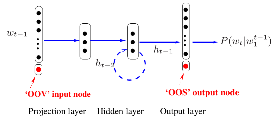
Fig. 1: An example unidirectional RNNLM.

Perplexity (PPL) is a metric used widely to evaluate the quality of language models. According to the definition in [17], the perplexity can be computed based on sentence probability with,

$${\tt PPL} = \exp\big{(}-\frac{1}{N}\sum_{j=1}^{J}\log P_{u}(\mathcal{W}_{j})\big{)}$$ (4)

$$= \exp\big{(}-\frac{1}{N}\sum_{j=1}^{J}\log P_{u}(w_{1}^{L_{j}})\big{)}$$

$$= \exp\big{(}-\frac{1}{N}\sum_{j=1}^{J}\sum_{t=1}^{L_{j}}\log P(w_{t}|w_{1}^{t-1})\big{)}$$

Where $N$ is the total number of words and $J$ is the number of sentence in the evaluation corpus. $L_{j}$ is the number of word in $j$th sentence. From the above equation, the PPL is calculated based on the average log probability of each word, which for unidirectional LMs, yields the average sentence log probability.

Uni-RNNLMs can be trained efficiently on Graphics Processing Units (GPUs) by using spliced sentence bunch (i.e. minibatch) mode [12]. Multiple sentences can be concatenated together to form a longer sequence and sets of these long sequences can then be aligned in parallel from left to right. This data structure is more efficient for minibatch based training as they have comparable sequence length [12]. When using these forms of language models for tasks like speech recognition, N-best rescoring is the most straightforward way to apply uni-RNNLMs. Lattice rescoring is also possible by introducing approximations [8] to control merging and expansion of different paths in lattice. This will be described in more detail in Section 4.

2.2 Bidirectional RNNLMs

Figure 2 illustrates an example of bidirectional RNNLMs (bi-RNNLMs). Unlike uni-RNNLMs, both the history word context $w_{1}^{t-1}$ and future word context $w_{t+1}^{L}$ are used to estimate the probability of current word $P(w_{t}|w_{1}^{t-1},w_{t+1}^{L})$. Two recurrent units are used to capture the previous and future information respectively. In the same fashion as uni-RNNLMs, $h_{t-1}$ is a compact continuous vector of the history information $w_{1}^{t-1}$. While $\tilde{h}_{t+1}$ is another continuous vector to encode the future information $w_{t+1}^{L}$. This future context vector is computed from the next word $w_{t+1}$ and the previous future context vector $\tilde{h}_{t+2}$ containing information of $w_{t+2}^{L}$. The concatenation of $h_{t-1}$ and $\tilde{h}_{t+1}$ is then fed into the output layer, with softmax function, to calculate the output probability. In order to reduce the number of parameter, the projection layer for the previous and future words are often shared.

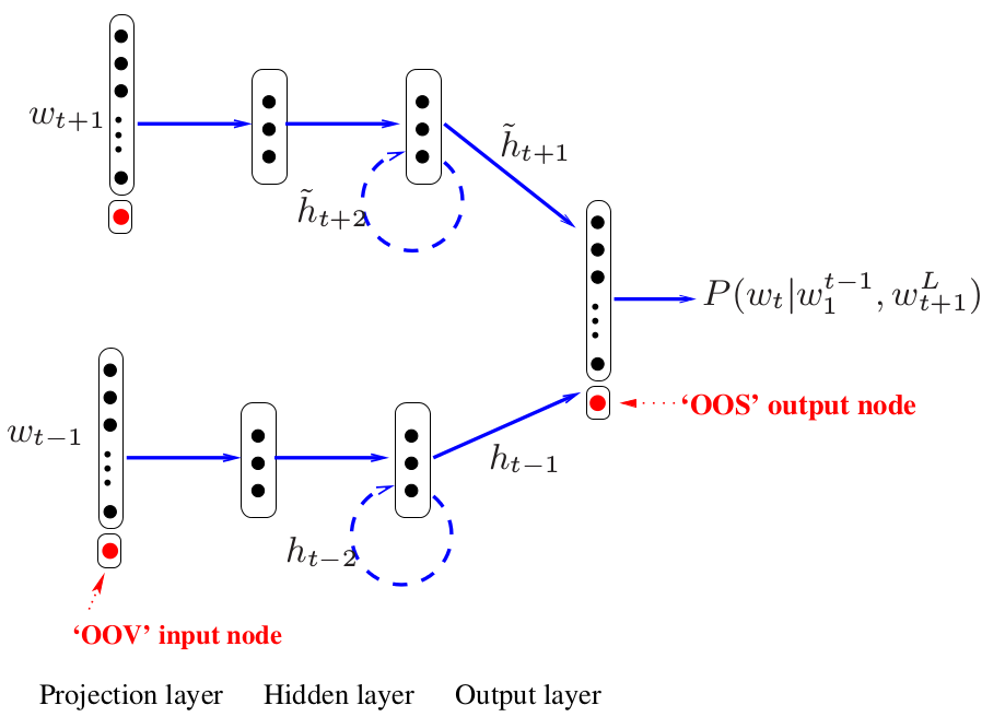
Fig. 2: An example bidirectional RNNLM.

The probability of word sequence $\mathcal{W}=w_{1}^{L}$ can be computed using bi-RNNLMs as,

$$P_{b}(w_{1}^{L})=\frac{1}{Z_{b}}\hat{P}_{b}(\mathcal{W})=\frac{1}{Z_{b}}\prod_{t=1}^{L}P(w_{t}|w_{1}^{t-1},w_{t+1}^{L})$$ (5)

$\hat{P}_{b}(\mathcal{W})$ is the unnormalized sentence probability computed from the individual word probabilities of the bi-RNNLM. $Z_{b}$ is a sentence-level normalization term to ensure the sentence probability is appropriately normalized. This is defined as,

$$Z_{b}=\sum_{\mathcal{W}\in\Theta}\hat{P}_{b}(\mathcal{W})$$ (6)

where $\Theta$ is the set of all possible sentences. Unfortunately, this normalization term is impractical to calculate for most tasks.

In a similar form to Equation 4, the PPL of bi-RNNLMs can be calculated based on sentence probability as,

$${\tt PPL} = \exp\big{(}-\frac{1}{N}\sum_{j=1}^{J}\log P_{b}(w_{1}^{L_{j}})\big{)}$$

$$= \exp\big{(}-\frac{1}{N}\sum_{j=1}^{J}\log\frac{1}{Z_{b}}\hat{P}_{b}(w_{1}^{L_{j}})\big{)}$$

$$= \exp\big{(}\frac{J}{N}\log(Z_{b})-\frac{1}{N}\sum_{j=1}^{J}\sum_{t=1}^{L_{j}}\log P(w_{t}|w_{1}^{t-1},w_{t+1}^{L_{j}})\big{)}$$

However, $Z_{b}$ is often infeasible to obtain. As a result, it is not possible to compute a valid perplexity from bi-RNNLMs. Nevertheless, the average log probability of each word can be used to get a “pseudo” perplexity (PPL).

$${\tt PPL_{pseudo}}=\exp\big{(}-\frac{1}{N}\sum_{j=1}^{J}\sum_{t=1}^{L_{j}}\log P(w_{t}|w_{1}^{t-1},w_{t+1}^{L_{j}})\big{)}$$ (8)

This is the second term of the valid PPL of bi-RNNLMs shown in Equation 2.2. It is a “pseudo” PPL because the normalized sentence probability ${P}_{b}(\mathcal{W})$ is impossible to obtain and the unnormalized sentence probability $\hat{P}_{b}(\mathcal{W})$ is used instead. Hence, the “pseudo” PPL of bi-RNNLMs is not comparable with the valid PPL of uni-RNNLMs. However, the value of “pseudo” PPL provides information on the average word probability from bi-RNNLMs since it is obtained using the word probability.

In order to achieve good performance for speech recognition, [7] proposed an additional smoothing of the bi-RNNLM probability at test time. The probability of bi-RNNLMs is smoothed as,

$$P(w_{i}|w_{1}^{t-1},w_{t+1}^{L})=\frac{\exp(\alpha y_{i})}{\sum_{j}^{\mathcal{V}}\exp(\alpha y_{j})}$$ (9)

where $y_{i}$ is the activation before softmax function for node $i$ in the output layer. $\alpha$ is an empirical smoothing factor, which is chosen as 0.7 in this paper.

The use of both preceding and following context information in bi-RNNLMs presents challenges to both model training and inference. First, N-best rescoring is normally used for speech recognition [7]. Lattice rescoring is impractical for bi-RNNLMs as the computation of word probabilities requires information from the complete sentence.

Another drawback of bi-RNNLMs is the difficulty in training. The complete previous and future context information is required to predict the probability of each word. It is expensive to directly training bi-RNNLMs sentence by sentence, and difficult to parallelise the training for efficiency. In [6], all sentences in the training corpus were concatenated together to form a single sequence to facilitate minibatch based training. This sequence was then “chopped” into sub-sequences with the average sentence length. Bi-RNNLMs were then trained on GPU by processing multiple sequences at the same time. This allows bi-RNNLMs to be efficiently trained. However, issues can arise from the random cutting of sentences, history and future context vectors may be reset in the middle of a sentence. In [7], the bi-RNNLMs were trained in a more consistent fashion. Multiple sentences were aligned from left to right to form minibatches during bi-RNNLM training. In order to handle issues caused by variable sentence length, NULL tokens were appended to the ends of sentences to ensure that the aligned sentences had the same length. These NULL tokens were not used for parameter update. In this paper, this approach is adopted to train bi-RNNLMs as it gave better performance.

3 RNNLMs with succeeding words

As discussed above, bi-RNNLMs are slow to train and difficult to use in lattice rescoring. In order to address these issues, a novel structure, the su-RNNLM, is proposed in this paper to incorporate future context information. The model structure is illustrated in Figure 3. In the same fashion as bi-RNNLMs, the previous history $w_{1}^{t-1}$ is modeled with recurrent units (e.g. LSTM, GRU). However, instead of modeling the complete future context information, $w_{t+1}^{L}$, using recurrent units, feedforward units are used to capture a finite number of succeeding words, $w_{t+1}^{t+k}$. The softmax function is again applied at the output layer to obtain the probability of the current word $P(w_{t}|w_{1}^{t-1},w_{t+1}^{t+k})$. The word embedding in the projection layer are shared for all input words. When the succeeding words are beyond the sentence boundary, a vector of 0 is used as the word embedding vector. This is similar to the zero padding of the feedforward forward NNLMs at the beginning of each sentence [13].

As the number of succeeding words is finite and fixed for each word, its succeeding words can be organized as a $n$-gram future context and used for minibatch mode training as in feedforward NNLMs [13]. Su-RNNLMs can then be trained efficiently in a similar fashion to uni-RNNLMs in a spliced sentence bunch mode [12].

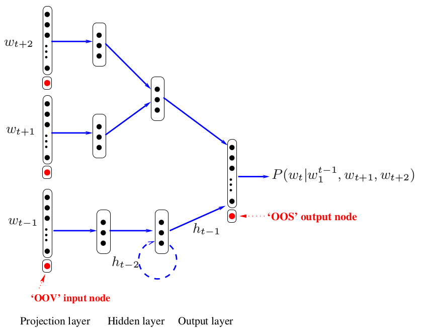
Fig. 3: An example su-RNNLM with 2 succeeding words.

Compared with equations 3 and 5, the probability of word sequence $w_{1}^{L}$ can be computed as

$$P_{s}(w_{1}^{L})=\frac{1}{Z_{s}}\prod_{t=1}^{L}P(w_{t}|w_{1}^{t-1},w_{t+1}^{t+k})$$ (10)

Again, the sentence level normalization term $Z_{s}$ is difficult to compute and only “pseudo” PPL can be obtained. The probabilities of su-RNNLMs are also very sharp, which can be seen from the “pseudo” PPLs in Table 2 in Section 6. Hence, the bi-RNNLM probability smoothing given in Equation 9 is also required for su-RNNLMs to achieve good performance at evaluation time.

4 Lattice rescoring

Lattice rescoring with feedforward NNLMs is straightforward [13] whereas approximations are required for uni-RNNLMs lattice rescoring [8, 18]. As mentioned in Section 2.2, N-best rescoring has previously been used for bi-RNNLMs. It is not practical for bi-RNNLMs to be used for lattice rescoring and generation as both the complete previous and future context information are required. However, lattices are very useful in many applications, such as confidence score estimation [9], keyword search [10] and confusion network decoding [11]. In contrast, su-RNNLMs require a fixed number of succeeding words, instead of the complete future context information. From Figure 3, su-RNNLMs can be viewed as a combination of uni-RNNLMs for history information and feedforward NNLMs for future context information. Hence, lattice rescoring is feasible for su-RNNLMs by extending the lattice rescoring algorithm of uni-RNNLMs by considering additional fixed length future contexts.

4.1 Lattice rescoring of uni-RNNLMs

In this paper, the $n$-gram approximation [8] based approach is used for uni-RNNLMs lattice rescoring. When considering merging of two paths, if their previous $n-1$ words are identical, the two paths are viewed as “equivalent” and can be merged. This is illustrated in Figure 5 for the start node of word $w_{4}$. The history information from the best path is kept for the following RNNLM probability computation and the histories of all other paths are discarded. For example, the path $(w_{0},w_{2},w_{3})$ is kept and the other path $(w_{1},w_{2},w_{3})$ is discarded given arc $w_{4}$.

There are two types of approximation involved for uni-RNNLM lattice rescoring, which are the merge and cache approximations. The merge approximation controls the merging of two paths. In [8], the first path reaching the node was kept and all other paths with the same $n$-gram history were discarded irrespective of the associated scores. This introduces inaccuracies in the RNNLM probability calculation. The merge approximation can be improved by keeping the path with the highest accumulated score. This is the approach adopted in this work. For fast probability lookup in lattice rescoring, $n$-gram probabilities can be cached using $n-1$ words as a key. A similar approach can be used with RNNLM probabilities. In [8], RNNLM probabilities were cached based on the previous $n-1$ words, which is referred as cache approximation. Thus a word probability obtained from the cache may be derived from another history sharing the same $n-1$ previous words. This introduces another inaccuracy. In order to avoid this inaccuracy yet maintain the efficiency, the cache approximation used in [8] is improved by adopting the complete history as key for caching RNNLM probabilities. Both modifications yielt small but consistent improvements over [8] on a range of tasks.

4.2 Lattice rescoring of su-RNNLMs

For lattice rescoring with su-RNNLMs, the $n$-gram approximation can be adopted and extended to support the future word context. In order to handle succeeding words correctly, paths will be merged only if the following succeeding words are identical. In this way, the path expansion is carried out in both directions. Any two paths with the same succeeding words and $n-1$ previous words are merged.

Figure 4 shows part of an example lattice generated by a 2-gram LM. In order to apply uni-RNNLM lattice rescoring using a 3-gram approximation, the grey shaded node in Figure 4 needs to be duplicated as word $w_{3}$ has two distinct 3-gram histories, which are $(w_{0},w_{2})$ and $(w_{1},w_{2})$ respectively. Figure 5 shows the lattice after rescoring using a uni-RNNLM with 3-gram approximation. In order to apply su-RNNLMs for lattice rescoring, the succeeding words also need to be taken into account. Figure 6 is the expanded lattice using a su-RNNLM with 1 succeeding word. The grey shaded nodes in Figure 5 need to be expanded further as they have distinct succeeding words. The blue shaded nodes in Figure 6 are the expanded node in the resulting lattice.

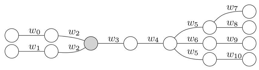
Fig. 4: Lattice generated by 2-gram LM.

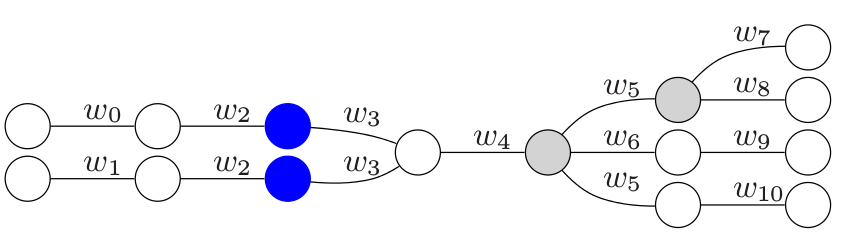
Fig. 5: Lattice generated by uni-RNNLMs with 3-gram approximation.

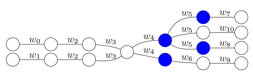
Fig. 6: Lattice generated by su-RNNLMs with 3-gram approximation for history context and 1 succeeding word.

Using the $n$-gram history approximation and given $k$ succeeding words, the lattice expansion process is effectively a $n+k$-gram lattice expansion for uni-RNNLMs. For larger value of $n$ and $k$, the resulting lattices can be very large. This can be addressed by pruning the lattice and doing initial lattice expansion with a uni-RNNLM.

5 Language Model Interpolation

For unidirectional language models, such as $n$-gram model and uni-RNNLMs, the word probabilities are normally combined using linear interpolation,

$$P_{u}(w_{t}|w_{1}^{t-1})=$$

$$(1-\lambda_{1})P_{n}(w_{t}|w_{1}^{t-1})+\lambda_{1}P_{r}(w_{t}|w_{1}^{t-1})$$

where $P_{n}$ and $P_{r}$ are the probabilities from $n$-gram and uni-RNN LMs respectively, $\lambda_{1}$ is the interpolation weight of uni-RNNLMs.

However, it is not valid to directly combine uni-LMs (e.g unidirectional $n$-gram LMs or RNNLMs) and bi-LMs (or su-LMs) using linear interpolation due to the sentence level normalisation term required for bi-LMs (or su-LMs) in Equation 5. As described in [7], uni-LMs can be log-linearly interpolated with bi-LMs for speech recognition using,

$$P(w_{t}|w_{1}^{t-1},w_{t+1}^{L})=$$

$$\frac{1}{Z}P_{u}(w_{t}|w_{1}^{t-1})^{(1-\lambda_{2})}P_{b}(w_{t}|w_{1}^{t-1},w_{t+1}^{L})^{\lambda_{2}}$$

where $Z$ is the appropriate normalisation term. The normalisation term can be discarded for speech recognition as it does not affect the hypothesis ranking. $P_{u}$ and $P_{b}$ are the probabilities from uni-LMs and bi-RNNLMs respectively. $\lambda_{2}$ is the log-linear interpolation weight of bi-RNNLMs. The issue of normalisation term in su-RNLMs is similar to that of bi-RNNLMs, as shown in Equation 10. Hence, log-linear interpolation can also be applied for the combination of su-RNNLMs and uni-LMs and is the approach used in this paper.

By default, linear interpolation is used to combine uni-RNNLMs and $n$-gram LMs. A two-stage interpolation is used when including bi-RNNLMs and su-RNNLMs. The uni-RNNLMs and $n$-gram LMs are first interpolated using linear interpolation. These linearly interpolated probabilities are then log-linearly interpolated with those of bi-RNNLMs (or su-RNNLMs).

6 Experiments

Experiments were conducted using the AMI IHM meeting corpus [19] to evaluated the speech recognition performance of various language models. The Kaldi training data configuration was used. A total of 78 hours of speech was used in acoustic model training. This consists of about 1M words of acoustic transcription. Eight meetings were excluded from the training set and used as the development and test sets.

The Kaldi acoustic model training recipe [20] featuring sequence training [21] was applied for deep neural network (DNN) training. CMLLR transformed MFCC features [22] were used as the input and 4000 clustered context dependent states were used as targets. The DNN was trained with 6 hidden layers, and each layer has 2048 hidden nodes.

The first part of the Fisher corpus, 13M words, was used for additional language modeling training data. A 49k word decoding vocabulary was used for all experiments. All LMs were trained on the combined (AMI+Fisher), 14M word in total. A 4-gram KN smoothed back-off LM without pruning was trained and used for lattices generation. GRU based recurrent units were used for all unidirectional and bidirectional RNNLMs . 512 hidden nodes were used in the hidden layer. An extended version of CUED-RNNLM [23] was developed for the training of uni-RNNLMs, bi-RNNLMs and su-RNNLMs. The related code and recipe will be available online . The linear interpolation weight $\lambda_{1}$ between 4-gram LMs and uni-RNNLMs was set to be 0.75 as it gave the best performance on the development data. The log-linear interpolation weight $\lambda_{2}$ for bi-RNNLMs (or su-RNNLMs) was 0.3. The probabilities of bi-RNNLMs and su-RNNLMs were smoothed with a smoothing factor 0.7 as suggested in [7]. The 3-gram approximation was applied for the history merging of uni-RNNLMs and su-RNNLMs during lattice rescoring and generation [8].

Table 1 shows the word error rates of the baseline system with 4-gram and uni-RNN LMs. Lattice rescoring and $100$-best rescoring are applied to lattices generated by the 4-gram LM. As expected, uni-RNNLMs yield a significant performance improvement over 4-gram LMs. Lattice rescoring gives a comparable performance with 100-best rescoring. Confusion network (CN) decoding can be applied to lattices generated by uni-RNNLM lattice rescoring and additional performance improvements can be achieved. However, it is difficult to apply confusion network decoding to the 100-best .

LM	rescore	dev		eval
		Vit	CN	Vit	CN
ng4	-	23.8	23.5	24.2	23.9
+uni-rnn	100-best	21.7	-	22.1	-
	lattice	21.7	21.5	21.9	21.7

Table 1: Baseline WER results on AMI corpus

Table 2 gives the training speed measured with word per second (w/s) and (“pseudo”) PPLs of various RNNLMs with difference amounts of future word context. When the number of succeeding words is 0, this is the baseline uni-RNNLMs. When the number of succeeding words is set to $\infty$, a bi-RNNLM with complete future context information is used. It can be seen that su-RNNLMs give a comparable training speed as uni-RNNLMs. The additional computational load of the su-RNNLMs mainly come from the feedforward unit for succeeding words as shown in Figure 3. The computation in this part is much less than that of other parts such as output layer and GRU layers. However, the training of su-RNNLMs is much faster than bi-RNNLMs as it is difficult to parallelise the training of bi-RNNLMs efficiently [7]. It is worth mentioning again that the PPLs of uni-RNNLMs can not be compared directly with the “pseudo” PPLs of bi-RNNLMs and su-RNNLMs. But both PPLs and “pseudo” PPLs reflect the average log probability of each word. From Table 2, with increasing number of succeeding words, the “pseudo” PPLs of the su-RNNLMs keeps decreasing, yielding comparable value as bi-RNNLMs.

#succ words	0	1	3	7	$\infty$
train speed(w/s)	4.5K	4.5K	3.9K	3.8K	0.8K
(pseudo) PPL	66.8	25.5	21.5	21.3	22.4

Table 2: Train speed and (Pseudo) Perplexity of uni-, bi-, and su-RNNLMs. 0 succeeding word is for uni-RNNLMs and $\infty$ for bi-RNNLMs.

Table 3 gives the WER results of 100-best rescoring with various language models. For bi-RNNLMs (or su-RNNLMs), it is not possible to use linear interpolation. Thus a two stage approach is adopted as described in Section 5. This results in slight differences, second decimal place, between the uni-RNNLM case and the 0 future context su-RNNLM. The increasing number of the succeeding words consistently reduces the WER. With 1 succeeding word, the WERs were reduced by 0.2% absolutely. Su-RNNLMs with more than 2 succeeding words gave about 0.5% absolute WER reduction. Bi-RNNLMs (shown in the bottom line of Table 3) outperform su-RNNLMs by 0.1% to 0.2%, as it is able to incorporate the complete future context information with recurrent connection.

LM	#succ words	dev	eval
ng4		23.8	24.2
+uni-rnn	-	21.7	22.1
+su-rnn	0	21.7	22.1
	1	21.5	21.8
	2	21.3	21.7
	3	21.3	21.6
	4	21.4	21.6
	5	21.3	21.6
	6	21.3	21.6
	7	21.4	21.6
	$\infty$	21.2	21.4

Table 3: WERs of uni-, bi, and su-RNNLMs with 100-best rescoring. 0 succeeding word is for uni-RNNLMs and $\infty$ for bi-RNNLMs.

Table 4 shows the WERs of lattice rescoring using su-RNNLMs. The lattice rescoring algorithm described in Section 4 was applied. Su-RNNLMs with 1 and 3 succeeding words were used for lattice rescoring. From Table 4, su-RNNLMs with 1 succeeding words give 0.2% WER reduction and using 3 succeeding words gives about 0.5% WER reduction. These results are consistent with the 100-best rescoring result in Table 3. Confusion network decoding can be applied on the rescored lattices and additional 0.3-0.4% WER performance improvements are obtained on dev and eval test sets.

LM	#succ	dev		eval
	words	Vit	CN	Vit	CN
ng4	-	23.8	23.5	24.2	23.9
+uni-rnn	-	21.7	21.5	21.9	21.7
+su-rnn	1	21.6	21.3	21.6	21.5
	3	21.3	21.0	21.4	21.1

Table 4: WERs of uni-RNNLMs and su-RNNLMs with lattice rescoring

7 Conclusions

In this paper, the use of future context information on neural network language models has been explored. A novel model structure is proposed to address the issues associated with bi-RNNLMs, such as slow train speed and difficulties in lattice rescoring. Instead of using a recurrent unit to capture the complete future information, a feedforward unit was used to model a finite number of succeeding words. The existing training and lattice rescoring algorithms for uni-RNNLMs are extended for the proposed su-RNNLMs. Experimental results show that su-RNNLMs achieved a slightly worse performances than bi-RNNLMs, but with much faster training speed. Furthermore, additional performance improvements can be obtained from lattice rescoring and subsequent confusion network decoding. Future work will examine improved pruning scheme to address the lattice expansion issues associated with larger future context.

References

- [1] Stanley Chen and Joshua Goodman, “An empirical study of smoothing techniques for language modeling,” Computer Speech & Language, vol. 13, no. 4, pp. 359–393, 1999.
- [2] Yoshua Bengio, Réjean Ducharme, Pascal Vincent, and Christian Jauvin, “A neural probabilistic language model,” Journal of Machine Learning Research, vol. 3, pp. 1137–1155, 2003.
- [3] Tomas Mikolov, Martin Karafiát, Lukas Burget, Jan Cernockỳ, and Sanjeev Khudanpur, “Recurrent neural network based language model.,” in Proc. ISCA INTERSPEECH, 2010.
- [4] Wayne Xiong, Jasha Droppo, Xuedong Huang, Frank Seide, Mike Seltzer, Andreas Stolcke, Dong Yu, and Geoffrey Zweig, “Achieving human parity in conversational speech recognition,” arXiv preprint arXiv:1610.05256, 2016.
- [5] Yangyang Shi, Martha Larson, Pascal Wiggers, and Catholijn Jonker, “Exploiting the succeeding words in recurrent neural network language models.,” in Proc. ICSA INTERSPEECH, 2013.
- [6] Ebru Arisoy, Abhinav Sethy, Bhuvana Ramabhadran, and Stanley Chen, “Bidirectional recurrent neural network language models for automatic speech recognition,” in Proc. ICASSP. IEEE, 2015, pp. 5421–5425.
- [7] Xie Chen, Anton Ragni, Xunying Liu, and Mark Gales, “Investigating bidirectional recurrent neural network language models for speech recognition.,” in Proc. ICSA INTERSPEECH, 2017.
- [8] Xunying Liu, Xie Chen, Yongqiang Wang, Mark Gales, and Phil Woodland, “Two efficient lattice rescoring methods using recurrent neural network language models,” IEEE/ACM Transactions on Audio, Speech, and Language Processing, vol. 24, no. 8, pp. 1438–1449, 2016.
- [9] Frank Wessel, Ralf Schluter, Klaus Macherey, and Hermann Ney, “Confidence measures for large vocabulary continuous speech recognition,” Speech and Audio Processing, IEEE Transactions on, vol. 9, no. 3, pp. 288–298, 2001.
- [10] Xie Chen, Anton Ragni, Jake Vasilakes, Xunying Liu, Kate Knill, and Mark Gales, “Recurrent neural network language models for keyword search,” in Proc. ICASSP. IEEE, 2017, pp. 5775–5779.
- [11] Lidia Mangu, Eric Brill, and Andreas Stolcke, “Finding consensus in speech recognition: word error minimization and other applications of confusion networks,” Computer Speech & Language, vol. 14, no. 4, pp. 373–400, 2000.
- [12] Xie Chen, Xunying Liu, Yongqiang Wang, Mark Gales, and Phil Woodland, “Efficient training and evaluation of recurrent neural network language models for automatic speech recognition,” IEEE/ACM Transactions on Audio, Speech, and Language Processing, 2016.
- [13] Holger Schwenk, “Continuous space language models,” Computer Speech & Language, vol. 21, no. 3, pp. 492–518, 2007.
- [14] Junyoung Chung, Caglar Gulcehre, KyungHyun Cho, and Yoshua Bengio, “Empirical evaluation of gated recurrent neural networks on sequence modeling,” arXiv preprint arXiv:1412.3555, 2014.
- [15] Sepp Hochreiter and Jürgen Schmidhuber, “Long short-term memory,” Neural computation, vol. 9, no. 8, pp. 1735–1780, 1997.
- [16] Junho Park, Xunying Liu, Mark Gales, and Phil Woodland, “Improved neural network based language modelling and adaptation,” in Proc. ISCA INTERSPEECH, 2010.
- [17] Frederick Jelinek, “The dawn of statistical asr and mt,” Computational Linguistics, vol. 35, no. 4, pp. 483–494, 2009.
- [18] Martin Sundermeyer, Hermann Ney, and Ralf Schluter, “From feedforward to recurrent lstm neural networks for language modeling,” Audio, Speech, and Language Processing, IEEE/ACM Transactions on, vol. 23, no. 3, pp. 517–529, 2015.
- [19] Jean Carletta et al., “The AMI meeting corpus: A pre-announcement,” in Machine learning for multimodal interaction, pp. 28–39. Springer, 2006.
- [20] Daniel Povey, Arnab Ghoshal, Gilles Boulianne, Lukas Burget, Ondrej Glembek, Nagendra Goel, Mirko Hannemann, Petr Motlicek, Yanmin Qian, Petr Schwarz, et al., “The Kaldi speech recognition toolkit,” in ASRU, IEEE Workshop on, 2011.
- [21] Karel Veselỳ, Arnab Ghoshal, Lukás Burget, and Daniel Povey, “Sequence-discriminative training of deep neural networks.,” in Proc. ICSA INTERSPEECH, 2013.
- [22] Mark Gales, “Maximum likelihood linear transformations for HMM-based speech recognition,” Computer Speech & Language, vol. 12, no. 2, pp. 75–98, 1998.
- [23] Xie Chen, Xunying Liu, Mark Gales, and Phil Woodland, “CUED-RNNLM – an open-source toolkit for efficient training and evaluation of recurrent neural network language models,” in Proc. ICASSP. IEEE, 2015.