Measuring properties of a Heavy Higgs boson
in the $H\to ZZ\to 4\ell$ decay

Abstract

In many extensions of the standard model, there exist a few extra Higgs bosons. Suppose a heavy neutral Higgs boson $H$ is discovered at the LHC, one could then investigate CP and CP$\widetilde{\rm T}$ properties of its couplings to a pair of $Z$ bosons through $H\to ZZ\to 4\ell$. We use the helicity-amplitude method to write down the most general form for the angular distributions of the four final-state leptons, which can cover the case of CP-even, -odd, and -mixed state for the Higgs boson. We figure out there are 9 types of angular observables and all the $H$ couplings to $Z$ bosons can be fully determined by exploiting them. A Higgs-boson mass of 260 GeV below the $t\bar{t}$ threshold is illustrated with full details. With a total of $10^{3}$ events of $H\to ZZ\to 4\ell$, one can determine the couplings up to 12-20% uncertainties.

I Introduction

The measured properties of the scalar boson which was discovered at the LHC atlas ; cms turn out to be the best described by the Standard Model (SM) Higgs boson Cheung:2013kla and it deserves to be called the Higgs boson which was proposed in 1960s higgs . Among the Higgs boson couplings to the SM particles, the most constrained one is its coupling to the massive gauge bosons normalized to the corresponding SM value: $C_{v}=0.94\,^{+0.11}_{-0.12}$.

Even though the SM has achieved a great success in describing the interactions among the basic building blocks of matter scrutinized by now, however more blocks and new interactions are required to explain the experimental observations of dark matter, non-vanishing neutrino mass, the baryon asymmetry of our Universe, inflation, etc. In most extensions beyond the SM, the Higgs sector is enlarged to include more than one Higgs doublet resulting in charged Higgs bosons and several neutral Higgs bosons in addition to the one discovered at the LHC. For example, the minimal supersymmetric extension of the SM, aka MSSM HPN , requires two Higgs doublet fields, thus leading to a pair of charged Higgs bosons and 3 neutral ones. In the next-to-minimal supersymmetric standard model, there are two additional neutral Higgs bosons Cheung:2010ba . As another example, the Higgs Triplet Model that can explain the mass spectrum and mixing of neutrinos gives rise to a pair of doubly-charged Higgs bosons, a pair of singly-charged Higgs bosons, and 3 neutral ones Akeroyd:2005gt .

Suppose that in future experiments a neutral Higgs boson $H$ heavier than the SM 125 GeV Higgs boson (denoted by $h$) is discovered. Below the decay threshold into a top-quark pair or when $M_{H}<2m_{t}$, assuming $H$ does not carry any definite CP-parity, it may mainly decay into a bottom-quark pair ($b\bar{b}$), tau leptons ($\tau^{+}\tau^{-}$), massive vector bosons ($W^{+}W^{-}$ and $ZZ$), a pair of $125$ GeV Higgs bosons ($hh$), and a massive gauge boson and a lighter Higgs boson ($hZ$). Above the $2m_{t}$ threshold, the decay mode into a top-quark pair may dominate as in the MSSM .

The fermionic decay modes of $H\to b\bar{b},\tau^{+}\tau^{-},t\bar{t}$ and one of the bosonic decay modes $H\to W^{+}W^{-}$ may suffer from large QCD backgrounds and/or missing neutrinos. Among the remaining bosonic decay modes into $ZZ$, $hh$, and $hZ$, taking account of the spin-$0$ nature of $H$, only the $ZZ$ mode may lead to nontrivial angular correlations among the decay products of the $Z$ bosons through the interferences among various helicity states of the two intermediate $Z$ bosons before their decays.

In this work, we consider the decay $H\to ZZ$ with the $Z$ bosons subsequently decaying into electrons and/or muons: $H\to ZZ\to 4\ell$. Long before the discovery of the SM Higgs boson, it was suggested to exploit this decay process to determine the spin and parity of the Higgs boson Choi:2002jk . Later, more rigorous angular analyses of spin-zero, -one, and -two resonances were illustrated with certain levels of experimental simulations Gao:2010qx . After the 125 GeV Higgs-boson discovery, the method was practically applied to determine the spin and CP properties of the “newly” discovered boson Bolognesi:2012mm ; Modak:2013sb . Here, we shift the focus from the SM Higgs to a heavy Higgs boson $H$ , and pursue complete determination of its couplings from the angular correlations among the charged leptons in the final state. Under the current experimental status, in which active searches for heavy resonances decaying into a $ZZ$ pair have been continually performed h_zz , our study may show how well one can determine the properties of such a heavy scalar Higgs boson at the LHC and/or High Luminosity LHC (HL-LHC).

The remainder of this article is organized as follows. In Sec. II, based on the helicity amplitude method Hagiwara:1985yu , we present a formalism for the study of angular distributions in the decay $H\to ZZ\to 4\ell$. We point out that there can be 9 angular observables in general and we can classify them according to the CP and CP$\widetilde{\rm T}$ parities of each observable. In Sec. III, we illustrate how well one can measure the couplings of a heavy Higgs boson by exploiting the angular observables introduced in Sec. II. Finally, Sec. IV is devoted to a brief summary, some prospects for future work and conclusions.

II Formalism

One may start by defining the interaction of the heavy Higgs boson $H$ with a pair of $Z$ bosons. The amplitude for the decay process $H\to Z(k_{1},\epsilon_{1})\ Z(k_{2},\epsilon_{2})$ can be written as

$$i{\cal M}^{H\to ZZ} \equiv i\frac{gM_{W}}{c_{W}^{2}}\ \Gamma^{ZZ}_{\mu\nu}\epsilon_{1}^{*\mu}\epsilon_{2}^{*\nu}$$ (1)

$$= i\frac{gM_{W}}{c_{W}^{2}}\Bigg{\{}g_{{}_{HZZ}}\,\epsilon_{1}^{*}\cdot\epsilon_{2}^{*}+S^{ZZ}_{H}(s)\left[\frac{-2k_{1}\cdot k_{2}}{s}\,\epsilon_{1}^{*}\cdot\epsilon_{2}^{*}\ +\ \frac{2}{s}\,k_{1}\cdot\epsilon_{2}^{*}\,k_{2}\cdot\epsilon_{1}^{*}\right]$$

$$\hskip 97.02399pt+\ P^{ZZ}_{H}(s)\,\frac{2}{s}\,\langle\epsilon_{1}^{*}\epsilon_{2}^{*}k_{1}k_{2}\rangle\Bigg{\}}$$

where $k_{1,2}$ and $\epsilon_{1,2}$ are the four-momenta and the wave vectors of the two $Z$ bosons, respectively, with $s=(k_{1}+k_{2})^{2}=M_{H}^{2}$ and $\langle\epsilon_{1}^{*}\epsilon_{2}^{*}k_{1}k_{2}\rangle\equiv\epsilon_{\mu\nu\rho\sigma}\epsilon_{1}^{*\mu}\epsilon_{2}^{*\nu}k_{1}^{\rho}k_{2}^{\sigma}$. The first term may come from the dimension-four renormalizable operator

$${\cal L}=\frac{gM_{W}}{2c_{W}^{2}}\ g_{{}_{HZZ}}\ Z_{\mu}Z^{\mu}H$$ (2)

while the form factors $S^{ZZ}_{H}$ and $P^{ZZ}_{H}$ can be generated by including higher-order corrections and/or introducing non-renormalizable operators. In the former case, $S^{ZZ}_{H}$ and $P^{ZZ}_{H}$ can be complex by developing non-vanishing absorptive parts in the existence of (New Physics) particles running in the loop with mass less than $M_{H}/2$. Therefore, in general one may need 5 real parameters to describe the interaction of the heavy Higgs boson $H$ with a pair of $Z$ bosons. Note that $g_{{}_{HZZ}}^{2}\leq 1-g_{{}_{hZZ}}^{2}=1-C_{v}^{2}$ with equality holding when $h$ and $H$ are the only Higgs bosons participating in the electroweak-symmetry breaking. We observe that being different from the case of SM Higgs boson, in which $g_{{}_{hZZ}}$ is dominating over the loop-induced $S_{h}^{ZZ}$ and $P_{h}^{ZZ}$ couplings, each of the couplings $g_{{}_{HZZ}}$, $S_{H}^{ZZ}$, and $P_{H}^{ZZ}$ may contribute comparably in the heavy Higgs-boson case. We further observe that either $g_{{}_{HZZ}}\times P_{H}^{ZZ}\neq 0$ or $S_{H}^{ZZ}\times P_{H}^{ZZ}\neq 0$ implies that $H$ is a CP-mixed state, thus signaling CP violation.

Incidentally, the interaction of the $Z$ boson with a fermion pair is described by the interaction Lagrangian:

$${\cal L}_{Zff}=-\frac{g}{c_{W}}\ \bar{f}\gamma_{\mu}(v_{f}-a_{f}\gamma_{5})f\ Z^{\mu}=-\frac{g}{c_{W}}\ \sum_{A=+(R),-(L)}\bar{f}\gamma_{\mu}(v_{f}-Aa_{f})P_{A}f\ Z^{\mu}$$ (3)

with $v_{f}=I_{3}^{f}/2-Q_{f}s_{W}^{2}$, $a_{f}=I_{3}^{f}/2$ and $P_{A}=(1+A\gamma_{5})/2$.

II.1 Helicity amplitude

We first present the helicity amplitude for the process $H\ \to Z(k_{1},\epsilon_{1})Z(k_{2},\epsilon_{2})\to f_{1}(p_{1},\sigma_{1})\bar{f}_{1}(\bar{p}_{1},\bar{\sigma}_{1})\ f_{2}(p_{2},\sigma_{2})\bar{f}_{2}(\bar{p}_{2},\bar{\sigma}_{2})$. Here, $p_{1,2}$ and and $\bar{p}_{1,2}$ are four-momenta of the fermions $f_{1,2}$ and $\bar{f}_{1,2}$, respectively, with $k_{1,2}=p_{1,2}+\bar{p}_{1,2}$. And we denote the helicities of $f_{1,2}$ and $\bar{f}_{1,2}$ by $\sigma_{1,2}$ and $\bar{\sigma}_{1,2}$. Depending on the helicities of the four final-state fermions, the amplitude can be cast into the form

$$i{\cal M}_{\sigma_{1}\bar{\sigma}_{1}:\sigma_{2}\bar{\sigma}_{2}} = \left(i\frac{gM_{W}}{c_{W}^{2}}\Gamma^{ZZ}_{\mu\nu}\right)\ \frac{-i\left(g^{\mu\rho}-\frac{k_{1}^{\mu}k_{1}^{\rho}}{M_{Z}^{2}}\right)}{k_{1}^{2}-M_{Z}^{2}+iM_{Z}\Gamma_{Z}}\ \frac{-i\left(g^{\nu\sigma}-\frac{k_{2}^{\nu}k_{2}^{\sigma}}{M_{Z}^{2}}\right)}{k_{2}^{2}-M_{Z}^{2}+iM_{Z}\Gamma_{Z}}$$

$$\times \left[-i\frac{g}{c_{W}}\ \sum_{A=L,R}\bar{u}(p_{1},\sigma_{1})\gamma_{\rho}(v_{f_{1}}-Aa_{f_{1}})P_{A}v(\bar{p}_{1},\bar{\sigma}_{1})\right]$$

$$\times \left[-i\frac{g}{c_{W}}\ \sum_{B=L,R}\bar{u}(p_{2},\sigma_{2})\gamma_{\sigma}(v_{f_{2}}-Ba_{f_{2}})P_{B}v(\bar{p}_{2},\bar{\sigma}_{2})\right]$$

$$= i\sum_{\lambda_{1},\lambda_{2}}{\cal M}^{H\to ZZ}_{\lambda_{1}\lambda_{2}}\ \frac{1}{k_{1}^{2}-M_{Z}^{2}+iM_{Z}\Gamma_{Z}}\ \frac{1}{k_{2}^{2}-M_{Z}^{2}+iM_{Z}\Gamma_{Z}}\ {\cal M}^{Z\to f_{1}\bar{f}_{1}}_{\lambda_{1}:\sigma_{1}\bar{\sigma}_{1}}{\cal M}^{Z\to f_{2}\bar{f}_{2}}_{\lambda_{2}:\sigma_{2}\bar{\sigma}_{2}}$$

using

$$-g_{\mu\nu}+\frac{k_{\mu}k_{\nu}}{m^{2}}=\sum_{\lambda=\pm,0}\epsilon_{\mu}^{*}(k,\lambda)\epsilon_{\nu}(k,\lambda)\,.$$ (5)

The helicity amplitude for the decay $H\ \to Z(k_{1},\epsilon_{1})Z(k_{2},\epsilon_{2})$ in the rest frame of $H$ is given by

$${\cal M}^{H\to ZZ}_{\lambda_{1}\lambda_{2}}=\frac{gM_{W}}{c_{W}^{2}}\,\langle\lambda_{1}\rangle\ \delta_{\lambda_{1}\lambda_{2}}$$ (6)

with the reduced amplitudes $\langle\lambda_{1}\rangle$ defined by

$$\langle+\rangle \equiv -g_{{}_{HZZ}}+(1-\alpha_{1}-\alpha_{2})\,S^{ZZ}_{H}\ -i\lambda^{1/2}(1,\alpha_{1},\alpha_{2})\,P^{ZZ}_{H}\,,$$

$$\langle-\rangle \equiv -g_{{}_{HZZ}}+(1-\alpha_{1}-\alpha_{2})\,S^{ZZ}_{H}\ +i\lambda^{1/2}(1,\alpha_{1},\alpha_{2})\,P^{ZZ}_{H}\,,$$

$$\langle 0\rangle \equiv g_{{}_{HZZ}}\left(\frac{1-\alpha_{1}-\alpha_{2}}{2\sqrt{\alpha_{1}\alpha_{2}}}\right)-2\sqrt{\alpha_{1}\alpha_{2}}\,S^{ZZ}_{H}\,,$$ (7)

where $\lambda(x,y,z)=x^{2}+y^{2}+z^{2}-2xy-2yz-2zx$ and $\alpha_{i}=k_{i}^{2}/M_{H}^{2}$. We note that the contribution of $g_{{}_{HZZ}}$ to the longitudinal amplitude $\langle 0\rangle$ is enhanced by a factor $M_{H}^{2}/2M_{Z}^{2}$ in the large $M_{H}$ limit.

On the other hand, the helicity amplitude for the decay $Z(k,\epsilon(k,\lambda))\to f(p,\sigma)\bar{f}(\bar{p},\bar{\sigma})$ is given by

$${\cal M}^{Z\to f\bar{f}}_{\lambda:\sigma\bar{\sigma}}=\left\{\begin{array}[]{ll}-\frac{g}{c_{W}}\left[\sqrt{2}m_{f}v_{f}\ \lambda\sigma e^{-i(\sigma-\lambda)\phi}\ s_{\theta}\ \delta_{\sigma\bar{\sigma}}\right.&\\[11.38109pt] \left.\hskip 22.76228pt+\frac{\sqrt{k^{2}}}{\sqrt{2}}(v_{f}-\sigma\beta_{f}a_{f})(\lambda c_{\theta}+\sigma)\ e^{i\lambda\phi}\ \delta_{\sigma-\bar{\sigma}}\right]&{\rm for}~{}\lambda=\pm\\[11.38109pt] -\frac{g}{c_{W}}\left[2m_{f}v_{f}\ e^{-i\sigma\phi}\ (-\sigma c_{\theta})\ \delta_{\sigma\bar{\sigma}}+\sqrt{k^{2}}(v_{f}-\sigma\beta_{f}a_{f})s_{\theta}\ \delta_{\sigma-\bar{\sigma}}\right]&{\rm for}~{}\lambda=0\end{array}\right.$$ (11)

in the rest frame of the fermion pair. Note that the $Z$ boson is moving to the positive $z$ direction in the $H$-rest frame, and $\theta$ and $\phi$ denote the polar and azimuthal angles of the momentum $p$ of $f$ in fermion-pair rest frame.

Collecting all the sub-amplitudes and neglecting the masses of the final-state fermions, we obtain

$${\cal M}_{\sigma_{1}\bar{\sigma}_{1}:\sigma_{2}\bar{\sigma}_{2}} = \frac{gM_{W}}{2c_{W}^{2}}\left(\frac{g}{c_{W}}\right)^{2}\ \frac{\sqrt{k_{1}^{2}}}{k_{1}^{2}-M_{Z}^{2}+iM_{Z}\Gamma_{Z}}\ \frac{\sqrt{k_{2}^{2}}}{k_{2}^{2}-M_{Z}^{2}+iM_{Z}\Gamma_{Z}}$$

$$\times (v_{f_{1}}-\sigma_{1}a_{f_{1}})(v_{f_{2}}-\sigma_{2}a_{f_{2}})$$

$$\times \left[\langle+\rangle(c_{\theta_{1}}+\sigma_{1})(c_{\theta_{2}}+\sigma_{2})e^{i(\phi_{1}+\phi_{2})}+\langle-\rangle(-c_{\theta_{1}}+\sigma_{1})(-c_{\theta_{2}}+\sigma_{2})e^{-i(\phi_{1}+\phi_{2})}\right.$$

$$\left.+2\langle 0\rangle s_{\theta_{1}}s_{\theta_{2}}\right]\delta_{\sigma_{1}-\bar{\sigma}_{1}}\delta_{\sigma_{2}-\bar{\sigma}_{2}}\,.$$

We observe the amplitude is receiving contributions from all the three helicity states $\langle+\rangle$, $\langle-\rangle$, and $\langle 0\rangle$ of the intermediate $Z$ bosons, and the interferences among the different helicity states lead to non-trivial angular distributions.

II.2 Angular coefficients

Neglecting the masses of the charged leptons in the final state, we find that the amplitude squared can be organized as:

$$\sum_{\sigma_{1},\bar{\sigma}_{1},\sigma_{2},\bar{\sigma}_{2}}\left|{\cal M}_{\sigma_{1}\bar{\sigma}_{1}:\sigma_{2}\bar{\sigma}_{2}}\right|^{2} = \left(\frac{gM_{W}}{c_{W}^{2}}\right)^{2}\left(\frac{g}{c_{W}}\right)^{4}\ \frac{k_{1}^{2}}{(k_{1}^{2}-M_{Z}^{2})^{2}+M_{Z}^{2}\Gamma_{Z}^{2}}\ \frac{k_{2}^{2}}{(k_{2}^{2}-M_{Z}^{2})^{2}+M_{Z}^{2}\Gamma_{Z}^{2}}$$ (13)

$$\times (v_{f_{1}}^{2}+a_{f_{1}}^{2})(v_{f_{2}}^{2}+a_{f_{2}}^{2})\ \frac{128\pi}{9}\ \sum_{i=1}^{9}\ C_{i}\ f_{i}(\theta_{1},\theta_{2},\Phi)$$

with $\Phi=\phi_{1}+\phi_{2}$ and $\eta_{i}=2v_{f_{i}}a_{f_{i}}/(v_{f_{i}}^{2}+a_{f_{i}}^{2})$. The normalized 9 angular distributions are given by

$$f_{1}(\theta_{1},\theta_{2},\Phi) = \frac{9}{128\pi}\left[(1+c_{\theta_{1}}^{2})(1+c_{\theta_{2}}^{2})+4\eta_{1}\eta_{2}c_{\theta_{1}}c_{\theta_{2}}\right]\,,$$

$$f_{2}(\theta_{1},\theta_{2},\Phi) = \frac{9}{128\pi}\left\{-2\left[\eta_{1}c_{\theta_{1}}(1+c_{\theta_{2}}^{2})+\eta_{2}c_{\theta_{2}}(1+c_{\theta_{1}}^{2})\right]\right\}\,,$$

$$f_{3}(\theta_{1},\theta_{2},\Phi) = \frac{9}{128\pi}\left[4s_{\theta_{1}}^{2}s_{\theta_{2}}^{2}\right]\,,$$

$$f_{4}(\theta_{1},\theta_{2},\Phi) = \frac{9}{128\pi}\left[4(c_{\theta_{1}}c_{\theta_{2}}+\eta_{1}\eta_{2})s_{\theta_{1}}s_{\theta_{2}}c_{\Phi}\right]\,,$$

$$f_{5}(\theta_{1},\theta_{2},\Phi) = \frac{9}{128\pi}\left[-4(c_{\theta_{1}}c_{\theta_{2}}+\eta_{1}\eta_{2})s_{\theta_{1}}s_{\theta_{2}}s_{\Phi}\right]\,,$$

$$f_{6}(\theta_{1},\theta_{2},\Phi) = \frac{9}{128\pi}\left[-4(\eta_{1}c_{\theta_{2}}+\eta_{2}c_{\theta_{1}})s_{\theta_{1}}s_{\theta_{2}}c_{\Phi}\right]\,,$$

$$f_{7}(\theta_{1},\theta_{2},\Phi) = \frac{9}{128\pi}\left[4(\eta_{1}c_{\theta_{2}}+\eta_{2}c_{\theta_{1}})s_{\theta_{1}}s_{\theta_{2}}s_{\Phi}\right]\,,$$

$$f_{8}(\theta_{1},\theta_{2},\Phi) = \frac{9}{128\pi}\left[s_{\theta_{1}}^{2}s_{\theta_{2}}^{2}c_{2\Phi}\right]\,,$$

$$f_{9}(\theta_{1},\theta_{2},\Phi) = \frac{9}{128\pi}\left[-s_{\theta_{1}}^{2}s_{\theta_{2}}^{2}s_{2\Phi}\right]\,.$$ (14)

Also, the 9 angular coefficients $C_{1-9}$, which are combinations of the reduced helicity amplitudes $\langle+\rangle$, $\langle-\rangle$, and $\langle 0\rangle$, are defined as

$$C_{1} \equiv \left|\langle+\rangle\right|^{2}+\left|\langle-\rangle\right|^{2}\,,\ \ \ C_{2}\equiv\left|\langle+\rangle\right|^{2}-\left|\langle-\rangle\right|^{2}\,,\ \ \ C_{3}\equiv\left|\langle 0\rangle\right|^{2}\,,$$

$$C_{4} \equiv \Re{\rm e}\left[\langle+\rangle\langle 0\rangle^{*}+\langle-\rangle\langle 0\rangle^{*}\right]\,,\ \ \ C_{5}\equiv\Im{\rm m}\left[\langle+\rangle\langle 0\rangle^{*}-\langle-\rangle\langle 0\rangle^{*}\right]\,,$$

$$C_{6} \equiv \Re{\rm e}\left[\langle+\rangle\langle 0\rangle^{*}-\langle-\rangle\langle 0\rangle^{*}\right]\,,\ \ \ C_{7}\equiv\Im{\rm m}\left[\langle+\rangle\langle 0\rangle^{*}+\langle-\rangle\langle 0\rangle^{*}\right]\,,$$

$$C_{8} \equiv 2\Re{\rm e}\left[\langle+\rangle\langle-\rangle^{*}\right]\,,\ \ \ C_{9}\equiv 2\Im{\rm m}\left[\langle+\rangle\langle-\rangle^{*}\right]\,.$$ (15)

Under CP and CP$\widetilde{\rm T}$  transformations, the reduced $H$-$Z$-$Z$ helicity amplitudes transform as follows:

$$\langle\lambda\rangle\,\stackrel{{\scriptstyle\rm CP}}{{\leftrightarrow}}\,\langle-\lambda\rangle\,,\qquad\langle\lambda\rangle\,\stackrel{{\scriptstyle\rm CP\widetilde{\rm T}}}{{\leftrightarrow}}\,\langle-\lambda\rangle^{*}\,.$$ (16)

We note that the CP parities of $C_{2}$, $C_{5}$ ,$C_{6}$ and $C_{9}$ are negative (CP odd) implying that they are non-vanishing only when $\{g_{{}_{HZZ}},S_{H}^{ZZ}\}$ and $P_{H}^{ZZ}$ exist simultaneously. Furthermore, the CP$\widetilde{\rm T}$ parities of $C_{2}$, $C_{6}$, $C_{7}$ are (CP$\widetilde{\rm T}$ odd), which implies that they can only be induced by non-vanishing absorptive (or imaginary) parts of $S_{H}^{ZZ}$ and/or $P_{H}^{ZZ}$.

II.3 Angular observables

The partial decay width of the process $H\to ZZ\to 2\ell_{1}2\ell_{2}$ is given by

$$d\Gamma = \frac{1}{2M_{H}}\left(\sum_{\sigma_{1},\bar{\sigma}_{1},\sigma_{2},\bar{\sigma}_{2}}\left|{\cal M}_{\sigma_{1}\bar{\sigma}_{1}:\sigma_{2}\bar{\sigma}_{2}}\right|^{2}\right)\,d\Phi_{4}$$ (17)

$$= \frac{1}{2^{13}\,\pi^{6}\,M_{H}}\,\lambda^{1/2}(1,k_{1}^{2}/M_{H}^{2},k_{2}^{2}/M_{H}^{2})\sqrt{k_{1}^{2}}\sqrt{k_{2}^{2}}$$

$$\hskip 56.9055pt\times\left(\sum_{\sigma_{1},\bar{\sigma}_{1},\sigma_{2},\bar{\sigma}_{2}}\left|{\cal M}_{\sigma_{1}\bar{\sigma}_{1}:\sigma_{2}\bar{\sigma}_{2}}\right|^{2}\right)\ d\sqrt{k_{1}^{2}}\,d\sqrt{k_{2}^{2}}\,dc_{\theta_{1}}\,dc_{\theta_{2}}\,d\Phi\,.$$

After integrating over $\sqrt{k_{1}^{2}}$ and $\sqrt{k_{2}^{2}}$, we obtain

$$\frac{1}{\Gamma}\frac{{\rm d}\Gamma}{{\rm d}c_{\theta_{1}}{\rm d}c_{\theta_{2}}{\rm d}\Phi}=\sum_{i=1}^{9}\ \overline{R}_{i}f_{i}(\theta_{1},\theta_{2},\Phi)$$ (18)

with the 9 angular observables defined by

$$\overline{R}_{i}\equiv\frac{w_{i}\overline{C}_{i}}{w_{1}\overline{C}_{1}+w_{3}\overline{C}_{3}}.$$ (19)

Note that we have introduced the 9 weight factors $w_{i}$ in the definition of the angular observables $\overline{R}_{i}$ which are defined by

$$w_{i}\equiv\frac{{\cal F}_{i}}{{\cal F}\overline{C}_{i}}$$ (20)

where the constant angular coefficients at $Z$ pole are given by

$$\overline{C}_{i}=C_{i}(k_{1}^{2}=M_{Z}^{2},k_{2}^{2}=M_{Z}^{2})$$ (21)

and the numerical factors by

$${\cal F} = \int\lambda^{1/2}(1,k_{1}^{2}/M_{H}^{2},k_{2}^{2}/M_{H}^{2})\sqrt{k_{1}^{2}}\sqrt{k_{2}^{2}}\ \frac{k_{1}^{2}}{(k_{1}^{2}-M_{Z}^{2})^{2}+M_{Z}^{2}\Gamma_{Z}^{2}}\ \frac{k_{2}^{2}}{(k_{2}^{2}-M_{Z}^{2})^{2}+M_{Z}^{2}\Gamma_{Z}^{2}}\ d\sqrt{k_{1}^{2}}\,d\sqrt{k_{2}^{2}}\,,$$

$${\cal F}_{i} = \int\lambda^{1/2}(1,k_{1}^{2}/M_{H}^{2},k_{2}^{2}/M_{H}^{2})\sqrt{k_{1}^{2}}\sqrt{k_{2}^{2}}\ C_{i}(k_{1}^{2},k_{2}^{2})\$$ (22)

$$\hskip 99.58464pt\times\ \frac{k_{1}^{2}}{(k_{1}^{2}-M_{Z}^{2})^{2}+M_{Z}^{2}\Gamma_{Z}^{2}}\ \frac{k_{2}^{2}}{(k_{2}^{2}-M_{Z}^{2})^{2}+M_{Z}^{2}\Gamma_{Z}^{2}}\ d\sqrt{k_{1}^{2}}\,d\sqrt{k_{2}^{2}}\,.$$

In general, the angular coefficients $C_{i}$ depends of the momenta of $Z$ bosons. When $M_{H}>2M_{Z}$, the two decaying $Z$ bosons are predominantly on-shell. In this case, one may have $w_{i}=1$ by adopting the narrow-width approximation (NWA) for the intermediate $Z$ bosons. We therefore note that the deviation of the weight factor from unity measures the accuracy of the approximation.

After integrating over any two of the angles $\theta_{1}$, $\theta_{2}$, and $\Phi$, one may obtain the following analytic expressions for the one-dimensional angular distributions in terms of the $Z$-pole angular coefficients $\overline{C}_{1-9}$:

$$\frac{1}{\Gamma}\frac{{\rm d}\Gamma}{{\rm d}c_{\theta_{1,2}}} = \frac{3}{8}\overline{R}_{1}\left(1+c_{\theta_{1,2}}^{2}\right)-\frac{3\eta_{1,2}}{4}\overline{R}_{2}\ c_{\theta_{1,2}}+\frac{3}{4}\overline{R}_{3}\left(1-c_{\theta_{1,2}}^{2}\right)\,,$$

$$\frac{1}{\Gamma}\frac{{\rm d}\Gamma}{{\rm d}\Phi} = \frac{1}{2\pi}+\frac{9\pi\eta_{1}\eta_{2}}{128}\left(\overline{R}_{4}\ c_{\Phi}-\overline{R}_{5}\ s_{\Phi}\right)+\frac{1}{8\pi}\left(\overline{R}_{8}\ c_{2\Phi}-\overline{R}_{9}\ s_{2\Phi}\right)$$ (23)

with

$$\Gamma = \frac{1}{2^{6}3^{2}\pi^{5}M_{H}}\left(\frac{gM_{W}}{c_{W}^{2}}\right)^{2}\left(\frac{g}{c_{W}}\right)^{4}\left(v_{f_{1}}^{2}+a_{f_{1}}^{2}\right)\ \left(v_{f_{2}}^{2}+a_{f_{2}}^{2}\right)\ \left(w_{1}\overline{C}_{1}+w_{3}\overline{C}_{3}\right)\ {\cal F}\,.$$ (24)

First, we note that only $C_{1,2,3}$ contribute to the $c_{\theta_{1,2}}$ distributions. When $S_{H}^{ZZ}$ and $P_{H}^{ZZ}$ are real or when their imaginary parts are negligible, $C_{2}=0$ and the linear term is vanishing and the $c_{\theta_{1,2}}$ distributions are symmetric and parabolic. The coefficients $C_{4,5}$ and $C_{8,9}$ together with $C_{1,3}$ in the denominators are contributing to the $\Phi$ distribution. For the decay $ZZ\to 4\ell$, with $\eta_{\ell}=2v_{\ell}a_{\ell}/(v_{\ell}^{2}+a_{\ell}^{2})=0.150$ for charged leptons, $9\pi\eta_{\ell}^{2}/128\sim 0.005$ and $1/8\pi\sim 0.04$, the $\Phi$ distribution mostly varies as $s_{2\Phi}$ and $c_{2\Phi}$. Finally, we note that the angular observables $\overline{R}_{6,7}$ never appear in the one-dimensional angular distributions since $C_{6,7}$ do not contribute to them. To probe $C_{6,7}$, one may need to study two-dimensional angular distributions such as $c_{\theta_{1}}$-$\Phi$ and $c_{\theta_{2}}$-$\Phi$ distributions.

The angular observables $\overline{R}_{1,2,3}$ can be obtained by the $c_{\theta_{1,2}}$ polynomial fitting to the $\theta_{1,2}$ distributions, while $\overline{R}_{4,5,8,9}$ can be obtained either by the Fourier analysis of the $\Phi$ distribution or by performing the fit to the distribution. We emphasize that it is important to measure all the angular observables $\overline{R}_{i}$ since each of them has different physical implications. A non-vanishing $\overline{R}_{2}$, for example, may imply the existence of New Physics particles with mass less than $M_{H}/2$; non-vanishing $\overline{R}_{5,9}$ may imply that there should be an extra source of CP violation beyond the Cabibbo–Kobayashi–Maskawa (CKM) phase in the SM.

The measurements of the angular observables $\overline{R}_{i}$ alone, however, cannot determine the absolute size of the couplings of $g_{{}_{HZZ}}$, $S_{H}^{ZZ}$, and $P_{H}^{ZZ}$. For this purpose one may need to measure the quantity $w_{1}\overline{C}_{1}+w_{3}\overline{C}_{3}$. From Eq. (24), using ${\cal F}=2280$, we have

$$\Gamma = 2.78\times 10^{-4}\ (w_{1}\overline{C}_{1}+w_{3}\overline{C}_{3})\ {\rm GeV}$$ (25)

$$= \Gamma^{H}_{\rm tot}\ B(H\to ZZ\to 2\ell_{1}2\ell_{2})\simeq\Gamma^{H}_{\rm tot}\ B(H\to ZZ)\ \left[B(Z\to\ell\ell)\right]^{2}$$

where $\Gamma^{H}_{\rm tot}$ denotes the total decay width of the heavy Higgs boson $H$. Assuming information on $B(H\to ZZ)$ can be extracted from $\sigma\cdot B$ measurements by considering several $H$ production and decay processes, and together with an independent measurement of the total decay width, one may determine the combination of $w_{1}\overline{C}_{1}+w_{3}\overline{C}_{3}$:

$$w_{1}\overline{C}_{1}+w_{3}\overline{C}_{3}=4.1\ \frac{\Gamma^{H}_{\rm tot}}{\rm GeV}\ B(H\to ZZ)$$ (26)

where we use $B(Z\to\ell\ell)=3.3658\times 10^{-2}$.

III Numerical Analysis

For numerical analysis we are taking $M_{H}=260$ GeV. First, this choice of $M_{H}$ ensures two on-shell $Z$ bosons, and slightly above the $2M_{h}$ decay threshold, such that $B(H\to ZZ)$ may be comparable to $B(H\to hh,hZ)$. Simultaneously, it is far below the $2m_{t}$ threshold, and so $B(H\to t\bar{t})=0$. Furthermore, the form factors $S_{H}^{ZZ}$ and $P_{H}^{ZZ}$ are most likely to be real, because, with $M_{H}<2m_{t}$, their imaginary (absorptive) parts are negligible unless there exist light (lighter than $M_{H}/2=130$ GeV) particles which significantly couple to $H$. This significantly simplifies our numerical analysis and there are only 3 real parameters to vary. Incidentally, we note that a heavy scalar with a mass around 270 GeV may explain some excesses observed in LHC Run I data or those observed in measurements of the transverse momentum of $h$, $h$ production associated with top quarks, and searches for $hh$ and $VV$ resonances vonBuddenbrock:2015ema ; vonBuddenbrock:2016rmr .

Bearing this in mind we consider the following 6 representative scenarios:

• S1 : $\left(g_{{}_{HZZ}},S_{H}^{ZZ},P_{H}^{ZZ}\right)=(0.1,0,0)$

• S2 : $\left(g_{{}_{HZZ}},S_{H}^{ZZ},P_{H}^{ZZ}\right)=(0,0.1,0)$

• S3 : $\left(g_{{}_{HZZ}},S_{H}^{ZZ},P_{H}^{ZZ}\right)=(0,0,0.1)$

• S4 : $\left(g_{{}_{HZZ}},S_{H}^{ZZ},P_{H}^{ZZ}\right)=(0,0.1,0.1)$

• S5 : $\left(g_{{}_{HZZ}},S_{H}^{ZZ},P_{H}^{ZZ}\right)=(0,0.1,-0.1)$

• S6 : $\left(g_{{}_{HZZ}},S_{H}^{ZZ},P_{H}^{ZZ}\right)=(0.032,0.1,0.1)$

In the first three scenarios of S1, S2, and S3, only one of the couplings is non-vanishing and CP is conserved. In the scenarios of S4 and S5, CP is violated and the couplings $S_{H}^{ZZ}$ and $P_{H}^{ZZ}$ take on opposite relative phases. In the scenario S6, all three couplings are non-zero, with enhancement of the longitudinal component $\langle 0\rangle$ of the amplitude for a heavier Higgs boson, the chosen values for the three couplings contribute more or less equally to the amplitude squared: see Eq. (II.1). Finally, we found that the weight factors lie between $0.99$ and $1.02$, and therefore we safely take $w_{1-9}=1$ in our numerical study.

Table 1: The 6 scenarios considered and the 9 angular coefficients at $Z$ pole. Note that $\overline{C_{2}}$, $\overline{C_{5}}$, $\overline{C_{6}}$, and $\overline{C_{9}}$ are CP-odd indicated by their minus($-$) CP parities, see the first sign in the square brackets. And when $S_{H}^{ZZ}$ and $P_{H}^{ZZ}$ are real as taken in our numerical study, the coefficients $\overline{C_{2}}$, $\overline{C_{6}}$ and $\overline{C_{7}}$ are identically vanishing indicated by their minus($-$) CP$\widetilde{\rm T}$ parities, see the second sign in the square brackets.

	$g_{{}_{HZZ}}\$	$S_{H}^{ZZ}\$	$P_{H}^{ZZ}\$	$\frac{\overline{C}_{1}[++]}{10^{-2}}$	$\frac{\overline{C}_{2}[--]}{10^{-2}}$	$\frac{\overline{C}_{3}[++]}{10^{-2}}$	$\frac{\overline{C}_{4}[++]}{10^{-2}}$	$\frac{\overline{C}_{5}[-+]}{10^{-2}}$	$\frac{\overline{C}_{6}[--]}{10^{-2}}$	$\frac{\overline{C}_{7}[+-]}{10^{-2}}$	$\frac{\overline{C}_{8}[++]}{10^{-2}}$	$\frac{\overline{C}_{9}[-+]}{10^{-2}}$
S1	$0.1$	$0$	$0$	$2.00$	$0.00$	$9.39$	$-6.13$	$0.00$	$0.00$	$0.00$	$2.00$	$0.00$
S2	$0$	$0.1$	$0$	$1.14$	$0.00$	$0.0605$	$-0.371$	$0.00$	$0.00$	$0.00$	$1.14$	$0.00$
S3	$0$	$0$	$0.1$	$1.02$	$0.00$	$0.00$	$0.00$	$0.00$	$0.00$	$0.00$	$-1.02$	$0.00$
S4	$0$	$0.1$	$0.1$	$2.15$	$0.00$	$0.0605$	$-0.371$	$0.351$	$0.00$	$0.00$	$0.121$	$-2.15$
S5	$0$	$0.1$	$-0.1~{}~{}\,$	$2.15$	$0.00$	$0.0605$	$-0.371$	$-0.351$	$0.00$	$0.00$	$0.121$	$2.15$
S6	$0.032$	$0.1$	$0.1$	$1.39$	$0.00$	$0.540$	$0.638$	$-1.05$	$0.00$	$0.00$	$-0.639$	$-1.24$

Table 2: The 6 angular observables $\overline{R}_{i}=\overline{C}_{i}/(\overline{C}_{1}+\overline{C}_{3})$ with $i=1,3,4,5,8,9$ taking $w_{1-9}=1$ and the value of $\overline{C}_{1}+\overline{C}_{3}$ for the 6 scenarios under consideration. The CP and CP$\widetilde{\rm T}$ parities of each observable are shown in the square brackets.

	$g_{{}_{HZZ}}\$	$S_{H}^{ZZ}\$	$P_{H}^{ZZ}\$	$\ \ \overline{R}_{1}[++]$	$\ \ \overline{R}_{3}[++]$	$\ \ \overline{R}_{4}[++]$	$\ \ \overline{R}_{5}[-+]$	$\ \ \overline{R}_{8}[++]$	$\ \ \overline{R}_{9}[-+]\ \$	$\ \ (\overline{C}_{1}+\overline{C}_{3})[++]\times 10^{2}\ \$
S1	$0.1$	$0$	$0$	$0.176$	$0.824$	$-0.538$	$0.00$	$0.176$	$0.00\ \$	$11.4$
S2	$0$	$0.1$	$0$	$0.950$	$0.0505$	$-0.310$	$0.00$	$0.950$	$0.00\ \$	$1.20$
S3	$0$	$0$	$0.1$	$1.00$	$0.00$	$0.00$	$0.00$	$-1.00$	$0.00\ \$	$1.02$
S4	$0$	$0.1$	$0.1$	$0.973$	$0.0273$	$-0.168$	$0.158$	$0.0547$	$-0.971\ \$	$2.21$
S5	$0$	$0.1$	$-0.1~{}~{}\,$	$0.973$	$0.0273$	$-0.168$	$-0.158$	$0.0547$	$0.971\ \$	$2.21$
S6	$0.032$	$0.1$	$0.1$	$0.721$	$0.280$	$0.330$	$-0.542$	$-0.331$	$-0.640\ \$	$1.93$

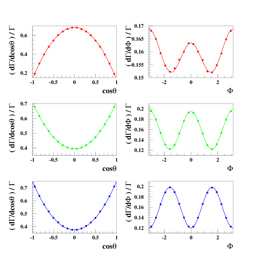
Figure 1: The normalized angular distributions (solid dots) generated according to the matrix element in Eq. (II.1) with S1:$\left(g_{{}_{HZZ}},S^{ZZ}_{H},P^{ZZ}_{H}\right)=(0.1,0,0)$ (upper), S2:$\left(g_{{}_{HZZ}},S^{ZZ}_{H},P^{ZZ}_{H}\right)=(0,0.1,0)$ (middle), and S3:$\left(g_{{}_{HZZ}},S^{ZZ}_{H},P^{ZZ}_{H}\right)=(0,0,0.1)$ (lower). The solid lines are drawn using the analytic expressions for the angular distributions in Eq. (II.3) with $w_{1-9}=1$.

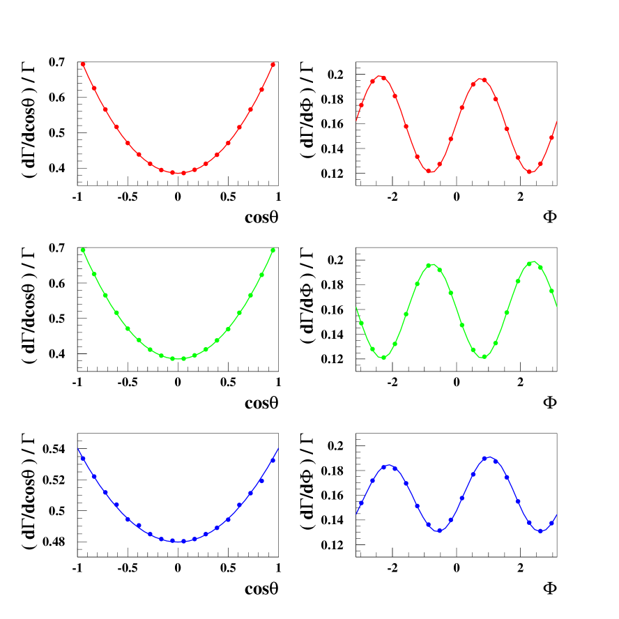
Figure 2: The normalized angular distributions (solid dots) generated according to the matrix element in Eq. (II.1) with S4:$\left(g_{{}_{HZZ}},S^{ZZ}_{H},P^{ZZ}_{H}\right)=(0,0.1,0.1)$ (upper), S5:$\left(g_{{}_{HZZ}},S^{ZZ}_{H},P^{ZZ}_{H}\right)=(0,0.1,-0.1)$ (middle), and S6:$\left(g_{{}_{HZZ}},S^{ZZ}_{H},P^{ZZ}_{H}\right)=(0.032,0.1,0.1)$ (lower). The solid lines are drawn using the analytic expressions for the angular distributions in Eq. (II.3) with $w_{1-9}=1$.

In Table 1, we show the 9 angular coefficients $\overline{C_{1}}-\overline{C_{9}}$ for the 6 scenarios, together with their CP and CP$\widetilde{\rm T}$ parities in the square brackets. With only the real component in the form factors $S_{H}^{ZZ}$ and $P_{H}^{ZZ}$, the coefficients $\overline{C_{2}}$, $\overline{C_{6}}$ and $\overline{C_{7}}$ are identically vanishing in all the scenarios, and $\overline{C_{2}}$, $\overline{C_{5}}$, $\overline{C_{6}}$ and $\overline{C_{9}}$ further vanish in the CP-conserving scenarios of S1, S2, and S3. For S1, $\overline{C_{3}}$ is large due to the enhancement of the longitudinal component $\langle 0\rangle$ of the amplitude for a heavier Higgs boson. Since the longitudinal amplitude $\langle 0\rangle=0$ in the S3 scenario, only $\overline{C_{1}}$ and $\overline{C_{8}}$ take on non-zero values: see Eq. (II.2). In the CP-violating scenarios of S4, S5, and S6, all the coefficients with plus ($+$) CP$\widetilde{\rm T}$ parity are non-vanishing. Note that with $g_{{}_{HZZ}}=0$ in S4 and S5 , the angular coefficient $\overline{C_{3}}=\left|\langle 0\rangle\right|^{2}=4(M_{Z}/M_{H})^{4}$ is suppressed: see Eq. (II.1). All the non-vanishing coefficients are comparable in the scenario S6.

In Table 2, we show the 6 non-vanishing angular observables involved in the one-dimensional angular distributions under the assumption of real $S_{H}^{ZZ}$ and $P_{H}^{ZZ}$, together with the values of $\overline{C_{1}}+\overline{C_{3}}$ for the 6 scenarios. The first and second signs in the square brackets again denote the CP and CP$\widetilde{\rm T}$ parities, respectively. Taking these values we show the angular distributions obtained by the analytic expressions Eq. (II.3): see the solid lines in Figs. 1 and 2. For comparisons we superimpose the angular distributions generated according to Eq. (II.1) as the solid dots.

In the CP-conserving cases shown in Fig. 1, the $\cos\theta_{1,2}$ distribution behaves like $(1-c_{\theta_{1,2}}^{2})$ in scenario S1 because $\overline{R}_{1}\ll 2\overline{R}_{3}$, while the distributions behave like $(1+c_{\theta_{1,2}}^{2})$ with $\overline{R}_{1}\gg 2\overline{R}_{3}$ in scenarios S2 and S3. The $\Phi$ distributions mostly behave according to $\overline{R}_{8}c_{2\Phi}$ with the sub-leading contributions from $\overline{R}_{4}c_{\Phi}$ suppressed by $\eta_{\ell}^{2}$: see Eq. (II.3). The smaller value at $\Phi=0$ compared to those at $\Phi=\pm\pi$ in S1 (upper right) is due to the negative $\overline{R}_{4}c_{\Phi}$ contribution. Note that they are all symmetric about $\Phi=0$ without CP violation.

In the CP-violating scenarios of S4 and S5, the $\cos\theta_{1,2}$ distribution behaves like $(1+c_{\theta_{1,2}}^{2})$ with $\overline{R}_{1}\gg 2\overline{R}_{3}$: see the upper left and middle left frames of Fig. 2. While in S6 with $\overline{R}_{1}$ slightly larger than $2\overline{R}_{3}$, it still behaves as $(1+c_{\theta_{1,2}}^{2})$ but its variation is much smaller compared to the S4 and S5 scenarios due to the cancellation between the $\overline{R}_{1}$ and $\overline{R}_{3}$ terms. The $\Phi$ distributions mostly behave according to $\overline{R}_{8}c_{2\Phi}-\overline{R}_{9}s_{2\Phi}$ with the sub-leading contributions from $\overline{R}_{4}c_{\Phi}-\overline{R}_{5}s_{\Phi}$. We observe that they are no longer symmetric about $\Phi=0$ due to non-trivial phase shift induced by the CP violating terms of $s_{2\Phi}$ and $s_{\Phi}$.

We observe the complete agreement between the angular distributions obtained by the analytic expressions in Eq. (II.3) and those generated according to the helicity amplitude Eq. (II.1), and therefore conclude that our analytic expressions provide an excellent framework to extract the couplings $g_{{}_{HZZ}}$, $S_{H}^{ZZ}$, and $P_{H}^{ZZ}$ and completely measure the properties of a CP-mixed scalar boson $H$ through the angular distributions.

Now we are going to illustrate how well one can measure the properties of the $260$ GeV Higgs by taking the example of scenario S6 with $\left(g_{{}_{HZZ}},S^{ZZ}_{H},P^{ZZ}_{H}\right)=(0.032,0.1,0.1)$, in which all three couplings play almost equal roles. For this purposes we generate a pseudo dataset with the number of events $N_{\rm evt}=10^{3}$ in the range of $\sqrt{k_{1,2}^{2}}=M_{Z}\pm 4$ GeV by noting that the current upper limit on $\sigma(gg\to H)\cdot B(H\to ZZ)\>\raisebox{-2.15277pt}{$\stackrel{{\scriptstyle\textstyle<}}{{\sim}}$}\>0.1$ pb for a 260 GeV Higgs boson at 95 % C.L. h_zz ; atlas17 :

$$\sigma(gg\to H)\cdot B(H\to ZZ)\cdot 4[B(Z\to\ell\ell)]^{2}\cdot\epsilon_{4\ell}\cdot{\cal L}\simeq 10^{3}$$

where we naively take the 4-lepton efficiency $\epsilon_{4\ell}\sim 1$ and assume the HL-LHC with the luminosity of ${\cal L}=3/{\rm ab}$. Further, we assume the angular resolutions of $\Delta\cos\theta=0.1$ and $\Delta\Phi=0.1\pi$.

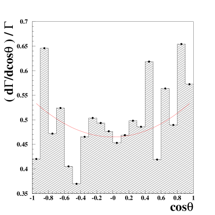
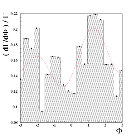
Figure 3: S6: The angular distributions from the pseudo dataset of $N_{\rm evt}=10^{3}$ events generated with $\sqrt{k_{1,2}^{2}}=M_{Z}\pm 4\ {\rm GeV}$, $\Delta\cos\theta=0.1$ and $\Delta\Phi=0.1\pi$. The results of fitting to the angular distributions with Eq. (II.3) are shown in the (red) solid lines.

In Fig. 3, the histograms show the normalized $\cos\theta$ (left) and $\Phi$ (right) distributions from the pseudo dataset of $N_{\rm evt}=10^{3}$ events. Here the $\cos\theta$ distribution is the combination of the $\cos\theta_{1}$ and $\cos\theta_{2}$ distributions. One can obtain the angular observables $\overline{R}_{1,3}$ by fitting to the $\cos\theta$ distribution with the analytic expression for the $1/\Gamma\ {\rm d}\Gamma/{\rm d}c_{\theta_{1,2}}$ in Eq. (II.3). Note we have fixed $\overline{R}_{2}=0$ in the fitting. We have found the strong correlation between the $\overline{R}_{1}$ and $\overline{R}_{3}$ observables with the correlation coefficient $\rho=-0.813$. The angular observables $\overline{R}_{4,5,8,9}$ can be obtained by the Fourier analysis of the $\Phi$ distribution. Explicitly, one may have

$$\overline{R}_{4} = \frac{128}{9\pi^{2}\eta_{\ell}^{2}}\int c_{\Phi}\ \left(\frac{1}{\Gamma}\frac{{\rm d}\Gamma}{{\rm d}\Phi}\right){\rm d}\Phi\,,\ \ \ \overline{R}_{5}=-\ \frac{128}{9\pi^{2}\eta_{\ell}^{2}}\int s_{\Phi}\left(\frac{1}{\Gamma}\frac{{\rm d}\Gamma}{{\rm d}\Phi}\right){\rm d}\Phi\,,$$

$$\overline{R}_{8} = 8\int c_{2\Phi}\ \left(\frac{1}{\Gamma}\frac{{\rm d}\Gamma}{{\rm d}\Phi}\right){\rm d}\Phi\,,\hskip 32.72049pt\overline{R}_{9}=-8\int s_{2\Phi}\ \left(\frac{1}{\Gamma}\frac{{\rm d}\Gamma}{{\rm d}\Phi}\right){\rm d}\Phi\,.$$ (27)

The angular observables $\overline{R}_{4,5,8,9}$ can also be obtained by performing a fit to the $\Phi$ histogram distribution with the analytic expression for the $1/\Gamma\ {\rm d}\Gamma/{\rm d}\Phi$ in Eq. (II.3). We have checked that $\overline{R}_{4,5,8,9}$ from the Fourier analysis and those from the fitting are consistent within errors . In our numerical analysis, we use the fitted angular observables. The results of the fittings are represented by the (red) solid lines in In Fig. 3.

Table 3: The input and output values of the $6$ angular observables $\overline{R}_{1,3,4,5,8,9}$ involved in the one-dimensional angular distributions under the assumption of real $S_{H}^{ZZ}$ and $P_{H}^{ZZ}$. We have taken the scenario S6: $\left(g_{{}_{HZZ}},S^{ZZ}_{H},P^{ZZ}_{H}\right)=(0.032,0.1,0.1)$. The input values are the same as in Table 2. The output values have been obtained by fitting to the $\cos\theta_{1,2}$ and $\Phi$ distributions in Fig. 3. The correlation for $\overline{R}_{1}$ and $\overline{R}_{3}$ is $\rho=-0.813$, while the correlations among others are negligible. For $\overline{C}_{1}+\overline{C}_{3}$, we simply assume 20 % error.

S6	$\ \ \overline{R}_{1}[++]$	$\ \ \overline{R}_{3}[++]$	$\ \ \overline{R}_{4}[++]$	$\ \ \overline{R}_{5}[-+]$	$\ \ \overline{R}_{8}[++]$	$\ \ \overline{R}_{9}[-+]\ \$	$\ \ (\overline{C}_{1}+\overline{C}_{3})[++]\times 10^{2}\ \$
Input	$0.721$	$0.280$	$0.330$	$-0.542$	$-0.331$	$-0.640\ \$	$1.93$
Output (center value)	$0.721$	$0.260$	$-0.339$	$-4.07$	$-0.452$	$-0.387\ \$	$1.93$
Output (parabolic error)	$\pm 0.037$	$\pm 0.034$	$\pm 1.37$	$\pm 1.45$	$\pm 0.17$	$\pm 0.18\ \$	$\pm 0.386$

The details of the fitting results are summarized in Table 3 as the output central values together with the corresponding parabolic errors. We observe that the output central values are within the $1$- or $2$-$\sigma$ ranges of the input values. Note that the CP violation is observed at the $2$-$\sigma$ level with $\overline{R}_{9}=-0.387\pm 0.18$. The observation through another CP-violating observable $\overline{R}_{5}$ is also at the $2$-$\sigma$ level: $\overline{R}_{5}=-4.07\pm 1.45$. First, the error is $8$ times larger than that of $\overline{R}_{9}$ because of the $\eta_{\ell}^{2}$ suppression factor, see Eq. (II.3). Second, this is due to the statistical fluctuation. We have verified that the central values of  the observable $\overline{R}_{5}$ are quite close to the input value $-0.542$ if we generate more pseudo datasets of $10^{3}$ events.

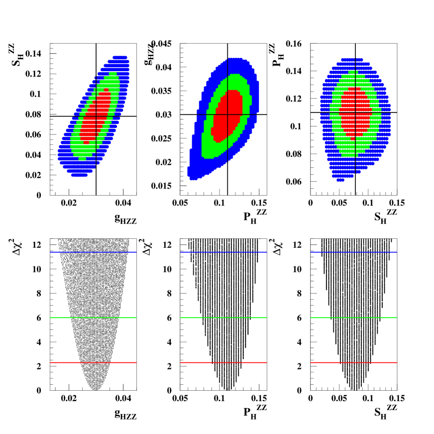
Figure 4: Upper: The confidence-level (CL) regions for scenario S6 $\left(g_{{}_{HZZ}},S^{ZZ}_{H},P^{ZZ}_{H}\right)=(0.032,0.1,0.1)$ with $\Delta\chi^{2}=2.3$ (red), $5.99$ (green), and $11.83$ (blue) above the minimum, which correspond to confidence levels of $68.3\%$, $95\%$, and $99.7\%$, respectively. The vertical and horizontal lines show the best-fit values of $\left(g_{{}_{HZZ}},S^{ZZ}_{H},P^{ZZ}_{H}\right)^{\rm best-fit}=(0.030,0.078,0.11)$. Lower: The scatter plots for $\Delta\chi^{2}$ versus $g_{{}_{HZZ}}$ (left), $\Delta\chi^{2}$ versus $P_{H}^{ZZ}$ (middle), and $\Delta\chi^{2}$ versus $S_{H}^{ZZ}$ (left). The horizontal lines are for the $68.3\%$ (red), $95\%$ (green), and $99.7\%$ (blue) CL regions.

Now we are ready to carry out our ultimate target to extract the couplings $g_{{}_{HZZ}}$, $S_{H}^{ZZ}$, and $P_{H}^{ZZ}$ from the 7 observables $\overline{R}_{1,3,4,5,8,9}$ and $\overline{C}_{1}+\overline{C}_{3}$ by implementing a $\chi^{2}$ analysis. We have taken into account the correlation between $\overline{R}_{1}$ and $\overline{R}_{3}$, by using

$$\chi^{2}(\overline{R}_{1};\overline{R}_{3}) = \Bigg{\{}\frac{\left(\overline{R}_{1}^{\rm TH}-\overline{R}_{1}^{\rm EXP}\right)^{2}}{\left(\sigma_{1}^{\rm EXP}\right)^{2}}+\frac{\left(\overline{R}_{3}^{\rm TH}-\overline{R}_{3}^{\rm EXP}\right)^{2}}{\left(\sigma_{3}^{\rm EXP}\right)^{2}}$$ (28)

$$\hskip 85.35826pt-2\rho\frac{\left(\overline{R}_{1}^{\rm TH}-\overline{R}_{1}^{\rm EXP}\right)}{\sigma_{1}^{\rm EXP}}\frac{\left(\overline{R}_{3}^{\rm TH}-\overline{R}_{3}^{\rm EXP}\right)}{\sigma_{3}^{\rm EXP}}\Bigg{\}}\Bigg{/}(1-\rho^{2})$$

where we calculate $\overline{R}_{1,3}^{\rm TH}$ by varying the three couplings $g_{{}_{HZZ}}$, $S_{H}^{ZZ}$, and $P_{H}^{ZZ}$: see Eqs. (II.1), (II.2), and (19). For $\overline{R}_{1,3}^{\rm EXP}$ and $\sigma_{1,3}^{\rm EXP}$, we have taken the corresponding central output values and errors shown in Table 3. The $\chi^{2}$’s for the remaining uncorrelated observables are similarly calculated and summed.

In the upper frames of Fig. 4, we show the confidence-level regions of the $\chi^{2}$ analysis by varying $g_{{}_{HZZ}}$, $S_{H}^{ZZ}$, and $P_{H}^{ZZ}$. We have found that $\chi^{2}_{\rm min}/d.o.f=7.34/(7-3)=1.83$ and the minimum occurs at

$$g_{{}_{HZZ}}=0.030\pm 0.0035\,;\ \ \ S_{H}^{ZZ}=0.078\pm 0.017\,;\ \ \ P_{H}^{ZZ}=0.11\pm 0.013\,,$$ (29)

which are consistent with the input values $(0.032,0.1,0.1)$ within $\sim 1$-$\sigma$ ranges. Therefore, we conclude that the three couplings of $H$ to a $Z$ boson pair can be determined with about 12-20% errors when $N_{\rm evt}=10^{3}$. We have implemented the similar analysis with $N_{\rm evt}=10^{2}$ and found that the couplings can be determined with about 30% errors.

IV Conclusions

We have performed a comprehensive study of the most general couplings of a spin-0 heavy Higgs boson to a pair of $Z$ bosons up to dimension-6 operators, using the angular distributions in the decay $H\to ZZ\to\ell^{+}\ell^{-}\ell^{+}\ell^{-}$. Based on the helicity amplitude method, we figure out there are 9 types of angular observables $\overline{R}_{i}\,(i=1-9)$ according to their CP and CP$\widetilde{\rm T}$ parities: four of them ($\overline{R}_{2,5,6,9}$) are CP odd and three of them ($\overline{R}_{2,6,7}$) CP$\widetilde{\rm T}$ odd. Furthermore, we find that, among the 9 observables, the 2 CP$\widetilde{\rm T}$-odd observables of $\overline{R}_{6,7}$ are not accessible through one-dimensional angular distributions. We have shown that a certain subset of the 9 angular observables can be extracted from one- and two-dimensional angular distributions of the four final-state charged leptons depending on the assumption on $S^{ZZ}_{H}$ and $P^{ZZ}_{H}$. The parameters $g_{HZZ},S^{ZZ}_{H},P^{ZZ}_{H}$ can then be determined from $\overline{R}_{i}$’s. This is our novel strategy for analyzing the decay $H\to ZZ\to\ell^{+}\ell^{-}\ell^{+}\ell^{-}$ to measure the properties of a heavy Higgs boson $H$.

We have illustrated with $10^{3}$ events for $H\to ZZ\to 4\ell$ that the parameters $g_{HZZ},S^{ZZ}_{H},P^{ZZ}_{H}$ can be determined with only 12-20% uncertainties through the one-dimensional $\cos\theta_{1,2}$ and $\Phi$ distributions under the assumption of real $S^{ZZ}_{H}$ and $P^{ZZ}_{H}$. This is the major numerical result of this work.

We note that following Eq. (II.3) the contributions from the coefficients $C_{4,5}$ to the $\Phi$ distribution are suppressed by the factor $(9\pi^{2}/16)\eta_{\ell}^{2}$ for the decay $ZZ\to 4\ell$, because the vector coupling $v_{\ell}\approx 0.02$ for charged leptons. On the other hand, if we choose the decay $ZZ\to 4b$, the contributions from the coefficients $C_{8,9}$ are suppressed by the numerical factor in front of the term while the contribution from the coefficients $C_{4,5}$ becomes large because $\eta_{b}\simeq 0.936$, and so the $\Phi$ distribution mostly varies as $s_{\Phi}$ and $c_{\Phi}$. In the case of $ZZ\to 2b2l$, all 4 coefficients of $C_{4,5,8,9}$ contribute more or less equally. This interesting possibility will be explored in a future publication FUTURE .

We offer the following further comment in our findings.

1. In principle, the form factors $S^{ZZ}_{H}$ and $P^{ZZ}_{H}$ can be complex when the particles running in the loop are on-shell, e.g, when $M_{H}>2m_{t}$, the absorptive part appears. In such a case, the CP$\widetilde{\rm T}$ angular observables $\overline{R}_{2,6,7}$ are non-vanishing. In this case, the two-dimensional $c_{\theta_{1}}$-$\Phi$ and $c_{\theta_{2}}$-$\Phi$ distributions may provide information on $\overline{R}_{6,7}$ specifically.

Note added: At the last stage of this work, we became aware of a paper atlas17 from ATLAS on search for heavy $ZZ$ resonances in the $\ell^{+}\ell^{-}\ell^{+}\ell^{-}$ and $\ell^{+}\ell^{-}\nu\bar{\nu}$ final states in which, using data at $\sqrt{s}=13$ TeV with the integrated luminosity of 36.1/fb, they report observation of two excesses for $m_{4\ell}$ around 240 and 700 GeV, each with a local significance of $3.6\ \sigma$. Especially, the resonance around 240 GeV corresponds to more than 30 events which may lead to about 3000 events at the HL-LHC with the luminosity of $3/{\rm ab}$, assumed in this work. In this case, we note that the couplings $g_{HZZ},S^{ZZ}_{H},P^{ZZ}_{H}$ can be determined with about 10% uncertainties.

Appendix

Appendix A The four-body phase space

Four-body phase space can be factorized into

$$d\Phi_{4}(Q\to k_{1}k_{2}\to p_{1}\bar{p}_{1}p_{2}\bar{p}_{2}) = d\Phi_{2}(Q\to k_{1}k_{2})\times d\Phi_{2}(k_{1}\to p_{1}\bar{p}_{1})\times d\Phi_{2}(k_{2}\to p_{2}\bar{p}_{2})\times\frac{dk_{1}^{2}}{2\pi}\ \frac{dk_{2}^{2}}{2\pi}$$ (A.1)

$$= \frac{dk_{1}^{2}}{2\pi}\ \frac{dk_{2}^{2}}{2\pi}\ \frac{\lambda^{1/2}(1,k_{1}^{2}/s,k_{2}^{2}/s)}{32\pi^{2}}d\cos\Theta^{*}d\Phi^{*}\$$

$$\times \frac{d\cos\theta_{1}d\phi_{1}}{32\pi^{2}}\ \frac{d\cos\theta_{2}d\phi_{2}}{32\pi^{2}}\$$

where $s=Q^{2}$. For our purpose, we may be able to take

$$d\Phi_{4}(Q\to k_{1}k_{2}\to p_{1}\bar{p}_{1}p_{2}\bar{p}_{2}) = \frac{dk_{1}^{2}}{2\pi}\ \frac{dk_{2}^{2}}{2\pi}\ \frac{\lambda^{1/2}(1,k_{1}^{2}/s,k_{2}^{2}/s)}{8\pi}\frac{d\cos\theta_{1}d\Phi}{32\pi^{2}}\ \frac{d\cos\theta_{2}}{16\pi}\$$ (A.2)

References

- (1) G. Aad et al. [ATLAS Collaboration], “Observation of a new particle in the search for the Standard Model Higgs boson with the ATLAS detector at the LHC,” Phys. Lett. B 716, 1 (2012) [arXiv:1207.7214 [hep-ex]].
- (2) S. Chatrchyan et al. [CMS Collaboration], “Observation of a new boson at a mass of 125 GeV with the CMS experiment at the LHC,” Phys. Lett. B 716, 30 (2012) [arXiv:1207.7235 [hep-ex]].
- (3) See, for example, K. Cheung, J. S. Lee and P. Y. Tseng, “Higgs Precision (Higgcision) Era begins,” JHEP 1305 (2013) 134 doi:10.1007/JHEP05(2013)134 [arXiv:1302.3794 [hep-ph]].
- (4) P. W. Higgs, “Broken Symmetries and the Masses of Gauge Bosons,” Phys. Rev. Lett. 13, 508 (1964); F. Englert and R. Brout, “Broken Symmetry and the Mass of Gauge Vector Mesons,” Phys. Rev. Lett. 13, 321 (1964); G. S. Guralnik, C. R. Hagen and T. W. B. Kibble, “Global Conservation Laws and Massless Particles,” Phys. Rev. Lett. 13, 585 (1964).
- (5) K. Cheung, J. S. Lee and P. Y. Tseng, “Higgs precision analysis updates 2014,” Phys. Rev. D 90 (2014) 095009 doi:10.1103/PhysRevD.90.095009 [arXiv:1407.8236 [hep-ph]].
- (6) For reviews, see, H. P. Nilles, “Supersymmetry, Supergravity and Particle Physics,” Phys. Rept. 110 (1984) 1 doi:10.1016/0370-1573(84)90008-5; H. E. Haber and G. L. Kane, Phys. Rept. 117 (1985) 75 doi:10.1016/0370-1573(85)90051-1; J.F. Gunion, H.E. Haber, G.L. Kane and S. Dawson, The Higgs Hunter’s Guide, (Addison-Wesley, Reading, MA, 1990).
- (7) See, for example, K. Cheung, T. J. Hou, J. S. Lee and E. Senaha, “The Higgs Boson Sector of the Next-to-MSSM with CP Violation,” Phys. Rev. D 82 (2010) 075007 doi:10.1103/PhysRevD.82.075007 [arXiv:1006.1458 [hep-ph]] and references therein.
- (8) See, for example, A. G. Akeroyd and M. Aoki, “Single and pair production of doubly charged Higgs bosons at hadron colliders,” Phys. Rev. D 72 (2005) 035011 doi:10.1103/PhysRevD.72.035011 [hep-ph/0506176] and references therein.
- (9) J. S. Lee, A. Pilaftsis, M. Carena, S. Y. Choi, M. Drees, J. R. Ellis and C. E. M. Wagner, “CPsuperH: A Computational tool for Higgs phenomenology in the minimal supersymmetric standard model with explicit CP violation,” Comput. Phys. Commun. 156 (2004) 283 doi:10.1016/S0010-4655(03)00463-6 [hep-ph/0307377]
- (10) S. Y. Choi, D. J. Miller, M. M. Muhlleitner and P. M. Zerwas, “Identifying the Higgs spin and parity in decays to Z pairs,” Phys. Lett. B 553 (2003) 61 doi:10.1016/S0370-2693(02)03191-X [hep-ph/0210077].
- (11) Y. Gao, A. V. Gritsan, Z. Guo, K. Melnikov, M. Schulze and N. V. Tran, “Spin determination of single-produced resonances at hadron colliders,” Phys. Rev. D 81 (2010) 075022 doi:10.1103/PhysRevD.81.075022 [arXiv:1001.3396 [hep-ph]].
- (12) S. Bolognesi, Y. Gao, A. V. Gritsan, K. Melnikov, M. Schulze, N. V. Tran and A. Whitbeck, “On the spin and parity of a single-produced resonance at the LHC,” Phys. Rev. D 86 (2012) 095031 doi:10.1103/PhysRevD.86.095031 [arXiv:1208.4018 [hep-ph]].
- (13) A. Menon, T. Modak, D. Sahoo, R. Sinha and H. Y. Cheng, “Inferring the nature of the boson at 125-126 GeV,” Phys. Rev. D 89, no. 9, 095021 (2014) doi:10.1103/PhysRevD.89.095021 [arXiv:1301.5404 [hep-ph]].
- (14) T. Modak, D. Sahoo, R. Sinha, H. Y. Cheng and T. C. Yuan, “Disentangling the Spin-Parity of a Resonance via the Gold-Plated Decay Mode,” Chin. Phys. C 40, no. 3, 033002 (2016) doi:10.1088/1674-1137/40/3/033002 [arXiv:1408.5665 [hep-ph]].
- (15) E. Navarro De Martino [CMS Collaboration], “Search for a high mass SM-like Higgs boson in the H to ZZ to llqq decay channel in CMS,” arXiv:1505.03278 [hep-ex]; M. Pelliccioni [CMS Collaboration], “CMS High mass WW and ZZ Higgs search with the complete LHC Run1 statistics,” arXiv:1505.03831 [hep-ex]; The ATLAS collaboration, “Search for high-mass resonances decaying into a Z boson pair in the final state in collisions at TeV with the ATLAS detector,” ATLAS-CONF-2016-012; The ATLAS collaboration [ATLAS Collaboration], “Searches for heavy ZZ and ZW resonances in the llqq and vvqq final states in pp collisions at sqrt(s) = 13 TeV with the ATLAS detector,” ATLAS-CONF-2016-082; CMS Collaboration [CMS Collaboration], “Search for a heavy scalar boson decaying into a pair of Z bosons in the final state,” CMS-PAS-HIG-16-001; CMS Collaboration [CMS Collaboration], “Measurements of properties of the Higgs boson and search for an additional resonance in the four-lepton final state at sqrt(s) = 13 TeV,” CMS-PAS-HIG-16-033.
- (16) K. Hagiwara and D. Zeppenfeld, “Helicity Amplitudes for Heavy Lepton Production in e+ e- Annihilation,” Nucl. Phys. B 274 (1986) 1. doi:10.1016/0550-3213(86)90615-2
- (17) S. von Buddenbrock et al., “The compatibility of LHC Run 1 data with a heavy scalar of mass around 270 GeV,” arXiv:1506.00612 [hep-ph].
- (18) S. von Buddenbrock et al., “Phenomenological signatures of additional scalar bosons at the LHC,” Eur. Phys. J. C 76 (2016) no.10, 580 doi:10.1140/epjc/s10052-016-4435-8 [arXiv:1606.01674 [hep-ph]].
- (19) J. Chang et al., in preparation.
- (20) ATLAS-CONF-2017-058,“ Search for heavy resonances in the and final states using proton-proton collisions at TeV with the ATLAS detector” (5th July 2017).