‘Sinc’-Noise for the KPZ Equation

Abstract

In this paper we study the one-dimensional Kardar-Parisi-Zhang equation (KPZ) with correlated noise by field-theoretic dynamic renormalization group techniques (DRG). We focus on spatially correlated noise where the correlations are characterized by a ‘sinc’-profile in Fourier-space with a certain correlation length $\xi$. The influence of this correlation length on the dynamics of the KPZ equation is analyzed. It is found that its large-scale behavior is controlled by the ‘standard’ KPZ fixed point, i.e. in this limit the KPZ system forced by ‘sinc’-noise with arbitrarily large but finite correlation length $\xi$ behaves as if it were excited with pure white noise. A similar result has been found by Mathey et al. [Phys.Rev.E 95, 032117] in 2017 for a spatial noise correlation of Gaussian type ($\sim e^{-x^{2}/(2\xi^{2})}$), using a different method. These two findings together suggest that the KPZ dynamics is universal with respect to the exact noise structure, provided the noise correlation length $\xi$ is finite.

I Introduction

The ‘standard’ form of the KPZ equation introduced in 1986 by Kardar, Parisi and Zhang, for modeling non-linear growth processes, reads

$$\frac{\partial\,h(x,t)}{\partial t}=\nu\,\nabla^{2}h(x,t)+\frac{\lambda}{2}\,\left(\nabla h(x,t)\right)^{2}+\eta(x,t),$$ (1)

where $h(x,t)$ is a scalar height field (with $x,\,t$ as space and time coordinates, respectively), $\nu$ is a surface tension parameter and $\lambda$ is a non-linear coupling constant. Here $\eta(x,t)$ denotes an uncorrelated Gaussian noise with zero mean (white noise in space and time) Kardar et al. (1986). Therefore the first and second moments of the Gaussian noise are given by

$$\begin{split}\left\langle\eta(x,t)\right\rangle&=0,\\ \left\langle\eta(x,t)\eta(x^{\prime},t^{\prime})\right\rangle&=2\,D\,\delta^{d}(x-x^{\prime})\delta(t-t^{\prime}),\end{split}$$ (2)

where $D$ is a constant amplitude. Besides the noise correlation of (2), various spatially and temporally correlated driving forces have been studied over the years Medina et al. (1989); Forster et al. (1977).

With respect to spatial correlations a widely studied type of driving forces is power-law correlated noise with Fourier-space correlations $\sim q^{-2\rho}$ and $\rho>0$ as a free parameter Medina et al. (1989); Janssen et al. (1999); Kloss et al. (2014). The intriguing observation here is the emergence of a new ‘noise’ fixed point for $\rho>1/4$, additionally to the standard Gaussian and KPZ fixed points.

Recently the KPZ equation with spatially colored and temporally white noise decaying as $\sim e^{-x^{2}/(2\xi^{2})}$ was studied by a non-perturbative DRG analysis in Mathey et al. (2017). It was found that for small values of $\xi$ the KPZ equation behaves in the large-scale limit as if it were stirred by white noise, i.e. with a driving force with vanishing correlation length. Since the non-perturbative RG equations are difficult to solve analytically, the authors of Mathey et al. (2017) relied on numerical techniques.

In the present paper we study the case of spatially correlated noise, where the correlations are characterized by a ‘sinc’-like profile in Fourier-space. As in Mathey et al. (2017), these correlations are characterized by a finite correlation length $\xi$. Unlike Mathey et al. (2017), we solve the problem analytically by using field-theoretic DRG techniques.

For treating ‘sinc’-type noise, we first generalize the field-theoretic DRG formalism for the KPZ equation in such a way that we can handle homogeneous and isotropic noise distributions, whose correlations in momentum space are given by

$$\left\langle\eta(q,\omega)\eta(q^{\prime},\omega^{\prime})\right\rangle=2\,D(|q|^{2})\,\delta^{d}(q+q^{\prime})\,\delta(\omega+\omega^{\prime}).$$ (3)

Note that $D$ does not depend on the frequency, i.e., the noise is spatially colored but temporally white.

For this class of noise correlations, which includes the power-law ($\sim q^{-2\rho}$), Gaussian ($\sim e^{-\xi^{2}q^{2}/2}$) and ‘sinc’-type correlations, the field theoretic DRG formalism will be built in the next section. With the theoretical framework laid out in section II, the explicit ‘sinc’-noise excitation will be analyzed in section III. In section IV the results obtained in section III will be discussed.

II Generalized Field Theoretic Renormalization Group Procedure

A useful tool for building a field theory for stochastic differential equations of type (1) is the effective action $\mathcal{A}[\widetilde{h},h]$, known as the Janssen-De Dominicis response functional Janssen (1976); De Dominicis (1976). Here the action depends on the original height field $h(x,t)$ and the Martin-Siggia-Rose (MSR) auxiliary field $\widetilde{h}(x,t)$.

To derive the effective action, it is useful to transform (3) into real-space:

$$\left\langle\eta(x,t)\eta(x^{\prime},t^{\prime})\right\rangle=2D(x-x^{\prime})\delta(t-t^{\prime}),$$ (4)

where $D(x)=\mathcal{FT}^{-1}\{D(|q|^{2})\}$ Janssen et al. (1999); Kloss et al. (2014).

Using the abbreviations $\underline{y}=(x,t)$ and $\int_{\underline{y}}\cdots=\int d^{d}x\int dt\cdots$, the corresponding Gaussian noise probability distribution can be written as Hochberg et al. (1999)

$$\mathcal{W}[\eta]\propto\exp\left[-\frac{1}{2}\,\int_{\underline{y}}\int_{\underline{y}^{\prime}}\,\eta(\underline{y})\mathcal{M}(\underline{y};\underline{y}^{\prime})\eta(\underline{y}^{\prime})\right],$$ (5)

where $\mathcal{M}(x,t;x^{\prime},t^{\prime})$ is the inverse of the ‘covariance operator’

$$\mathcal{M}^{-1}(x,t;x^{\prime},t^{\prime})=\left\langle\eta(x,t)\eta(x^{\prime},t^{\prime})\right\rangle$$

given in (4), i.e.

$$\begin{split}&\int d^{d}x^{\prime}\int dt^{\prime}\,\mathcal{M}(x,t;x^{\prime},t^{\prime})\mathcal{M}^{-1}(y,\tau;x^{\prime},t^{\prime})\\ &\qquad=\delta^{d}(x-y)\delta(t-\tau).\end{split}$$ (6)

Using (5) and following Refs Canet et al. (2010); Muñoz and Burgett (1989); Hochberg et al. (2000), the expectation value of any observable $O[h]$ can be written as

$$\begin{split}\left\langle O[h]\right\rangle&=\int\mathcal{D}[h]\int\mathcal{D}[i\widetilde{h}]O[h]\exp\left[\int d^{d}x\int dt\,\widetilde{h}(x,t)\left(\partial_{t}h(x,t)-\nu\nabla^{2}h(x,t)-\frac{\lambda}{2}\left(\nabla h(x,t)\right)^{2}\right)\right]\times\\ &\qquad\qquad\times\int\mathcal{D}[\eta]\exp\left[-\frac{1}{2}\,\int d^{d}x\int dt\left(\int d^{d}x^{\prime}\int dt^{\prime}\,\eta(x,t)\mathcal{M}(x,t;x^{\prime},t^{\prime})\eta(x^{\prime},t^{\prime})-\widetilde{h}(x,t)\eta(x,t)\right)\right].\end{split}$$ (7)

Eq. (7) can be rewritten in the form Janssen et al. (1999); Kloss et al. (2014); Canet et al. (2016); Janssen (1976); De Dominicis (1976)

$$\begin{split}\left\langle O[h]\right\rangle&\propto\int\mathcal{D}[h]\,O[h]\mathcal{P}[h]\\ &=\int\mathcal{D}[h]\,O[h]\int\mathcal{D}[i\widetilde{h}]e^{-\mathcal{A}[\widetilde{h},h]},\end{split}$$ (8)

with the Janssen-De Dominicis functional Täuber (2014); Hochberg et al. (1999, 2000); Canet et al. (2011)

$$\begin{split}\mathcal{A}&[\widetilde{h}(x,t),h(x,t)]\\ &=\int_{\underline{y}}\left\{\widetilde{h}(\underline{y})\left(\frac{\partial\,h(\underline{y})}{\partial t}-\nu\nabla^{2}h(\underline{y})-\frac{\lambda}{2}\left(\nabla h(\underline{y})\right)^{2}\right)\right.\\ &\left.\quad-\int d^{d}x^{\prime}\,\widetilde{h}(x,t)D(x-x^{\prime})\widetilde{h}(x^{\prime},t)\right\}.\end{split}$$ (9)

With this functional, one can carry out the usual field-theoretic perturbation expansion in $\lambda$, see e.g. Frey and Täuber (1994); Täuber (2014); Zinn-Justin (2002, 2007).

The KPZ equation is known to be invariant under tilts (Galilei transformation) of the form Frey and Täuber (1994); Janssen et al. (1999)

$$\begin{split}h(x,t)&\to h^{\prime}(x,t)=h(x+\alpha\,\lambda\,t,t)+\alpha\cdot x,\\ \widetilde{h}(x,t)&\to\widetilde{h}^{\prime}(x,t)=\widetilde{h}(x+\alpha\,\lambda\,t,t),\end{split}$$ (10)

where $\alpha$ is the tilting angle. This symmetry is giving rise to two Ward-Takahashi identities. For this reason the KPZ equation has only two independent RG parameters, namely, the noise correlation amplitude $D(x-x^{\prime})$ and the surface tension $\nu$ Frey and Täuber (1994); Janssen et al. (1999).

These parameters are renormalized by

$$\begin{split}D_{R}&=Z_{D}D,\\ \nu_{R}&=Z_{\nu}\nu,\end{split}$$ (11)

where the multiplicative RG factors $Z_{\nu}$ and $Z_{D}$ compensate logarithmic UV divergences occurring in the perturbation integrals. They are related to $\Gamma_{\widetilde{h}h}$ and $\Gamma_{\widetilde{h}\widetilde{h}}$, respectively.

Figure 1: Feynman diagrams for the KPZ equation in a style following Täuber (2014). The left hand diagram shows the one-loop order expansion of the propagator vertex function $\Gamma_{\widetilde{h}h}$, whereas the right hand side depicts the one-loop order expansion of the noise vertex function $\Gamma_{\widetilde{h}\widetilde{h}}$. Here $q$ denotes the outer momentum and $p$ stands for the inner momentum. Note that a symmetrization has already been done, which leads to the noise amplitudes depending on $p\pm q/2$. For reasons of clarity the frequency components carried by each line corresponding to the different momenta are omitted.

The vertex functions $\Gamma_{\widetilde{h}h}$ and $\Gamma_{\widetilde{h}\widetilde{h}}$ will be calculated to one-loop order in Fourier-space for an arbitrary noise with correlations of the form (3).

Denoting the free propagator by $G_{0}(\underline{k})$ ($\underline{k}=(q,\omega)$) and the self energy by $\Sigma(\underline{k})$, the analytic expressions for the diagrams in Fig. 1 are given by the Dyson equation $\Gamma_{\widetilde{h}h}=G_{0}(-\underline{k})^{-1}-\Sigma(\underline{k})$ Zinn-Justin (2007); Amit (1984); Mussardo (2010) and the expansion of the noise vertex $\Gamma_{\widetilde{h}\widetilde{h}}=-2D(q)+\text{{higher orders}}$. Using the usual Feynman rules (see e.g. Täuber (2014)) and integrating out the inner frequencies one obtains

$$\Gamma_{\widetilde{h}h}(\underline{k}) =i\omega+\nu\,q^{2}+\frac{\lambda^{2}}{2\,\nu^{2}}\int_{p}\frac{D(|p-q/2|^{2})(q^{2}/2-q\cdot p)}{(q/2-p)^{2}}\frac{q^{2}/4-p^{2}}{\frac{i\omega}{2\nu}+q^{2}/4+p^{2}}+\mathcal{O}(\lambda^{3}),$$ (12)

$$\Gamma_{\widetilde{h}\widetilde{h}}(\underline{k}) =-2D(|q|^{2})-\frac{\lambda^{2}}{2\,\nu^{3}}\int_{p}\,D(|p+q/2|^{2})D(|p-q/2|^{2})\Re\left[\frac{1}{\frac{i\omega}{2\nu}+q^{2}/4+p^{2}}\right]+\mathcal{O}(\lambda^{3}),$$ (13)

where we used the following abbreviation: $\int_{p}\cdots=1/(2\pi)^{d}\int d^{d}p\cdots$.

Evaluating (12) and (13) it is essential to avoid mixing ultraviolet and infrared divergences of the integrands. One way to keep those divergences separated is to introduce a so-called normalization point (NP). An indiscriminate, however very useful choice is given by Frey and Täuber (1994)

$$\frac{\omega}{2\,\nu}=\mu^{2},\qquad q=0,$$ (14)

where $\mu$ is an arbitrary momentum scale. One advantage of the choice in (14) is that evaluating the integrals in (12) and (13) at $q=0$ yields the possibility of expanding the general noise amplitude $D(|p\pm q/2|^{2})$ about $p$ for $|q|\ll 1$. Hence to order $\mathcal{O}(|q|^{2})$ the momentum-dependent noise amplitude reads

$$D\left(\left|p\pm\frac{q}{2}\right|^{2}\right)=D\left(|p|^{2}\right)\pm(p\cdot q)D^{\prime}\left(|p|^{2}\right)+\mathcal{O}(|q|^{2}).$$ (15)

Using the identities ($d$ is the spatial dimension) Frey and Täuber (1994); Täuber (2014)

$$\int_{p}\,(p\cdot q)^{2}h(|p|,|q|) =\frac{q^{2}}{d}\int_{p}\,p^{2}h(|p|,|q|),$$

$$\int_{p}\,p^{2}(p\cdot q)^{2}h(|p|,|q|) =\frac{q^{2}}{d}\int_{p}\,p^{4}h(|p|,|q|)$$

and inserting (15) into (12) implies at the NP

$$\begin{split}\left.\frac{\partial\,\Gamma_{\widetilde{h}h}}{\partial q^{2}}\right|_{q=0}&=\nu-\frac{\lambda^{2}}{4\,\nu^{2}}\frac{d-2}{d}\int_{p}\frac{D(|p|^{2})}{i\mu^{2}+p^{2}}-\\ &\qquad-\frac{\lambda^{2}}{2\,\nu^{2}}\frac{1}{d}\int_{p}\frac{p^{2}D^{\prime}(|p|^{2})}{i\mu^{2}+p^{2}}.\end{split}$$ (16)

The evaluation of (13) at the NP (14) leads with (15) to

$$\Gamma_{\widetilde{h}\widetilde{h}}=-2D(|q|^{2})-\frac{\lambda^{2}}{2\,\nu^{3}}\int_{p}\left[D(|p|^{2})\right]^{2}\frac{p^{2}}{\mu^{4}+p^{4}}.$$ (17)

From (16) and (17) we obtain the renormalization factors

$$\begin{split}Z_{\nu}&=1-\frac{\lambda^{2}}{4\,\nu^{3}}\frac{d-2}{d}\int_{p}\frac{D(|p|^{2})}{i\mu^{2}+p^{2}}-\\ &\qquad\qquad-\frac{\lambda^{2}}{2\,\nu^{3}}\frac{1}{d}\int_{p}\frac{p^{2}D^{\prime}(|p|^{2})}{i\mu^{2}+p^{2}},\end{split}$$ (18)

$$Z_{D} =1+\frac{1}{D(|q|^{2})\Big{|}_{q=0}}\frac{\lambda^{2}}{4\,\nu^{3}}\int_{p}\left[D(|p|^{2})\right]^{2}\frac{p^{2}}{\mu^{4}+p^{4}}.$$ (19)

These results allow us to compute the Wilson flow functions Janssen et al. (1999); Frey and Täuber (1994); Täuber (2014)

$$\gamma_{D} =\mu\frac{\partial\,}{\partial\mu}\ln Z_{D},$$ (20)

$$\gamma_{\nu} =\mu\frac{\partial\,}{\partial\mu}\ln Z_{\nu},$$ (21)

where the derivative is taken while keeping $D$ and $\nu$ fixed. Likewise, the $\beta$-function is given by

$$\beta_{g}=\mu\frac{\partial\,}{\partial\mu}g_{R},$$ (22)

where

$$g_{R}=gZ_{g}\mu^{d-2}=gZ_{D}Z_{\nu}^{-3}\mu^{d-2}\sim\frac{\lambda^{2}\,D}{4\,\nu^{3}}\mu^{d-2}$$

is a dimensionless effective coupling constant and $D=D(0)$ given in (28).

The dimension of an effective coupling constant in the above form is (see e.g. Frey and Täuber (1994))

$$[g]=\left[\frac{\lambda^{2}\,D}{4\,\nu^{3}}\right]=\mu^{2-d}.$$ (23)

This explains why $g$ has to be multiplied by $\mu^{d-2}$ to render $g_{R}$ dimensionless.

With the flow functions (20)–(22) a partial differential renormalization group equation can be formulated. This RG equation may be solved by using the method of characteristics, where a flow parameter $l$ and an $l$-dependent continuous momentum scale $\widetilde{\mu}(l)=\mu\,l$ is introduced. Those solutions are then used to formulate a KPZ-specific scaling relation for, say, the two point correlation function $C(q,\omega)$. This relation reads Frey and Täuber (1994)

$$C(\mu,D_{R},\nu_{R},g_{R},q,\omega)=q^{-4-2\gamma_{\nu}^{*}+\gamma_{D}^{*}}\hat{C}\left(\frac{\omega}{q^{2+\gamma_{\nu}^{*}}}\right),$$ (24)

where the superscript ‘$*$’ indicates that the Wilson flow functions are evaluated at the stable IR fixed point. A detailed explanation of how the scaling form in (24) is obtained can be found e.g. in Frey and Täuber (1994); Täuber (2014). A comparison of (24) with the general scaling form for the KPZ two-point correlation function in Fourier-space (see e.g. Kardar et al. (1986); Frey and Täuber (1994); Family and Vicsek (1985); Kim and Kosterlitz (1989)), i.e.

$$C(q,\omega)=q^{-d-2\chi-z}\hat{C}\left(\frac{\omega}{q^{z}}\right),$$ (25)

leads to the following expressions for the dynamical exponent $z$ and the roughness exponent $\chi$ Frey and Täuber (1994); Täuber (2014):

$$z =2+\gamma_{\nu}^{*},$$ (26)

$$\chi =1-\frac{d}{2}+\frac{\gamma_{\nu}^{*}-\gamma_{D}^{*}}{2}.$$ (27)

These general considerations will be used in the next part to obtain the critical exponents $z$ and $\chi$ for the explicit ‘sinc’-noise correlation.

III The KPZ Equation with ‘Sinc’-Noise Correlation

We now apply these results to the case of the ‘sinc’-type noise with the correlations

$$\begin{split}\left\langle\eta(q,\omega)\eta(q^{\prime},\omega^{\prime})\right\rangle&=2D(|q|^{2})\delta^{d}(q+q^{\prime})\delta(\omega+\omega^{\prime})\\ &=2D\frac{\sin(\xi|q|)}{\xi|q|}\delta^{d}(q+q^{\prime})\delta(\omega+\omega^{\prime}),\end{split}$$ (28)

where $D$ is a constant noise amplitude, $q\in\mathds{R}^{d}$ and $\xi$ defines the scale of the ‘sinc’-profile.

For simplicity let us consider the case $d=1$. Here the noise distribution transformed back to real-space is a rectangle with size $2\xi\times D/\xi$ centered at $x=0$, which tends to $\delta(x)$ (white noise) in the limit $\xi\to 0$ Kardar et al. (1986).

The first step now is to calculate explicit expressions for the renormalization factors from (18) and (19) for the driving force (28). Thus with

$$D(|p|^{2}) =D\frac{\sin(\xi|p|)}{\xi|p|}$$

and

$$D^{\prime}(|p|^{2}) =\frac{d\,D}{d(|p|^{2})}$$

the renormalization factors read in $d=1$ to one-loop order

$$\begin{split}Z_{\nu}&=1+\frac{D\,\lambda^{2}}{4\,\nu^{3}}\frac{1}{\pi}\left[2\int_{0}^{\infty}dp\,\frac{\sin(\xi p)}{\xi p(i\mu^{2}+p^{2})}-\right.\\ &\left.\qquad-\int_{0}^{\infty}dp\,\frac{\cos(\xi p)}{i\mu^{2}+p^{2}}\right],\end{split}$$ (29)

$$Z_{D} =1+\frac{D\,\lambda^{2}}{4\,\nu^{3}}\frac{1}{\pi}\int_{0}^{\infty}dp\,\frac{\sin^{2}(\xi p)}{\xi^{2}(\mu^{4}+p^{4})}.$$ (30)

The integrals occurring in (29) and (30) can be computed by employing the Residue theorem, which leads to

$$\begin{split}&\qquad Z_{\nu}=1+\frac{D\,\lambda^{2}}{4\,\nu^{3}}\,\frac{e^{-\frac{1}{\sqrt{2}}\xi\,\mu}}{\xi\,\mu^{2}}\times\\ &\times\left[\sin\left(\frac{1}{\sqrt{2}}\xi\,\mu\right)\left(1+\frac{\xi\,\mu}{2\sqrt{2}}\right)-\frac{\xi\,\mu}{2\sqrt{2}}\cos\left(\frac{1}{\sqrt{2}}\xi\,\mu\right)\right],\end{split}$$ (31)

$$\begin{split}&\qquad Z_{D}=1+\frac{D\,\lambda^{2}}{4\,\nu^{3}}\,\frac{e^{-\sqrt{2}\xi\,\mu}}{4\sqrt{2}\xi^{2}\,\mu^{3}}\times\\ &\times\left[e^{\sqrt{2}\xi\,\mu}-\left(\sin(\sqrt{2}\xi\,\mu)+\cos(\sqrt{2}\xi\,\mu)\right)\right].\end{split}$$ (32)

In Appendix A the derivation of these formulas is explained in greater detail.

III.1 Small Correlation Length Expansion

Let us now focus on small correlation lengths $\xi\ll 1$ and expand (31) and (32) in $\xi$ up to order $\mathcal{O}(\xi^{2})$.
Introducing the effective coupling constants Medina et al. (1989)

$$g =\frac{D\,\lambda^{2}}{4\,\nu^{3}},\qquad\quad\>\>g_{R} =\frac{g\,Z_{g}}{2\sqrt{2}\mu};$$ (33)

$$g_{\xi} =\frac{D\,\xi^{2}\,\lambda^{2}}{4\,\nu^{3}},\qquad g_{\xi,R} =\frac{g_{\xi}\,Z_{g}\,\mu}{2\sqrt{2}}.$$ (34)

with $Z_{g}=Z_{D}Z_{\nu}^{-3}$ the one-loop integrals simplify:

$$Z_{\nu} =1+\frac{g}{2\sqrt{2}\mu}-\frac{g_{\xi}\,\mu}{12\sqrt{2}},$$ (35)

$$Z_{D} =1+\frac{g}{2\sqrt{2}\mu}-\frac{D\,\lambda^{2}}{12\,\nu^{3}}\xi+\frac{g_{\xi}\,\mu}{6\sqrt{2}}.$$ (36)

With the renormalized dimensionless effective coupling constants from (33), (34) and using (22) one obtains the flow equations

$$\beta_{g} =g_{R}\left[2g_{R}+\frac{5}{6}g_{\xi,R}-1\right],$$ (37)

$$\beta_{g_{\xi}} =g_{\xi,R}\left[2g_{R}+\frac{5}{6}g_{\xi,R}+1\right].$$ (38)

Solving (37) and (38) for their fixed points $(g^{*},g_{\xi}^{*})$ yields three different possible solutions, namely

$$\begin{split}(g_{R}^{*},g_{\xi,R}^{*})=\begin{cases}(0,0)\quad\text{Gaussian},\\ (0,-\frac{6}{5}),\\ (\frac{1}{2},0)\quad\text{KPZ}.\end{cases}\end{split}$$ (39)

The second one is nonphysical, since $g_{\xi,R}<0$, and thus there are two valid fixed points for the KPZ equation stirred by ‘sinc’-type noise with $\xi\ll 1$.
To determine the stability of the two fixed points we carry out a linear stability analysis via the Jacobian of the two flow functions (37) and (38), i.e.

$$\begin{split}\mathcal{J}&=\begin{pmatrix}\partial_{g_{R}}\beta_{g}&\partial_{g_{\xi,R}}\beta_{g}\\ \partial_{g_{R}}\beta_{g_{\xi}}&\partial_{g_{\xi,R}}\beta_{g_{\xi}}\end{pmatrix}\\ &=\begin{pmatrix}4g_{R}+5/6\,g_{\xi,R}-1&5/6\,g_{R}\\ 2g_{\xi,R}&2g_{R}+5/3\,g_{\xi,R}+1\end{pmatrix}.\end{split}$$ (40)

By evaluating (40) at the respective fixed points it turns out that for the Gaussian fixed point $\mathcal{J}$ is indefinite and for the KPZ fixed point $\mathcal{J}$ is positive definite. Since the condition for asymptotic stability in this framework is positive definiteness of (40), only the KPZ fixed point is stable in the infrared limit and the Gaussian fixed point is unstable.

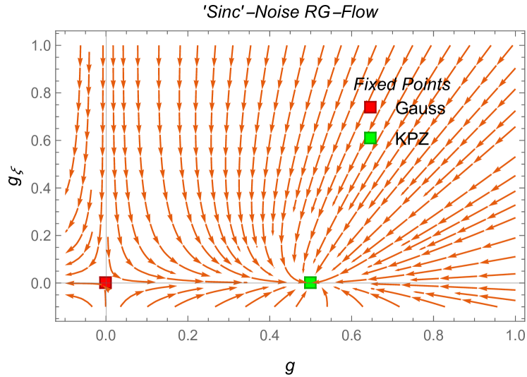
Figure 2: Renormalization group flow of the two effective coupling constants (33) and (34) for small values of the noise correlation length $\xi$ in $d=1$ spatial dimension. As can be seen the only stable infrared fixed point is the KPZ fixed point at $(g,g_{\xi})=(1/2,0)$.

To provide a simple graphical representation of the occurring renormalization group flow Fig. 2 was plotted in Wilson’s picture Wilson (1975). Parametrizing the scale transformation from the field-theoretic to Wilson’s representation by (see e.g. Frey and Täuber (1994))

$$l_{W}=-\ln l$$ (41)

one obtains the following flow equations

$$\frac{d\,\widetilde{g}(l_{W})}{dl_{W}} =-\beta_{g}\stackrel{{\scriptstyle\eqref{Beta_g_Sinc_Expansion}}}{{=}}-\widetilde{g}(l_{W})\left[2\widetilde{g}(l_{W})+\frac{5}{6}\widetilde{g}_{\xi}(l_{W})-1\right],$$ (42)

$$\frac{d\,\widetilde{g}_{\xi}(l_{W})}{dl_{W}} =-\beta_{\xi}\stackrel{{\scriptstyle\eqref{Beta_g_Xi_Sinc_Expansion}}}{{=}}-\widetilde{g}_{\xi}(l_{W})\left[2\widetilde{g}(l_{W})+\frac{5}{6}\widetilde{g}_{\xi}(l_{W})+1\right].$$ (43)

The corresponding RG flow is displayed in Fig. 2.

The critical exponents $z$ and $\chi$ are obtained via (26) and (27). Here the fixed point values of the Wilson flow functions,

$$\gamma_{\nu} =-g_{R}-\frac{g_{\xi,R}}{6}+\mathcal{O}(g_{R}^{2},g_{\xi,R}^{2},g_{R}g_{\xi,R}),$$ (44)

$$\gamma_{D} =-g_{R}+\frac{g_{\xi,R}}{3}+\mathcal{O}(g_{R}^{2},g_{\xi,R}^{2},g_{R}g_{\xi,R}),,$$ (45)

are given by

$$\gamma_{\nu}^{*} =\gamma_{\nu}(g_{R}=1/2,g_{\xi,R}=0)=-\frac{1}{2},$$ (46)

$$\gamma_{D}^{*} =\gamma_{D}(g_{R}=1/2,g_{\xi,R}=0)=-\frac{1}{2}.$$ (47)

Hence the dynamical exponent $z$ and the roughness exponent $\chi$ read

$$z=\frac{3}{2},\qquad\chi=\frac{1}{2}.$$ (48)

They are the same as those in the white-noise case and confirm the KPZ exponent identity $z+\chi=2$ (see e.g. Kardar et al. (1986); Medina et al. (1989); Janssen et al. (1999); Frey and Täuber (1994); Halpin-Healy and Zhang (1995)).

III.2 Arbitrary Correlation Length Calculation

In the following we show that the same result can be derived for arbitrary correlation lengths $\xi$ in $d=1$ dimensions, although the calculations are technically more involved.

Inserting (31), (32) into (21), (20) and expanding to lowest order in the effective coupling constant $g=D\lambda^{2}/(4\nu^{3})$, the Wilson flow functions $\gamma_{i}$ can be written down as

$$\begin{split}\gamma_{\nu}&=\mu\frac{\partial\,\ln Z_{\nu}}{\partial\mu}=-\frac{g_{R}}{Z_{\nu}}\frac{e^{-\frac{1}{\sqrt{2}}\xi\,\mu}}{\xi\,\mu}\left[\left(3\xi\,\mu+4\sqrt{2}\right)\sin\frac{\xi\,\mu}{\sqrt{2}}-\xi\,\mu\left(\sqrt{2}\xi\,\mu+3\right)\cos\frac{\xi\,\mu}{\sqrt{2}}\right]\\ &=-g_{R}\frac{e^{-\frac{1}{\sqrt{2}}\xi\,\mu}}{\xi\,\mu}\left[\left(3\xi\,\mu+4\sqrt{2}\right)\sin\frac{\xi\,\mu}{\sqrt{2}}-\xi\,\mu\left(\sqrt{2}\xi\,\mu+3\right)\cos\frac{\xi\,\mu}{\sqrt{2}}\right]+\mathcal{O}(g_{R}^{2}),\end{split}$$ (49)

$$\begin{split}\gamma_{D}&=\mu\frac{\partial\,\ln Z_{D}}{\partial\mu}=\frac{g_{R}}{Z_{D}}\frac{e^{-\sqrt{2}\xi\,\mu}}{2\xi^{2}\,\mu^{2}}\left[\left(2\sqrt{2}\xi\,\mu+3\right)\sin\sqrt{2}\xi\,\mu-3\left(e^{\sqrt{2}\xi\,\mu}-\cos\sqrt{2}\xi\,\mu\right)\right]\\ &=g_{R}\frac{e^{-\sqrt{2}\xi\,\mu}}{2\xi^{2}\,\mu^{2}}\left[\left(2\sqrt{2}\xi\,\mu+3\right)\sin\sqrt{2}\xi\,\mu-3\left(e^{\sqrt{2}\xi\,\mu}-\cos\sqrt{2}\xi\,\mu\right)\right]+\mathcal{O}(g_{R}^{2}),\end{split}$$ (50)

where we introduced the dimensionless form of the renormalized couplings

$$g_{R}=\frac{g\,Z_{g}}{2\sqrt{2}\mu},\qquad Z_{g}=Z_{D}Z_{\nu}^{-3}.$$ (51)

The corresponding $\beta$-function (22) reads

$$\beta_{g}=g_{R}\left[g_{R}\left(\widetilde{\gamma}_{D}-3\widetilde{\gamma}_{\nu}\right)-1\right],$$ (52)

where $\widetilde{\gamma_{i}}=\gamma_{i}/g_{R}$ and $\gamma_{\nu}$, $\gamma_{D}$ are taken from (49), (50), respectively.

Again the flow of the effective coupling constant is modeled via the flow parameter $l$ used for the solution of the RG equations by the method of characteristics. This leads to a continuous momentum scale $\widetilde{\mu}(l)$, effective coupling constant $\widetilde{g}(l)$ and thus to an $l$-dependent flow equation (see e.g. Frey and Täuber (1994); Janssen et al. (1999))

$$\beta_{g}(l)=l\frac{d\,\widetilde{g}(l)}{dl}.$$ (53)

Hence a fixed point is characterized by $\beta_{g}(l)=0$. Applying this fixed point condition to (52) and solving for $g_{R}$ leads to two separate infrared fixed point solutions $g_{R,i}^{*}$:

$$g_{R,1}^{*} =0,$$ (54)

$$g_{R,2}^{*} =\lim_{l\to 0}\frac{1}{\widetilde{\gamma}_{D}(l)-3\widetilde{\gamma}_{\nu}(l)}.$$ (55)

Here (54) represents the trivial Gaussian fixed point while the second solution in the limit $l\to 0$ Täuber (2014) yields the nontrivial KPZ fixed point,

$$g_{R,2}^{*}=\lim_{l\to 0}\frac{1}{\widetilde{\gamma}_{D}(l)-3\widetilde{\gamma}_{\nu}(l)}=\frac{1}{2}.$$ (56)

Again the fixed points are stable, if $d\beta_{g}/dg_{R}>0$. Since (49), (50), (52) imply that

$$\beta_{g}^{\prime}=\frac{d\,\beta_{g}(l)}{d\widetilde{g}(l)}=2\widetilde{g}(l)\left(\widetilde{\gamma}_{D}(l)-3\widetilde{\gamma}_{\nu}(l)\right)-1\stackrel{{\scriptstyle l\to 0}}{{=}}4g_{R}-1,$$ (57)

we find that:

$$g_{R}^{*} =0 :\qquad\beta_{g}^{\prime} =-1<0\quad \Longrightarrow\text{unstable},$$

$$g_{R}^{*} =\frac{1}{2} :\qquad\beta_{g}^{\prime} =1>0\quad \Longrightarrow\text{stable}.$$

Hence there is one stable infrared fixed point, $g_{R}^{*}=1/2$, at which the critical exponents of the KPZ universality class can be calculated.

We obtain the critical exponents in $d=1$ dimensions again as

$$z =2+\gamma_{\nu}^{*}=2-\frac{1}{2}=\frac{3}{2},$$ (58)

$$\chi =\frac{1}{2}+\frac{-\frac{1}{2}+\frac{1}{2}}{2}=\frac{1}{2}.$$ (59)

IV Discussion

In the present work we have studied the field-theoretic DRG of the KPZ equation for correlated noise of ‘sinc’-type which is characterized by a finite correlation     length $\xi$.

The fixed points of the KPZ-DRG flow have been calculated in two different manners, namely first for small correlation lengths $\xi$ and via two effective coupling constants, $g$ and $g_{\xi}$ (see subsection III.1 and (33), (34)) and then, using only one effective coupling constant $g$ (see subsection III.2), for arbitrary values of $\xi$. Both methods yield the same results, i.e., an unstable Gaussian fixed point (see (39), (54)) and the stable KPZ fixed point (see (39), (56)).

It might be argued, that the second method is somewhat redundant since the ‘small’-$\xi$ expansion can also be interpreted to be valid for arbitrary values of $\xi$ in the infrared limit as in this regime $\mu\to 0$ and hence $\xi\,\mu\eqqcolon\epsilon\ll 1$. The expansion would then be done for the parameter $\epsilon$. Nevertheless, the method used in subsection III.2 is a reassuring confirmation of the results obtained in subsection III.1.

Building on these fixed points, the critical exponents characterizing the KPZ universality class, i.e. the dynamical exponent $z=3/2$ and the roughness exponent $\chi=1/2$, were calculated (see (48) and (58), (59)). The values obtained for $z$ and $\chi$ coincide with the ‘standard’ KPZ exponents in one spatial dimension, where the system is excited by purely white noise (see e.g.Kardar et al. (1986); Frey and Täuber (1994)).

Hence, for every finite noise correlation length $\xi$ the system behaves to one-loop order as if it was stirred by the ‘standard’ uncorrelated Gaussian noise from (2).

This result corresponds nicely with the numerical findings of Mathey et al. (2017), where a different spatial noise correlation was analyzed. The authors there found that for small values of the noise correlation length the KPZ equation acted like it was driven by pure white noise.

Combining the findings of Mathey et al. (2017) with the present ones, found for different noise functions and by different methods, we arrive at the conjecture that the large-scale KPZ dynamics is independent of the details of the noise structure, provided that the correlation length $\xi$ is finite.

Appendix A Explicit Evaluation of the Renormalization Factors

To obtain (31), (32) from the expressions in (29), (30), respectively, we use the Residue theorem. To this end the integrals are first rewritten in a more easily accessible form.

A.1 Evaluation of Eq. (29)

The first integral needed for the calculation of $Z_{\nu}$ reads

$$\int_{0}^{\infty}dp\,\frac{\sin(\xi\,p)}{\xi\,p(i\mu^{2}+p^{2})}.$$ (60)

This may be rewritten as

$$\int_{0}^{\infty}dp\,\frac{\sin(\xi\,p)}{\xi\,p(i\mu^{2}+p^{2})}=-\frac{i}{2}\int_{-\infty}^{\infty}dp\,\frac{e^{i\xi\,p}}{\xi\,p(i\mu^{2}+p^{2})}$$ (61)

The integrand on the r.h.s. in (61) has three simple poles which are given by $z_{1/2}=\pm\mu\,e^{i3\pi/4}$ and $z_{3}=0$. Those and the chosen integration contour are shown in Fig. 3.

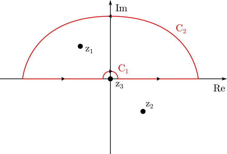
Figure 3: Integration contour $C$ for the evaluation of (60). $C_{1}$ and $C_{2}$ are circles about $z=0$ with radius $\epsilon$ and $R$, respectively.

Hence the residue theorem yields

$$\quad\int_{C}dz\,\frac{e^{i\xi z}}{\xi z(i\mu^{2}+z^{2})}$$

$$=\int_{-R}^{-\epsilon}dz\,\frac{e^{i\xi z}}{\xi z\left(i\mu^{2}+z^{2}\right)}+\int_{C_{1}}dz\,\frac{e^{i\xi z}}{\xi z\left(i\mu^{2}+z^{2}\right)}+$$

$$\qquad+\int_{\epsilon}^{R}dz\,\frac{e^{i\xi z}}{\xi z\left(i\mu^{2}+z^{2}\right)}+\int_{C_{2}}dz\,\frac{e^{i\xi z}}{\xi z\left(i\mu^{2}+z^{2}\right)}$$

$$=2\,\pi\,i\lim_{z\to\mu\,e^{i3\pi/4}}\frac{\left(z-\mu\,e^{i3\pi/4}\right)e^{i\xi z}}{\xi z\left(z-\mu\,e^{i3\pi/4}\right)\left(z+\mu\,e^{i3\pi/4}\right)}$$

$$=-\frac{\pi\,e^{-\frac{1}{\sqrt{2}}\xi\mu}}{\xi\mu^{2}}\left[\cos\left(\frac{1}{\sqrt{2}}\xi\mu\right)-i\sin\left(\frac{1}{\sqrt{2}}\xi\mu\right)\right].$$

To obtain the integral on the real axis from minus to plus infinity, the contributions of the integrals over the two circular paths have to be computed. Therefore the parametrization

$$z=\epsilon\,e^{i\varphi}\quad\Leftrightarrow\quad dz=i\,\epsilon\,e^{i\varphi}d\varphi$$

is used, which yields for the integral over $C_{1}$ with $\epsilon\to 0$:

$$\lim_{\epsilon\to 0}\int_{C_{1}}dz\,\frac{e^{i\xi z}}{\xi z\left(i\mu^{2}+z^{2}\right)}$$

$$\quad=-\lim_{\epsilon\to 0}\int_{0}^{\pi}d\varphi\,\frac{i\,e^{i\xi\epsilon e^{i\varphi}}}{\xi\left(i\mu^{2}+\epsilon^{2}\,e^{2i\varphi}\right)}$$

$$\quad=-\int_{0}^{\pi}d\varphi\,\lim_{\epsilon\to 0}\frac{i\,e^{i\xi\epsilon e^{i\varphi}}}{\xi\left(i\mu^{2}+\epsilon^{2}\,e^{2i\varphi}\right)}=-\frac{\pi}{\xi\,\mu^{2}}$$

For the integration over the contour $C_{2}$ a similar parametrization is used

$$z=R\,e^{i\varphi}\quad\Leftrightarrow\quad dz=i\,R\,e^{i\varphi}d\varphi.$$ (62)

The contribution from this integral vanishes for $R\to\infty$:

$$\lim_{R\to\infty}\left|\int_{C_{2}}dz\,\frac{e^{i\xi z}}{\xi z\left(i\mu^{2}+z^{2}\right)}\right|$$

$$\quad=\lim_{R\to\infty}\left|\int_{0}^{\pi}d\varphi\,\frac{i\,R\,e^{i\xi Re^{i\varphi}}e^{i\varphi}}{\xi Re^{i\varphi}\left(i\mu^{2}+R^{2}e^{2i\varphi}\right)}\right|$$

$$\quad\leq\lim_{R\to\infty}\int_{0}^{\pi}d\varphi\,\frac{\left|e^{i\xi Re^{i\varphi}}\right|}{\left|\xi\left(i\mu^{2}+R^{2}e^{2i\varphi}\right)\right|}$$

$$\quad=\lim_{R\to\infty}\int_{0}^{\pi}d\varphi\,\frac{e^{-\xi R\sin\varphi}}{\xi R^{2}\left|i\frac{\mu^{2}}{R^{2}}+e^{2i\varphi}\right|}=0,$$

since $\sin\varphi>0$ for $0<\varphi<\pi$. Thus in the limits $R\to\infty$ and $\epsilon\to 0$ the residue theorem results in

$$\int_{-\infty}^{\infty}dz\,\frac{e^{i\xi z}}{\xi z\left(i\mu^{2}+z^{2}\right)}=\frac{\pi\,e^{-\frac{1}{\sqrt{2}}\xi\mu}}{\xi\,\mu^{2}}\left[e^{\frac{1}{\sqrt{2}}\xi\mu}-\right.$$

$$\left.\qquad\qquad\qquad-\left(\cos\left(\frac{1}{\sqrt{2}}\xi\mu\right)-i\sin\left(\frac{1}{\sqrt{2}}\xi\mu\right)\right)\right].$$

The integral from (60) is therefore given by

$$\begin{split}&\int_{0}^{\infty}dp\,\frac{\sin(\xi p)}{\xi p\left(i\mu^{2}+p^{2}\right)}=\pi\frac{e^{-\frac{1}{\sqrt{2}}\xi\mu}}{2\,\xi\,\mu^{2}}\times\\ &\quad\times\left[\sin\left(\frac{1}{\sqrt{2}}\xi\mu\right)+i\left(\cos\left(\frac{1}{\sqrt{2}}\xi\mu\right)-e^{\frac{1}{\sqrt{2}}\xi\mu}\right)\right].\end{split}$$ (63)

The second integral needed for the evaluation of (29) is given by

$$\int_{0}^{\infty}dp\,\frac{\cos(\xi\,p)}{i\mu^{2}+p^{2}}.$$ (64)

As for the calculation of (60), the integral will be rewritten according to

$$\int_{0}^{\infty}dp\,\frac{\cos(\xi\,p)}{i\mu^{2}+p^{2}}=\frac{1}{2}\int_{-\infty}^{\infty}dp\,\frac{e^{i\xi\,p}}{i\mu^{2}+p^{2}}.$$ (65)

The integrand on the r.h.s. of (65) has two simple poles at $z_{1/2}=\pm\,\mu\,e^{i3\pi/4}$. For the integration contour shown in Fig. 4, the residue theorem leads to

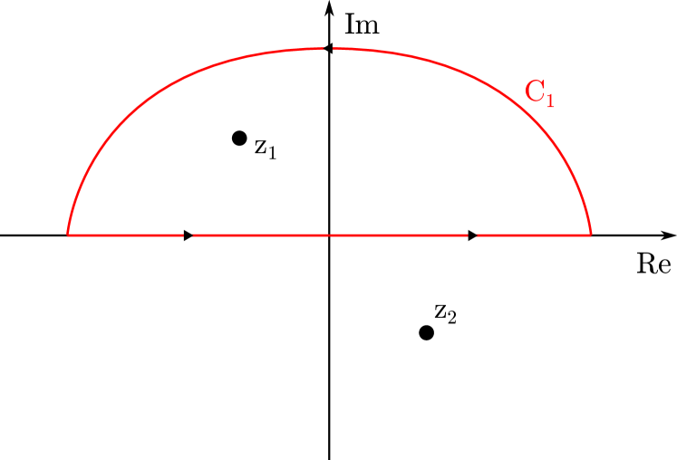
Figure 4: This diagram shows the contour $C$ of integration for (65). $C_{1}$ denotes a circle about $z=0$ with radius $R$.

$$\int_{C}dz\,\frac{e^{i\xi z}}{i\mu^{2}+z^{2}}=\int_{-R}^{R}dz\,\frac{e^{i\xi z}}{i\mu^{2}+z^{2}}+\int_{C_{1}}dz\,\frac{e^{i\xi z}}{i\mu^{2}+z^{2}}$$

$$\quad=2\,\pi\,i\lim_{z\to\mu e^{i3\pi/4}}\frac{\left(z-\mu\,e^{i3\pi/4}\right)e^{i\xi z}}{\left(z-\mu\,e^{i3\pi/4}\right)\left(z+\mu\,e^{i3\pi/4}\right)}$$

$$\quad=\frac{\pi\,e^{-\frac{1}{\sqrt{2}}\xi\mu}}{\sqrt{2}\,\mu}\left(\cos\left(\frac{1}{\sqrt{2}}\xi\mu\right)-\sin\left(\frac{1}{\sqrt{2}}\xi\mu\right)-\right.$$

$$\left.\qquad-i\left[\cos\left(\frac{1}{\sqrt{2}}\xi\mu\right)+\sin\left(\frac{1}{\sqrt{2}}\xi\mu\right)\right]\right)$$

Choosing again the parametrization (62) it is readily shown that its contribution vanishes for $R\to\infty$:

$$\qquad\lim_{R\to\infty}\left|\int_{C_{1}}dz\,\frac{e^{i\xi z}}{i\mu^{2}+z^{2}}\right|$$

$$=\lim_{R\to\infty}\left|\int_{0}^{\pi}d\varphi\,\frac{i\,R\,e^{i\xi Re^{i\varphi}}e^{i\varphi}}{i\mu^{2}+R^{2}\,e^{2i\varphi}}\right|$$

$$\leq\lim_{R\to\infty}\int_{0}^{\pi}d\varphi\,\frac{\left|i\,R\,e^{i\xi Re^{i\varphi}}e^{i\varphi}\right|}{\left|i\mu^{2}+R^{2}\,e^{2i\varphi}\right|}$$

$$=\lim_{R\to\infty}\int_{0}^{\pi}d\varphi\,\frac{e^{-\xi R\sin\varphi}}{R\left|\frac{i\mu^{2}}{R^{2}}+e^{2i\varphi}\right|}=0$$

Hence the sought integral reads

$$\begin{split}&\int_{0}^{\infty}dp\,\frac{\cos(\xi p)}{i\mu^{2}+p^{2}}\\ &\quad=\pi\frac{e^{-\frac{1}{\sqrt{2}}\xi\mu}}{2\,\sqrt{2}\,\mu}\left(\cos\left(\frac{1}{\sqrt{2}}\xi\mu\right)-\sin\left(\frac{1}{\sqrt{2}}\xi\mu\right)-\right.\\ &\left.\qquad-i\left[\cos\left(\frac{1}{\sqrt{2}}\xi\mu\right)+\sin\left(\frac{1}{\sqrt{2}}\xi\mu\right)\right]\right).\end{split}$$ (66)

Taking the real parts Janssen et al. (1999) of (63) and (66) and inserting the results into (29) leads to the expression in (31).

A.2 Evaluation of Eq. (30)

The integral (30) reads

$$\begin{split}&\frac{1}{\pi}\int_{0}^{\infty}dp\,\frac{\sin^{2}(\xi p)}{\mu^{4}+p^{4}}\\ &\quad=\frac{1}{2\pi}\left[\int_{0}^{\infty}dz\,\frac{1}{\mu^{4}+z^{4}}-\int_{0}^{\infty}dz\,\frac{\cos(2\xi z)}{\mu^{4}+z^{4}}\right].\end{split}$$ (67)

The integrands of both integrals in (67) have simple poles at $z_{k}=\mu\,e^{i(\pi/4+\pi k/2)}$, with $k=0,1,2,3$, and the contour of integration is shown in Fig. 5.

Figure 5: Representation of the zeros and the contour $C$ of integration for the two integrals on the right hand side of (67). $C_{1}$ is again a circle with radius $R$ about $z=0$.

The first of the two integrals on the right hand side of (67) is readily solved with the aid of the residue theorem (again it can be shown that $\int_{C_{1}}dz/(\mu^{4}+z^{4})=0$ for $R\to\infty$):

$$\begin{split}&\qquad\int_{0}^{\infty}dz\,\frac{1}{\mu^{4}+z^{4}}=\frac{1}{2}\int_{-\infty}^{\infty}dz\,\frac{1}{\mu^{4}+p^{4}}\\ &=\frac{1}{2}2\,\pi\,i\left[\lim_{z\to z_{0}}\frac{z-z_{0}}{(z-z_{0})(z-z_{1})(z-z_{2})(z-z_{3})}+\right.\\ &\left.\quad+\lim_{z\to z_{1}}\frac{z-z_{1}}{(z-z_{0})(z-z_{1})(z-z_{2})(z-z_{3})}\right]\\ &=\frac{\pi}{2\sqrt{2}\mu^{3}}.\end{split}$$ (68)

For the second integral it is again used that

$$2\int_{0}^{\infty}dz\,\frac{\cos(2\xi z)}{\mu^{4}+z^{4}}=\int_{-\infty}^{\infty}\frac{e^{2i\xi z}}{\mu^{4}+z^{4}}\qquad(z\in\mathds{R}).$$

With the integration contour shown in Fig. 5, we arrive at

$$\qquad\int_{-R}^{R}dz\,\frac{e^{2i\xi z}}{\mu^{4}+z^{4}}+\int_{C_{1}}dz\,\frac{e^{2i\xi z}}{\mu^{4}+z^{4}}$$

$$=2\,\pi\,i\left[\lim_{z\to z_{0}}\frac{\left(z-z_{0}\right)e^{2i\xi z}}{\left(z-z_{0}\right)\left(z-z_{1}\right)\left(z-z_{2}\right)\left(z-z_{3}\right)}+\right.$$

$$\left.\quad+\lim_{z\to z_{1}}\frac{\left(z-z_{1}\right)e^{2i\xi z}}{\left(z-z_{0}\right)\left(z-z_{1}\right)\left(z-z_{2}\right)\left(z-z_{3}\right)}\right]$$

$$=\frac{\pi\,e^{-\sqrt{2}\xi\mu}}{\sqrt{2}\mu^{3}}\left[\cos(\sqrt{2}\xi\mu)+\sin(\sqrt{2}\xi\mu)\right].$$

As $\int_{C_{1}}dze^{2i\xi z}/(\mu^{4}+z^{4})$ tends to zero for $R\to\infty$,

$$\lim_{R\to\infty}\left|\int_{0}^{\pi}d\varphi\,\frac{iRe^{i\varphi}e^{2i\xi Re^{i\varphi}}}{\mu^{4}+R^{4}e^{4i\varphi}}\right|$$

$$\quad\leq\lim_{R\to\infty}\int_{0}^{\pi}d\varphi\,\frac{\left|iRe^{i\varphi}e^{2i\xi Re^{i\varphi}}\right|}{\left|\mu^{4}+R^{4}e^{4i\varphi}\right|}$$

$$\quad=\lim_{R\to\infty}\int_{0}^{\pi}d\varphi\frac{e^{-2\xi R\sin\varphi}}{R^{3}\left|\frac{\mu^{4}}{R^{4}}+e^{4i\varphi}\right|}=0,$$

it is found that

$$\int_{0}^{\infty}dz\,\frac{\cos(2\xi z)}{\mu^{4}+z^{4}}=\frac{\pi\,e^{-\sqrt{2}\xi\mu}}{2\sqrt{2}\mu^{3}}\left[\cos(\sqrt{2}\xi\mu)+\sin(\sqrt{2}\xi\mu)\right].$$ (69)

The results from (68) and (69), inserted into (30), yield the expression in (32).