Moving object tracking employing rigid body motion on matrix Lie groups

Abstract

In this paper we propose a novel method for estimating rigid body motion by modeling the object state directly in the space of the rigid body motion group $\text{SE}(2)$. It has been recently observed that a noisy manoeuvring object in $\text{SE}(2)$ exhibits banana-shaped probability density contours in its pose. For this reason, we propose and investigate two state space models for moving object tracking: (i) a direct product $\text{SE}(2)\times{\mathbb{R}}^{3}$ and (ii) a direct product of the two rigid body motion groups $\text{SE}(2)\times\text{SE}(2)$. The first term within these two state space constructions describes the current pose of the rigid body, while the second one employs its second order dynamics, i.e., the velocities. By this, we gain the flexibility of tracking omnidirectional motion in the vein of a constant velocity model, but also accounting for the dynamics in the rotation component. Since the $\text{SE}(2)$ group is a matrix Lie group, we solve this problem by using the extended Kalman filter on matrix Lie groups and provide a detailed derivation of the proposed filters. We analyze the performance of the filters on a large number of synthetic trajectories and compare them with (i) the extended Kalman filter based constant velocity and turn rate model and (ii) the linear Kalman filter based constant velocity model. The results show that the proposed filters outperform the other two filters on a wide spectrum of types of motion.

I Introduction

A wide area of robotics research has extensively focused on the practical approaches of using different types of manifolds. Besides performance, filters operating on manifolds can provide other advantages as they avoid singularities when representing state spaces with either redundant degrees of freedom or constraint issues [1, 2]. Among the manifolds, the homogeneous transformation matrices, also referred to as the rigid body motion group $\text{SE}(n)$, hold a special repute. They have been used in a variety of applications, and have risen to popularity firstly through manipulator robotics [3, 4] and later through vision applications [5, 6]. Even though the state description using the rigid body motion group, for both the $2$D and $3$D case, has been a well known representation, techniques for associating the uncertainty came into focus later [7]. So far, the rigid body motion group with associated uncertainty has been used in several robotics applications such as SLAM [8], motion control [9], shape estimation [10], pose estimation [11] and pose registration [12].

Among them, pose estimation represents one of the central problems in robotics. Recently in [11] the authors discussed the advantages of employing uncertainties on $\text{SE}(2)$ (therein called the exponential coordinates) with respect to Euclidean spaces and have provided the means for working in the exponential coordinates rather than representing the robot’s position with Gaussians in Cartesian coordinates. This stems from the fact that the uncertain robot motion, and consequently its pose, usually exhibit banana-shaped probability density contours rather than the elliptical ones [13], as illustrated in Fig. 1.

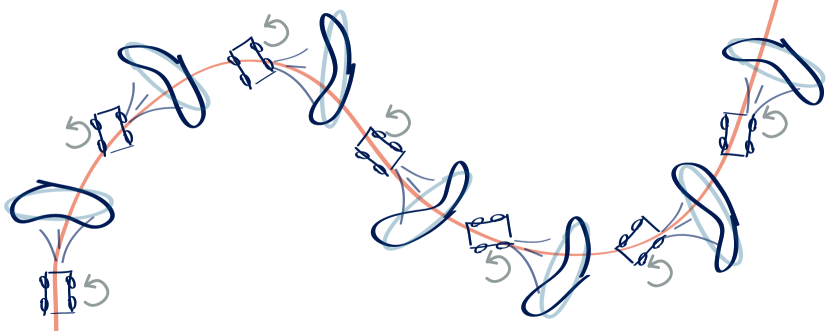
Figure 1: An illustration of an omnidirectional mobile robot manoeuvring in both translational and rotational components. The banana shaped uncertainty contours, representing the positional uncertainty in the next step, are formed by modeling the uncertainty on the $\text{SE}(2)$ group (blue), while the elliptical shaped contours appear modeling the uncertainty in ${\mathbb{R}}^{2}$ (gray).

The classical Kalman filter is designed to operate in the Cartesian space and as such does not provide a framework for filtering directly on the $\text{SE}(2)$ group. Recently, some works have addressed the uncertainty on the $\text{SE}(2)$ group proposing new distributions [14, 15]. However, these interesting approaches do not yet provide a closed-form Bayesian recursion framework (involving both the prediction and update) that can include higher order motion and non-linear models.

An extended Kalman filter on matrix Lie groups (LG-EKF) has been recently proposed in [16]. It provides an estimation framework for filtering directly on matrix Lie groups, of which the $\text{SE}(2)$ group is a member. In accordance with the needs of moving object state estimation problems, higher order motion often needs to be exploited, as in the vein of the constant velocity (CV) or acceleration motion models [17], but in the space such as the rigid body motion group $\text{SE}(2)$. In the present paper we propose a method for moving object tracking employing its second order motion directly on the $\text{SE}(2)$ group based on the discrete LG-EKF. For this purpose, we model the state space either as a direct product of (i) a rigid body motion group and a Euclidean vector or (ii) two rigid body motion groups, i.e.,

$$\text{(i) }\text{SE}(2)\times{\mathbb{R}}^{3}\text{ \ or \ }\text{(ii) }\text{SE}(2)\times\text{SE}(2)=\text{SE}(2)^{2}.$$ (1)

In both cases the first term tracks the pose of the object, while the second one handles the velocities. In the end, we conduct experimental validation of the proposed filters on synthetic data and compare their performance with the CV and constant turn rate and velocity (CTRV) motion models [18] used within the classical extended Kalman filter (EKF) framework.

The rest of the paper is organized as follows. Section II gives an insight into the motivation behind the present paper. Section III provides the preliminaries including the basic definitions and operators for working with matrix Lie groups, with emphasis on the special euclidean group $\text{SE}(2)$. The method for exploiting higher order motion is presented in Section IV and the proposed estimation strategies are investigated on a synthetic dataset and compared with two Kalman filter based methods. Finally, concluding remarks are drawn in Section V.

II Motivation

The choice of the state space and the approach to the motion modelling present a significant focus of this paper. The physical interpretation behind associating the uncertainty with the $\text{SE}(2)$ group has been analyzed in [11]. Therein, the authors particularly study the shape of the uncertainty by considering differential drive mobile robot motion. The authors conclude that the $\text{SE}(2)$ approach provides significant flexibility in describing the position uncertainty, enabling one to analytically work with banana-shaped uncertainty contours. In this work, given the previous moving object tracking discussion, we aim to track omnidirectional motion in order to achieve high flexibility in motion modeling. This is motivated by considering tracking in unknown dynamic environments comprising of multiple unknown moving objects. For example, a mobile robot building a map of an unknown environment consisting of humans and other robots with various kinematics, or a busy intersection with mixed traffic involving cars, trams, motorcycles, bicycles and pedestrians.

By searching for the flexibility to control the velocities in both $x$ and $y$ direction, as well as the rotational velocity, one comes to formulation of the state space as $\text{SE}(2)\times{\mathbb{R}}^{3}$. In this case, the $\text{SE}(2)$ term tracks the pose of a rigid body object supporting the forming of banana-shaped uncertainty contours, while the ${\mathbb{R}}^{3}$ term describes velocities along the three axis in a classical manner forming elliptical-only contours. Examples of omnidirectional mechanical robot platforms implementations which can be described by this state space construction are the Palm Pilot Robot, Uranus, and Killough [19], which are based on the Swedish $45^{\circ}$/$90^{\circ}$ wheels.

However, if we consider a robot construction that has additional flexibility of controling the steering angle of one or more wheels, it turns out that by sampling such kinematic models the uncertainty in the space of velocities also has banana-shaped contours. Given that, we further propose to model the state space as $\text{SE}(2)^{2}$ group where now the second term exploits the second order motion (velocities), and supports the flexibility of forming the banana-shaped uncertainty contours in the velocity space. Examples of mechanical omnidirectional robot platforms capable of such motion are the Nomad XR4000 and Hyperion [19]. Detailed physical and kinematic interpretations of these models are, however, out of the scope of this paper and are a subject for future work.

III Preliminaries

III-A Lie groups and Lie algebra

In this section, we provide notations and properties for matrix Lie groups and the associated Lie algebras which will be used for the filter including the $\text{SE}(2)$ group in the state space. For a more formal introduction of the used concepts, the interested reader is directed to [20], where the author provides a rigorous treatment of representing and propagating uncertainty on matrix Lie groups.

The $\text{SE}(2)$, specifically, is a matrix Lie group. A Lie group is a group which has the structure of a smooth manifold, i.e., it is sufficiently often differentiable [2], such that group composition and inversion are smooth operations. Furthermore, for a matrix Lie group G these operations are simply matrix multiplication and inversion, with the identity matrix $\text{I}^{n\times n}$ being the identity element [20]. An interesting property of Lie groups, basically curved objects, is that they can be almost completely captured by a flat object, such as the tangential space; and this leads us to an another important concept—the Lie algebra $\mathfrak{g}$ associated to a Lie group G.

Lie algebra $\mathfrak{g}$ is an open neighborhood of $\boldsymbol{0}^{n\times n}$ in the tangent space of G at the identity $\text{I}^{n\times n}$. The matrix exponential $\exp_{\text{G}}$ and matrix logarithm $\log_{\text{G}}$ establish a local diffeomorphism between these two worlds, i.e., Lie groups and Lie algebras

$$\exp_{\text{G}}:\mathfrak{g}\rightarrow\text{G}\text{ \ and \ }\log_{\text{G}}:\text{G}\rightarrow\mathfrak{g}.$$ (2)

The Lie algebra $\mathfrak{g}$ associated to a $p$-dimensional matrix Lie group $\text{G}\subset{\mathbb{R}}^{n\times n}$ is a $p$-dimensional vector space defined by a basis consisting of $p$ real matrices $E_{i}$, $i=1,..,p$ [9]. A linear isomorphism between $\mathfrak{g}$ and ${\mathbb{R}}^{p}$ is given by

$$[\cdot]^{\vee}_{\text{G}}:\mathfrak{g}\rightarrow{\mathbb{R}}^{p}\text{ \ and \ }[\cdot]^{\wedge}_{\text{G}}:{\mathbb{R}}^{p}\rightarrow\mathfrak{g}.$$ (3)

Lie groups are not necessarily commutative and require the use two operators to capture this property and thus, enable the adjoint representation of (i) G on ${\mathbb{R}}^{p}$ denoted as $\operatorname{Ad}_{\text{G}}$ and (ii) ${\mathbb{R}}^{p}$ on ${\mathbb{R}}^{p}$ denoted as $\operatorname{ad}_{\text{G}}$ [20]. All the discussed operators in the present section are presented later in the paper for the proposed state space constructions.

III-B Concentrated Gaussian Distribution

Another important concept in the LG-EKF framework is that of the concentrated Gaussian distribution (CGD). In order to define the CGD on matrix Lie groups, the considered group needs to be a connected unimodular matrix Lie group [21], which is the case for the majority of martix Lie groups used in robotics.

Let the probability density function (pdf) of $X$, a state on a $p$-dimensional matrix Lie group G, be defined as [22]

$$p(X)=\beta\exp\left({-\dfrac{1}{2}[\log_{\text{G}}(X)]^{\vee^{T}}_{\text{G}}}P^{-1}[\log_{\text{G}}(X)]^{\vee}_{\text{G}}\right)\,,$$ (4)

where $\beta$ is a normalizing constant chosen such that (4) integrates to unity. In general $\beta\neq(2\pi)^{-p/2}|P|^{-1/2}$ with $|\cdot|$ being the matrix determinant and $P$ a positive definite matrix.

Furthermore, let $\epsilon$ be defined as $\epsilon\triangleq[\log_{\text{G}}(X)]^{\vee}_{\text{G}}$. If we now assume that the entire mass of probability is contained inside G, then $\epsilon$ can be described by $\epsilon\sim\mathcal{N}_{{\mathbb{R}}^{p}}(\boldsymbol{0}^{p\times 1},P)$. This represents the CGD on G around the identity [16]. Furthermore, it is a unique parametrization space where the bijection between $\exp_{\text{G}}$ and $\log_{\text{G}}$ exists. Now, the pdf of $X$ can be ‘translated’ over the G by using the left action of the matrix Lie group

$$X=\mu\exp_{\text{G}}\left([\epsilon]^{\wedge}_{\text{G}}\right)\ \text{, with}\ \ X\sim\mathcal{G}(\mu,P)\,,$$ (5)

where $\mathcal{G}$ denotes the concentrated Gaussian distribution [22, 16] with the mean $\mu$ and the covariance matrix $P$. In other words, the mean $\mu$ of the state $X$ resides on the $p$-dimensional matrix Lie group G, while the associated uncertainty is defined in the space of the Lie algebra $\mathfrak{g}$, i.e., by the linear isomorphism the Euclidean vector space ${\mathbb{R}}^{p}$. By this, we have introduced the distribution forming the base for the LG-EKF.

III-C The $\text{SE}(2)$ group

The motion group $\text{SE}(2)$ describes the rigid body motion in $2$D and is formed as a semi-direct product of the plane ${\mathbb{R}}^{2}$ and the special orthogonal group $\text{SO}(2)$ corresponding to translational and rotational parts, respectively. It is defined as

$$\text{SE}(2)=\left\{\begin{pmatrix}R&\boldsymbol{t}\\ \boldsymbol{0}^{1\times 1}&1\end{pmatrix}\in{\mathbb{R}}^{3\times 3}\,|\,\{R,\boldsymbol{t}\}\in\text{SO}(2)\times{\mathbb{R}}^{2}\right\}\,.$$ (6)

Now, we continue with providing the basic ingredients for handling $\text{SE}(2)$, giving the relations for operators from III-A, needed for manipulation between the triplet (Lie group G, Lie algebra $\mathfrak{g}$, Euclidean space ${\mathbb{R}}^{p}$).

For the Euclidean spaced vector $\boldsymbol{x}=\begin{bmatrix}x\ y\ \theta\end{bmatrix}^{T}$, the most often associated element of the Lie algebra $\mathfrak{se}(2)$ is given as

$$[\boldsymbol{x}]^{\wedge}_{\text{SE}(2)}=\begin{bmatrix}0&-\theta&x\\ \theta&0&y\\ 0&0&0\end{bmatrix}\in\mathfrak{se}(2)\,.$$ (7)

Correspondingly, its inverse $[\cdot]^{\vee}_{\text{SE}(2)}$ is trivial.

The exponential map for the $\text{SE}(2)$ group is given as

$$\exp_{\text{SE}(2)}([\boldsymbol{x}]^{\wedge}_{\text{G}})=\begin{bmatrix}\cos\theta&-\sin\theta&t_{x}\\ \sin\theta&\cos\theta&t_{y}\\ 0&0&1\end{bmatrix}\in\text{SE}(2)$$ (8)

$$\qquad t_{x}=\frac{1}{\theta}\left[x\sin\theta+y(-1+\cos\theta)\right]$$ (9)

$$\qquad t_{y}=\frac{1}{\theta}\left[x(1-\cos\theta)+y\sin\theta)\right]\,.$$ (10)

For $T=\{R,\boldsymbol{t}\}\in\text{SE}(2)$, the logarithmic map is

$$\log_{\text{SE}(2)}(T)=\begin{bmatrix}\boldsymbol{v}\\ \theta\end{bmatrix}^{\wedge}_{\text{SE}(2)}\in\mathfrak{se}(2)$$ (11)

$$\qquad\theta=\log_{\text{SO}(2)}(R)=\operatorname{atan2}2(R_{21},R_{11})$$ (12)

$$\qquad\boldsymbol{v}=\dfrac{\theta}{2(1-\cos\theta)}\begin{bmatrix}\sin\theta&1-\cos\theta\\ \cos\theta-1&\sin\theta\end{bmatrix}\boldsymbol{t}\,.$$ (13)

The Adjoint operator $\operatorname{Ad}_{\text{G}}$ used for representing $T\in\text{SE}(2)$ on ${\mathbb{R}}^{3}$ is given as

$$\operatorname{Ad}_{\text{SE}(2)}(T)=\begin{bmatrix}R&J\boldsymbol{t}\\ \boldsymbol{0}^{1\times 2}&1\end{bmatrix}\ \text{with}\ J=\begin{bmatrix}0&1\\ -1&0\end{bmatrix}\,.$$ (14)

The adjoint operator $\operatorname{ad}_{\text{G}}$ for representing $\boldsymbol{x}\in{\mathbb{R}}^{3}$ on ${\mathbb{R}}^{3}$ is given by

$$\operatorname{ad}_{\text{SE}(2)}(\boldsymbol{x})=\begin{bmatrix}-\theta J&J\boldsymbol{v}\\ \boldsymbol{0}^{1\times 2}&1\end{bmatrix}\,,$$ (15)

where $\boldsymbol{v}=[x\ y]^{T}\in{\mathbb{R}}^{2}$.

IV Rigid body motion tracking

IV-A EKF on matrix Lie groups

For the general filtering approach on matrix Lie groups, the system is assumed to be modeled as satisfying the following equation [23]

$$\begin{split}X_{k+1}=f(X_{k},n_{k})=X_{k}\,\exp_{\text{G}}\left([\hat{\Omega}_{k}+n_{k}]^{\wedge}_{\text{G}}\right)\,,\end{split}$$ (16)

where $X_{k}\in\text{G}$ is the state of the system at time $k$, G is a $p$-dimensional Lie group, $n_{k}\sim\mathcal{N}_{{\mathbb{R}}^{p}}(\boldsymbol{0}^{p\times 1},Q_{k})$ is white Gaussian noise and $\hat{\Omega}_{k}=\Omega(X_{k}):\text{G}\rightarrow{\mathbb{R}}^{p}$ is a non-linear $\mathcal{C}^{2}$ function.

The prediction step of the LG-EKF, based on the motion model (16), is governed by the following formulae

$$\mu_{k+1|k} =\mu_{k}\exp_{\text{G}}\left([\hat{\Omega}_{k}]^{\wedge}_{\text{G}}\right)$$ (17)

$$P_{k+1|k} =\mathcal{F}_{k}P_{k}\mathcal{F}_{k}^{T}+\Phi_{\text{G}}(\hat{\Omega}_{k})Q_{k}\Phi_{\text{G}}(\hat{\Omega}_{k})^{T}\,,$$ (18)

where $\mu_{k+1|k}\in\text{G}$ and $P_{k+1|k}\in{\mathbb{R}}^{p\times p}$ are predicted mean value and the covariance matrix, respectively, hence the state remains $\mathcal{G}$–distributed $X_{k+1|k}\sim\mathcal{G}(\mu_{k+1|k},P_{k+1|k})$. The operator $\mathcal{F}_{k}$, a matrix Lie group equivalent to the Jacobian of $f(X_{k},n_{k})$, and $\Phi_{\text{G}}$ are given as follows

$$\mathcal{F}_{k} =\text{Ad}_{\text{G}}\left(\exp_{\text{G}}\left([-\hat{\Omega}_{k}]^{\wedge}_{\text{G}}\right)\right)+\Phi_{\text{G}}(\hat{\Omega}_{k})\mathscr{C}_{k}$$ (19)

$$\Phi_{\text{G}}(\boldsymbol{v}) =\sum_{m=0}^{\infty}\dfrac{(-1)^{m}}{(m+1)!}\operatorname{ad}_{\text{G}}(\boldsymbol{v})^{m}\,,\ \boldsymbol{v}\in{\mathbb{R}}^{p}$$ (20)

$$\mathscr{C}_{k} =\dfrac{\partial}{\partial\epsilon}\Omega\left(\mu_{k}\exp_{\text{G}}\left([\epsilon]^{\wedge}_{\text{G}}\right)\right)_{|\epsilon=0}\,.$$ (21)

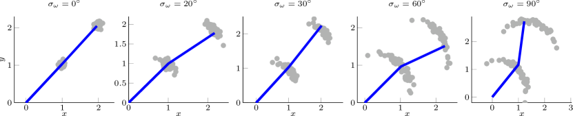
Figure 2: Each of the subfigures represents an example of two compounding transformations for different levels of rotational uncertainty (given in blue). The grey circles represent $50$ sampled uncertain transformations by employing both translational and rotational uncertainties. This particular situation appears when a robot moves from the current position to the next position associated with the next discrete moment in time, with standard deviation of the rotation $\sigma_{\omega}$.

The discrete measurement model on the matrix Lie group is modelled as

$$Z_{k+1}=h(X_{k+1})\,\exp_{\text{G}^{\prime}}\left([m_{k+1}]^{\wedge}_{\text{G}^{\prime}}\right)\,,$$ (22)

where $Z_{k+1}\in\text{G}^{\prime}$, $h:\text{G}\rightarrow\text{G}^{\prime}$ is a $\mathcal{C}^{1}$ function and $m_{k+1}\sim\mathcal{N}_{{\mathbb{R}}^{q}}(\boldsymbol{0}^{q\times 1},R_{k+1})$ is white Gaussian noise.

The update step of the filter, based on the measurement model (22), strongly resembles the standard EKF update procedure, relying on the Kalman gain $K_{k+1}$ and innovation vector $\nu_{k+1}$ calculated as follows

$$K_{k+1} =P_{k+1|k}{\mathcal{H}}_{k+1}^{T}\left({\mathcal{H}}_{k+1}P_{k+1|k}{\mathcal{H}}_{k+1}^{T}+R_{k+1}\right)^{-1}$$

$$\nu_{k+1} =K_{k+1}\left(\left[\log_{\text{G}^{\prime}}\left(h(\mu_{k+1|k})^{-1}Z_{k+1}\right)\right]^{\vee}_{\text{G}^{\prime}}\right)\,.$$ (23)

The matrix ${\mathcal{H}}_{k}$ can be seen as the measurement matrix of the system, i.e., a matrix Lie group equivalent to the Jacobian of $h(X_{k})$, and is given as

$$\begin{split}{\mathcal{H}}_{k+1}=\dfrac{\partial}{\partial\epsilon}&\left[\log_{\text{G}^{\prime}}\left(h(\mu_{k+1|k})^{-1}\right.\right.\\ &\left.\left.h\left(\mu_{k+1|k}\exp_{\text{G}}\left([\epsilon]^{\wedge}_{\text{G}}\right)\right)\right)\right]^{\vee}_{\text{G}\ |\epsilon=0}\,.\end{split}$$ (24)

Finally, having defined all the constituent elements, the update step is calculated via

$$\mu_{k+1} =\mu_{k+1|k}\exp_{\text{G}}\left([\nu_{k+1}]^{\wedge}_{\text{G}}\right)$$ (25)

$$P_{k+1} =\Phi_{\text{G}}(\nu_{k+1})\left(\text{I}^{p\times p}-K_{k+1}{\mathcal{H}}_{k+1}\right)P_{k+1|k}\Phi_{\text{G}}(\nu_{k+1})^{T}\,.$$ (26)

As in the case of the prediction step, the state $X_{k+1}\sim\mathcal{G}(\mu_{k+1},P_{k+1})$ remains $\mathcal{G}$–distributed after the correction as well. For a more formal derivation of the LG-EKF, the interested reader is referred to [16].

Since the employment of the $\text{SE}(2)\times{\mathbb{R}}^{3}$ follows the similar, but slightly simpler derivation, in the sequel we derive the LG-EKF filter for estimation on the state space modelled as $\text{SE}(2)^{2}$. This approach is in our case applied, but not limited, to the problem of moving object tracking.

IV-B LG-EKF on $\text{SE}(2)^{2}$

As mentioned previously, we model the state $X$ to evolve on the matrix Lie group $\text{G}=\text{SE}(2)^{2}$ which is symbolically represented by

$$X=\begin{bmatrix}\begin{bmatrix}R_{\theta}&\boldsymbol{t}\\ \boldsymbol{0}^{1\times 2}&1\end{bmatrix}&\\ &\begin{bmatrix}R_{\omega}&\boldsymbol{t}_{v}\\ \boldsymbol{0}^{1\times 2}&1\end{bmatrix}\end{bmatrix}=\begin{pmatrix}T_{s}\\[2.84526pt] T_{d}\end{pmatrix}_{\text{G}}\,,$$ (27)

where $T_{s}$ is the stationary component and $T_{d}$ brings the second order dynamics. Note that the matrix Lie group composition and inversion are simple matrix multiplication and inversion, hence the previous symbolic representation can be used for all the calculations dealing with operations on G.

The Lie algebra associated to the Lie group G is denoted as $\mathfrak{g}=\mathfrak{se}(2)^{2}$, thereby for $\boldsymbol{x}=\begin{bmatrix}\boldsymbol{x}_{p}\ \boldsymbol{x}_{d}\end{bmatrix}^{T}\in{\mathbb{R}}^{6}$, where $\boldsymbol{x}_{p}=\begin{bmatrix}x\ y\ \theta\end{bmatrix}^{T}$ and $\boldsymbol{x}_{d}=\begin{bmatrix}v_{x}\ v_{y}\ \omega\end{bmatrix}^{T}$, the following holds

$$[\boldsymbol{x}]^{\wedge}_{\text{G}}=\begin{bmatrix}\left[\boldsymbol{x}_{p}\right]^{\wedge}_{\text{SE}(2)}&\\ &\left[\boldsymbol{x}_{d}\right]^{\wedge}_{\text{SE}(2)}\end{bmatrix}=\begin{pmatrix}\left[\boldsymbol{x}_{p}\right]^{\wedge}_{\text{SE}(2)}\\[5.69054pt] \left[\boldsymbol{x}_{d}\right]^{\wedge}_{\text{SE}(2)}\end{pmatrix}_{\mathfrak{g}}.$$ (28)

The exponential map for such defined G is

$$\exp_{\text{G}}([\boldsymbol{x}]^{\wedge}_{\text{G}})=\begin{pmatrix}\exp_{\text{SE}(2)}\left(\left[\boldsymbol{x}_{p}\right]^{\wedge}_{\text{SE}(2)}\right)\\[5.69054pt] \exp_{\text{SE}(2)}\left(\left[\boldsymbol{x}_{d}\right]^{\wedge}_{\text{SE}(2)}\right)\end{pmatrix}_{\text{G}}\,.$$ (29)

Now, we have all the necessary ingredients for deriving the terms to be used within the LG-EKF. Several examples of the uncertain transformations following the $\text{SE}(2)^{2}$ motion model are shown in Fig. 2 (the $\text{SE}(2)\times{\mathbb{R}}^{3}$ model would exhibit similar behaviour).

IV-B1 Prediction

We propose to model the motion (16) of the system by

$$\Omega(X_{k}) =\begin{bmatrix}Tv_{x_{k}}\ Tv_{y_{k}}\ T\omega_{k}\ 0\ 0\ 0\ \end{bmatrix}^{T}\in{\mathbb{R}}^{6}\,,$$ (30)

$$n_{k} =\begin{bmatrix}\frac{T^{2}}{2}n_{x_{k}}\ \frac{T^{2}}{2}n_{y_{k}}\ \frac{T^{2}}{2}n_{\omega_{k}}\ Tn_{x_{k}}\ Tn_{y_{k}}\ Tn_{\omega_{k}}\ \end{bmatrix}^{T}\in{\mathbb{R}}^{6}\,.$$

With such a defined motion model, the system is corrupted with white noise over three separated components, i.e., $n_{x}$ the noise in the local $x$ direction, $n_{y}$ the noise in the local $y$ direction and $n_{w}$ as the noise in the rotational component. Given that, the intensity of the noise components acts as acceleration over the associated axes in the system. If the system state at the discrete time step $k$ is described with $X_{k}\sim\mathcal{G}(\mu_{k},P_{k})$, the mean value and the covariance can be propagated using (17) and (18).

The covariance propagation is more challenging, since it requires the calculation of (21). For the Lie algebraic error $\epsilon\triangleq\begin{bmatrix}\epsilon_{x}\ \epsilon_{y}\ \epsilon_{\theta}\ \epsilon_{v_{x}}\ \epsilon_{v_{y}}\ \epsilon_{\omega}\end{bmatrix}$, we need to set the following

$$\begin{split}&\Omega\left(\mu_{k}\exp_{\text{G}}\left([\epsilon]^{\wedge}_{\text{G}}\right)\right)\\ &\hskip 2.84544pt=\begin{bmatrix}\Delta Tv_{x_{k}}+\Delta T\cos\omega_{k}\,v_{1}-\Delta T\sin\omega_{k}\,v_{2}\\ \Delta Tv_{y_{k}}+\Delta T\sin\omega_{k}\,v_{1}+\Delta T\cos\omega_{k}\,v_{2}\\ \Delta T\omega_{k}+\Delta T\epsilon_{\omega}\\ \boldsymbol{0}^{3\times 1}\end{bmatrix}\,.\end{split}$$ (31)

where

$$\begin{split}v_{1}&=\left[\epsilon_{v_{x}}\sin\epsilon_{\omega}+\epsilon_{v_{y}}(\cos\epsilon_{\omega}-1)\right]\epsilon_{\omega}^{-1}\\ v_{2}&=\left[\epsilon_{v_{x}}(1-\cos\epsilon_{\omega})+\epsilon_{v_{y}}\sin\epsilon_{\omega}\right]\epsilon_{\omega}^{-1}.\end{split}$$ (32)

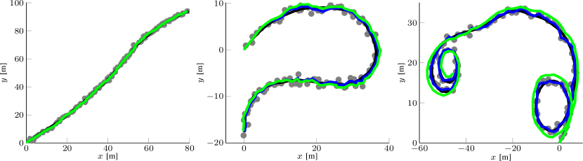
Figure 3: Examples of three different simulated trajectories, generated with the $\text{SE}(2)^{2}$ motion model, with different intensities of process noise over rotational components, i.e., standard deviation in rotational component was $\sigma_{\omega}=[0.01\ 0.1\ 1]^{\circ}$. The blue line corresponds to $\text{SE}(2)^{2}$ filter, while the green line represents the CV model ($\text{SE}(2)\times{\mathbb{R}}^{3}$ and CTRV are omitted for clarity).

Let $\Omega_{1,k}$, $\Omega_{2,k}$ and $\Omega_{3,k}$ denote the first three rows of the vector (31), respectively (whereas the last three rows are trivial $\Omega_{4,k}=\Omega_{5,k}=\Omega_{6,k}=0$).

$$\begin{split}\dfrac{\partial\Omega_{1,k}}{\partial\epsilon_{v_{x}}}|_{\epsilon=0}&=\Delta T\cos\omega_{k}\frac{\sin\epsilon_{\omega}}{\epsilon_{\omega}}-\Delta T\sin\omega_{k}\frac{\cos\epsilon_{\omega}-1}{\epsilon_{\omega}}|_{\epsilon=0}=\Delta T\cos\omega_{k}\\ \dfrac{\partial\Omega_{1,k}}{\partial\epsilon_{v_{y}}}|_{\epsilon=0}&=\Delta T\cos\omega_{k}\frac{\cos\epsilon_{\omega}-1}{\epsilon_{\omega}}-\Delta T\sin\omega_{k}\frac{\sin\epsilon_{\omega}}{\epsilon_{\omega}}|_{\epsilon=0}=-\Delta T\sin\omega_{k}\\ \dfrac{\partial\Omega_{1,k}}{\partial\epsilon_{\omega}}|_{\epsilon=0}&=\Delta T\cos\omega\dfrac{(\epsilon_{v_{x}}\cos\epsilon_{\omega}-\epsilon_{v_{y}}\sin\epsilon_{\omega})\epsilon_{\omega}-[\epsilon_{v_{x}}\sin\epsilon_{\omega}+\epsilon_{v_{y}}(\cos\epsilon_{\omega}-1)]}{\epsilon_{\omega}^{2}}\\ &-\Delta T\sin\omega\dfrac{(\epsilon_{v_{x}}\sin\epsilon_{\omega}+\epsilon_{v_{y}}\cos\epsilon_{\omega})\epsilon_{\omega}-[\epsilon_{v_{x}}(\cos\epsilon_{\omega}-1)+\epsilon_{v_{y}}\sin\epsilon_{\omega}]}{\epsilon_{\omega}^{2}}|_{\epsilon=0}=0\\ \dfrac{\partial\Omega_{2,k}}{\partial\epsilon_{v_{x}}}|_{\epsilon=0}&=\Delta T\sin\omega_{k}\,,\quad\dfrac{\partial\Omega_{2,k}}{\partial\epsilon_{v_{y}}}|_{\epsilon=0}=\Delta T\cos\omega_{k}\,,\quad\dfrac{\partial\Omega_{2,k}}{\partial\epsilon_{\omega}}|_{\epsilon=0}=0\\ \dfrac{\partial\Omega_{3,k}}{\partial\epsilon_{v_{x}}}|_{\epsilon=0}&=0\,,\quad\dfrac{\partial\Omega_{3,k}}{\partial\epsilon_{v_{y}}}|_{\epsilon=0}=0\,,\quad\dfrac{\partial\Omega_{3,k}}{\partial\epsilon_{\omega}}|_{\epsilon=0}=\Delta T\end{split}$$ (33)

Even though the multivariate limits $\dfrac{\partial\Omega_{1,k}}{\partial\epsilon_{\omega}}|_{\epsilon=0}$ and $\dfrac{\partial\Omega_{2,k}}{\partial\epsilon_{\omega}}|_{\epsilon=0}$ appear involved, their derivation follow from patient algebraic manipulations. The resulting terms are shown in (33). The matrix $\mathscr{C}_{k}$ is finally then given as

$$\mathscr{C}_{k}=\begin{bmatrix}\boldsymbol{0}^{3\times 3}&\begin{matrix}\Delta T\cos\omega_{k}&-\Delta T\sin\omega_{k}&0\\ \Delta T\sin\omega_{k}&\Delta T\cos\omega_{k}&0\\ 0&0&\Delta T\end{matrix}\\ \boldsymbol{0}^{3\times 3}&\boldsymbol{0}^{3\times 3}\end{bmatrix}\,.$$ (34)

The adjoint operators $\operatorname{Ad}_{\text{G}}$ and $\operatorname{ad}_{\text{G}}$ are formed block diagonally as

$$\begin{split}\operatorname{Ad}_{\text{G}}(X)&=\text{diag}\left(\operatorname{Ad}_{\text{SE}(2)}(T_{s}),\,\operatorname{Ad}_{\text{SE}(2)}(T_{d})\right)\,,\\[2.84526pt] \operatorname{ad}_{\text{G}}(\boldsymbol{x})&=\text{diag}\left(\operatorname{ad}_{\text{SE}(2)}(\boldsymbol{x}_{s}),\,\operatorname{ad}_{\text{SE}(2)}(\boldsymbol{x}_{d})\right)\,.\end{split}$$ (35)

The last needed ingredient is the process noise covariance matrix $Q_{k}$. Assuming the constant acceleration over the sampling period $\Delta T$, we model the process noise as a discrete white noise acceleration over the three components: $n_{x_{k}}$, $n_{y_{k}}$ and $n_{\omega_{k}}$. At this point, we can use the equation (18) for predicting the covariance of the system.

IV-B2 Update

The predicted system state is described with $X_{k+1|k}\sim\mathcal{G}(\mu_{k+1|k},P_{k+1|k})$ and now we proceed to updating the state by incorporating the newly arrived measurement $Z_{k+1}\in\text{G}^{\prime}$. In this case, we choose the measurements to arise in the Euclidean space ${\mathbb{R}}^{2}$, measuring the current position of the tracked object in $2$D. This choice is application related and is more discussed in the next section. For this reason and since the Euclidean space is a trivial example of a matrix Lie group, we introduce the representation of $z=\begin{bmatrix}x_{z}\ y_{z}\ \end{bmatrix}^{T}\in{\mathbb{R}}^{2}$ in the form of a matrix Lie group $Z\in\text{G}^{\prime}\subset{\mathbb{R}}^{3\times 3}$ and Lie algebra $[z]^{\wedge}_{{\mathbb{R}}^{2}}\in\mathfrak{g}^{\prime}\subset{\mathbb{R}}^{3\times 3}$

$$Z=\begin{bmatrix}\text{I}^{2\times 2}&z\\ \boldsymbol{0}^{1\times 2}&1\end{bmatrix}\ \text{ and }\ [z]^{\wedge}_{{\mathbb{R}}^{2}}=\begin{bmatrix}\boldsymbol{0}^{2\times 2}&z\\ \boldsymbol{0}^{1\times 2}&0\end{bmatrix}\,.$$ (36)

Please note there exists a trivial mapping between the members of the triplet ${\mathbb{R}}^{2}$, $\mathfrak{g}^{\prime}$ and $\text{G}^{\prime}$, hence the formal inverses of the terms from (36) are omitted here.

The measurement function is the map $h:\text{SE}(2)^{2}\rightarrow{\mathbb{R}}^{2}$. The element that specifically needs to be derived is the measurement matrix $\mathcal{H}_{k+1}$, which in the vein of (33), requires using partial derivatives and multivariate limits. Again, we start with definition of the Lie algebraic error $\epsilon=\begin{bmatrix}\epsilon_{x}\ \epsilon_{y}\ \epsilon_{\theta}\ \epsilon_{v_{x}}\ \epsilon_{v_{y}}\ \epsilon_{\omega}\end{bmatrix}$. The function to be partially derived is given as

$$\begin{split}&\left[\log_{\text{G}^{\prime}}\left(h(\mu_{k+1|k})^{-1}h\left(\mu_{k+1|k}\exp_{\text{G}}\left([\epsilon]^{\wedge}_{\text{G}}\right)\right)\right)\right]^{\vee}_{\text{G}}=\\ &\hskip 28.45274pt\begin{bmatrix}\cos\theta_{k+1|k}\,p_{1}-\sin\theta_{k+1|k}\,p_{2}\\ \sin\theta_{k+1|k}\,p_{1}+\cos\theta_{k+1|k}\,p_{2}\end{bmatrix}\,,\end{split}$$ (37)

where

$$\begin{split}p_{1}&=\left[\epsilon_{x}\sin\epsilon_{\theta}+\epsilon_{y}(\cos\epsilon_{\theta}-1)\right]\epsilon_{\theta}^{-1}\\ p_{1}&=\left[\epsilon_{x}(1-\cos\epsilon_{\theta})+\epsilon_{y}\sin\epsilon_{\theta}\right]\epsilon_{\theta}^{-1}\,.\end{split}$$ (38)

Let ${\mathcal{H}}_{1,k+1}$ and ${\mathcal{H}}_{2,k+1}$ denote the two rows of expression (37). In order to derive (24), we need to determine partial derivatives and multivariate limits over all directions of the Lie algebraic error vector, and the result is given in (39).

$$\begin{split}\dfrac{\partial{\mathcal{H}}_{1,k+1}}{\partial\epsilon_{x}}|_{\epsilon=0}&=\cos\theta_{k+1|k}\frac{\sin\epsilon_{\theta}}{\epsilon_{\theta}}-\sin\theta_{k+1|k}\frac{\cos\epsilon_{\theta}-1}{\epsilon_{\theta}}|_{\epsilon=0}=\cos\theta_{k+1|k}\\ \dfrac{\partial{\mathcal{H}}_{1,k+1}}{\partial\epsilon_{y}}|_{\epsilon=0}&=\cos\theta_{k+1|k}\frac{\cos\epsilon_{\theta}-1}{\epsilon_{\theta}}-\sin\theta_{k+1|k}\frac{\sin\epsilon_{\theta}}{\epsilon_{\theta}}|_{\epsilon=0}=-\sin\theta_{k+1|k}\\ \dfrac{\partial{\mathcal{H}}_{1,k+1}}{\partial\epsilon_{\theta}}|_{\epsilon=0}&=\cos\theta_{k+1|k}\dfrac{(\epsilon_{x}\cos\epsilon_{\theta}-\epsilon_{y}\sin\epsilon_{\theta})\epsilon_{\theta}-[\epsilon_{x}\sin\epsilon_{\theta}+\epsilon_{y}(\cos\epsilon_{\theta}-1)]}{\epsilon_{\theta}^{2}}\\ &-\sin\theta_{k+1|k}\dfrac{(\epsilon_{x}\sin\epsilon_{\theta}+\epsilon_{y}\cos\epsilon_{\theta})\epsilon_{\theta}-[\epsilon_{x}(\cos\epsilon_{\theta}-1)+\epsilon_{y}\sin\epsilon_{\theta}]}{\epsilon_{\theta}^{2}}|_{\epsilon=0}=0\\ \dfrac{\partial{\mathcal{H}}_{2,k+1}}{\partial\epsilon_{x}}|_{\epsilon=0}&=\sin\theta_{k+1|k}\,,\quad\dfrac{\partial{\mathcal{H}}_{2,k+1}}{\partial\epsilon_{y}}|_{\epsilon=0}=\cos\theta_{k+1|k}\,,\quad\dfrac{\partial{\mathcal{H}}_{2,k+1}}{\partial\epsilon_{\theta}}|_{\epsilon=0}=0\\ \end{split}$$ (39)

The final measurement matrix $\mathcal{H}_{k+1}$ amounts to

$$\mathcal{H}_{k+1}=\begin{bmatrix}\cos\theta_{k+1|k}&-\sin\theta_{k+1|k}&0&0&0&0\\ \sin\theta_{k+1|k}&\cos\theta_{k+1|k}&0&0&0&0\end{bmatrix}\,.$$ (40)

Again, the interested reader is directed to perform algebraic manipulations when calculating the multivariate limits for proving (40). Here we deal with rather simple and most common measurement space, but as well as in some recent works [24], the filter from Section IV-A enables us to incorporate nonlinear measurements if needed.

Now we have all the means for updating the filter by calculating the Kalman gain $K_{k+1}$ and the innovation vector $\nu_{k+1}$ (IV-A), and finally correcting the mean $\mu_{k+1}$ (25) and the covariance matrix $P_{k+1}$ (26).

IV-C Simulation

In order to test the performance of the proposed filters, we have simulated trajectories of a maneuvering object in 2D, where the motion of the system was described by the $\text{SE}(2)\times{\mathbb{R}}^{3}$ and $\text{SE}(2)^{2}$ models. Three examples of generated trajectories with the $\text{SE}(2)^{2}$ model, with different levels of rotational process noise, are given in Fig. 3. In order to test performance of the proposed filters, we conducted statistical comparison of $\text{SE}(2)\times{\mathbb{R}}^{3}$ and $\text{SE}(2)^{2}$, with two conventional approaches, i.e., (i) the EKF based constant turn rate and velocity and (ii) the KF based CV models.

The noise parameters that generated the trajectories were set as follows: $n_{v_{x}}\sim\mathcal{N}(0,0.1^{2})$, $n_{v_{y}}\sim\mathcal{N}(0,0.1^{2})$, $n_{\omega}\sim\mathcal{N}(0,\sigma_{\omega}^{2})$, where $\sigma_{\omega}$ took $30$ equidistant values in the interval $[0,3]$. For each of these values of $\sigma_{\omega}$ we have generated $100$ trajectories and compared the performance of the four filters. The measurement noise was set to $m_{x}\sim\mathcal{N}(0,0.5^{2})$ and $m_{y}\sim\mathcal{N}(0,0.5^{2})$. Special attention was given to parametrization of process noise covariance matrices in order to make the comparison as fair as possible. Statistical evaluation of the root-mean-square-error (RMSE) in object’s position is depicted in Fig. 4. It can be seen that the $\text{SE}(2)^{2}$ and $\text{SE}(2)\times{\mathbb{R}}^{3}$ filters significantly outperform the other filters. Specifically, when the rotation is not very dynamic, the KF based CV filter follows the trajectories well, while with the increase in $\sigma_{\omega}$ its performance drops significantly. On the contrary, when the rotation is not very dynamic, the EKF based CTRV filter struggles to follow the trajectories correctly, while with the increase in $\sigma_{\omega}$ its performance gets closer to the one of the proposed filters.

Considering the varying dynamism in the rotation, we assert that the $\text{SE}(2)\times{\mathbb{R}}^{3}$ and $\text{SE}(2)^{2}$ show very similar behaviour, while significantly outperforming the other two filters. Particularly, they present the best of the two worlds: the CV and the CTRV behaviour. Here we present statistical evaluation conducted on the trajectories generated by the $\text{SE}(2)^{2}$ model, Results on the trajectories generated by the $\text{SE}(2)\times{\mathbb{R}}^{3}$ model showed similar inter-performance, they are omitted from the present paper. Furthermore, in simulations we only measured the position, i.e., the measurement space was in ${\mathbb{R}}^{2}$, while measuring additionally the orientation, i.e., making the measurement space $\text{SE}(2)$, would only further highlight the potential of the $\text{SE}(2)^{2}$ filter. Both of the presented omnidirectional motion models are proven to be very flexible and capable of capturing various types of motion that can be encountered in, e.g., busy intersection consisting of cars, trams, bicycles, motorcycles, and pedestrians or an unknown environment that a robot enters for the first time consisting of different robot platforms and humans.

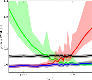
Figure 4: Performance statistics obtained over $100$ generated trajectories for $30$ different values of $\sigma_{\omega}$. We have compared the proposed filter $\text{SE}(2)^{2}$ (blue) and $\text{SE}(2)\times{\mathbb{R}}^{3}$ (orange) with the EKF based CTRV (green), KF based CV (red), and measurements (black), where the solid lines corresponds to mean values, while transparent areas correspond to one standard deviation (in both $+/-$ directions) of each of the associated RMSEs. We can notice that the $\text{SE}(2)\times{\mathbb{R}}^{3}$ and $\text{SE}(2)^{2}$ filters, whose difference is barely noticable, exhibit similar behaviour, outperforming the other two filters.

V Conclusion

In this paper we have proposed novel models for tracking a moving object exploiting its motion on the rigid body motion group $\text{SE}(2)$. The proposed filtering approach relied on the extended Kalman filter for matrix Lie groups, since the rigid body motion group itself is a matrix Lie group. Therefore, we have modeled the state space as either a direct product of the of the $\text{SE}(2)$ group and the ${\mathbb{R}}^{3}$ vector, i.e., $\text{SE}(2)\times{\mathbb{R}}^{3}$, or two $\text{SE}(2)$ groups, i.e. $\text{SE}(2)\times\text{SE}(2)$, where the first term described the current pose, while the second term handled second order dynamics. We have analyzed the performance of the proposed filters on a large number of synthetic trajectories and compared them to (i) the EKF based constant velocity and turn rate and (ii) the KF based constant velocity models. The $\text{SE}(2)\times{\mathbb{R}}^{3}$ and $\text{SE}(2)^{2}$ filters showed similar performance on the synthetic dataset, and have significantly outperformed other well-established approaches for a wide range of intensities in the rotation component.

Even though the presented work was applied on a tracking problem, we believe it can serve as a starting point for further exploitation of estimation on matrix Lie groups and its applications on different problems. The use of higher order dynamics may be of special interest for the domain of robotics, as well as for multi-target tracking applications. Furthermore, these techniques could also find application in other rigid body motion estimation problems requiring precise pose estimation and higher-order motion.

References

• [1] T. D. Barfoot and P. T. Furgale, “Associating Uncertainty With Three-Dimensional Poses for Use in Estimation Problems,” IEEE Transactions on Robotics, vol. 30, no. 3, pp. 679–693, Jun. 2014.
• [2] C. Hertzberg, R. Wagner, U. Frese, and L. Schröder, “Integrating Generic Sensor Fusion Algorithms with Sound State Representations through Encapsulation of Manifolds,” Information Fusion, vol. 14, no. 1, pp. 57–77, Jul. 2013.
• [3] R. M. Murray, Z. Li, and S. S. Sastry, A Mathematical Introduction to Robotic Manipulation.   CRC Press, 1994, vol. 29.
• [4] F. C. Park, J. E. Bobrow, and S. R. Ploen, “A Lie Group Formulation of Robot Dynamics,” The International Journal of Robotics Research, vol. 14, no. 6, pp. 609–618, 1995.
• [5] A. J. Davison, “Real-time simultaneous localisation and mapping with a single camera,” in International Conference on Computer Vision (ICCV), vol. 2.   IEEE, 2003, pp. 1403–1410.
• [6] Y. M. Lui, “Advances in matrix manifolds for computer vision,” Image and Vision Computing, vol. 30, no. 6-7, pp. 380–388, Jun. 2012.
• [7] S.-F. Su and C. S. G. Lee, “Manipulation and propagation of uncertainty and verification of applicability of actions in assembly tasks,” IEEE Transactions on Systems, Man, and Cybernetics, vol. 22, no. 6, pp. 1376–1389, 1992.
• [8] G. Silveira, E. Malis, and P. Rives, “An Efficient Direct Approach to Visual SLAM,” IEEE Transactions on Robotics, vol. 24, no. 5, pp. 969–979, 2008.
• [9] W. Park, Y. Wang, and G. S. Chirikjian, “The Path-of-Probability Algorithm for Steering and Feedback Control of Flexible Needles,” The International Journal of Robotics Research, vol. 29, no. 7, pp. 813–830, 2010.
• [10] R. A. Srivatsan, M. Travers, and H. Choset, “Using Lie algebra for shape estimation of medical snake robots,” in International Conference on Intelligent Robots and Systems (IROS), Chicago, USA, 2014.
• [11] A. W. Long, K. C. Wolfe, M. J. Mashner, and G. S. Chirikjian, “The Banana Distribution is Gaussian : A Localization Study with Exponential Coordinates,” in Proceedings of Robotics: Science and Systems (RSS), 2012.
• [12] M. Agrawal, “A lie algebraic approach for consistent pose registration for general euclidean motion,” in International Conference on Intelligent Robots and Systems (IROS).   IEEE, 2006, pp. 1891–1897.
• [13] S. Thrun, W. Burgard, and D. Fox, Probabilistic Robotics.   MIT Press, 2006.
• [14] G. Kurz, I. Gilitschenski, and U. D. Hanebeck, “The partially wrapped normal distribution for SE(2) estimation,” in International Conference on Multisensor Fusion and Information Integration for Intelligent Systems (MFI), 2014.
• [15] I. Gilitschenski, G. Kurz, S. J. Julier, and U. D. Hanebeck, “A New Probability Distribution for Simultaneous Representation of Uncertain Position and Orientation,” in International Conference on Information Fusion (FUSION), 2014.
• [16] G. Bourmaud, R. Mégret, M. Arnaudon, and A. Giremus, “Continuous-Discrete Extended Kalman Filter on Matrix Lie Groups Using Concentrated Gaussian Distributions,” Journal of Mathematical Imaging and Vision, vol. 51, no. 1, pp. 209–228, 2015.
• [17] Y. Bar-Shalom, T. Kirubarajan, and X.-R. Li, Estimation with Applications to Tracking and Navigation.   John Wiley & Sons, Inc., 2002.
• [18] R. Schubert, “Evaluating the utility of driving: Toward automated decision making under uncertainty,” IEEE Transactions on Intelligent Transportation Systems, vol. 13, no. 1, pp. 354–364, 2012.
• [19] R. Siegwart and I. R. Nourbakhsh, Introduction to Autonomous Mobile Robots.   Scituate, MA, USA: Bradford Company, 2004.
• [20] G. S. Chirikjian, Stochastic Models, Information Theory, and Lie Groups, Volume 2: Analytic Methods and Modern Applications.   Springer, 2012.
• [21] Y. Wang and G. S. Chirikjian, “Nonparametric Second-Order Theory of Error Propagation on Motion Groups,” International Journal on Robotic Research, vol. 27, no. 11, pp. 1258–1273, 2008.
• [22] K. C. Wolfe, M. Mashner, and G. S. Chirikjian, “Bayesian Fusion on Lie Groups,” Journal of Algebraic Statistics, vol. 2, no. 1, pp. 75–97, 2011.
• [23] G. Bourmaud, R. Mégret, A. Giremus, and Y. Berthoumieu, “Discrete Extended Kalman Filter on Lie Groups,” in European Signal Processing Conference (EUSIPCO), 2013, pp. 1–5.
• [24] G. Chirikjian and M. Kobilarov, “Gaussian Approximation of Non-linear Measurement Models on Lie Groups .” in Conference on Decision and Control (CDC).   IEEE, 2014, pp. 6401–6406.