On Input Design for Regularized LTI System Identification: Power-constrained Input

Abstract

Input design is an important issue for classical system identification methods but has not been investigated for the kernel-based regularization method (KRM) until very recently. In this paper, we consider in the time domain the input design problem of KRMs for LTI system identification. Different from the recent result, we adopt a Bayesian perspective and in particular make use of scalar measures (e.g., the $A$-optimality, $D$-optimality, and $E$-optimality) of the Bayesian mean square error matrix as the design criteria subject to power-constraint on the input. Instead to solve the optimization problem directly, we propose a two-step procedure. In the first step, by making suitable assumptions on the unknown input, we construct a quadratic map (transformation) of the input such that the transformed input design problems are convex, the number of optimization variables is independent of the number of input data, and their global minima can be found efficiently by applying well-developed convex optimization software packages. In the second step, we derive the expression of the optimal input based on the global minima found in the first step by solving the inverse image of the quadratic map. In addition, we derive analytic results for some special types of fixed kernels, which provide insights on the input design and also its dependence on the kernel structure.

and

1 Introduction

Over the past few years, the kerel-based regularization method (KRM), which was first introduced in Pillonetto & De Nicolao (2010) and then further developed in Pillonetto et al. (2011); Chen et al. (2012, 2014), has received increasing attention in the system identification community, see e.g., Pillonetto et al. (2014); Chiuso (2016) and the references therein. It has become a complement to the classical maximum likelihood/prediction error methods (ML/PEM),Ljung (1999); Söderström & Stoica (1989), which can be justified in a couple of aspects. First, the kernel, through which the regularization is defined, provides a carrier for prior knowledge on the dynamic system to be identified. Second, the model complexity is tuned in a continuous manner through the hyperparameter, which is the parameter vector used to parameterize the kernel, Pillonetto & Chiuso (2015); Mu et al. (2017). Third, extensive simulation results show that KRM can have better average accuracy and robustness than ML/PEM for the data that is short and/or has low signal-to-noise ratio, Chen et al. (2012); Pillonetto et al. (2014), and as a result, algorithms of KRM have been added to the System Identification Toolbox of MATLAB (Ljung et al., 2015).

Most of the recent progress for KRM focus on the issues of kernel design and hyperparameter estimation. For the former issue, many kernels have been proposed and analyzed to embed various kinds of prior knowledge, Chen et al. (2016); Chen & Ljung (2017); Carli et al. (2017); Marconato et al. (2016); Zorzi & Chiuso (2017); Pillonetto et al. (2016). In particular, two systematic ways are introduced to design kernels in Chen & Ljung (2017): one is from a machine learning perspective which treats the impulse response as a function, and the other one is from a system theory perspective which associates the impulse response with a linear time-invariant (LTI) system. In Zorzi & Chiuso (2017), a harmonic analysis is first provided for existing kernels including the amplitude modulated locally stationary (AMLS) kernel introduced in Chen & Ljung (2017) and then is shown to be a useful tool to design more general kernels. In contrast, there are few results reported for the issue of hyperparameter estimation Pillonetto & Chiuso (2015); Mu et al. (2017). In particular, it was shown in Mu et al. (2017) that the Stein’s unbiased risk estimator (SURE) is asymptotically optimal but the widely used empirical Bayes estimator is not.

There are some issues for KRM that have not been addressed adequately including the issue of input design. There are numerous results on this issue for ML/PEM, see e.g., the survey papers (Mehra, 1974; Hjalmarsson, 2005; Gevers, 2005) and the books (Goodwin & Payne, 1977; Ljung, 1999; Zarrop, 1979). The current state-of-the-art of input design for ML/PEM, see e.g., Jansson & Hjalmarsson (2005); Hildebrand & Gevers (2003); Hjalmarsson (2009), is to solve the problem in a two-step procedure. The first step is to pose the problem in the frequency domain as a convex optimization problem with a linear matrix inequality constraint and then derive the optimal input power spectrum with respect to certain design criteria, and the second step is to derive the realization of the input corresponding to the optimal power spectrum. The typical design criteria are scalar measures (e.g., the trace, the determinant or the largest eigenvalue) of the asymptotic covariance matrix of the parameter estimate or the information matrix of ML/PEM subject to various constrains on the inputs (e.g., energy or amplitude constraints). The typical realization of the input is the filtered white noise by spectral factorization of the desired input spectrum (Jansson & Hjalmarsson, 2005; Hjalmarsson, 2009) or a multisine signal (Hildebrand & Gevers, 2003). In contrast, there have been no results reported on this issue for KRM until very recently in Fujimoto & Sugie (2016), where for a fixed kernel (a kernel with fixed hyperparameter), the optimal input is derived by maximizing the mutual information between the output and the impulse response subject to energy-constraint on the input. The proposed method in Fujimoto & Sugie (2016) is very interesting but the number of the optimization variables induced by the input design problem is equal to the number of data and thus is expensive to solve when the number of data is large. Moreover, the induced optimization problem is nonconvex and the proposed gradient-based algorithm may be inefficient and subject to local minima issue. Nevertheless, their simulation result looks quite promising and motivates the interest of further investigation.

In this paper, we treat the input design problem for KRM from a perspective different from Fujimoto & Sugie (2016). Similar to Fujimoto & Sugie (2016), we also assume that the kernel is fixed (otherwise, it can be estimated from a preliminary experiment), but our starting point is different and is the mean square error (MSE) matrix of the regularized finite impulse response (FIR) estimate Chen et al. (2012). Since the MSE matrix depends on the unknown true impulse response, we propose to make use of the Bayesian interpretation of the KRM and derive the so-called Bayesian MSE matrix, which only depends on the fixed kernel and the input. It is then possible to use scalar measures of the Bayesian MSE matrix as the design criteria to optimize the input, e.g., the $A$-optimality, $D$-optimality, and $E$-optimality measures. Interestingly, the design criterion in Fujimoto & Sugie (2016) is equivalent to the $D$-optimality of the Bayesian MSE matrix introduced here. Moreover, we also treat the unknown input in a way different from Fujimoto & Sugie (2016) and consider power-constrained input Goodwin & Payne (1977) accordingly.

Instead to solve the optimization problem induced by the input design in a direct way, we propose a two-step procedure. In the first step, under the assumption on the unknown input, we construct a quadratic map (transformation) of the input such that the transformed input design problems are convex, the number of optimization variables is equal to the order of the FIR model, and their global minima can be found efficiently by applying well-developed convex optimization software packages, such as CVX (Grant & Boyd, 2016). In the second step, we derive the expression of the optimal input based on the global minima found in the first step by solving the inverse image of the quadratic map. From an optimization point of view, a similar optimization problem to the underlying one of our method appeared before in Hildebrand & Gevers (2003); Jansson & Hjalmarsson (2005). However, our method is essentially different. First, our input design problem is posed and solved in the time domain. Second, our method is not based on asymptotic theory and works for any finite number of data. Third, the optimal input is derived by solving the inverse image of the quadratic map. In addition, we derive analytic results for some special types of fixed kernels, which provide insights on input design and also its dependence on the kernel structure. In particular, we show that the impulsive input is globally optimal and the white noise input is asymptotically globally optimal for all diagonal kernels, but they are often not optimal for kernels with correlation, e.g, the diagonal correlated (DC) kernel introduced in Chen et al. (2012). Finally, numerical simulation results are provided to illustrate the efficacy of our method.

The remaining parts of this paper are organized as follows. In Section 2, we first review briefly KRM. In Section 3, we state the problem formulation of the input design problem. In Section 4, we introduce the two-step procedure to solve the input design problem. Then we show in Section 5 that for some fixed kernels, it is possible to derive the explicit solution of the optimal input. The numerical simulation is given in Section 6 to demonstrate the proposed method. Finally, we conclude the paper in Section 7. All proofs of Theorems, Propositions, and Lemmas are postponed to the Appendix.

2 Regularized FIR Model Estimation

Consider a single-input single-output linear stable and causal discrete-time system

$$y(t)=G_{0}(q^{-1})u(t)+v(t).$$ (1)

Here $t\in\mathbb{N}$ is the time index, $q^{-1}$ is the backshift operator ($q^{-1}u(t)=u(t-1)$), $y(t),u(t)\in\mathbb{R}$ are the output and input of the system at time $t$, respectively, $v(t)\in\mathbb{R}$ is a zero mean white noise with variance $\sigma^{2}>0$ and is independent of the input $u(t)$, and the transfer function $G_{0}(q^{-1})$ of the “true” system is

$$G_{0}(q^{-1})=\sum_{k=1}^{\infty}g_{k}^{0}q^{-k},$$ (2)

where the coefficients $g_{k}^{0}\in\mathbb{R},k=1,\cdots,\infty$ form the impulse response of the system. Further, we assume that the input $u(t)$ is known (deterministic). The system identification problem is to estimate a model of $G_{0}(q^{-1})$ as well as possible based on the data $\{u(t-1),y(t)\}_{t=1}^{N}$.

The stability of $G_{0}(q^{-1})$ implies that its impulse response decays to zero, and thus it is always possible to truncate the infinite impulse response by a high order finite impulse response (FIR) model:

$$G(q^{-1})=\sum_{k=1}^{n}g_{k}q^{-k},~{}~{}\theta=[g_{1},\cdots,g_{n}]^{T}\in\mathbb{R}^{n},$$ (3)

where $n$ is the order of the FIR model and $(\cdot)^{T}$ denotes the transpose of a matrix or vector. With the FIR model (3), system (1) is written as

$$y(t)\!=\!\phi^{T}\!(t)\theta\!+\!v(t),~{}\phi(t)\!=\![u(t\!-\!1),\cdots,u(t\!-\!n)]^{T},$$ (4)

and its matrix-vector form is

$$\hskip 30.00005ptY=\Phi\theta+V,$$ (5)

$$Y=[y(1)~{}y(2)\cdots~{}y(N)]^{T},$$ (6)

$$\Phi=[\phi(1)~{}\phi(2)~{}\cdots~{}\phi(N)]^{T},$$ (7)

$$V=[v(1)~{}v(2)~{}\cdots~{}v(N)]^{T},$$ (8)

where the unknown input $u(t)$ with $t=-1,\dots,-n+1$, can be handled in different ways: e.g., they can be not used (“non-windowed”) or they can be set to zero (“pre-windowed”); see (Ljung, 1999, p. 320) for discussions.

There are different methods to estimate $\theta$ and the simplest one is perhaps the least squares (LS) method:

$$\widehat{\theta}_{N}^{\rm LS}=\operatorname*{arg\,min}_{\theta}\|Y-\Phi\theta\|^{2}=(\Phi^{T}\Phi)^{-1}\Phi^{T}Y,$$ (9)

where $\|\cdot\|$ is the Euclidean norm. However, $\widehat{\theta}_{N}^{\rm LS}$ may have large variance and thus large mean square error (MSE), as its variance increases approximately linearly with respect to $n$. One way to mitigate the possible large variance and reduce the MSE is by using the regularized least squares (RLS) method, see e.g., Chen et al. (2012):

$$\widehat{\theta}_{N}^{\rm R}= \operatorname*{arg\,min}_{\theta\in\mathbb{R}^{n}}\|Y-\Phi\theta\|^{2}+\sigma^{2}\theta^{T}P^{-1}\theta$$ (10a)

$$= P\Phi^{T}(\Phi P\Phi^{T}+\sigma^{2}I_{N})^{-1}Y,$$ (10b)

where $P$ is positive semidefinite and is called the kernel matrix ($\sigma^{2}P^{-1}$ is often called the regularization matrix), and $I_{N}$ is the $N$-dimensional identity matrix.

Now we let $\theta_{0}=[g_{1}^{0},\cdots,g_{n}^{0}]^{T}$, where $g_{1}^{0},\dots,g_{n}^{0}$ are defined in (2) and we then obtain the MSE matrix of $\widehat{\theta}_{N}^{\rm R}$:

$$\widehat{\theta}^{\rm R}_{N} -\theta_{0}=-\sigma^{2}Q^{-1}P^{-1}\theta_{0}+Q^{-1}\Phi^{T}V,$$ (11)

$$M_{N} =\mathrm{E}(\widehat{\theta}_{N}^{\rm R}-\theta_{0})(\widehat{\theta}_{N}^{\rm R}-\theta_{0})^{T}$$

$$=\sigma^{4}Q^{-1}P^{-1}\theta_{0}\theta_{0}^{T}P^{-1}Q^{-1}\!+\!\sigma^{2}Q^{-1}\Phi^{T}\Phi Q^{-1}$$ (12)

$$Q =\Phi^{T}\Phi+\sigma^{2}P^{-1},$$ (13)

where $\rm E(\cdot)$ is the mathematical expectation. It has been shown in Mu et al. (2017, Prop. 2) that for a suitably chosen kernel matrix $P$, $\operatorname*{Tr}(M_{N}(\widehat{\theta}_{N}^{\rm R}))\leq\operatorname*{Tr}(M_{N}(\widehat{\theta}_{N}^{\rm LS}))$, where $\operatorname*{Tr}(\cdot)$ is the trace of a square matrix.

The problem to achieve a good $\widehat{\theta}^{\rm R}_{N}$ boils down to the choice of a suitable kernel matrix $P$, which contains two issues: kernel design and hyperparameter estimation.

2.1 Kernel Design

The issue of kernel design is regarding how to embed in a kernel the prior knowledge of the underlying system to be identified by parameterizing the kernel with a parameter vector, say $\eta$, called hyperparameter. The essence of kernel design is analogous to the model structure design for ML/PEM, and the kernel determines the underlying model structure for the regularized FIR model (10b). So far, several kernels have been proposed, such as the stable spline (SS) kernel (Pillonetto & De Nicolao, 2010), the diagonal correlated (DC) kernel and the tuned-correlated (TC) kernel (Chen et al., 2012), the latter two of which are defined as follows:

$${\rm DC}:~{}~{}P_{kj}(\eta)=c\lambda^{(k+j)/2}\rho^{|j-k|},$$

$$~{}~{}\eta=[c,\lambda,\rho]\in\Omega=\{c\geq 0,0\leq\lambda\leq 1,|\rho|\leq 1\};$$ (14)

$${\rm TC}:~{}~{}P_{kj}(\eta)=c\lambda^{\max(k,j)},$$

$$~{}~{}~{}~{}~{}~{}~{}\eta=[c,\lambda]\in\Omega=\{c\geq 0,0\leq\lambda\leq 1\}.$$ (15)

where the TC kernel (15) is a special case of the DC kernel with $\rho=\sqrt{\lambda}$ (Chen et al., 2012) and is also called the first order SS kernel (Pillonetto et al., 2014).

2.2 Hyperparameter Estimation

Once a kernel is designed, the next step is to determine the hyperparameter based on the data. The essence of hyperparameter estimation is analogous to the model order selection for ML/PEM, and the hyperparameter determines the model complexity of the regularized FIR model (10b). Several estimation methods have been suggested in (Pillonetto et al., 2014, Section 14). The most widely used method is the empirical Bayes (also called marginal likelihood maximization) method. The idea is to adopt the Bayesian perspective and embed the regularization term $\sigma^{2}\theta^{T}P^{-1}\theta$ in a Bayesian framework. More specifically, we assume in (4) that $v(t)$ and $\theta$ are independent and Gaussian distributed with $v(t)\sim\mathscr{N}(0,\sigma^{2})$ and

$$\theta\sim\mathscr{N}(0,P).$$ (16)

Then $\theta$ and $Y$ are jointly Gaussian distributed and moreover, the posterior distribution of $\theta$ given $Y$ is

$$\theta|Y\sim\mathscr{N}(\widehat{\theta}^{\rm R},\widehat{P}^{\rm R}),$$

$$\widehat{\theta}^{\rm R}_{N}=P\Phi^{T}(\Phi P\Phi^{T}+\sigma^{2}I_{N})^{-1}Y,$$

$$\widehat{P}^{\rm R}_{N}=P-P\Phi^{T}(\Phi P\Phi^{T}+\sigma^{2}I_{N})^{-1}\Phi P=\sigma^{2}Q^{-1}.$$ (17)

Moreover, the output $Y$ is also Gaussian with zero mean and covariance matrix $\Phi P(\eta)\Phi^{T}+\sigma^{2}I_{N}$. Therefore, the hyperparameter $\eta$ can be estimated by maximizing the marginal likelihood, or equivalently,

$$\text{EB: }\ \widehat{\eta} =\operatorname*{arg\,min}_{\eta\in\Omega}Y^{T}F(\eta)^{-1}Y+\log\det(F(\eta)),$$ (18)

$$F =\Phi^{T}P\Phi+\sigma^{2}I_{N},$$ (19)

where $\det(\cdot)$ is the determinant of a matrix. The EB (18) has the advantage that it is robust Pillonetto & Chiuso (2015), but not asymptotical optimal in the sense of MSE (Mu et al., 2017).

3 Problem Formulation for Input Design

3.1 Bayesian MSE Matrix and Design Criteria

The goal of input design is to determine, under suitable conditions, an input sequence such that the regularized FIR model (10b) is as good as possible. The MSE matrix (12) is a natural measure to evaluate how good the regularized FIR model estimate (10b) is. Unfortunately, the first term of (12) depends on the true impulse response $\theta_{0}$ and thus it can not be used directly.

There are different ways to deal with this difficulty. We adopt a Bayesian perspective that is similar to the derivation of (18). More specifically, we assume that

$$\theta_{0}\sim\mathscr{N}(0,P).$$ (20)

Then taking expectation on both side of (12) leads to

$$M_{N} =\sigma^{4}Q^{-1}P^{-1}Q^{-1}+\sigma^{2}Q^{-1}\Phi^{T}\Phi Q^{-1}$$

$$=\sigma^{2}Q^{-1}(\sigma^{2}P^{-1}+\Phi^{T}\Phi)Q^{-1}$$

$$=\sigma^{2}Q^{-1},\text{\ ``Bayesian MSE''}.$$ (21)

Since the Bayesian perspective is adopted, (21) is called the Bayesian MSE matrix of the regularized FIR model estimate (10b) under the assumption (20). Interestingly, the Bayesian MSE matrix (21) is equal to the posterior covariance of the regularized FIR model estimate (17) under the assumption (16).

We will tackle the input design problem by minimizing a scalar measure of the Bayesian MSE matrix (21) of the regularized FIR model estimate (10b). This idea is similar to that of the traditional input design problem by minimizing a scalar measure of the asymptotic covariance matrix of the parameter estimate (Ljung, 1999). The typical $A$-optimality, $D$-optimality, and $E$-optimality scalar measures of the Bayesian MSE matrix (21) will be chosen as the design criteria for the input design problem and given below:

$$D-\mbox{optimality}:~{}~{}\det(M_{N})\displaystyle\stackrel{{\scriptstyle\triangle}}{{=}}\det(\sigma^{2}Q^{-1}),$$ (22)

$$A-\mbox{optimality}:~{}~{}{\rm Tr}(M_{N})\displaystyle\stackrel{{\scriptstyle\triangle}}{{=}}{\rm Tr}(\sigma^{2}Q^{-1}),$$ (23)

$$E-\mbox{optimality}:~{}~{}\lambda_{\rm max}(M_{N})\displaystyle\stackrel{{\scriptstyle\triangle}}{{=}}\lambda_{\rm max}(\sigma^{2}Q^{-1}),$$ (24)

where $\lambda_{\rm max}(\cdot)$ is the largest eigenvalue of a matrix.

Remark 1.

Another possible way to deal with the unknown $\theta_{0}$ in the MSE matrix (12) is to replace $\theta_{0}$ by an estimate obtained in advance, for example, the LS estimate (9). In this case, the MSE matrix (12) becomes

$$\sigma^{4}Q^{-1}P^{-1}\widehat{\theta}_{N}^{\rm LS}(\widehat{\theta}_{N}^{\rm LS})^{T}P^{-1}Q^{-1}+\sigma^{2}R^{-1}\Phi^{T}\Phi Q^{-1}.$$ (25)

Clearly, the input design would depend on the quality of the chosen estimate.

Remark 2.

Interestingly, the $D$-optimality measure (22) is equivalent to the mutual information between the true impulse response and the output $Y$ given in Fujimoto & Sugie (2016).

3.2 Problem Statement

Now we are able to state the input design problem based on the design criteria (22)–(24).

Assume that the kernel matrix $P(\eta)$ and the variance $\sigma^{2}$ of the noise are known in advance (otherwise, they can be estimated with a preliminary experiment) and also note that the construction of the regression matrix $\Phi$ in (7) requires the inputs $u_{-n+1},\cdots,u_{N-1}$. Then the input design problem is to determine an input sequence

$$u_{-n+1},\cdots,u_{-1},u_{0},u_{1},\cdots,u_{N-1},$$ (26)

where, for simplicity, $u_{t}$ is used to denote $u(t)$ hereafter, such that the input sequence (26) minimizes the design criteria (22)–(24) subject to certain constraints.

It should be noted that the inputs $u_{-n+1},\cdots,u_{-1}$ are unknown for the identification problem but can be treated as design variables for the input design problem. In particular, Fujimoto & Sugie (2016) sets the inputs $u_{-n+1},\cdots,u_{-1}$ to be zero, i.e.,

$$u_{-n+1}=\cdots=u_{-1}=0,$$ (27)

and essentially minimizes the $D$-optimality measure (22) subject to an energy-constraint

$$\mathcal{U} =\{u|u^{T}u\leq\mathscr{E},u\in\mathbb{R}^{N}\},$$ (28)

$$u =[u_{0},u_{1},\cdots,u_{N-1}]^{T},$$

where $\mathscr{E}>0$ is a known constant and is the maximum available energy for the input.

Here, we treat $u_{-n+1},\cdots,u_{-1}$ in a different way. Our idea is not only to reduce the number of optimization variables of the input design problem, but also to bring it certain structure such that it becomes easier to solve, see Section 4 for details. In particular, we assume $N\geq n$ and set

$$u_{-i} =u_{N-i},\quad i=1,\cdots,n-1.$$ (29)

The advantage of doing so is that the regression matrix $\Phi$ has a good structure and becomes a circulant matrix:

$$\Phi=\left[\begin{array}[]{cccccc}u_{0}&u_{N-1}&\cdots&u_{N-n+2}&u_{N-n+1}\\ u_{1}&u_{0}&\cdots&u_{N-n+3}&u_{N-n+2}\\ \vdots&\vdots&\ddots&\vdots&\vdots\\ u_{n-2}&u_{n-3}&\cdots&u_{0}&u_{N-1}\\ u_{n-1}&u_{n-2}&\cdots&u_{1}&u_{0}\\ u_{n}&u_{n-1}&\cdots&u_{2}&u_{1}\\ \vdots&\vdots&\ddots&\vdots&\vdots\\ u_{N-1}&u_{N-2}&\cdots&u_{N-n+1}&u_{N-n}\end{array}\right].$$

Moreover, we consider the power constraint on the input sequence (26) used for the traditional ML/PEM input design problem, see e.g., (Goodwin & Payne, 1977, p. 129, eq. (6.3.12)), i.e.,

$$\sum_{t=1}^{N}u_{t-i}^{2}=\mathscr{E},\ i=1,\dots,n,$$ (30)

Under the assumption (29), the input design problem of minimizing the design criteria (22)–(24) subject to the constraint (30) can be equivalently written as follows:

$$u^{*}_{\rm D}\displaystyle\stackrel{{\scriptstyle\triangle}}{{=}}\arg\min_{u\in\mathscr{U}}{\rm\det}(\sigma^{2}Q^{-1}),$$ (31)

$$u^{*}_{\rm A}\displaystyle\stackrel{{\scriptstyle\triangle}}{{=}}\arg\min_{u\in\mathscr{U}}{\rm Tr}(\sigma^{2}Q^{-1}),$$ (32)

$$u^{*}_{\rm E}\displaystyle\stackrel{{\scriptstyle\triangle}}{{=}}\arg\min_{u\in\mathscr{U}}\lambda_{\rm max}(\sigma^{2}Q^{-1}),$$ (33)

where the constraint (30) under the assumption (29) becomes

$$\mathscr{U} =\{u|u^{T}u=\mathscr{E},u\in\mathbb{R}^{N}\},$$ (34)

$$u =[u_{0},u_{1},\cdots,u_{N-1}]^{T},$$

It is worth to note that the optimal input is not unique in general. To check this, note that if an input sequence $u^{*}$ is optimal, then $-u^{*}$ is also optimal, where $u^{*}$ can be any of $u^{*}_{\rm D},u^{*}_{\rm A}$ and $u^{*}_{\rm E}$. Therefore, $u^{*}_{\rm D},u^{*}_{\rm A},u^{*}_{\rm E}$ should be understood as the set of all optimal inputs minimizing (31), (32), (33), respectively.

4 Main Results

Similar to Fujimoto & Sugie (2016), we can also try to solve the input design problems (31)–(33) by using gradient-based algorithms. However, such algorithms may have the following problems:

1. the input design problems (31)–(33) is expensive to solve for large $N$, because the number of optimization variables is $N$.

2. the gradient-based algorithms may be subject to the issue of local minima, because the input design problems (31)–(33) are non-convex.

We propose to solve the input design problems (31)–(33) in a two-step procedure, and its idea is sketched below:

1. under the assumption (29), we construct a quadratic map (transformation) of $u$, say $f(u)$, such that the transformed input design problems of (31)–(33) are convex and thus can be solved efficiently.

2. by exploiting the properties of $f(\cdot)$ and based on the globally minima of the transformed input design problems of (31)–(33), we derive the optimal inputs by solving the inverse of the map $f(\cdot)$.

4.1 A Quadratic Map

Under the assumption (29), we define

$$r =[r_{0},r_{1},\cdots,r_{n-1}]^{T},$$ (35)

$$r_{j} =\sum_{k=0}^{N-1}u_{k}u_{k-j},\ j=0,\dots,n-1.$$

Then we have

$$R\displaystyle\stackrel{{\scriptstyle\triangle}}{{=}}\Phi^{T}\Phi=\left[\begin{array}[]{cccccc}r_{0}&r_{1}&\cdots&r_{n-2}&r_{n-1}\\ r_{1}&r_{0}&\ddots&r_{n-3}&r_{n-2}\\ \vdots&\ddots&\ddots&\ddots&\vdots\\ r_{n-2}&r_{n-3}&\ddots&r_{0}&r_{1}\\ r_{n-1}&r_{n-2}&\cdots&r_{1}&r_{0}\\ \end{array}\right],$$ (41)

which is a positive semidefinite Toeplitz matrix.

Actually, the definition (35) determines a quadratic vector-valued function

$$r=f(u)=[f_{0}(u),\cdots,f_{n-1}(u)]^{T}.$$ (42)

The domain of $f(\cdot)$ is $\mathscr{U}$ which has been defined in (34) and is convex and compact, and the $j$-element of $f(\cdot)$ is

$$f_{j}(u)=u^{T}L_{j}u,\ j=0,\dots,n-1,$$ (43)

$$L_{j}=\frac{1}{2}\left[\begin{array}[]{cc}0&I_{N-j}\\ I_{j}&0\end{array}\right]+\frac{1}{2}\left[\begin{array}[]{cc}0&I_{j}\\ I_{N-j}&0\end{array}\right].$$ (48)

It follows that the corresponding value $r_{0}$ is $\mathscr{E}$ for any input $u\in\mathscr{U}$. Moreover, denote the image of $f(\cdot)$ under $\mathscr{U}$ by

$$\mathscr{F}=\{f(u)|u\in\mathscr{U}\},$$ (49)

which is a convex polytope (See Theorem 8 below).

4.2 Transformed Input Design Problem

Interestingly, the quadratic map (42) makes the transformed input design problems of (31) to (33) convex.

To show this, note that the matrix $Q$ in (13) can be written as

$$Q(r)=r_{0}I_{n}+r_{1}Q_{1}+\cdots+r_{n-1}Q_{r-1}+\sigma^{2}P^{-1},$$ (50)

where $Q_{i}\in\mathbb{R}^{n\times n}$, $i=1,\dots,n-1$ is symmetric and zero everywhere except the $(jl)$-element which is one if $|j-l|=i$ with $j,l=1,\dots,n$. The map (42) transforms the input design problems (31)–(33) to the following optimization problems, respectively,

$$r^{*}_{\rm D}=\operatorname*{arg\,min}_{r\in\mathscr{F}}\log\det(\sigma^{2}Q(r)^{-1})$$ (51)

$$r^{*}_{\rm A}=\operatorname*{arg\,min}_{r\in\mathscr{F}}{\rm Tr}(\sigma^{2}Q(r)^{-1})$$ (52)

$$r^{*}_{\rm E}=\operatorname*{arg\,min}_{r\in\mathscr{F}}\lambda_{\rm max}(\sigma^{2}Q(r)^{-1})$$ (53)

where $\log\det(\cdot)$ is used instead of $\det(\cdot)$.

Proposition 3.

Consider the transformed input design problems (51) to (53). It follows that

• The problems (51) and (52) are strictly convex and thus $r^{*}_{\rm D}$ and $r^{*}_{\rm A}$ are unique in $\mathscr{F}$.

• The problem (53) is convex and $r^{*}_{\rm E}$ exists but may be not unique in $\mathscr{F}$.

Remark 4.

From an optimization point of view, the optimization problems (51) to (53), modulo the constraint, appeared before, see e.g., Jansson & Hjalmarsson (2005). However, the contexts are different: the elements of $r$ are the auto-correlation coefficients of the input power spectrum in Jansson & Hjalmarsson (2005) but they do not have such interpretation here unless we divide them by $N$ and let $N$ go to $\infty$. In addition, the positivity constraint of the input spectrum is transformed into a linear matrix inequality by applying the Kalman-Yakubovich-Popov lemma in Jansson & Hjalmarsson (2005), while the constraint here is the feasible set $\mathscr{F}$, which is a convex polytope (See Remark 9 below).

Remark 5.

An optimal $r^{*}$ satisfies $r_{0}^{*}=\mathscr{E}$, where $r_{0}^{*}$ is the first element of $r^{*}$, and $r^{*}$ could be $r^{*}_{\rm D}$ $r^{*}_{\rm A}$, and $r^{*}_{\rm E}$.

Remark 6.

For $i=1,\dots,n-1$, the elements of the gradient of (51) and (52) are respectively given by

$$\frac{\partial\log\det(\sigma^{2}Q(r)^{-1})}{\partial r_{i}}\!=\!-{\rm Tr}(Q(r)^{-1}Q_{i}),$$ (54)

$$\frac{\partial{\rm Tr}(\sigma^{2}Q(r)^{-1})}{\partial r_{i}}=-\sigma^{2}{\rm Tr}(Q(r)^{-2}Q_{i}).$$ (55)

4.3 Finding Optimal Inputs

Now we assume that the global minima of the transformed input design problems (51) to (53) have been found and denoted by $r^{*}\in\mathscr{F}$, which could be any one of $r^{*}_{\rm D},r^{*}_{\rm A},$ and $r^{*}_{\rm E}$. Then we consider the problem how to derive the optimal input $u^{*}$ from $r^{*}\in\mathscr{F}$ by exploiting the properties of the quadratic map $f(\cdot)$ and the inverse map of $f(\cdot)$ for a given vector $r\in\mathscr{F}$.

4.3.1 Properties of the Quadratic Map

The map $f(\cdot)$ has the following properties, which ease the derivation of the optimal input as will be seen shortly.

Theorem 7.

Consider the map $f(\cdot)$ defined in (42). Then there exists a matrix $S\in{\mathbb{R}}^{n\times N}$ and an orthogonal matrix $W\in{\mathbb{R}}^{N\times N}$ such that the map $f(\cdot)$ can be written in a composite form as follows:

$$f(u) =h_{1}(h_{2}(h_{3}(u)))~{}~{}\mbox{with}$$ (56)

$$h_{1}(x) =Sx$$ (57)

$$h_{2}(z) =[z_{0}^{2},z_{1}^{2},\cdots,z_{N-1}^{2}]^{T}$$ (58)

$$h_{3}(u) =W^{T}u$$ (59)

where $x=[x_{0},x_{1},\cdots,x_{N-1}]^{T}$, $z=[z_{0},z_{1},\cdots,z_{N-1}]^{T}$, Moreover, the image of $h_{3}(\cdot)$ is

$$\mathscr{Z}=\{h_{3}(u)|u\in\mathscr{U}\}=\{z|z^{T}z=\mathscr{E}\},$$

the image of $h_{2}(\cdot)$

$$\mathscr{X} =\{h_{2}(z)|z\in\mathscr{Z}\}$$ (60)

$$=\left\{x\Big{|}\sum_{i=0}^{N-1}x_{i}\!=\!\mathscr{E},x_{i}\geq 0,i\!=\!0,1,\dots,N\!-\!1\right\},$$ (61)

is a convex polytope and the image of $h_{1}(\cdot)$

$$\mathscr{F}=\{f(u)|u\in\mathscr{U}\}=\{Sx|x\in\mathscr{X}\}$$ (62)

is also a convex polytope.

One choice for the matrices $S$ and $W$ in Theorem 7 is given in the following theorem.

Theorem 8.

Let $\varpi=2\pi/N$ and define the vectors

$$\xi_{j}=\left[\begin{array}[]{c}1\\ \cos(j\varpi)\\ \cos(2j\varpi)\\ \vdots\\ \cos((N\!\!-\!1)j\varpi)\end{array}\right],~{}\zeta_{j}=\left[\begin{array}[]{c}0\\ \sin(j\varpi)\\ \sin(2j\varpi)\\ \vdots\\ \sin((N\!\!-\!1)j\varpi)\end{array}\right]$$

for $j=0,1,\dots$. Then, one choice for the matrices $W$ and $S$ in Theorem 7 is

1) when $N$ is even,

$$W\!=\!\sqrt{\frac{2}{N}}\left[\frac{\xi_{0}}{\sqrt{2}},\xi_{1},\cdots,\xi_{\frac{N-2}{2}},\frac{\xi_{\frac{N}{2}}}{\sqrt{2}},\zeta_{\frac{N-2}{2}},\cdots,\zeta_{1}\right]$$ (63)

$$S=\Big{[}\xi_{0},\xi_{1},\cdots,\xi_{n-1}\Big{]}^{T}$$

$$\hskip 6.00006pt=\left[\xi_{0}(1\!:\!n),\xi_{1}(1\!:\!n),\cdots,\xi_{\frac{N}{2}}(1\!:\!n),\cdots,\xi_{1}(1\!:\!n)\right]\!\!\!\!$$ (64)

and $\operatorname*{rank}(S)=\min(N/2\!+\!1,n)$. Also,

$$\mathscr{F}\!=\!\mathbf{conv}\left\{\mathscr{E}\xi_{0}(1\!:\!n),\mathscr{E}\xi_{1}(1\!:\!n),\cdots,\mathscr{E}\xi_{\frac{N}{2}}(1\!:\!n)\right\}$$ (65)

where $\mathbf{conv}\{\cdots\}$ is the convex hull of the corresponding vectors and $\xi_{j}(1\!:\!n)$ is the vector consisting of the first $n$ elements of $\xi_{j}$.

2) when $N$ is odd,

$$W=\sqrt{\frac{2}{N}}\left[\frac{\xi_{0}}{\sqrt{2}},\xi_{1},\cdots,\xi_{\frac{N-1}{2}},\zeta_{\frac{N-1}{2}},\cdots,\zeta_{1}\right]$$ (66)

$$S=\Big{[}\xi_{0},\xi_{1},\cdots,\xi_{n-1}\Big{]}^{T}$$

$$\hskip 6.99997pt=\left[\xi_{0}(1\!:\!n),\xi_{1}(1\!:\!n),\cdots,\xi_{\frac{N-1}{2}}(1\!:\!n),\right.$$

$$\hskip 70.0001pt\left.\xi_{\frac{N-1}{2}}(1\!:\!n),\cdots,\xi_{1}(1\!:\!n)\right]\!\!\!\!$$ (67)

and $\operatorname*{rank}(S)=\min((N\!+\!1)/2,n)$. In addition,

$$\mathscr{F}\!=\!\mathbf{conv}\left\{\mathscr{E}\xi_{0}(1\!:\!n),\mathscr{E}\xi_{1}(1\!:\!n),\cdots,\mathscr{E}\xi_{\frac{N\!-\!1}{2}}(1\!:\!n)\right\}.$$ (68)

Remark 9.

The transformed input design problems (51), (52), (53) can be solved effectively by CVX (Grant & Boyd, 2016). The optimization criteria of (51), (52), (53) are standard in CVX and we only need to rewrite the feasible set $\mathscr{F}$ as a number of linear equalities and inequalities by the definition of convex hull (65) or (68):

• when $N$ is even, we have from (65) that

  $$\begin{array}[]{l}\mathscr{E}S(:,1\!:\!N/2\!+\!1)a=r\\ a=[a_{1},a_{2},\cdots,a_{N/2+1}]^{T},\ a_{j}\geq 0\end{array}$$ (71)

  where $r\in\mathscr{F}$, $S(:,1\!:\!N/2\!+\!1)$ denotes the first $N/2\!+\!1$ columns of $S$, and the first equality constraint is $\sum_{j=1}^{N/2+1}a_{j}=1$ since the first element of $r$ is $\mathscr{E}$ and all the elements of the first row of $S$ are one.

• when $N$ is odd, we have from (68) that

  $$\begin{array}[]{l}\mathscr{E}S(:,1\!:\!(N\!+\!1)/2)a=r\\ a=[a_{1},a_{2},\cdots,a_{(N+1)/2}]^{T},\ a_{j}\geq 0.\end{array}$$ (74)

Since the columns of $S$ are symmetric (See (64) and (67)), $\mathscr{F}$ can be uniformly expressed by for even and odd $N$

$$\begin{array}[]{l}\mathscr{E}Sa=r\\ a=[a_{1},a_{2},\cdots,a_{N}]^{T},\ a_{j}\geq 0.\end{array}$$ (77)

4.3.2 Derivation of the Optimal Input

Given any $r\in\mathscr{F}$, the inverse image $f^{-1}(r)$ of $f(\cdot)$ can be derived in the following way based on (56)–(59):

1. we find the inverse image of $h_{1}(\cdot)$ for $r\in\mathscr{F}$:

   $$\mathscr{X}(r) \displaystyle\stackrel{{\scriptstyle\triangle}}{{=}}\left\{x|Sx=r,x\in\mathscr{X}\right\}$$

   $$=\{\mathscr{K}(S)\oplus S^{\dagger}r\}\cap\mathscr{X}$$ (78)

   where $S^{\dagger}$ is the Moore-Penrose pseudoinverse of $S$ and $\mathscr{K}(S)=\{x|Sx=0\}$ is the null space of $S$, and $\oplus$ is the direct sum between two subspace.

2. we find the inverse image of $h_{2}(\cdot)$ for $x\in\mathscr{X}(r)$:

   $$\mathscr{Z}(r) \!\displaystyle\stackrel{{\scriptstyle\triangle}}{{=}}\!\left\{z|h_{2}(z)\in\mathscr{X}(r)\right\}$$

   $$\!=\!\left\{[\pm\sqrt{x_{0}},\cdots,\pm\sqrt{x_{N-1}}]^{T}|x\in\mathscr{X}(r)\right\}.$$ (79)

3. we find the inverse image of $h_{3}(\cdot)$ for $z\in\mathscr{Z}(r)$:

   $$\mathscr{U}(r)\displaystyle\stackrel{{\scriptstyle\triangle}}{{=}}\left\{u|W^{T}u\in\mathscr{Z}(r)\right\}=\left\{Wz|z\in\mathscr{Z}(r)\right\}.$$ (80)

It is worth to note that $\mathscr{X}(r)$ is still a convex polytope.

Proposition 10.

The inverse image $\mathscr{X}(r)$ is a convex polytope and is determined by a group of halfspaces and hyperplanes:

$$\mathscr{X}(r)=\left\{x|Sx=r,x_{i}\geq 0,~{}i=0,\dots,N\!-\!1\right\}.$$ (81)

This means that the optimal inputs $u^{*}=\mathscr{U}(r^{*})$, where $u^{*}$ can be any of $u^{*}_{\rm D},u^{*}_{\rm A}$ and $u^{*}_{\rm E}$.

Remark 11.

Noting that $W$ is orthogonal and the row vectors of $S$ are part of the column vectors of $W$ subject to some scaling factors, a basis of $\mathscr{K}(S)$ can be derived as follows:

• when $N$ is even, a basis of $\mathscr{K}(S)$ is

  $$\left\{\begin{array}[]{ll}\{\zeta_{1},\cdots,\zeta_{\frac{N-2}{2}}\}&\mbox{if}~{}n\!-\!1\geq N/2,\\ \{\xi_{n},\cdots,\xi_{\frac{N}{2}},\zeta_{1},\cdots,\zeta_{\frac{N-2}{2}}\}&\mbox{if}~{}n\!-\!1<N/2.\end{array}\right.$$

• when $N$ is odd, a basis of $\mathscr{K}(S)$ is

  $$\left\{\begin{array}[]{ll}\{\zeta_{1},\cdots,\zeta_{\frac{N-1}{2}}\}&\mbox{if}~{}n\!-\!1\geq(N\!-\!1)/2,\\ \{\xi_{n},\cdots,\xi_{\frac{N\!-\!1}{2}},\zeta_{1},\cdots,\zeta_{\frac{N-2}{2}}\}&\mbox{if}~{}n\!-\!1<(N\!-\!1)/2.\end{array}\right.$$

Remark 12.

As can be seen from the algorithm given above for finding the optimal inputs $u^{*}$ from $r^{*}\in\mathscr{F}$, the key is to determine the set $\mathscr{X}(r^{*})$ while steps 2) and 3) are straightforward. Actually, some elements belonging to $\mathscr{X}(r^{*})$ can be derived from the global minima of the optimization problems (51)–(53). Assume that the global minima corresponding to the constraints (71) is $\{r^{*},a^{*}\}$, respectively, where $a^{*}=[a_{1}^{*},a_{2}^{*},\cdots,a_{N/2+1}^{*}]^{T}$. Then all vectors

$$\mathscr{E}\Big{[}a_{1}^{*},\alpha_{2}a_{2}^{*},\cdots,\alpha_{\frac{N}{2}}a_{\frac{N}{2}}^{*},a_{\frac{N}{2}\!+\!1}^{*},(1-\alpha_{\frac{N}{2}})a_{\frac{N}{2}}^{*},\cdots,(1-\alpha_{2})a_{2}^{*}\Big{]}^{T}$$

belong to $\mathscr{X}(r^{*})$ for $0\leq\alpha_{i}\leq 1,i=2,\cdots,N/2$. Accordingly, for the constraint (74) with $a^{*}=[a_{1}^{*},a_{2}^{*},\cdots,a_{\frac{N+1}{2}}^{*}]^{T}$, we have all vectors

$$\mathscr{E}\Big{[}a_{1}^{*},\alpha_{2}a_{2}^{*},\cdots,\alpha_{\frac{N+1}{2}}a_{\frac{N+1}{2}}^{*},(1-\alpha_{\frac{N+1}{2}})a_{\frac{N+1}{2}}^{*},\cdots,(1-\alpha_{2})a_{2}^{*}\Big{]}^{T}$$

belong to $\mathscr{X}(r^{*})$ for $0\leq\alpha_{i}\leq 1,i=2,\cdots,(N\!+\!1)/2$. At last, for the constraint (77) with $a^{*}=[a_{1}^{*},a_{2}^{*},\cdots,a_{N}^{*}]^{T}$, we have the vector $\mathscr{E}a^{*}$ belongs to $\mathscr{X}(r^{*})$.

5 Optimal Input for Some Special Cases

In general, there is no analytic solution to the input design problems. In this section, we study the optimal input for some special types of fixed kernels. The obtained analytic results provide insights on input design and also its dependence on the kernel structure.

5.1 Diagonal Kernel Matrices

We first consider the ridge kernel matrix and then more general diagonal kernel matrices.

5.1.1 Ridge Kernel Matrix

When the kernel matrix is

$$P=cI_{n},~{}\mbox{with}~{}c>0,$$ (82)

it is possible to obtain the explicit expression of $r^{*}_{\rm D}$ and $r^{*}_{\rm A}$, which is given in the following proposition.

Proposition 13.

Consider the ridge kernel matrix (82). Then we have

$$r^{*}_{\rm D}=r^{*}_{\rm A}=[\mathscr{E},\underbrace{0,\cdots,0}_{n-1~{}\mbox{\rm zeros}}]^{T}\displaystyle\stackrel{{\scriptstyle\triangle}}{{=}}r^{\dagger}.$$ (83)

Proposition 13 shows that for ridge kernel matrix (82), any input such that $\Phi^{T}\Phi=\mathscr{E}I_{n}$ is the global minimum of (31) and (32). The optimal input given in Proposition 13 is identical with the classic result of input design for FIR model estimation with ML/PEM given in Goodwin & Payne (1977). In fact, this result is not surprising since the ridge kernel assumes that the prior distribution of the true impulse response is independent and identically distributed Gaussian, which does not provide any information on the correlation and the decay rate of the true impulse response. The optimal solution (83) implies that the optimal inputs could be:

1. Impulsive inputs: $[\pm\sqrt{\mathscr{E}},0,\cdots,0]^{T}$;

2. White noise inputs as $N\rightarrow\infty$.

Note that the impulsive input is globally optimal since it satisfies (83) exactly. In contrast, it was only shown in Fujimoto & Sugie (2016) that the impulsive input is locally optimal. In addition, as $N\rightarrow\infty$, the white noise input is also globally optimal. Clearly, the white noise input is approximately globally optimal for large $N$.

5.1.2 General Diagonal Kernel Matrices

When the kernel matrix is

$$P=\mathrm{diag}([\lambda_{1},\lambda_{2},\cdots,\lambda_{n}])$$ (84)

where $\lambda_{i}>0$, $i=1,\dots,n$, and $\mathrm{diag}(\cdot)$ represents a diagonal matrix, the optimal $r^{*}_{\rm D}$ and $r^{*}_{\rm A}$ are same as the one in Proposition 13.

Theorem 14.

Consider the diagonal kernel matrix (84). Then we have

$$r^{*}_{\rm D}=r^{*}_{\rm A}=r^{\dagger}.$$ (85)

Note that the diagonal kernel matrix (84) contains the DI kernel matrix studied in Chen et al. (2012) as a special case, which takes the following form

$$P=\mathrm{diag}(c[\lambda,\lambda^{2},\cdots,\lambda^{n}]),\ c,\lambda>0.$$

Theorem 14 shows that for general diagonal kernel matrices the information on the decay rate of the impulse response is not useful for the input design, if no information on the correlation of the true impulse response is provided.

5.2 Nondiagonal Kernel Matrices

Theorem 14 motivates an interesting question that, for nondiagonal kernel matrices, whether $r^{*}_{\rm D}$ and $r^{*}_{\rm A}$ are still equal to $r^{\dagger}$ or not.

5.2.1 Kernel matrix with a tridiagonal inverse

To answer this question, we first consider a class of kernel matrices $P$ such that it is nonsingular and its inverse is tridiagonal, i.e., $P^{-1}$ can be written as follows:

$$P^{-1}=\left[\begin{array}[]{ccccc}p_{1}&-e_{2}&&&\\ -e_{2}&p_{2}&-e_{3}&&\\ &\ddots&\ddots&\ddots&\\ &&-e_{n-1}&p_{n-1}&-e_{n}\\ &&&-e_{n}&p_{n}\end{array}\right]$$ (91)

where $p_{i}>0$ for $1\leq i\leq n$. Then, we have the following result.

Theorem 15.

Consider a kernel matrix $P$ which has tridiagonal inverse (91). Then we have

$$r^{*}_{\rm D}\neq r^{\dagger}~{}\text{and }~{}r^{*}_{\rm A}\neq r^{\dagger}$$ (92)

for the following two cases:

1. $e_{j}>0$ for $j=2,\dots,n$ with any $N$;

2. $e_{j}<0$ for $j=2,\dots,n$ with even $N$.

One may wonder whether there exist kernel matrices such that its inverse is tridiagonal. The answer is positive. Actually, the DC kernel (14) has tridiagonal inverse Carli et al. (2017), and moreover, the simulation induced kernels with Markov property of order 1 also have tridiagonal inverse (Chen & Ljung, 2017, Section 4.5). In particular, the inverse of the DC kernel matrix is

$$P_{\rm DC}^{-1}=\frac{1}{c(1-\rho^{2})}\left[\begin{array}[]{ccccccc}\frac{1}{\lambda}&-\frac{\rho}{\lambda^{\frac{3}{2}}}&\cdots&0&0\\ -\frac{\rho}{\lambda^{\frac{3}{2}}}&\frac{1+\rho^{2}}{\lambda^{2}}&\ddots&0&0\\ \vdots&\ddots&\ddots&\ddots&\vdots\\ 0&0&\ddots&\frac{1+\rho^{2}}{\lambda^{n-1}}&-\frac{\rho}{\lambda^{\frac{2n-1}{2}}}\\ 0&0&\cdots&-\frac{\rho}{\lambda^{\frac{2n-1}{2}}}&\frac{1}{\lambda^{n}}\end{array}\right]$$ (98)

where $c>0$, $0<\lambda\leq 1$, and $|\rho|<1$. Thus we have the following result on $r^{*}_{\rm D}$ and $r^{*}_{\rm A}$ for the DC kernel.

Corollary 16.

Consider the DC kernel (14). Then for $\rho>0$ with any $N$, or for $\rho<0$ with even $N$, we have $r^{*}_{\rm D}\neq r^{\dagger}~{}\mbox{and}~{}r^{*}_{\rm A}\neq r^{\dagger}$. In particular, for the TC kernel (15), $r^{*}_{\rm D}\neq r^{\dagger}~{}\mbox{and}~{}r^{*}_{\rm A}\neq r^{\dagger}$ for any $N$.

5.2.2 More general nondiagonal kernel matrices

Now we consider more general nondiagonal kernel matrices and we start from a simple case when $n=2$.

Proposition 17.

Consider the kernel matrix

$$P^{-1}=\left[\begin{array}[]{cc}p_{1}&-e\\ -e&p_{2}\end{array}\right]$$ (101)

where $p_{1}>0,p_{2}>0$, and $e\neq 0$. Then we have $r^{*}_{\rm D}\neq r^{\dagger}~{}\mbox{and}~{}r^{*}_{\rm A}\neq r^{\dagger}$ for any $N$.

Then we consider nondiagonal kernel matrices with $n\geq 2$ and $n\in\mathbb{N}$.

Theorem 18.

Suppose the kernel matrix $P$ is positive definite. When $N\geq 2n\!-\!2$, we have

$$r^{*}_{\rm D}\neq r^{\dagger}$$

if at least one of the values $\{{\rm Tr}(Q(r^{\dagger})^{-1}Q_{i}),1\!\leq i\!\leq n-1\}$ is nonzero and

$$r^{*}_{\rm A}\neq r^{\dagger}$$

if at least one of the values $\{{\rm Tr}(Q(r^{\dagger})^{-2}Q_{i}),1\!\leq i\!\leq n-1\}$ is nonzero.

Corollary 19.

Consider the DC kernel (14). Then we have $r^{*}_{\rm D}\neq r^{\dagger}~{}\mbox{and}~{}r^{*}_{\rm A}\neq r^{\dagger}$, if $N\geq 2n\!-\!2$.

Theorems 15 to 18 and Corollaries 16 to 19 show that there exist cases such that $r^{*}_{\rm D}$ and $r^{*}_{\rm A}$ are no longer $r^{\dagger}$, implying that the information on the correlation of the impulse response indeed has influence on the input design.

Finally, one may wonder whether it is possible to claim that for all nondiagonal kernels, $r^{*}_{\rm D}$ and $r^{*}_{\rm A}$ are not equal to $r^{\dagger}$. Unfortunately, this claim is not true as can be seen from the following counter example.

Example 5.1.

Let $\mathscr{E}=1$, $\sigma^{2}=1$, and

$$P^{-1}=\left[\begin{array}[]{ccc}1&\frac{1}{2}&-\frac{1}{8}\\ \frac{1}{2}&1&-\frac{1}{2}\\ -\frac{1}{8}&-\frac{1}{2}&1\end{array}\right],$$ (105)

which has the eigenvalues $0.3526,0.875$, and $1.7724$, and thus is positive definite, and yields

$$Q(r^{\dagger})^{-1}=\left[\begin{array}[]{ccc}\frac{8}{15}&-\frac{2}{15}&0\\ -\frac{2}{15}&\frac{17}{30}&\frac{2}{15}\\ 0&\frac{2}{15}&\frac{8}{15}\end{array}\right].$$

Then it can be shown that ${\rm Tr}(Q(r^{\dagger})^{-1}Q_{1})=0$ and ${\rm Tr}(Q(r^{\dagger})^{-1}Q_{2})=0$, which implies that the gradient of $\log\det(\sigma^{2}Q(r)^{-1})$ at $r=r^{\dagger}$ is zero and thus $r^{*}_{\rm D}=r^{\dagger}$ for nondiagonal kernel matrix (105) and for any $N\geq 3$.

6 Numerical Simulation

We illustrate by Monte Carlo simulations that the optimal input derived from the proposed method can improve the quality of the regularized FIR model estimate (10b) in contrast with the white noise input.

6.1 Test Systems

We first use the method in Chen et al. (2012); Pillonetto & Chiuso (2015) to generate 1000 30th order LTI systems. For each system, we truncate its impulse response at the order $50$ and obtain a FIR model of order 50 accordingly, which is treated as the test system. In this way, we generate 1000 test systems.

6.2 Preliminary Data-Bank

For each test system, we generate a preliminary data record as follows, whose usage is to get a preliminary estimate of the kernel matrix $P(\eta)$ and the noise variance $\sigma^{2}$ necessary for the input design. We simulate each test system with a white Gaussian noise input with $N=50$ and $\mathscr{E}=10$, treat the unknown inputs according to (29), and get the noise-free output with $N=50$. The noise-free output is then corrupted by an additive white Gaussian noise. The signal-to-noise ratio (SNR), i.e., the ratio between the variance of the noise-free output and the noise, is uniformly distributed over $[1,10]$. In this way, we get 1000 preliminary data records.

6.3 Optimal Input

For each test system and preliminary data record, we derive the optimal input as follows:

1. We consider FIR model with order $n=50$ and estimate the noise variance $\sigma^{2}$ by LS method, as described in Goodwin et al. (1992); Chen et al. (2012) and the hyperparameter $\eta$ of the TC kernel matrix $P(\eta)$ given in (15) by the EB method (18).

2. Then for the obtained kernel matrix and noise variance, we derive the optimal input $u^{*}_{\rm D},u^{*}_{\rm A},$ and $u^{*}_{\rm E}$ by solving the input design problems (31), (32), (33), respectively, with $N=50$ and $\mathscr{E}=10$ and the proposed two-step procedure. For comparison, we also derive the optimal input in Fujimoto & Sugie (2016) with their gradient-based algorithm. It is worth to recall from (27) that the unknown inputs are set to zero in Fujimoto & Sugie (2016).

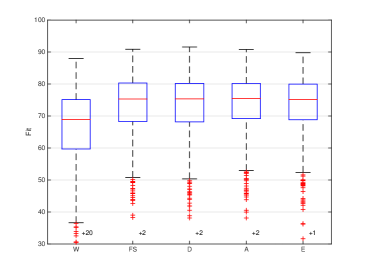
Figure 1: Boxplots of the 1000 fits of the RLS estimates based on the preliminary data-bank and test databank.

6.4 Test Data-Bank

For each test system and each optimal input, we generate a test data record as follows, whose usage is to illustrate the efficacy of the input design. We simulate each test system with the optimal input, treat the unknown inputs according to (29), and get the noise-free output with $N=50$. The noise-free output is then corrupted by an additive white Gaussian noise with the same variance as the additive white Gaussian noise in the preliminary data record. In this way, for each test system and each optimal input, we get 1000 test data records.

6.5 Simulation Results

The simulation results are summarized in Table 6.6 and Fig. 1, where W, FS, D, A, E are used to denote the corresponding simulation results for different inputs, respectively, and W denotes the result corresponding to the white noise input in the preliminary data-bank. In particular, Table 6.6 shows the average model fits and Fig. 1 shows the boxplots of the 1000 model fits, where the model fit (Ljung, 2012) is defined as follows

$$\mbox{\rm Fit}=100\times\left(1-\frac{\|\widehat{\theta}_{N}^{\rm R}-\theta_{0}\|}{\|\theta_{0}-\tilde{\theta}_{0}\|}\right),~{}~{}\tilde{\theta}_{0}=\frac{1}{50}\sum_{k=1}^{50}g_{k}^{0}$$

where $\widehat{\theta}_{N}^{\rm R}$ represents the regularized FIR model estimate (10b) corresponding to each data record, the regression matrix $\Phi$ is constructed by the input according to (29), and the estimated noise variance and TC kernel matrix from the preliminary data record are used.

6.6 Findings

In contrast with the white noise input, all optimal inputs including the one given in Fujimoto & Sugie (2016) and $u^{*}_{\rm D},u^{*}_{\rm A},$ and $u^{*}_{\rm E}$ given in this paper improve the average fit of the regularized FIR model estimate (10b) from 66 to 73 and are more robust. An intuitive explanation for this improvement is that the data records generated by the optimal inputs may have higher average SNRs than the preliminary data record generated by the white noise input. This guess is verified for the data records in this experiment. In addition, the fits of the estimates of the data records generated by all optimal inputs are quite close.

Table 1: Average fits of the regularized FIR model estimate (10b) given in Fig. 1 based on 1000 Monte Carlo runs.

o 0.48 X[1,c]X[1,c]X[1,c]X[1,c]X[1,c]X[1,c] W	FS	D	A	E
66.24	73.56	73.44	73.87	73.46

7 Conclusions

In this paper, the input design of kernel-based regularization method for LTI system identification has been investigated by minimizing the scalar measures of the Bayesian MSE matrix. Under suitable assumption on the unknown inputs and with the introduction of a quadratic map, the non-convex optimization problem associated with the input design problem is transformed into a convex optimization problem. Then based on the global minima of the convex optimization problem, the optimal input is derived by solving the inverse image of the quadratic map. For some special types of fixed kernels, some analytic results provide insights on the input design and also its dependence on the kernel structure.

Appendix A

Appendix A contains the proof of the results in the paper, for which the technical lemmas are placed in Appendix B. The proofs of Propositions 16 and 10 are straightforward and thus omitted.

A.1 Proof of Theorem 7

First, we introduce the cyclic permutation matrix $C\in\mathbb{R}^{N}$ defined by

$$C\displaystyle\stackrel{{\scriptstyle\triangle}}{{=}}\left[\begin{array}[]{cccccc}0&I_{N-1}\\ 1&0\end{array}\right],$$ (108)

which has the following properties

$$C^{i}C^{j}=C^{i+j},C^{N}=I_{N},(C^{i})^{T}=C^{N-i}.$$ (109)

Note that $L_{0}=I_{N}$ and $L_{j}=(C^{j}+(C^{j})^{T})/2$ is real symmetric for $j=1,\dots,n-1$. Clearly, $L_{i}$ commutes with $L_{j}$ by using the properties (109) for $i,j=1,\dots,n-1$ and $i\neq j$. It follows from Theorem B1 in Appendix B that there exists an orthogonal matrix $W$ such that

$$W^{T}L_{j}W=S_{j},~{}j=0,\dots,n-1,$$ (110)

where $S_{j}=\mathrm{diag}[s_{j0},\cdots,s_{j,N-1}]$ is a real diagonal matrix. Therefore, we have

$$f_{j}(u)=u^{T}WS_{j}W^{T}u=\sum_{i=0}^{N-1}s_{ji}z_{i}^{2}$$ (111)

where $z=[z_{0},z_{1},\cdots,z_{N-1}]^{T}=W^{T}u$. We obtain

$$f(u)\!=\!\underbrace{\left[\begin{array}[]{cccc}s_{00}&s_{01}&\cdots&s_{0,N-1}\\ s_{10}&s_{11}&\cdots&s_{1,N-1}\\ \vdots&\vdots&\ddots&\vdots\\ s_{n-1,0}&s_{n-1,1}&\cdots&s_{n-1,N-1}\end{array}\right]}_{S}\!\!\left[\begin{array}[]{c}z_{0}^{2}\\ z_{1}^{2}\\ \vdots\\ z_{N-1}^{2}\\ \end{array}\right].$$ (120)

Since $W^{T}W=I_{N}$, the orthogonal linear mapping $h_{3}(\cdot)$ has the property that the image is $\mathscr{Z}=\{z|z^{T}z=\mathscr{E}\}$. Then the image of $h_{2}(\cdot)$ under $\mathscr{Z}$ is the polytope $\mathscr{X}$ given in (61) by the definition of $h_{2}(\cdot)$. Finally, the conclusion that $\mathscr{F}$ is a polytope follows from that a linear transform of a polytope is still a polytope (Brøndsted, 1983, p. 18, 2.5). This completes the proof.

A.2 Proof of Theorem 8

We only prove the case for even $N$. The proof for odd $N$ is similar and thus omitted.

For convenince, we place the construction of the matrices $W$ and $S$ in Lemma B5. So we first consider the claim $\operatorname*{rank}(S)=\min(N/2+1,n)$, which follows from that the vectors $\xi_{0},\xi_{1},\cdots,\xi_{\frac{N}{2}}$ are orthogonal to each other and $\xi_{j}=\xi_{N-j}$ for $j=0,\dots,N$.

Then note that the polyhedron $\mathscr{X}$ in Theorem 7 can be written as a polytope

$$\mathscr{X}=\mathbf{conv}\left\{d_{0},d_{1},\cdots,d_{N-1}\right\},$$ (121)

where for $j=0,\dots,N-1$, $d_{j}$ is the vector whose elements are zero except the $j\!+\!1$-element that is equal to $\mathscr{E}$. Since $\cos(lj\varpi)=\cos((N-l)j\varpi)$ for any integer $l$ and $j=0,\dots,N\!-\!1$, the matrix $S$ can be expressed in the form of (64).

Now we denote by $\mathscr{C}$ the convex hull of the column vectors of $S$ in (64) and we will show that $\mathscr{F}=\mathscr{C}$. On the one hand, note that

$$Sd_{j}=Sd_{N-j}=\mathscr{E}\xi_{j}(1\!:\!n),~{}j=0,\dots,N/2.$$ (122)

This implies that the image of (121) under the linear transform $h_{1}(x)=Sx$ is included in $\mathscr{C}$ and hence $\mathscr{F}\subset\mathscr{C}$. On the other hand, for each element $r$ in $\mathscr{C}$, there exist $a_{j}\geq 0,j=0,\dots,N/2$ with $\sum_{j=0}^{N/2}a_{j}=1$ such that r=∑_j=0^N/2a_jEξ_j(1​:​n) =S(∑_j=0^N/2a_jd_j)∈F where (122) is used. This concludes $\mathscr{C}\subset\mathscr{F}$. Therefore, we have $\mathscr{F}=\mathscr{C}$. This completes the proof.

A.3 Proof of Proposition 13

First, we show that $r^{\dagger}\in\mathscr{F}$. This can be done by finding a point $x^{0}\in\mathscr{X}$ such that $Sx^{0}=r^{\dagger}$. We can choose $x^{0}=\mathscr{E}[1,\cdots,1]^{T}/N\in\mathscr{X}$. Applying the property that $\xi_{0}$ is orthogonal to the vectors $\{\xi_{j},1\leq j\leq N/2\}$ for even $N$ or $\{\xi_{j},1\leq j\leq(N\!-\!1)/2\}$ for odd $N$ yields $Sx^{0}=r^{\dagger}$. Then we check the gradient of $\log\det(\sigma^{2}Q(r)^{-1})$ with respective to the last $n\!-\!1$ variables of $r$ is zero at $r=r^{\dagger}$. For ridge kernels, we have $\sigma^{2}P^{-1}=\sigma^{2}I_{n}/c$ and accordingly $Q(r^{\dagger})$ is $(\mathscr{E}+\sigma^{2}/c)I_{n}$. Thus we find that

$$-{\rm Tr}(Q(r^{\dagger})^{-1}Q_{i})=0,~{}i=1,\dots,n\!-\!1.$$

Since the problem (51) is strictly convex, $r^{\dagger}$ is the unique stationary point and $r^{*}_{\rm D}=r^{\dagger}$.

The proof for $r^{*}_{\rm A}=r^{\dagger}$ can be derived in a similar way.

A.4 Proof of Theorem 14

The proof of Theorem 14 is the same as that of Proposition 13 since $Q(r^{\dagger})$ is still diagonal in this case.

A.5 Proof of Theorem 15

First, we consider the case $e_{j}>0$ for $j=2,\dots,n$. In this case, we have each element of $Q(r^{\dagger})^{-1}=(\mathscr{E}I_{n}+\sigma^{2}P^{-1})^{-1}$ is positive by Theorem B3. This implies that each element of the gradient at $r=r^{\dagger}$ is negative by (54) and the definition of $Q_{i}$. It follows that [∇logdet(σ^2Q(r^†)^-1)]^T ξ_0(2:n) ¡ 0, since all elements of ${\xi}_{0}(2:n)$ are equal to one. This violates Lemma B6 in Appendix B, which gives the necessary and sufficient condition for $r^{*}_{\rm D}=r^{\dagger}$. Thus $r^{*}_{\rm D}\neq r^{\dagger}$ for this case.

Then we consider the case where $e_{j}<0$ for $j=2,\dots,n$ and $N$ is even. In this case, we have $(Q(r^{\dagger})^{-1})_{ij}>0$ when $|i-j|$ is even and $(Q(r^{\dagger})^{-1})_{ij}<0$ when $|i-j|$ is odd by Theorem B3. This yields that the sign of the $i$-th element $\frac{\partial\log\det(\sigma^{2}Q(r^{\dagger})^{-1})}{\partial r_{i}}$ of the gradient $\nabla\log\det(\sigma^{2}Q(r^{\dagger})^{-1})$ is positive for odd $i$ and negative for even $i$. This shows that [∇logdet(σ^2Q(r^†)^-1)]^T ξ_N/2(2:n) ¡ 0 since the $i$-th element of ${\xi}_{N/2}(2:n)$ is $(-1)^{i}$. This violates the necessary and sufficient condition for $r^{*}_{\rm D}=r^{\dagger}$, and thus $r^{*}_{\rm D}\neq r^{\dagger}$ for this case.

The proof of $r^{*}_{\rm A}\neq r^{\dagger}$ is similar and thus omitted.

A.6 Proof of Corollary 16

The proof is trivial by noting (98) and Theorem 15.

A.7 Proof of Proposition 17

It follows that

$$Q(r^{\dagger})^{-1}\!=\!\frac{1}{\det(Q(r^{\dagger}))}\left[\begin{array}[]{ccccc}\mathscr{E}\!+\!\sigma^{2}p_{2}&\sigma^{2}e\\ \sigma^{2}e&\mathscr{E}\!+\!\sigma^{2}p_{1}\end{array}\right].$$

Then we have $-{\rm Tr}(Q(r^{\dagger})^{-1}Q_{1})=-2\sigma^{2}e/\det(Q(r^{\dagger}))$. In this case, we have ${\xi}_{j}(2:n)={\xi}_{j}(2:2)=\cos(j\varpi)$. As a result, there always exists an index $j$ such that $e$ and $\cos(j\varpi)$ have the same sign for $j=0,\dots,N/2$ when $N$ is even and for $j=0,\dots,(N\!-\!1)/2$ when $N$ is odd. One obtains that $-e\cos(j\varpi)<0$ for this $j$, which violates (139). Therefore, $r^{*}_{\rm D}\neq r^{\dagger}$. The proof of $r^{*}_{\rm A}\neq r^{\dagger}$ is similar and is omitted.

A.8 Proof of Theorem 18

It follows from Lemma B7 in Appendix B that $0$ is an interior point of $\mathscr{F}^{\prime}=\{r^{\prime}\in\mathbb{R}^{n-1}|[\mathscr{E},r^{\prime T}]^{T}\in\mathscr{F}\}$ when $N\geq 2n-2$. Since $P^{-1}$ is nondiagonal, we have $Q(r^{\dagger})^{-1}$ is also nondiagonal. The condition that at least one of the values ${\rm Tr}(Q(r^{\dagger})^{-1}Q_{i})$, $i=1,\dots,n-1$, is nonzero implies that $r^{\dagger}$ is not a stationary point of the problem (51). This means that $r^{*}_{\rm D}\neq r^{\dagger}$. The proof for $r^{*}_{\rm A}\neq r^{\dagger}$ is similar and thus omitted.

A.9 Proof of Corollary 19

For the DC kernel (14), by Theorem B3 as used in the proof of Theorem 15 we have

1. When $\rho>0$, $(Q(r^{\dagger})^{-1})_{ij}>0$ and $(Q(r^{\dagger})^{-2})_{ij}>0$.

2. When $\rho<0$, $(Q(r^{\dagger})^{-1})_{ij}>0$ and $(Q(r^{\dagger})^{-2})_{ij}>0$ if $|i-j|$ is even and $(Q(r^{\dagger})^{-1})_{ij}<0$ and $(Q(r^{\dagger})^{-2})_{ij}<0$ if $|i-j|$ is odd.

This implies that ${\rm Tr}(Q(r^{\dagger})^{-1}Q_{i})\neq 0$ and ${\rm Tr}(Q(r^{\dagger})^{-2}Q_{i})\neq 0$ for all indices $i=1,\dots,n-1$. As a result, the proposition is true by Theorem 18.

Appendix B

This appendix contains the technical lemmas used in the proof in Appendix A.

Theorem B1.

(Jiang & Li, 2016, Theorem 9) Real symmetric matrices $\{I_{N},A_{1},\cdots,A_{m}\}$ with $A_{i}\in\mathbb{R}^{N\times N}$ and $i=1,\dots,m$ are simultaneously diagonalizable via an orthogonal congruent matrix if and only if $A_{i}$ commutes with $A_{j}$ for $i,j=1,2,\cdots,m$ and $i\neq j$.

Theorem B2.

(Gray (2006, Theorem 3.1);Tee (2007)) Denote the circulant matrix $B$ generated by a row vector $b=[b_{0},b_{1},\cdots,b_{N-1}]$ by

$$B={\rm circ}(b)\displaystyle\stackrel{{\scriptstyle\triangle}}{{=}}\left[\begin{array}[]{ccccc}b_{0}&b_{1}&\ddots&b_{N-2}&b_{N-1}\\ b_{N-1}&b_{0}&\ddots&b_{N-3}&b_{N-2}\\ \ddots&\ddots&\ddots&\ddots&\ddots\\ b_{2}&b_{3}&\ddots&b_{0}&b_{1}\\ b_{1}&b_{2}&\ddots&b_{N-1}&b_{0}\end{array}\right].$$ (128)

Then $B$ has unit eigenvectors

$$v^{(m)} =\frac{1}{\sqrt{N}}\big{[}1,\exp(-\iota\varpi m),\cdots,\exp(-\iota\varpi(N\!-\!1)m)\big{]}^{T},$$

$$m =0,\cdots,N\!-1,$$

where $\varpi=2\pi/N$ and $\iota$ is the imaginary unit ($\iota^{2}=-1$), and the corresponding eigenvalues

$$\tau^{(m)} =\sum_{k=0}^{N-1}b_{k}\exp(-\iota mk\varpi)$$

$$=b[1,\exp(-\iota m\varpi),\cdots,\exp(-\iota m(N-1)\varpi)]^{T}$$

and can be expressed by

$$B=A~{}\!\mathrm{diag}([\tau^{(0)},\cdots,\tau^{(N-1)}])A^{H}$$

where $A=[v^{(0)},\cdots,v^{(N-1)}]$ is unitary and $A^{H}$ denotes the complex conjugate transpose of $A$.

Theorem B3.

Let $A$ be a symmetric and positive definite tridiagonal matrix of dimension $n$,

$$A=\left[\begin{array}[]{ccccc}a_{1}&-b_{2}&&&\\ -b_{2}&a_{2}&-b_{3}&&\\ &\ddots&\ddots&\ddots&\\ &&-b_{n-1}&a_{n-1}&-b_{n}\\ &&&-b_{n}&a_{n}\end{array}\right]$$ (134)

and denote the $(i,j)$-element of $A^{-1}$ by $(A^{-1})_{ij}$. Then we have $(A^{-1})_{ij}>0$ when $b_{l}>0$ for $l=2,\dots,n$, while $(A^{-1})_{ij}<0$ if $|i-j|$ is odd and $(A^{-1})_{ij}>0$ if $|i-j|$ is even when $b_{l}<0$ for $l=2,\dots,n$.

Proof B.1.

The result is obtained by applying Theorem 2.3 of Meurant (1992) when $A$ is positive definite.

Theorem B4.

(Boyd & Vandenberghe, 2004, Section 4.2.3, page 139) Let $\varphi:\mathbb{R}^{m}\!\xrightarrow{}\!\mathbb{R}$ be a differentiable convex function, and let $\mathscr{B}\subset\mathbb{R}^{m}$ be a nonempty closed convex set. Consider the problem

$$minimize~{}\varphi(h)~{}~{}subject~{}to~{}h\in\mathscr{B}.$$ (135)

A vector $h^{*}$ is optimal for this problem if and only if $h^{*}\in\mathscr{B}$ and

$$\nabla\varphi(h^{*})^{T}(y-h^{*})\geq 0~{}~{}\mbox{for all}~{}~{}y\in\mathscr{B}$$ (136)

where ∇φ(⋅)=△[∂φ(⋅)∂h1,⋯,∂φ(⋅)∂hm]T is the gradient of $\varphi(\cdot)$ with respect to $h=[h_{1},\cdots,h_{m}]^{T}$.

Lemma B5.

The matrices $\{L_{j},j=0,\cdots,n-1\}$ can be diagonalized simultaneously by the matrix $W$, i.e.,

$$W^{T}L_{j}W=S_{j}=\mathrm{diag}(\xi_{j}),~{}j=0,\dots,n-1.$$ (137)

Proof B.2.

First, we consider the case where $N$ is even. It follows that $L_{0}=I_{N}={\rm circ}([1,0,\cdots,0])$ and $L_{j}={\rm circ}(l_{j}/2),~{}j=1,\cdots,n-1$, where $l_{j}$ is the $N$-dimensional row vector whose elements are zero except that the $j\!+\!1$-th and $N\!-\!j+\!1$-th elements are one. Then by Theorem B2, the eigenvalues of $L_{j}$ are

$$\tau^{(m,j)} =l_{j}[1,\exp(-\iota m\varpi),\cdots,\exp(-\iota m(N-1)\varpi)]^{T}/2$$

$$=\exp(-\iota mj\varpi)/2+\exp(-\iota m(N-j)\varpi)/2$$

$$=\cos(mj\varpi),\ m\!=\!0,\cdots,N\!-\!1,$$

the eigenvectors $\{v^{(m)},m=0,\cdots,N-1\}$ is an orthonormal basis for all matrices $L_{j},j=0,\cdots,n-1$. Moreover, we have $v^{(0)}=\xi_{0}/\sqrt{N}$ and $v^{(N/2)}=\xi_{\frac{N}{2}}/\sqrt{N}$ are real, and $\tau^{(m,j)}\!=\!\tau^{(N-m,j)}$, which implies that the eigenvectors $v^{(m)}$ and $v^{(N-m)}$ of $L_{j}$ correspond to the same eigenvalue $\cos(mj\varpi)$. Thus the linear combinations $(v^{(m)}+{v}^{(N-m)})/2=\xi_{m}/\sqrt{N}$ and $\iota({v}^{(N-m)}-v^{(m)})/2=\zeta_{m}/\sqrt{N}$ of the eigenvectors $v^{(m)}$ and $v^{(N-m)}$ corresponding to the $m$-th and $(N\!-\!m)$-th eigenvalue $\cos(mj\varpi)$ of $L_{j}$ are real and orthogonal. Further we have $|\xi_{m}|=|\zeta_{m}|=\sqrt{N/2}$, and thus {ξ_0,2ξ_1,⋯,2ξ_N-22,ξ_N2,2ζ_N-22,⋯,2ζ_1}/N is a group of real orthonormal eigenvectors of $L_{j}$ and the corresponding eigenvalues are $\{1,\cos(j\varpi),\cdots,\cos((N\!-\!1)j\varpi)\}$, which are actually the elements of $\xi_{j}$. This completes the proof for the case for even $N$. The proof for odd $N$ is similar and thus omitted.

Lemma B6.

The vector $r^{\dagger}\in\mathscr{F}$ is the solution of the problem

$$minimize~{}\varphi(r)~{}~{}subject~{}to~{}r\in\mathscr{F}$$ (138)

where $\varphi(r)$ represents $\log\det(\sigma^{2}Q(r)^{-1})$ or ${\rm Tr}(\sigma^{2}Q(r)^{-1})$, if and only if

$$[\nabla\varphi(r^{\dagger})]^{T}{\xi}_{j}(2:n)\geq 0$$ (139)

with $j=0,\dots,N/2$ for even $N$ or $j=0,\dots,(N\!-\!1)/2$ for odd $N$, where $\nabla\varphi(r^{\dagger})=\left[\frac{\partial\varphi(r^{\dagger})}{\partial r_{1}},\cdots,\frac{\partial\varphi(r^{\dagger})}{\partial r_{n-1}}\right]^{T}$.

Proof B.3.

Note that the first element of each member in $\mathscr{F}$ is $\mathscr{E}$ and hence the first element of the difference $r-r^{\dagger}$ is zero for any $r\in\mathscr{F}$. In addition, we have the last $n-1$ elements of $r^{\dagger}$ are zero. By applying Theorem B4, we see that $r^{\dagger}$ is the solution of (138) if and only if

$$[\nabla\varphi(r^{\dagger})]^{T}(\tilde{r}-0)\geq 0,$$ (140)

where $\tilde{r}$ is any convex linear combination of the points $\{{\xi}_{j}(2:n),j=0,\cdots,N/2\}$ when $N$ is even, namely, $\tilde{r}=\sum_{j=0}^{N/2}a_{j}{\xi}_{j}(2:n)$ with $a_{j}\geq 0$ and $\sum_{j=0}^{N/2}a_{j}=1$. Clearly, the condition (140) is equivalent to (139) for $j=0,\cdots,N/2$. The case when $N$ is odd can be proved in a similar way and thus omitted.

Lemma B7.

The zero vector $0\in\mathbb{R}^{n-1}$ is an interior point of $\mathscr{F}^{\prime}=\{r^{\prime}\in\mathbb{R}^{n-1}|[\mathscr{E},r^{\prime T}]^{T}\in\mathscr{F}\}$ if $N\geq 2n\!-\!2$.

Proof B.4.

This conclusion is proved by considering two cases, respectively: 1) for even $N$ with $N\geq 2n\!-\!2$; 2) for odd $N$ with $N\geq 2n\!-\!1$. Let us explore the first case. It is clear that the dimension of $\mathscr{F}^{\prime}$ is equal to or less than $n-1$. It follows from Theorem 8 that $\operatorname*{rank}(S)=n$. This means that the dimension of $\mathscr{F}^{\prime}$ is $n-1$ and $\mathscr{F}^{\prime}$ consists of all convex combinations of affinely independent $n$ vectors from $\{\mathscr{E}\xi_{j}(2\!:\!n),j=0,\dots,N/2\}$ (Brøndsted, 1983, p. 14, Corollary 2.4). Now we will prove the result by contradiction. Assume that $0$ is not an interior point of $\mathscr{F}^{\prime}$. Thus $0$ must be located on a facet of $\mathscr{F}^{\prime}$ and the dimension of this facet is $n-2$ since the dimension of $\mathscr{F}^{\prime}$ is $n-1$ and hence $0$ is a convex combination of at most $n-1$ affinely independent vectors from $\{\mathscr{E}\xi_{j}(2\!:\!n),j=0,\dots,N/2\}$ (Brøndsted, 1983, Corollary 2.4). In contrast, $0$ can be expressed by a convex combination in the following way

$$0=\frac{1}{N}(\mathscr{E}S(2:n,:))\xi_{0} =\frac{1}{N}\big{(}\mathscr{E}\xi_{0}(2\!:\!n)+\mathscr{E}\xi_{\frac{N}{2}}(2\!:\!n)\big{)}$$

$$~{}~{}~{}~{}+\frac{2}{N}\sum_{j=1}^{\frac{N}{2}-1}(\mathscr{E}\xi_{j}(2\!:\!n))$$ (141)

due to the orthogonal vectors $\{\xi_{j},j=0,1,\cdots\}$ and the expression (64) of $S$. Further, the expression (141) can be rewritten as a convex combination of affinely independent $n$ vectors from $\{\xi_{j}(2\!:\!n),j=0,\dots,N/2\}$ and all the weights are positive since the remaining $N/2+1-n$ vectors of $\{\xi_{j}(2\!:\!n),j=0,\dots,N/2\}$ are convex combinations of these $n$ affinely independent vectors. This contradiction means that the proposition is true. The proof for odd $N$ with $N\geq 2n\!-\!1$ is similar and thus omitted.