Decision-making under uncertainty:
using MLMC for efficient estimation of EVPPI

Abstract

In this paper we develop a very efficient approach to the Monte Carlo estimation of the expected value of partial perfect information (EVPPI) that measures the average benefit of knowing the value of a subset of uncertain parameters involved in a decision model. The calculation of EVPPI is inherently a nested expectation problem, with an outer expectation with respect to one random variable $X$ and an inner conditional expectation with respect to the other random variable $Y$. We tackle this problem by using a Multilevel Monte Carlo (MLMC) method (Giles 2008) in which the number of inner samples for $Y$ increases geometrically with level, so that the accuracy of estimating the inner conditional expectation improves and the cost also increases with level. We construct an antithetic MLMC estimator and provide sufficient assumptions on a decision model under which the antithetic property of the estimator is well exploited, and consequently a root-mean-square accuracy of ${\varepsilon}$ can be achieved at a cost of $O({\varepsilon}^{-2})$. Numerical results confirm the considerable computational savings compared to the standard, nested Monte Carlo method for some simple testcases and a more realistic medical application.

1 Introduction

The motivating applications for this research come from two apparently quite different fields, the funding of medical research and the exploration and exploitation of oil and gas reservoirs. The common element in both cases is decision making under a large degree of uncertainty.

In the medical case (Ades et al. 2004, Brennan et al. 2007) let $X$ and $Y$ represent independent random variables representing the uncertainty in the effectiveness of different medical treatments. In the absence of any knowledge of $X$ or $Y$, then given a finite set of possible treatments $D$, the optimal choice $d_{opt}$ is the one which maximises ${\mathbb{E}}\left[f_{d}(X,Y)\right]$ where $f_{d}(X,Y)$ represents some measure of the patient outcome, such as QALY’s (quality-adjusted life-year), measured on a monetary scale with a larger value being better. Thus, with no knowledge, the optimal outcome on average is

$$\max_{d\in D}\ {\mathbb{E}}\left[f_{d}(X,Y)\right].$$

On the other hand, given perfect information on $X$ and $Y$, through carrying out some new medical research, the best treatment choice maximises $f_{d}(X,Y)$, giving the overall average outcome

$${\mathbb{E}}\left[\,\max_{d\in D}\,f_{d}(X,Y)\right].$$

In the intermediate situation, if $X$ is known but not $Y$, then the best treatment has average outcome value

$${\mathbb{E}}\left[\max_{d}{\mathbb{E}}\left[f_{d}(X,Y)\,|\,X\right]\right].$$

EVPI, the expected value of perfect information, is the difference

$$\mbox{EVPI}={\mathbb{E}}\left[\max_{d}f_{d}(X,Y)\right]-\max_{d}\,{\mathbb{E}}[f_{d}(X,Y)],$$

and EVPPI, the expected value of partial perfect information, is the difference

$$\mbox{EVPPI}={\mathbb{E}}\left[\max_{d}\,{\mathbb{E}}\left[f_{d}(X,Y)\,|\,X\right]\right]-\max_{d}\,{\mathbb{E}}[f_{d}(X,Y)].$$

EVPPI represents the benefit, on average, of knowing the value of $X$. If the value of $X$ represents the information arising from a proposed piece of medical research, then one can compare the cost of the research to the benefits which arise from the information obtained.

In the oil and gas reservoir scenario (Bratvold et al. 2009, Nakayasu et al. 2016), there are also decisions to be made, such as whether or not to drill additional exploratory wells. There is huge uncertainty in various aspects of an oil reservoir, its dimensions, the oil and gas reserves it contains, the rock porosity, etc. An additional well will yield information which will reduce the uncertainty and increase, on average, the amount of oil and gas which will eventually be extracted. However, there is an additional cost in drilling one more well, and the EVPPI will help determine whether or not it is worth it.

The calculation of EVPPI is a nested expectation problem, with an outer expectation over $X$ and an inner conditional expectation over $Y$. In this paper, we choose to focus on the estimation of the difference

$$\mbox{EVPI}-\mbox{EVPPI}={\mathbb{E}}\left[\max_{d}\,f_{d}(X,Y)\right]-{\mathbb{E}}\left[\max_{d}\,{\mathbb{E}}\left[f_{d}(X,Y)\,|\,X\right]\right].$$

EVPI can be estimated directly using standard Monte Carlo methods with independent samples of $(X,Y)$

$$\frac{1}{N}\sum_{n=1}^{N}\max_{d}f_{d}(X^{(n)},Y^{(n)})-\max_{d}\frac{1}{N}\sum_{n=1}^{N}f_{d}(X^{(n)},Y^{(n)}).$$

Assuming each computation $f_{d}(X,Y)$ can be performed with unit cost, EVPI can be estimated with root-mean-square accuracy ${\varepsilon}$ by using $N=O({\varepsilon}^{-2})$ samples $(X^{(n)},Y^{(n)})$ at a total cost which is $O({\varepsilon}^{-2})$. On the other hand, estimating the difference $\mbox{EVPI}-\mbox{EVPPI}$ using standard, nested Monte Carlo methods requires $N$ outer samples of $X$ and $M$ inner samples of $Y$, giving

$$\frac{1}{N}\sum_{n=1}^{N}\left[\frac{1}{M}\sum_{m=1}^{M}\max_{d}f_{d}(X^{(n)},Y^{(n,m)})-\max_{d}\frac{1}{M}\sum_{m=1}^{M}f_{d}(X^{(n)},Y^{(n,m)})\right].$$

As shown in the next section, in order to estimate $\mbox{EVPI}-\mbox{EVPPI}$ with root-mean-square accuracy ${\varepsilon}$ by this estimator, we need $N=O({\varepsilon}^{-2})$ and $M=O({\varepsilon}^{-1/\alpha})$ samples for outer and inner expectations, respectively. Here $\alpha>0$ denotes the order of convergence of the bias and is typically between $1/2$ and $1$. Therefore, the computational complexity will be at least $O({\varepsilon}^{-3})$, and increase up to $O({\varepsilon}^{-4})$ in the worst case.

The aim of this paper is to develop an efficient approach to this nested expectation problem, i.e., the estimation of $\mbox{EVPI}-\mbox{EVPPI}$, by using a Multilevel Monte Carlo (MLMC) method (Giles 2015). MLMC estimators have been used previously for nested expectations of the slightly different form ${\mathbb{E}}[f({\mathbb{E}}[Y|X])]$ by Haji-Ali (2012) and Giles (2015) for cases in which $f$ is twice-differentiable, and by Bujok et al. (2015) for a case in which $f$ is continuous and piecewise linear. Current research (Giles and Haji-Ali 2018) is also looking at the case in which $f$ is a discontinuous indicator (Heaviside) function.

Building on this prior MLMC research, we introduce an antithetic MLMC estimator for $\mbox{EVPI}-\mbox{EVPPI}$ in the next section, and then in Section 3, we provide sufficient assumptions on $f_{d}$’s such that the antithetic property of the estimator is well exploited, and by building upon the basic MLMC theorem (Theorem 1), the estimator is proven to achieve the optimal computational complexity $O({\varepsilon}^{-2})$ (Theorem 3). Numerical experiments in Section 4 confirm the importance of the assumptions made in our theoretical analysis, and also the considerable computational savings compared to the standard, nested Monte Carlo method not only for some simple testcases but also for a more realistic medical application.

2 MLMC method

2.1 Basic MLMC theory

The MLMC method was introduced by Heinrich (2001) for parametric integration, and by Giles (2008) for the estimation of the expectations arising from SDEs. It was subsequently extended to SPDEs (e.g. Cliffe et al. 2011), stochastic reaction networks (Anderson and Higham 2012), and nested simulation (Haji-Ali 2012, Bujok et al. 2015). For an extensive review of MLMC methods, see the review by Giles (2015).

Here we give a brief overview of the MLMC method. The problem we are interested in is to estimate ${\mathbb{E}}[P]$ efficiently for a random output variable $P$ which cannot be sampled exactly. Given a sequence of random variables $P_{0},P_{1},\ldots$ which approximate $P$ with increasing accuracy but also with increasing cost, we have the elementary telescoping summation

$${\mathbb{E}}[P_{L}]={\mathbb{E}}[P_{0}]+\sum_{\ell=1}^{L}{\mathbb{E}}[P_{\ell}-P_{\ell-1}].$$ (1)

The key idea behind the MLMC method is to independently estimate each of the quantities on the r.h.s. of (1) instead of directly estimating the l.h.s., which is the standard Monte Carlo approach. For the same underlying stochastic sample, $P_{\ell}$ and $P_{\ell-1}$ could be well correlated each other, and the variance of the correction $P_{\ell}-P_{\ell-1}$ is expected to get smaller as the level $\ell$ increases. Thus, in order to estimate each of the quantities on the r.h.s. of (1) with the same accuracy, the necessary number of samples for the finest levels becomes much smaller than that for the coarsest levels, resulting in a significant reduction of the total computational cost as compared to the standard Monte Carlo method. This observation leads to the following theorem (Giles 2015):

Theorem 1.

Let $P$ denote a random variable, and let $P_{\ell}$ denote the corresponding level $\ell$ numerical approximation. If there exist independent random variables $Z_{\ell}$ with expected cost $C_{\ell}$ and variance $V_{\ell}$, and positive constants $\alpha,\beta,\gamma,c_{1},c_{2},c_{3}$ such that $\alpha\geq{\textstyle\frac{1}{2}}\min(\beta,\gamma)$ and

• $\displaystyle\left|{\mathbb{E}}[P_{\ell}-P]\right|\leq c_{1}2^{-\alpha\ell}$

• $\displaystyle{\mathbb{E}}[Z_{\ell}]=\left\{\begin{array}[]{ll}{\mathbb{E}}[P_{0}],&\ell=0\\ {\mathbb{E}}[P_{\ell}-P_{\ell-1}],&\ell>0\end{array}\right.$

• $\displaystyle V_{\ell}\leq c_{2}2^{-\beta\ell}$

• $\displaystyle C_{\ell}\leq c_{3}2^{\gamma\ell},$

then there exists a positive constant $c_{4}$ such that for any ${\varepsilon}\!<\!e^{-1}$ there are values $L$ and $N_{\ell}$ for which the multilevel estimator

$$\hat{Z}=\sum_{\ell=0}^{L}\hat{Z}_{\ell}\quad\text{with}\quad\hat{Z}_{\ell}=\frac{1}{N_{\ell}}\sum_{n=1}^{N_{\ell}}Z_{\ell}^{(n)},$$

has a mean-square-error with bound

$$MSE\equiv{\mathbb{E}}\left[\left(\hat{Z}-{\mathbb{E}}[P]\right)^{2}\right]<{\varepsilon}^{2}$$

with a computational complexity $C$ with bound

$${\mathbb{E}}[C]\leq\left\{\begin{array}[]{ll}c_{4}{\varepsilon}^{-2},&\beta>\gamma,\\ c_{4}{\varepsilon}^{-2}(\log{\varepsilon})^{2},&\beta=\gamma,\\ c_{4}{\varepsilon}^{-2-(\gamma-\beta)/\alpha},&\beta<\gamma.\end{array}\right.$$

Remark 1.

In the case where the condition $V_{\ell}\leq c_{2}2^{-\beta\ell}$ can be replaced by ${\mathbb{E}}[Z_{\ell}^{2}]\leq c_{2}2^{-\beta\ell}$, Hölder’s inequality gives

$${\mathbb{E}}[Z_{\ell}]\leq\left({\mathbb{E}}[Z_{\ell}^{2}]\right)^{1/2}\leq\sqrt{c_{2}}2^{-\beta\ell/2}.$$

Using the triangle inequality, we obtain

$$\left|{\mathbb{E}}[P-P_{L}]\right| =\left|\sum_{\ell\geq L}{\mathbb{E}}[P_{\ell+1}-P_{\ell}]\right|=\left|\sum_{\ell\geq L}{\mathbb{E}}[Z_{\ell}]\right|$$

$$\leq\sum_{\ell\geq L}\left|{\mathbb{E}}[Z_{\ell}]\right|\leq\frac{\sqrt{c_{2}}}{1-2^{-\beta/2}}2^{-\beta L/2}.$$

Compared this bound to the condition $\left|{\mathbb{E}}[P_{\ell}-P]\right|\leq c_{1}2^{-\alpha\ell}$, we have $\alpha\geq\beta/2$ and so the assumption $\alpha\geq{\textstyle\frac{1}{2}}\min(\beta,\gamma)$ is simplified into $\alpha\geq\gamma/2$.

As far as possible, we try to develop MLMC estimators which are in the first regime, with $\beta\!>\!\gamma$, so that the total cost is $O({\varepsilon}^{-2})$. This corresponds to $O({\varepsilon}^{-2})$ samples each with an average $O(1)$ cost, and it means that most of the computational cost is incurred on the coarsest levels. When the application is in this regime, Rhee and Glynn (2015) have a technique in which they randomise the selection of the level $\ell$ to obtain a method which is unbiased but has a finite variance and average cost per sample.

Nevertheless, in any regime, Theorem 1 compares favourably with the complexity bound for the standard Monte Carlo method which directly estimates the l.h.s. of (1) based on $N$ Monte Carlo samples of $P_{L}$ for a fixed $L$:

$$\hat{Z}^{\prime}=\frac{1}{N}\sum_{n=1}^{N}P_{L}^{(n)}.$$

In addition to the conditions given in Theorem 1, assume $V:=\sup_{\ell}{\mathbb{V}}[P_{\ell}]<\infty$. For a given accuracy ${\varepsilon}$, let us choose $N=\lceil 2V{\varepsilon}^{-2}\rceil$ and $L=\lceil\log_{2}(\sqrt{2}c_{1}{\varepsilon}^{-1})/\alpha\rceil$, so that the variance and the bias of the estimator are bounded simultaneously:

$${\mathbb{V}}[\hat{Z}^{\prime}]=\frac{{\mathbb{V}}[P_{L}]}{N}\leq\frac{{\mathbb{V}}[P_{L}]}{2V}{\varepsilon}^{2}\leq\frac{{\varepsilon}^{2}}{2},$$

and

$$\left({\mathbb{E}}[P-P_{L}]\right)^{2}\leq\frac{c_{1}^{2}}{2^{2\alpha L}}\leq\frac{{\varepsilon}^{2}}{2},$$

which ensures the mean-square-error bound of $\hat{Z}^{\prime}$

$${\mathbb{E}}\left[(\hat{Z}^{\prime}-{\mathbb{E}}[P])^{2}\right]={\mathbb{V}}[\hat{Z}^{\prime}]+\left({\mathbb{E}}[P-P_{L}]\right)^{2}\leq{\varepsilon}^{2}.$$

Then there exists a positive constant $c_{5}$ such that the expected cost of $\hat{Z}^{\prime}$ is bounded by

$$NC_{L}\leq\left(2V{\varepsilon}^{-2}+1\right)c_{3}2^{\gamma L}\leq\left(2V{\varepsilon}^{-2}+1\right)c_{3}\left(\sqrt{2}c_{1}2^{\alpha}{\varepsilon}^{-1}\right)^{\gamma/\alpha}\leq c_{5}{\varepsilon}^{-2-\gamma/\alpha}.$$

In general, it seems hard to improve the exponent $2+\gamma/\alpha$ of ${\varepsilon}^{-1}$. Therefore, the multilevel estimator always has an asymptotically better complexity bound than the standard Monte Carlo estimator.

2.2 MLMC estimator for EVPPI

In view of the previous subsection, for the estimation of the difference $\mbox{EVPI}-\mbox{EVPPI}$ let us define a random output variable $P$ by

$$P={\mathbb{E}}\left[\max_{d}f_{d}(X,Y)\,|\,X\right]-\max_{d}{\mathbb{E}}\left[f_{d}(X,Y)\,|\,X\right]$$

with the underlying stochastic variable $X$. Obviously $P$ is nothing but the inner conditional expectation of $\mbox{EVPI}-\mbox{EVPPI}$, and the problem we tackle in this paper is rephrased into an efficient estimation of ${\mathbb{E}}[P]$. A sequence of random variables $P_{0},P_{1},\ldots$ is defined by

$$P_{\ell}=\frac{1}{2^{\ell}}\sum_{i=1}^{2^{\ell}}\max_{d}f_{d}(X,Y^{(i)})-\max_{d}\frac{1}{2^{\ell}}\sum_{i=1}^{2^{\ell}}f_{d}(X,Y^{(i)})=:\overline{\max_{d}\,f_{d}}^{\ell}-\max_{d}\,{\overline{f_{d}}}^{\ell}$$

where $\overline{\max_{d}\,f_{d}}^{\ell}$ and ${\overline{f_{d}}}^{\ell}$ represent averages over $2^{\ell}$ independent values of $Y^{(i)}$ for a randomly chosen $X$, respectively. That is to say, $P_{\ell}$ simply denotes the standard Monte Carlo estimator based on $2^{\ell}$ samples for the inner conditional expectation of $\mbox{EVPI}-\mbox{EVPPI}$, so that the sequence $P_{0},P_{1},\ldots$ approximate $P$ with increasing accuracy but also with increasing cost. Namely we have

$$\mbox{EVPI}-\mbox{EVPPI}={\mathbb{E}}[P]=\lim_{\ell\rightarrow\infty}{\mathbb{E}}[P_{\ell}].$$

As discussed above, in order to achieve a given accuracy ${\varepsilon}$, the standard, nested Monte Carlo method chooses $N=O({\varepsilon}^{-2})$ and $M=O(2^{L})=O({\varepsilon}^{-1/\alpha})$, and so the computational complexity is $O({\varepsilon}^{-2-1/\alpha})$. Using the MLMC method, this can be reduced significantly. Following the ideas of Haji-Ali (2012), Bujok et al. (2015), Giles (2015), we use an “antithetic” MLMC estimator

$$\hat{Z}=\sum_{\ell=1}^{L}\hat{Z}_{\ell}\quad\text{with}\quad\hat{Z}_{\ell}=\frac{1}{N_{\ell}}\sum_{n=1}^{N_{\ell}}Z_{\ell}^{(n)},$$

in which

$$Z_{\ell} ={\textstyle\frac{1}{2}}\left(\max_{d}\frac{1}{2^{\ell-1}}\sum_{i=1}^{2^{\ell-1}}f_{d}(X,Y^{(i)})+\max_{d}\frac{1}{2^{\ell-1}}\sum_{i=2^{\ell-1}+1}^{2^{\ell}}f_{d}(X,Y^{(i)})\right)$$

$$\qquad-\max_{d}\frac{1}{2^{\ell}}\sum_{i=1}^{2^{\ell}}f_{d}(X,Y^{(i)})$$

$$=:{\textstyle\frac{1}{2}}\left(\max_{d}{\overline{f_{d}}}^{(a)}+\max_{d}{\overline{f_{d}}}^{(b)}\right)-\max_{d}{\overline{f_{d}}}$$

where, for a randomly chosen $X$,

• ${\overline{f_{d}}}^{(a)}$ is an average of $f_{d}(X,Y)$ over $2^{\ell-1}$ independent samples for $Y$;

• ${\overline{f_{d}}}^{(b)}$ is an average over a second independent set of $2^{\ell-1}$ samples;

• ${\overline{f_{d}}}$ is an average over the combined set of $2^{\ell}$ inner samples.

It is straightforward to see that $\gamma=1$ and ${\mathbb{E}}[Z_{\ell}]={\mathbb{E}}[P_{\ell}\!-\!P_{\ell-1}]$ for $\ell>0$. Here we consider $Z_{0}=P_{0}\equiv 0$, so that the sum of the multilevel estimator over $\ell$ starts from $\ell=1$.

Note that we have the antithetic property ${\textstyle\frac{1}{2}}({\overline{f_{d}}}^{(a)}+{\overline{f_{d}}}^{(b)})-{\overline{f_{d}}}=0$, and therefore $Z_{\ell}\!=\!0$ if the same decision $d$ maximises each of the terms in its definition. This is the key advantage of the antithetic estimator, compared to the alternative ${\overline{f_{d}}}^{(a)}-{\overline{f_{d}}}$.

Remark 2.

It is straightforward to extend the antithetic MLMC approach to estimate EVPI. The difference is that with EVPI all of the underlying random variables $X$ and $Y$ are inner variables; non are outer variables leading to a conditional expectation. Such an MLMC estimator for the maximum of an unconditional expectation has been introduced by Blanchet and Glynn (2015). As discussed in the introduction, however, EVPI can be estimated with $O({\varepsilon}^{2})$ complexity by using standard Monte Carlo methods already, so that the benefit is that one could use a randomisation technique by Rhee and Glynn (2015) to obtain an unbiased estimator, which might be marginal in the current setting.

3 MLMC variance analysis

We first show that the MLMC estimator achieves the nearly optimal complexity of $O({\varepsilon}^{-2}(\log{\varepsilon})^{2})$ under a quite mild assumption.

Theorem 2.

If ${\mathbb{E}}\left[{\mathbb{V}}[f_{d}(X,Y)\,|\,X]\right]$ is finite for all $d$,

$${\mathbb{V}}\left[Z_{\ell}\right]\leq{\mathbb{E}}\left[\left|Z_{\ell}\right|^{2}\right]\leq\frac{6|D|}{2^{\ell}}\sum_{d}{\mathbb{E}}\left[{\mathbb{V}}[f_{d}(X,Y)\,|\,X]\right].$$

Proof.

For any two $|D|$-dimensional vectors with components $a_{d},b_{d}$,

$$\left|\max_{d}a_{d}-\max_{d}b_{d}\right|\leq\max_{d}|a_{d}-b_{d}|\leq\sum_{d}|a_{d}-b_{d}|.$$

Hence, by defining $F_{d}(X)={\mathbb{E}}\left[f_{d}(X,Y)\,|\,X\right]$, we obtain

$$\left|Z_{\ell}\right| =\left|{\textstyle\frac{1}{2}}(\max_{d}{\overline{f_{d}}}^{(a)}+\max_{d}{\overline{f_{d}}}^{(b)})-\max_{d}{\overline{f_{d}}}\right|$$

$$=\left|{\textstyle\frac{1}{2}}(\max_{d}{\overline{f_{d}}}^{(a)}-\max_{d}F_{d})+{\textstyle\frac{1}{2}}(\max_{d}{\overline{f_{d}}}^{(b)}-\max_{d}F_{d})-(\max_{d}{\overline{f_{d}}}-\max_{d}F_{d})\right|$$

$$\leq\sum_{d}\left({\textstyle\frac{1}{2}}|{\overline{f_{d}}}^{(a)}-F_{d}|+{\textstyle\frac{1}{2}}|{\overline{f_{d}}}^{(b)}-F_{d}|+|{\overline{f_{d}}}-F_{d}|\right),$$ (2)

and therefore, by Jensen’s inequality,

$$\left|Z_{\ell}\right|^{2} =\left({\textstyle\frac{1}{2}}(\max_{d}{\overline{f_{d}}}^{(a)}+\max_{d}{\overline{f_{d}}}^{(b)})-\max_{d}{\overline{f_{d}}}\right)^{2}$$

$$\leq|D|\sum_{d}\left({\textstyle\frac{1}{2}}|{\overline{f_{d}}}^{(a)}-F_{d}|+{\textstyle\frac{1}{2}}|{\overline{f_{d}}}^{(b)}-F_{d}|+|{\overline{f_{d}}}-F_{d}|\right)^{2}$$

$$\leq|D|\sum_{d}\left(|{\overline{f_{d}}}^{(a)}\!-\!F_{d}|^{2}+|{\overline{f_{d}}}^{(b)}\!-\!F_{d}|^{2}+2|{\overline{f_{d}}}\!-\!F_{d}|^{2}\right).$$

For the last term in the summand on the right-most side, we have

$${\mathbb{E}}\left[|{\overline{f_{d}}}-F_{d}|^{2}\right]={\mathbb{E}}\left[{\mathbb{E}}\left[|{\overline{f_{d}}}-F_{d}|^{2}\,|\,X\right]\right]=\frac{1}{2^{\ell}}{\mathbb{E}}\left[{\mathbb{V}}\left[f_{d}(X,Y)\,|\,X\right]\right].$$

Similarly

$${\mathbb{E}}\left[|{\overline{f_{d}}}^{(a)}-F_{d}|^{2}\right]={\mathbb{E}}\left[|{\overline{f_{d}}}^{(b)}-F_{d}|^{2}\right]=\frac{1}{2^{\ell-1}}{\mathbb{E}}\left[{\mathbb{V}}\left[f_{d}(X,Y)\,|\,X\right]\right].$$

Hence, ${\mathbb{V}}\left[Z_{\ell}\right]$ is bounded by

$${\mathbb{V}}\left[Z_{\ell}\right] \leq{\mathbb{E}}\left[\left|Z_{\ell}\right|^{2}\right]$$

$$\leq|D|\sum_{d}\left({\mathbb{E}}\left[|{\overline{f_{d}}}^{(a)}-F_{d}|^{2}\right]+{\mathbb{E}}\left[|{\overline{f_{d}}}^{(b)}-F_{d}|^{2}\right]+2{\mathbb{E}}\left[|{\overline{f_{d}}}-F_{d}|^{2}\right]\right).$$

$$=\frac{6|D|}{2^{\ell}}\sum_{d}{\mathbb{E}}\left[{\mathbb{V}}[f_{d}(X,Y)\,|X]\right],$$

which completes the proof. ∎

The theorem shows that the parameters for the MLMC theorem are $\beta=1$, and in view of Remark 1, $\alpha\geq 1/2$. Since $\gamma=1$ by the definition of $Z_{\ell}$, the MLMC estimator is in the second regime, with $\beta=\gamma$, so that the total cost is $O({\varepsilon}^{-2}(\log{\varepsilon})^{2})$. This compares favourably with the cost of $O({\varepsilon}^{-2-1/\alpha})$ for the standard Monte Carlo estimator, where the exponent increases up to $4$ in the worst case. In the proof of the theorem, the antithetic property of the estimator, i.e., ${\textstyle\frac{1}{2}}({\overline{f_{d}}}^{(a)}+{\overline{f_{d}}}^{(b)})-{\overline{f_{d}}}=0$, is not exploited. In fact, the same upper bound on the variance can be obtained even for the alternative ${\overline{f_{d}}}^{(a)}-{\overline{f_{d}}}$. In what follows, we prove a stronger result on the variance under somewhat demanding assumptions to exploit the antithetic structure of $Z_{\ell}$.

In fact, the MLMC variance can be analysed by following the approach used by Giles and Szpruch (2014, Theorem 5.2). Define

$$F_{d}(X)={\mathbb{E}}\left[f_{d}(X,Y)|X\right],~{}~{}~{}~{}d_{opt}(X)=\arg\max_{d}F_{d}(X)$$

so the domain for $X$ is divided into a number of regions in which the optimal decision $d_{opt}(X)$ is unique, with a dividing decision manifold $K$ on which $d_{opt}(X)$ is not uniquely-defined.

Again note that ${\textstyle\frac{1}{2}}({\overline{f_{d}}}^{(a)}+{\overline{f_{d}}}^{(b)})-{\overline{f_{d}}}=0$, and therefore $Z_{\ell}=0$ if the same decision $d$ maximises each of the terms in its definition. When $\ell$ is large and so there are many samples, ${\overline{f_{d}}}^{(a)},{\overline{f_{d}}}^{(b)},{\overline{f_{d}}}$ will all be close to $F_{d}(X)$, and therefore it is highly likely that $Z_{\ell}=0$ unless $X$ is very close to $K$ at which there is more than one optimal decision. This idea leads to an improved theorem on the MLMC variance, but we first need to make three assumptions.

Assumption 1.

${\mathbb{E}}\left[|f_{d}(X,Y)|^{p}\right]$ is finite for all $p\geq 2$.
Comment: this enables us to bound the difference between ${\overline{f_{d}}}^{(a)},{\overline{f_{d}}}^{(b)},{\overline{f_{d}}}$ and $F_{d}(X)$.

Assumption 2.

There exists a constant $c_{0}>0$ such that for all $0<{\epsilon}<1$

$${\mathbb{P}}\left(\min_{x\in K}\|X-x\|\leq{\epsilon}\right)\leq c_{0}{\epsilon}.$$

Comment: this bounds the probability of $X$ being close to the decision manifold $K$.

Assumption 3.

There exist constants $c_{1},c_{2}>0$ such that if $X\notin K$, then

$$\max_{d}F_{d}(X)-\max_{d\neq d_{opt}(X)}F_{d}(X)>\min\left(c_{1},c_{2}\min_{x\in K}\|X-x\|\right).$$

Comment: on $K$ itself there are at least 2 decisions $d_{1},d_{2}$ which yield the same optimal value $F_{d}(X)$; this assumption ensures at least a linear divergence between the values as $X$ moves away from $K$.

Theorem 3.

If Assumptions 1-3 are satisfied, and $Z_{\ell}$ is as defined previously for level $\ell$, then for any $\delta>0$

$${\mathbb{V}}\left[Z_{\ell}\right]=o(2^{-(3/2-\delta)\ell}),\qquad{\mathbb{E}}\left[Z_{\ell}\right]=o(2^{-(1-\delta)\ell}).$$

Comment: a similar $O(N^{-3/2})$ convergence rate for the variance is proved in Theorem 2.3 in (Bujok et al. 2015) for a different nested simulation application.

Before going into the detailed proof of the theorem, we give a heuristic explanation on the variance analysis below:

• Due to Assumption 1 and Lemma 1 shown below, ${\overline{f_{d}}}-F_{d}=O(2^{-\ell/2})$;

• Due to Assumption 2, there is an $O(2^{-\ell/2})$ probability of $X$ being within distance $O(2^{-\ell/2})$ from the decision manifold $K$, in which case $Z_{\ell}=O(2^{-\ell/2})$;

• If $X$ is further away from $K$, Assumption 3 ensures that there is a clear separation between different decision values, and hence the antithetic property of the estimator can be exploited well to give $Z_{\ell}=0$ with high probability;

• This results in

  $${\mathbb{E}}[Z_{\ell}] =O(2^{-\ell/2})\times O(2^{-\ell/2})=O(2^{-\ell}),$$

  $${\mathbb{E}}[Z_{\ell}^{2}] =O(2^{-\ell/2})\times(O(2^{-\ell/2}))^{2}=O(2^{-3\ell/2}),$$

  so that we have $\alpha\approx 1$ and $\beta\approx 3/2$.

To prepare for the proof of the main theorem, we first need a result concerning the deviation of an average of $N$ values from the expected mean. Suppose $X$ is a real random variable with zero mean, and let ${\overline{X}_{\!N}}$ be an average of $N$ i.i.d. samples $X_{n},n=1,2,\ldots,N$. For $p=2$, we have ${\mathbb{E}}[{\overline{X}_{\!N}}^{2}]=N^{-1}{\mathbb{E}}[X^{2}]$, and hence ${\mathbb{P}}[|{\overline{X}_{\!N}}|>c]\leq{\mathbb{E}}[X^{2}]/(c^{2}N)$. For larger values of $p$ for which ${\mathbb{E}}[|X|^{p}]$ is finite, we have the following lemma:

Lemma 1.

For $p\geq 2$, if ${\mathbb{E}}[|X|^{p}]$ is finite then there exists a constant $C_{p}$, depending only on $p$, such that

$${\mathbb{E}}[|{\overline{X}_{\!N}}|^{p}] \leq C_{p}N^{-p/2}{\mathbb{E}}\left[|X|^{p}\right],$$

$${\mathbb{P}}[|{\overline{X}_{\!N}}|>c] \leq C_{p}{\mathbb{E}}[|X|^{p}]/(c^{2}N)^{p/2}.$$

Proof.

The discrete Burkholder-Davis-Gundy inequality (Burkholder et al. 1972) gives us

$${\mathbb{E}}[|{\overline{X}_{\!N}}|^{p}] \leq C_{p}{\mathbb{E}}\left[\left(N^{-2}\sum_{n=1}^{N}X_{n}^{2}\right)^{p/2}\right]$$

$$\leq C_{p}{\mathbb{E}}\left[N^{-p/2-1}\sum_{n=1}^{N}|X_{n}|^{p}\right]=C_{p}N^{-p/2}{\mathbb{E}}\left[|X|^{p}\right],$$

where $C_{p}$ is a constant depending only on $p$. The second result follows immediately from the Markov inequality. ∎

Proof of Theorem 3.

The analysis follows the approach used by Giles et al. (2009) and Giles and Szpruch (2014, Theorem 5.2).

For a particular value of $\delta$, we define ${\epsilon}=2^{-(1/2-\delta/2)\ell}$, and consider the events

$$A \equiv\left\{\min_{x\in K}\|X-x\|\leq{\epsilon}\right\},$$

$$B \equiv\displaystyle\bigcup_{d}\left\{\max\left(|{\overline{f_{d}}}^{(a)}-F_{d}|,|{\overline{f_{d}}}^{(b)}-F_{d}|,|{\overline{f_{d}}}-F_{d}|\right)\geq{\textstyle\frac{1}{2}}c_{2}{\epsilon}\right\},$$

where $c_{2}$ is as defined in Assumption 3.

Using ${\bf{1}}_{A}$ to indicate the indicator function for event $A$, and $A^{c}$ to denote the complement of $A$, we have

$${\mathbb{E}}\left[\left({\textstyle\frac{1}{2}}(\max_{d}{\overline{f_{d}}}^{(a)}+\max_{d}{\overline{f_{d}}}^{(b)})-\max_{d}{\overline{f_{d}}}\right)^{2}\right]$$

$$={\mathbb{E}}\left[\left({\textstyle\frac{1}{2}}(\max_{d}{\overline{f_{d}}}^{(a)}+\max_{d}{\overline{f_{d}}}^{(b)})-\max_{d}{\overline{f_{d}}}\right)^{2}{\bf{1}}_{A\cup B}\right]$$

$$\quad+{\mathbb{E}}\left[\left({\textstyle\frac{1}{2}}(\max_{d}{\overline{f_{d}}}^{(a)}+\max_{d}{\overline{f_{d}}}^{(b)})-\max_{d}{\overline{f_{d}}}\right)^{2}{\bf{1}}_{A^{c}\cap B^{c}}\right].$$ (3)

Looking at the first of the two terms on the r.h.s. of (3), then Hölder’s inequality gives

$${\mathbb{E}}\left[\left({\textstyle\frac{1}{2}}(\max_{d}{\overline{f_{d}}}^{(a)}+\max_{d}{\overline{f_{d}}}^{(b)})-\max_{d}{\overline{f_{d}}}\right)^{2}{\bf{1}}_{A\cup B}\right]$$

$$\leq{\mathbb{E}}\left[\left({\textstyle\frac{1}{2}}(\max_{d}{\overline{f_{d}}}^{(a)}+\max_{d}{\overline{f_{d}}}^{(b)})-\max_{d}{\overline{f_{d}}}\right)^{2p}\right]^{1/p}\left({\mathbb{P}}(A)+{\mathbb{P}}(B)\right)^{1/q}$$

for any $p,q\geq 1$, with $p^{-1}+q^{-1}=1$.

Now, ${\mathbb{P}}(A)\leq c_{0}\,{\epsilon}$ due to Assumption 1, and

$${\mathbb{P}}(B)\leq\sum_{d}\left({\mathbb{P}}(|{\overline{f_{d}}}^{(a)}-F_{d}|\geq{\textstyle\frac{1}{2}}{\epsilon})+{\mathbb{P}}(|{\overline{f_{d}}}^{(b)}-F_{d}|\geq{\textstyle\frac{1}{2}}{\epsilon})+{\mathbb{P}}(|{\overline{f_{d}}}-F_{d}|\geq{\textstyle\frac{1}{2}}{\epsilon})\right).$$

Due to Lemma 1,

$${\mathbb{P}}(\,|{\overline{f_{d}}}-F_{d}|\geq{\textstyle\frac{1}{2}}{\epsilon}\,|\,X)={\mathbb{E}}\left[{\bf 1}_{|{\overline{f_{d}}}-F_{d}|\geq{\textstyle\frac{1}{2}}{\epsilon}}\,|\,X\right]\leq C_{m}{\mathbb{E}}\left[|f_{d}-F_{d}|^{m}\,|\,X\right]/({\epsilon}^{2}2^{\ell})^{m/2},$$

for any $m\geq 2$. Taking an outer expectation with respect to $X$, the tower property then gives

$${\mathbb{P}}(|{\overline{f_{d}}}-F_{d}|\geq{\textstyle\frac{1}{2}}{\epsilon})={\mathbb{E}}\left[{\bf 1}_{|{\overline{f_{d}}}-F_{d}|\geq{\textstyle\frac{1}{2}}{\epsilon}}\right]\leq C_{m}{\mathbb{E}}\left[|f_{d}-F_{d}|^{m}\right]/({\epsilon}^{2}2^{\ell})^{m/2}.$$

Similar bounds exists for ${\mathbb{P}}(|{\overline{f_{d}}}^{(a)}-F_{d}|\geq{\textstyle\frac{1}{2}}{\epsilon})$ and ${\mathbb{P}}(|{\overline{f_{d}}}^{(b)}-F_{d}|\geq{\textstyle\frac{1}{2}}{\epsilon})$. We can take $m$ to be sufficiently large so that ${\textstyle\frac{1}{2}}m-{\textstyle\frac{1-\delta}{2}}m>{\textstyle\frac{1-\delta}{2}}$ and hence ${\mathbb{P}}(B)=o(2^{-(1-\delta)\ell/2})$. Then, $q$ can be chosen sufficiently close to 1 so that $\left({\mathbb{P}}(A)+{\mathbb{P}}(B)\right)^{1/q}\ =\ o(2^{-(1/2-\delta)\ell}).$

Applying Jensen’s inequality to (2) twice, we obtain

$$\left({\textstyle\frac{1}{2}}(\max_{d}{\overline{f_{d}}}^{(a)}+\max_{d}{\overline{f_{d}}}^{(b)})-\max_{d}{\overline{f_{d}}}\right)^{2p}$$

$$\leq|D|^{2p-1}\sum_{d}\left({\textstyle\frac{1}{2}}|{\overline{f_{d}}}^{(a)}-F_{d}|+{\textstyle\frac{1}{2}}|{\overline{f_{d}}}^{(b)}-F_{d}|+|{\overline{f_{d}}}-F_{d}|\right)^{2p}$$

$$\leq(2|D|)^{2p-1}\sum_{d}\left({\textstyle\frac{1}{2}}|{\overline{f_{d}}}^{(a)}-F_{d}|^{2p}+{\textstyle\frac{1}{2}}|{\overline{f_{d}}}^{(b)}-F_{d}|^{2p}+|{\overline{f_{d}}}-F_{d}|^{2p}\right).$$

It follows from Lemma 1 that

$${\mathbb{E}}[\,|{\overline{f_{d}}}-F_{d}|^{2p}] ={\mathbb{E}}\left[{\mathbb{E}}[|{\overline{f_{d}}}-F_{d}|^{2p}\,|\,X]\right]$$

$$\leq C_{2p}2^{-p\ell}{\mathbb{E}}\left[{\mathbb{E}}[|f_{d}(X,Y)-{\mathbb{E}}[f_{d}(X,Y)\,|\,X]|^{2p}\,|\,X]\right]$$

$$=C_{2p}2^{-p\ell}{\mathbb{E}}[|f_{d}(X,Y)-{\mathbb{E}}[f_{d}(X,Y)]|^{2p}],$$

so Assumption 1 implies that ${\mathbb{E}}[|{\overline{f_{d}}}-F_{d}|^{2p}]=O(2^{-p\ell})$, with similar bounds for ${\overline{f_{d}}}^{(a)}$ and ${\overline{f_{d}}}^{(b)}$. Hence,

$${\mathbb{E}}\left[\left({\textstyle\frac{1}{2}}(\max_{d}{\overline{f_{d}}}^{(a)}+\max_{d}{\overline{f_{d}}}^{(b)})-\max_{d}{\overline{f_{d}}}\right)^{2p}\right]^{1/p}=O(2^{-\ell}),$$

and therefore the first term on the r.h.s. of (3) has bound $o(2^{-(3/2-\delta)\ell})$.

We now consider the second term on the r.h.s. of (3). For any sample in $A^{c}\cap B^{c}$, we have $\displaystyle\min_{x\in K}\|X-x\|\geq{\epsilon},$ and $|{\overline{f_{d}}}^{(a)}-F_{d}|<{\textstyle\frac{1}{2}}c_{2}{\epsilon},~{}|{\overline{f_{d}}}^{(b)}-F_{d}|<{\textstyle\frac{1}{2}}c_{2}{\epsilon},~{}|{\overline{f_{d}}}-F_{d}|<{\textstyle\frac{1}{2}}c_{2}{\epsilon},$ for all $d$. For a particular outer sample $X$, if $d\neq d_{opt}(X)$ then using Assumption 3 we have

$${\overline{f_{d}}}_{opt}-{\overline{f_{d}}} =({F_{d}}_{opt}-F_{d})+({\overline{f_{d}}}_{opt}-{F_{d}}_{opt})-({\overline{f_{d}}}-F_{d})$$

$$>\min(c_{1},c_{2}{\epsilon})-{\textstyle\frac{1}{2}}c_{2}{\epsilon}-{\textstyle\frac{1}{2}}c_{2}{\epsilon}=\min(c_{1}-c_{2}{\epsilon},0)$$

If $\ell$ is sufficiently large so that $c_{2}{\epsilon}<c_{1}$, then ${\overline{f_{d}}}_{opt}-{\overline{f_{d}}}>0$ and hence $d_{opt}=\arg\max_{d}{\overline{f_{d}}}$. The same argument applies to ${\overline{f_{d}}}_{opt}^{(a)}-{\overline{f_{d}}}^{(a)}$ and ${\overline{f_{d}}}_{opt}^{(b)}-{\overline{f_{d}}}^{(b)}$, so the conclusion is that in all three cases, $d_{opt}$ is the decision which maximises ${\overline{f_{d}}}^{(a)}$, ${\overline{f_{d}}}^{(b)}$ and ${\overline{f_{d}}}$, and therefore

$${\textstyle\frac{1}{2}}(\max_{d}{\overline{f_{d}}}^{(a)}+\max_{d}{\overline{f_{d}}}^{(b)})-\max_{d}{\overline{f_{d}}}={\textstyle\frac{1}{2}}({\overline{f_{d}}}_{opt}^{(a)}+{\overline{f_{d}}}_{opt}^{(b)})-{\overline{f_{d}}}_{opt}=0.$$

Hence, for sufficiently large $\ell$, the second term is zero, which concludes the proof for the bound on ${\mathbb{V}}[Z_{\ell}]$ and the bound on ${\mathbb{E}}[Z_{\ell}]$ is obtained similarly. ∎

The conclusion from the theorem is that the parameters for the MLMC theorem are $\beta\!\approx\!3/2$, $\alpha\!\approx\!1$, and $\gamma\!=\!1$, giving the optimal complexity of $O({\varepsilon}^{-2})$. Again, this compares favourably with the cost of $O({\varepsilon}^{-3})$ for the standard Monte Carlo estimator.

4 Numerical results

4.1 Simple test cases

To validate the importance of the assumptions made in the variance analysis, several simple examples are tested here. Let $X$ and $Y$ be independent univariate standard normal random variables, and let us consider two-treatment decision problems with $f_{1}(X,Y)=0$ and either

1. $f_{2}(X,Y)=X+Y$,

2. $f_{2}(X,Y)=X^{3}+Y$, or

3. $f_{2}(X,Y)=\begin{cases}X+Y+1,&X<-1,\\ Y,&-1\leq X\leq 1,\\ X+Y-1,&X>1.\end{cases}$

It is easy to check that this simple test case with the first choice of $f_{2}$ satisfies all of Assumptions 1-3, while the other cases with the second and third choices of $f_{2}$ do not. With the second choice of $f_{2}$, we have $F_{1}(X)=0$ and $F_{2}(X)=X^{3}$, so that $K=\{0\}\subset{\mathbb{R}}$ and

$$\max_{d}F_{d}(X)-\max_{d\neq d_{opt}(X)}F_{d}(X)\ =\ |X|^{3},$$

which implies that there exist no constants $c_{1},c_{2}>0$ such that Assumption 3 is satisfied. For the third choice of $f_{2}$, we have $K=[-1,1]\subset{\mathbb{R}}$ whose probability measure is not zero. Hence, by considering the limiting situation ${\epsilon}\to 0$ in Assumption 2, we see that there exists no constant $c_{0}>0$ such that Assumption 2 is satisfied.

The results for the first choice of $f_{2}$ are shown in Figure 1. The left top plot shows the behaviours of the variances of both $P_{\ell}$ and $Z_{\ell}$, where the variances are estimated by using $N=2\times 10^{5}$ random samples at each level. Note that the logarithm of the empirical variance in base $2$ versus the level is plotted here. The slope of the line for $Z_{\ell}$ is $-1.43$, indicating that ${\mathbb{V}}[Z_{\ell}]=O(2^{-1.43\ell})$. This result is in good agreement with Theorem 3 which holds for decision models satisfying Assumptions 1-3.

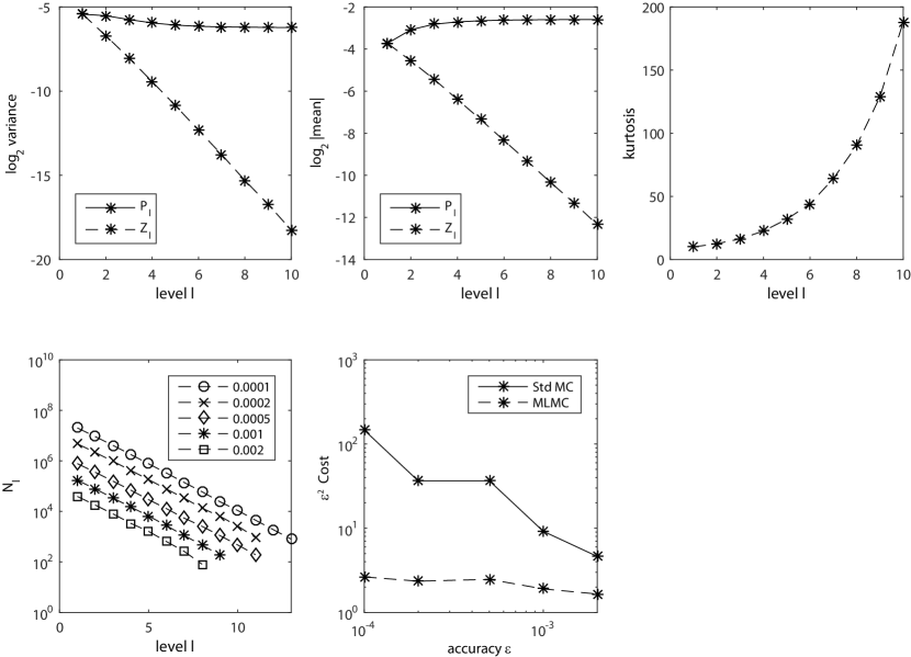
Figure 1: MLMC results for simple test case with the first choice of $f_{2}$.

The middle top plot shows the behaviours of the estimated mean values of both $P_{\ell}$ and $Z_{\ell}$. The slope of the line for $Z_{\ell}$ is approximately $-1$, which implies that ${\mathbb{E}}[Z_{\ell}]=O(2^{-\ell})$. This is again in good agreement with Theorem 3.

The right top plot shows the behaviour of the estimated kurtosis of $Z_{\ell}$. The way in which the kurtosis increases with the level also confirms that the MLMC corrections are increasingly dominated by a few rare samples yielding $Z_{\ell}\neq 0$, corresponding to outer samples $X$ which are close to the decision manifold $K$ across which the optimal decision $d_{opt}$ changes.

Using the implementation due to Giles (2015, Algorithm 1), the maximum level $L$ and the computational costs $N_{\ell}$ for levels $\ell=1,\ldots,L$, required for the combined multilevel estimator to achieve an MSE less than ${\varepsilon}^{2}$, are estimated. Each line in the left bottom plot shows the values of $N_{\ell}$, $\ell=1,\ldots,L$, for a particular value of ${\varepsilon}$. As expected, the number of samples varies with the level such that many more samples are allocated on the coarsest levels, which is in good agreement with the optimal allocation of computational effort given by $N_{\ell}\propto{\varepsilon}^{-2}\sqrt{V_{\ell}/C_{\ell}}\propto{\varepsilon}^{-2}2^{-(\beta+\gamma)\ell/2}$ (Giles 2015). It is also shown here that, as the value of ${\varepsilon}$ decreases, the maximum level $L$ increases to ensure the weak convergence $|{\mathbb{E}}\left[P-P_{L}\right]|\leq{\varepsilon}/\sqrt{2}$.

The middle bottom plot shows the behaviour of the total computational cost

$$C=\sum_{\ell=1}^{L}2^{\ell}N_{\ell},$$

to achieve an MSE less than ${\varepsilon}^{2}$. Since it is expected from the MLMC theorem that ${\varepsilon}^{2}C$ is independent of ${\varepsilon}$, we plot ${\varepsilon}^{2}C$ versus ${\varepsilon}$ here. Indeed, it can be seen that ${\varepsilon}^{2}C$ is only slightly dependent on ${\varepsilon}$, indicating that the MLMC estimator gives the optimal complexity of $O({\varepsilon}^{-2})$. This result compares favourably with the result for the standard (in this case, nested) Monte Carlo method. The superiority of the MLMC method becomes more evident as the desired accuracy ${\varepsilon}$ decreases. For instance, for ${\varepsilon}=10^{-4}$, the MLMC method is more than 50 times more efficient.

Let us move on to the second and third choices of $f_{2}$. Since these test cases do not satisfy one of Assumptions 1-3, Theorem 3 does not apply and it is expected from Theorem 2 that the MLMC estimator achieves the nearly optimal complexity of $O({\varepsilon}^{-2}(\log{\varepsilon})^{2})$. The results for the second and third choices of $f_{2}$ are shown in Figures 2 and 3, respectively.

For the second choice of $f_{2}$, it is seen from the first two top plots that the slopes of the lines for the variance and the mean value of $Z_{\ell}$ are $-1.12$ and $-0.64$, respectively, which are slightly better than the values $-1$ and $-0.5$ which are to be expected from the theory. In the right top plot, the kurtosis increases with the level but not so significantly as compared to the first test case. Because of a smaller value of $\alpha$, we can observe in the left bottom plot that the maximum level to ensure the weak convergence becomes large. Still, the superiority of the MLMC method over the standard Monte Carlo method is prominent. For ${\varepsilon}=10^{-4}$, the MLMC method is approximately 3000 times more efficient. Similar results are also obtained for the third choice of $f_{2}$.

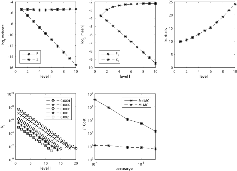
Figure 2: MLMC results for simple test case with the second choice of $f_{2}$.

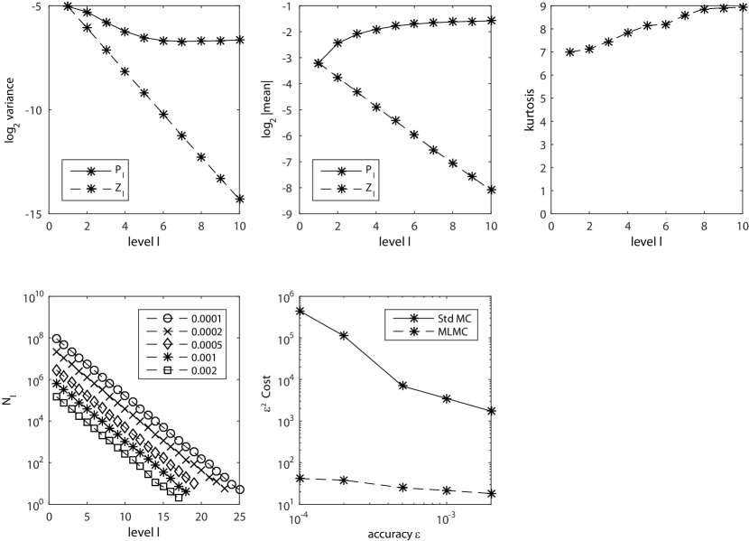
Figure 3: MLMC results for simple test case with the third choice of $f_{2}$.

4.2 Medical decision model

To demonstrate the practical usefulness of the MLMC estimator, the medical decision model introduced in Brennan et al. (2007) is tested. Let $X\cup Y=(X_{1},\ldots,X_{19})$ with each univariate random variable $X_{j}$ following the normal distribution with mean $\mu_{j}$ and standard deviation $\sigma_{j}$ independently except that $X_{5},X_{7},X_{14},X_{16}$ are pairwise correlated with a correlation coefficient $\rho=0.6$. The values for $\mu_{j}$ and $\sigma_{j}$ and the medical meaning of $X_{j}$ are listed in Table 1. The problem to be tested is a two-treatment decision problem with

$$f_{1}(X,Y) = \lambda\left(X_{5}X_{6}X_{7}+X_{8}X_{9}X_{10}\right)-(X_{1}+X_{2}X_{3}X_{4}),\ \text{and}$$

$$f_{2}(X,Y) = \lambda\left(X_{14}X_{15}X_{16}+X_{17}X_{18}X_{19}\right)-(X_{11}+X_{12}X_{13}X_{4}),$$

where $\lambda$ denotes the monetary valuation of health and is set to $10^{4}$ ($\pounds$). In what follows, we call this decision model the BKOC test case, named after the authors of Brennan et al. (2007).

Table 1: Variables in the BKOC test case (Table 2 in Brennan et al. (2007)).

variable	$\mu_{j}$	$\sigma_{j}$	meaning
$X_{1}$	1000	1	Cost of drug ($\pounds$)
$X_{2}$	0.1	0.02	Probability of admissions
$X_{3}$	5.2	1.0	Days in hospital
$X_{4}$	400	200	Cost per day ($\pounds$)
$X_{5}$	0.7	0.1	Probability of responding
$X_{6}$	0.3	0.1	Utility change if response
$X_{7}$	3.0	0.5	Duration of response (years)
$X_{8}$	0.25	0.1	Probability of side effects
$X_{9}$	-0.1	0.02	Change in utility if side effect
$X_{10}$	0.5	0.2	Duration of side effect (years)
$X_{11}$	1500	1	Cost of drug ($\pounds$)
$X_{12}$	0.08	0.02	Probability of admissions
$X_{13}$	6.1	1.0	Days in hospital
$X_{14}$	0.8	0.1	Probability of responding
$X_{15}$	0.3	0.05	Utility change if response
$X_{16}$	3.0	1.0	Duration of response (years)
$X_{17}$	0.2	0.05	Probability of side effects
$X_{18}$	-0.1	0.02	Change in utility if side effect
$X_{19}$	0.5	0.2	Duration of side effect (years)

The results for the BKOC test case with $X=(X_{5},X_{14})$ are shown in Figure 4. From the first two top plots we see that the slopes of the lines for the variance and the mean value of $Z_{\ell}$ are $-1.352$ and $-0.89$, respectively, indicating that the MLMC estimator is in the first regime, with $\beta>\gamma$. The behaviour of the kurtosis of $Z_{\ell}$, shown in the right top plot, is quite similar to that observed for the simple test case with the first choice of $f_{2}$. As expected, most of the computational cost is actually incurred on the coarsest levels, and the MLMC method gives savings of factor more than 100 as compared to the standard Monte Carlo method for the desired accuracy ${\varepsilon}=0.1$.

As shown in Figure 5 and 6, respectively, both of the results for the BKOC test case with $X=(X_{5},X_{6},X_{14},X_{15})$ and $X=(X_{7},X_{16})$ are quite similar to the case with $X=(X_{5},X_{14})$, and the MLMC method gives savings of factor up to 100.

In order to achieve an MSE less than 1, the MLMC method needs the total computational costs of $C=4.1\times 10^{7},3.0\times 10^{7},2.2\times 10^{7}$ for the three respective cases, giving the estimates of the difference $\mbox{EVPI}-\mbox{EVPPI}$ as 799, 206, and 509. The total computational costs for the standard Monte Carlo method are found to be approximately 10 times larger for all cases. The standard Monte Carlo method using $10^{7}$ random samples of $(X,Y)$ yields the estimate of EVPI as 1047. Thus, the EVPPI values for the three cases are estimated as 248, 841 and 538.

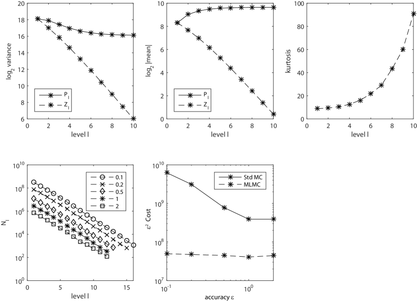
Figure 4: MLMC results for the BKOC test case with $X=(X_{5},X_{14})$.

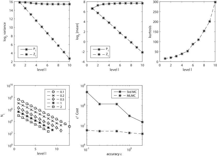
Figure 5: MLMC results for the BKOC test case with $X=(X_{5},X_{6},X_{14},X_{15})$.

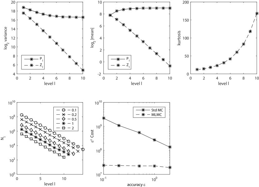
Figure 6: MLMC results for the BKOC test case with $X=(X_{7},X_{16})$.

5 Conclusions

In this paper we have developed a Multilevel Monte Carlo method for the estimation of the expected value of partial perfect information, EVPPI, which is one of the most demanding nested expectation applications. The essential difficulty in the theoretical analysis lies in how to deal with the maximum of an unconditional expectation. We provide a set of assumptions on a decision model to exploit the antithetic property of the estimator, and then numerical analysis proves that a root-mean-square accuracy of ${\varepsilon}$ can be achieved at a computational cost which is $O({\varepsilon}^{-2})$, and this is also supported by numerical experiments. As we already announced in (Giles et al. 2017), the MLMC estimator introduced in this paper works quite well for real medical application which measures the cost-effectiveness of novel oral anticoagulants in atrial fibrillation. The details on this application shall be summarised in the near future.

Future research will address the following topics:

• an extension to handle input distributions which are defined empirically, such as through the use of MCMC methods to sample from a Bayesian posterior distribution;

• the use of quasi-random numbers in place of pseudo-random numbers, which leads to the Multilevel Quasi-Monte Carlo method which is capable of additional substantial savings (Giles and Waterhouse 2009);

• the use of an adaptive number of inner samples, following the ideas of Broadie et al. (2011), since it is only the outer samples which are near the decision manifold $K$ which require great accuracy for the inner conditional expectation.

References

- Ades et al. (2004) Ades AE, Lu G, Claxton K (2004) Expected value of sample information calculations in medical decision modeling. Medical Decision Making 24:207–227.
- Anderson and Higham (2012) Anderson D, Higham D (2012) Multi-level Monte Carlo for continuous time Markov chains, with applications in biochemical kinetics. SIAM Multiscale Modelling and Simulation 10(1):146–179.
- Blanchet and Glynn (2015) Blanchet J, Glynn P (2015) Unbiased Monte Carlo for optimization and functions of expectations via multi-level randomization. Proceedings of the 2015 Winter Simulation Conference, 3656–3667, IEEE.
- Bratvold et al. (2009) Bratvold R, Bickel J, Lohne H (2009) Value of information in the oil and gas industry: past, present, and future. SPE Reservoir Evaluation and Engineering 12:630–638.
- Brennan et al. (2007) Brennan A, Kharroubi S, O’Hagan A, Chilcott J (2007) Calculating partial expected value of perfect information via Monte Carlo sampling algorithms. Medical Decision Making 27:448–470.
- Broadie et al. (2011) Broadie M, Du Y, Moallemi C (2011) Efficient risk estimation via nested sequential simulation. Management Science 57(6):1172–1194.
- Bujok et al. (2015) Bujok K, Hambly B, Reisinger C (2015) Multilevel simulation of functionals of Bernoulli random variables with application to basket credit derivatives. Methodology and Computing in Applied Probability 17(3):579–604.
- Burkholder et al. (1972) Burkholder D, Davis B, Gundy R (1972) Integral inequalities for convex functions of operators on martingales. Proc. Sixth Berkeley Symposium Math. Statist. Prob., Vol II, 223–240 (University of California Press, Berkeley).
- Cliffe et al. (2011) Cliffe K, Giles M, Scheichl R, Teckentrup A (2011) Multilevel Monte Carlo methods and applications to elliptic PDEs with random coefficients. Computing and Visualization in Science 14(1):3–15.
- Giles (2008) Giles M (2008) Multilevel Monte Carlo path simulation. Operations Research 56(3):607–617.
- Giles (2015) Giles M (2015) Multilevel Monte Carlo methods. Acta Numerica 24:259–328.
- Giles et al. (2017) Giles M, Goda T, Thom H, Fang W, Wang Z (2017) MLMC for estimation of expected value of partial perfect information. Presentation at International Conference on Monte Carlo Methods and Applications.
- Giles et al. (2009) Giles M, Higham D, Mao X (2009) Analysing multilevel Monte Carlo for options with non-globally Lipschitz payoff. Finance and Stochastics 13(3):403–413.
- Giles and Haji-Ali (2018) Giles M, Haji-Ali AL (2018) Multilevel nested simulation for efficient risk estimation. arXiv pre-print 1802.05016.
- Giles and Szpruch (2014) Giles M, Szpruch L (2014) Antithetic multilevel Monte Carlo estimation for multi-dimensional SDEs without Lévy area simulation. Annals of Applied Probability 24(4):1585–1620.
- Giles and Waterhouse (2009) Giles M, Waterhouse B (2009) Multilevel quasi-Monte Carlo path simulation. Advanced Financial Modelling, 165–181, Radon Series on Computational and Applied Mathematics (De Gruyter).
- Haji-Ali (2012) Haji-Ali AL (2012) Pedestrian flow in the mean-field limit. MSc thesis, KAUST, URL http://stochastic_numerics.kaust.edu.sa/Documents/publications/AbdulLateef%20Haji%20Ali%20_Thesis.pdf.
- Heinrich (2001) Heinrich S (2001) Multilevel Monte Carlo methods. Multigrid Methods, volume 2179 of Lecture Notes in Computer Science, 58–67 (Springer).
- Nakayasu et al. (2016) Nakayasu M, Goda T, Tanaka K, Sato K (2016) Evaluating the value of single-point data in heterogeneous reservoirs with the expectation maximization. SPE Economics and Management 8:1–10.
- Rhee and Glynn (2015) Rhee CH, Glynn P (2015) Unbiased estimation with square root convergence for SDE models. Operations Research 63(5):1026–1043.