Numerical Algorithm for Optimal Control of Continuity Equations

Abstract

An optimal control problem for the continuity equation is considered. The aim of a controller is to maximize the total mass within a target set at a given type moment. An iterative numerical algorithm for solving this problem is presented.

2010 Mathematics Subject Classification: 49M05

Keywords: continuity equation, Liouville equation, optimal control, numerical method.

1 Introduction

Consider a mass distributed on $\mathbb{R}^{n}$ that drifts along a controlled vector field $\mathbf{v}=\mathbf{v}(t,x,u)$. The aim of the controller is to bring as much mass as possible to a target set $A$ by a time moment $T$.

Let us give the precise mathematical statement of the problem. Suppose that $\rho=\rho(t,x)$ is the density of the distribution and $u=u(t)$ is a strategy of the controller. Then, $\rho$ evolves in time according to the continuity equation

$$\begin{cases}\rho_{t}+\mathop{\rm div}{}_{x}\left(\mathbf{v}\left(t,x,u(t)\right)\rho\right)=0,\\ \rho(0,x)=\rho_{0}(x),\end{cases}$$ (1.1)

where $\rho_{0}$ denotes the initial density. Our aim is to find a control $u$ that maximizes the following integral

$$J[u]=\int_{A}\rho(T,x)\mathinner{\mathrm{d}{x}}.$$ (1.2)

Typically, $u$ belongs to a set $\mathcal{U}$ of admissible controls. Here we take the following one:

$$\mathcal{U}=\left\{u(\cdot)\;\text{is measurable},\;u(t)\in U\;\text{ a.e. }\;t\in[0,T]\right\},$$ (1.3)

where $U$ is a compact subset of $\mathbb{R}^{m}$.

In this paper we propose an iterative method for solving problem (1.1)–(1.3), which is based on the needle linearization algorithm for classical optimal control problems [3]. Given an initial guess $u^{0}$, the algorithm produces a sequence of controls $u^{k}$ with the property $J[u^{k+1}]\geq J[u^{k}]$, for all $k\in\mathbb{N}$.

A different approach for numerical solution of (1.1)–(1.3) was proposed by S. Roy and A. Borzì in [2]. The authors used a specific discretization of (1.1) to produce a finite dimensional optimization problem. It seems difficult to compare the efficiency of both algorithms, because one was tested for 2D and the other for 1D problems.

Finally, let us remark that problem (1.1)–(1.3) is equivalent to the following optimal control problem for an ensemble of dynamical systems:

$$\text{Maximize}\quad\int\rho_{0}(x)\mathinner{\mathrm{d}{x}}\quad\text{subject to}\quad\begin{cases}\dot{y}=-\mathbf{v}(T-t,y,u(t)),\\ y_{0}\in A.\end{cases}$$

Indeed, instead of transporting the mass, one can transport the target $A$ in reverse direction aiming at the region that contains maximal mass.

2 Preliminaries

We begin this section by introducing basic notation and assumptions that will be used throughout the paper. Next, we discuss a necessary optimality condition lying at the core of the algorithm.

2.1 Notation

In what follows, $\Phi_{s,t}$ denotes the flow of a time-dependent vector field $\mathbf{w}=\mathbf{w}(t,x)$, i.e., $\Phi_{s,t}(x)=y(t)$, where $y(\cdot)$ is a solution to the Cauchy problem

$$\begin{cases}\dot{y}(t)=\mathbf{w}\left(t,y(t)\right),\\ y(s)=x.\end{cases}$$

Given a set $A\subset\mathbb{R}^{n}$ and a time interval $[0,T]$, we use the symbol $A^{t}$ for the image of $A$ under the map $\Phi_{T,t}$, i.e., $A^{t}=\Phi_{T,t}(A)$. The Lebesgue measure on $\mathbb{R}$ is denoted by $\mathcal{L}^{1}$.

2.2 Assumptions

• The map $\mathbf{v}\colon[0,T]\times{\mathbb{R}}^{n}\times U\to{\mathbb{R}}^{n}$ is continuous.

• The map $x\mapsto\mathbf{v}(t,x,u)$ is twice continuously differentiable, for all $t\in[0,T]$ and $u\in U$.

• There exist positive constants $L$, $C$ such that ${\left|\mathbf{v}(t,x,u)-\mathbf{v}(t,x^{\prime},u)\right|}\leq L|x-x^{\prime}|$ and ${\left|\mathbf{v}(t,x,u)\right|}\leq C\left(1+|x|\right)$, for all $t\in[0,T]$, $u\in U$, and $x,x^{\prime}\in{\mathbb{R}}^{n}$.

• The initial density $\rho_{0}$ is continuously differentiable.

• The target set $A\subset\mathbb{R}^{n}$ is a compact tubular neighbourhood, i.e., $A$ is a compact set that can be expressed as a union of closed $n$-dimensional balls of a certain positive radius $r$.

In addition, to guarantee the existence of an optimal control (see [1] for details), we must assume that

• the vector field $\mathbf{v}$ takes the form

  $$\mathbf{v}(t,x,u)=\mathbf{v}_{0}(t,x)+\sum_{i=1}^{l}\varphi_{i}(t,u)\mathbf{v}_{i}(t,x),$$

  for some real-valued functions $\varphi_{i}$, and the set

  $$\Phi(t,U)=\begin{pmatrix}\varphi_{1}(t,U)\\ \cdots\\ \varphi_{l}(t,U)\end{pmatrix}\subset{\mathbb{R}}^{l}$$

  is convex.

2.3 Necessary Optimality Condition

The necessary optimality condition for problem (1.1)–(1.3) looks as follows:

Theorem 2.1 ([1]).

Let $u$ be an optimal control for (1.1)–(1.3) and $\rho$ be the corresponding trajectory with $\rho_{0}\in\mathbf{C}^{1}(\mathbb{R}^{n})$. Then, for a.e. $t\in[0,T]$, we have

$$\int_{\partial A^{t}}\rho(t,x)\,\mathbf{v}\left(t,x,u(t)\right)\cdot\mathbf{n}_{A^{t}}(x)\mathinner{\mathrm{d}{\sigma(x)}}=\min_{{\omega\in U}}\int_{\partial A^{t}}\rho(t,x)\,\mathbf{v}(t,x,{\omega})\cdot\mathbf{n}_{A^{t}}(x)\mathinner{\mathrm{d}{\sigma(x)}}.$$

Here $A^{t}=\Phi_{t,T}(A)$, where $\Phi$ is the phase flow of the vector field $(t,x)\mapsto\mathbf{v}\left(t,x,u(t)\right)$, $\mathbf{n}_{A^{t}}(x)$ is the measure theoretic outer unit normal to $A^{t}$ at $x$, $\sigma$ is the $(n-1)$-dimensional Hausdorff measure.

Let $I\subseteq[0,T]$ be a measurable set of Lebesgue measure $\varepsilon$. Given two controls $u$ and $w$, we consider their mixture

$$u_{w,I}(t)=\begin{cases}w(t),&t\in I,\\ u(t),&\text{otherwise}.\end{cases}$$ (2.1)

The proof of Theorem 2.1 gives, as a byproduct, the following increment formula

$$J[u_{w,I}]-J[u]=\int_{I}\int_{\partial A^{t}}\rho(t,x)\,\left[\mathbf{v}\left(t,x,u(t)\right)-\mathbf{v}\left(t,x,w(t)\right)\right]\cdot\mathbf{n}_{A^{t}}(x)\mathinner{\mathrm{d}{\sigma(x)}}\mathinner{\mathrm{d}{t}}+o(\varepsilon),$$ (2.2)

which will be used in the next section.

3 Numerical Algorithm

In this section we describe the algorithm, prove the improvement property $J[u^{k+1}]\geq J[u^{k}]$, and discuss a possible implementation.

3.1 Description

1. Let $u^{k}$ be a current guess. For each $t$, compute the set $\partial A^{t}$ and $\rho(t,\cdot)$ on $\partial A^{t}$.

2. For each $t$, find

   $$w(t)=\operatorname*{argmin}\left\{\int_{\partial A^{t}}\rho(t,x)\,\mathbf{v}\left(t,x,\omega\right)\cdot\mathbf{n}_{A^{t}}(x)\mathinner{\mathrm{d}{\sigma(x)}}\;\colon\;\omega\in U\right\}.$$ (3.1)

3. Let

   $$g(t)=\int_{\partial A^{t}}\rho(t,x)\,\left[\mathbf{v}\left(t,x,u^{k}(t)\right)-\mathbf{v}\left(t,x,w(t)\right)\right]\cdot\mathbf{n}_{A^{t}}(x)\mathinner{\mathrm{d}{\sigma(x)}}.$$

4. For each $\varepsilon\in(0,T]$, find

   $$I(\varepsilon)=\operatorname*{argmax}\left\{\int_{\iota}g(t)\mathinner{\mathrm{d}{t}}\;\colon\;\iota\subset[0,T]\;\text{is measurable and}\;\mathcal{L}^{1}(\iota)=\varepsilon\right\}.$$ (3.2)

5. Construct $u_{w,I(\varepsilon)}$ by (2.1).

6. Compute

   $$\varepsilon^{*}=\operatorname*{argmax}\left\{J[u_{w,I(\varepsilon)}]\;\colon\;\varepsilon\in(0,T]\right\}.$$ (3.3)

7. Let $u^{k+1}=u_{w,I(\varepsilon^{*})}$.

The algorithm produces an infinite sequence of admissible controls. Of course, any its implementation should contain obvious modifications that would cause the algorithm to stop after a finite number of iterations. Note that it may happen that problems (3.2) and (3.3) admit no solution. In this case $I(\varepsilon)$ and $\varepsilon^{*}$ must be taken so that the values of the corresponding cost functions lie near the supremums.

3.2 Justification

If $u^{k}$ satisfies the optimality condition then we obviously get that $u^{k+j}=u^{k}$, for all $j\in\mathbb{N}$. In particular, this means that $J[u^{k+1}]=J[u^{k}]$.

If $u^{k}$ does not satisfy the optimality condition then $\int_{I(\varepsilon)}g(t)\mathinner{\mathrm{d}{t}}>0$, for all small $\varepsilon>0$. By the increment formula (2.2), we have

$$J[u_{w,I(\varepsilon)}]-J[u^{k}]=\int_{I(\varepsilon)}g(t)\mathinner{\mathrm{d}{t}}+o(\varepsilon).$$

Since the integral from the right-hand side is positive for all small $\varepsilon$, we conclude that $J[u^{k+1}]=J[u_{w,I(\varepsilon^{*})}]>J[u^{k}]$, as desired.

3.3 Implementation Details

The method was implemented for 2D problems. All ODEs are solved by the Euler method. The set $\partial A$ is approximated by a finite number of points. Below we discuss in details all non-trivial steps of the algorithm.

Step 1

In this step we must compute $\rho(t,x)$ for all $t$ and $x$ satisfying $x\in\partial A^{t}$. Recall that

$$\rho(t,x)=\frac{\rho_{0}(y)}{\det D\Phi_{0,t}(y)},\quad\mbox{where}\quad y=\Phi_{t,0}(x).$$

Using Jacobi’s formula, we may write

$$\frac{d}{dt}\left(\det D\Phi_{0,t}(y)\right)=\left(\det D\Phi_{0,t}(y)\right)\cdot\mathop{\rm tr}\left[D\Phi_{0,t}(y)^{-1}\frac{d}{dt}D\Phi_{0,t}(y)\right].$$

Meanwhile, by the definition of $\Phi$, we have

$$\frac{d}{dt}D\Phi_{0,t}(y)=D_{x}\mathbf{v}\left(t,\Phi_{0,t}(y),u(t)\right)\cdot D\Phi_{0,t}(y).$$

Combining the above identities gives

$$\frac{d}{dt}\left(\det D\Phi_{0,t}(y)\right)=\left(\det D\Phi_{0,t}(y)\right)\,\mathop{\rm div}\mathbf{v}\left(t,\Phi_{0,t}(y),u(t)\right).$$

Thus, computing of $\rho(t,x)$ requires solving two Cauchy problems, one for finding $\Phi_{0,t}(y)$ and one for finding $\det D\Phi_{0,t}(y)$.

Step 2

In general, the optimization problem (3.1) is nonlinear, which makes it difficult. On the other hand, in many cases $U$ and $\mathbf{v}$ enjoy the following extra properties:

• the set $U$ is convex and the vector field $\mathbf{v}$ is affine with respect to the control:

  $$\mathbf{v}(t,x,u)=\mathbf{v}_{0}(t,x)+\sum_{i=1}^{m}\mathbf{v}_{i}(t,x)\,u_{i}.$$

Now (3.1) becomes a convex optimization problem, and thus it can be effectively solved.

Step 4

The problem (3.2) seems difficult at first glance. But note that it is equivalent to the following one:

$$\text{Minimize}\quad l(\lambda):=\left|\mathcal{L}^{1}\left(\left\{t\;\colon\;g(t)\geq\lambda\right\}\right)-\varepsilon\right|\quad\text{subject to}\quad\lambda\in[\min g,\max g].$$ (3.4)

Indeed, if $\lambda_{*}$ solves (3.4), then the set $I=\left\{t\;\colon\;g(t)\geq\lambda_{*}\right\}$ solves the original problem (3.2). To find $\lambda_{*}$ numerically, we may take a finite mesh on the interval $[\min g,\max g]$ and look for a node that gives the minimal value to $l(\cdot)$.

Step 7

In this step the cost

$$\int_{A}\rho(T,x)\mathinner{\mathrm{d}{x}}=\int_{A^{0}}\rho_{0}(x)\mathinner{\mathrm{d}{x}}$$

must be computed. To that end, we must know the whole set $A^{0}$, while on the other steps of the algorithm we deal only with the boundaries of $A^{t}$. It is interesting to note that, under the additional assumption that

• the target set $A\subset\mathbb{R}^{n}$ is contractible and its boundary $\partial A$ is an $(n-1)$-dimensional smooth surface, the knowledge of $\partial A^{0}$ is enough for computing the cost.

Indeed, since the target $A=A^{T}$ is contractible, the set $A^{0}$ is contractible as well. Any differential form on a contractible set is exact [4]. Hence $\rho_{0}\mathinner{\mathrm{d}{x}}=\mathinner{\mathrm{d}{a}}$, for some $(n-1)$-dimensional differential form $\alpha$. Now the Stokes theorem gives:

$$\int_{A^{0}}\rho_{0}\mathinner{\mathrm{d}{x}}=\int_{\partial A^{0}}\alpha.$$

Let us compute $\alpha$ in the 2D case to illustrate this approach. We must find a form $\alpha=a_{1}\mathinner{\mathrm{d}{x}}_{1}+a_{2}\mathinner{\mathrm{d}{x}}_{2}$ such that $\mathinner{\mathrm{d}{\alpha}}=\rho_{0}\mathinner{\mathrm{d}{x}}$. The latter equation holds when

$$\rho_{0}=\frac{\partial a_{2}}{\partial x_{1}}-\frac{\partial a_{1}}{\partial x_{2}}.$$

Hence, to get the desired $\alpha$, we may take

$$a_{1}(x_{1},x_{2})=\int_{0}^{x_{1}}\rho_{0}(\xi,x_{2})\mathinner{\mathrm{d}{\xi}}+\rho_{0}(0,x_{2}),\quad a_{2}\equiv 0.$$

4 Examples

This section describes several toy problems, which we used for testing the algorithm.

4.1 Boat

Consider a boat floating in the middle of a river at night. Since it is dark, the boatmen cannot see any landmarks, and therefore are unsure about the boat’s position. They want to reach a river island at a certain time with highest probability. How should they act?

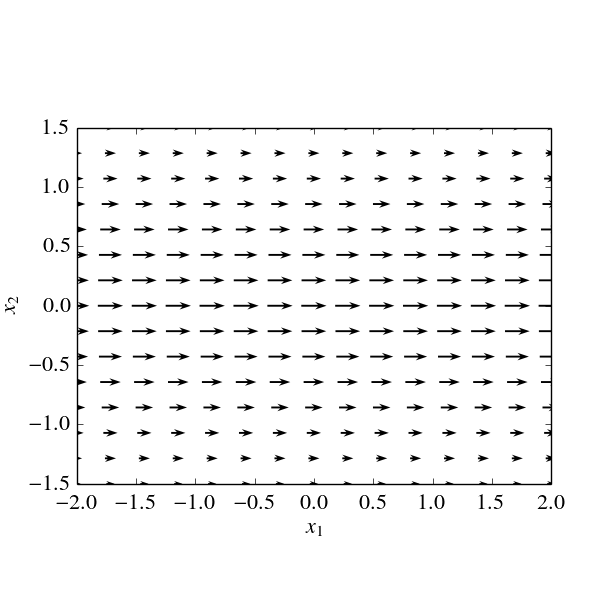
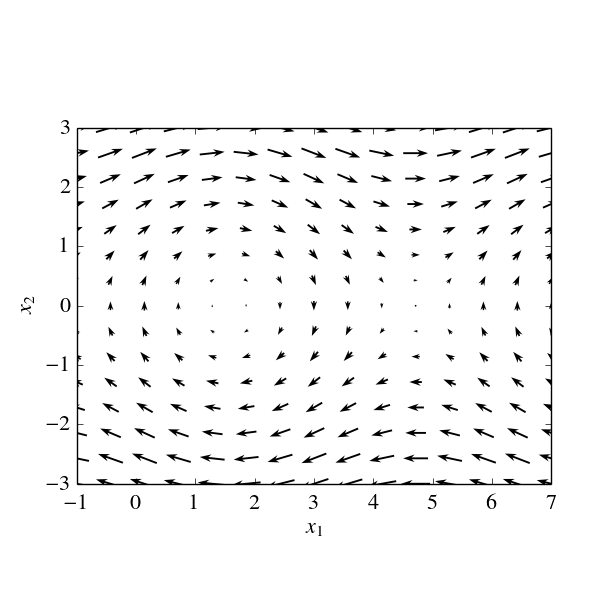
Figure 1: Left: river drift. Right: pendulum drift.

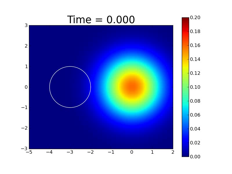
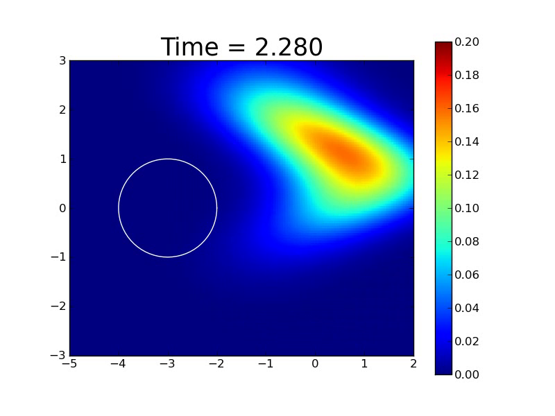
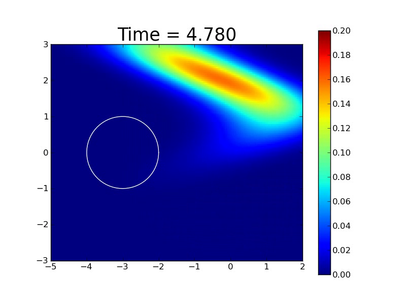
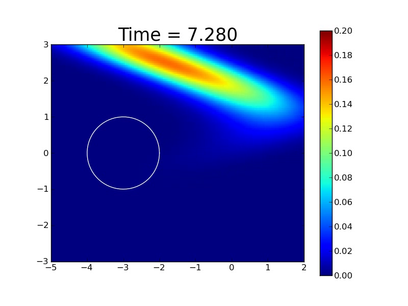
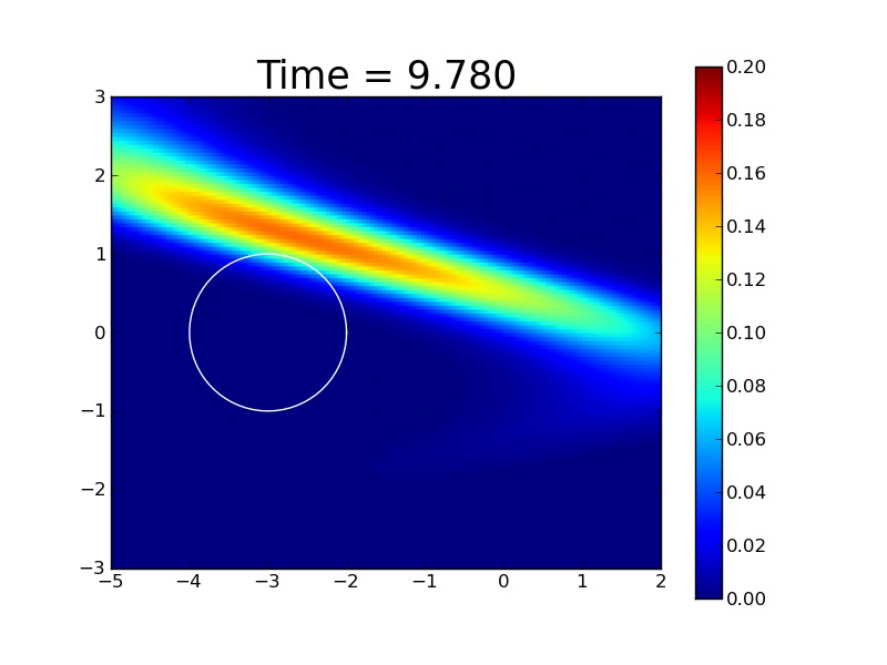
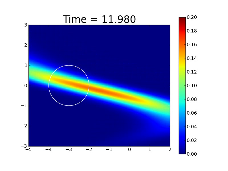
Figure 2: Trajectory for the boat problem computed by the algorithm.

Assume that the speed of the river water is given by

$$\mathbf{v}_{0}(x)=\begin{pmatrix}\alpha+e^{-\beta x_{2}^{2}}\\ 0\end{pmatrix},$$

the island is a unit circle centered at $x_{0}$, the initial position of the boat is described by the density function

$$\rho_{0}(x)=\frac{1}{2\pi\sigma^{2}}\,e^{-|x|^{2}/(2\sigma^{2})}.$$ (4.1)

Thus, the boat’s position $x(t)$ evolves according to the differential equation

$$\dot{x}=\mathbf{v}_{0}(x)+u,$$

where $u\in\mathbb{R}^{2}$ is a component of the boat’s velocity due to rowing. Here $|u|\leq u_{\text{max}}$.

Parameters for the computation: $\sigma=1$, $\alpha=\beta=0.5$, $u_{\text{max}}=0.75$, $x_{0}=(-3,0)$, $T=12$.

4.2 Pendulum

Here we want to stop a moving pendulum whose initial position is uncertain. In this case we have

$$\mathbf{v}_{0}(x)=\begin{pmatrix}x_{2}\\ \cos x_{1}\end{pmatrix},\qquad\mathbf{v}_{1}(x)=\begin{pmatrix}1\\ 0\end{pmatrix}.$$

Hence the control system takes the form

$$\dot{x}=\mathbf{v}_{0}(x)+u\,\mathbf{v}_{1}(x),$$

where $u\in[-u_{\text{max}},u_{\text{max}}]$ is an external force. The initial position of the pendulum is given by (4.1). The target is a unit circle centered at $(\pi/2,0)$.

Parameters for the computation: $\sigma=1$, $u_{\text{max}}=0.5$, $x_{0}=(\pi/2,0)$, $T=6$.

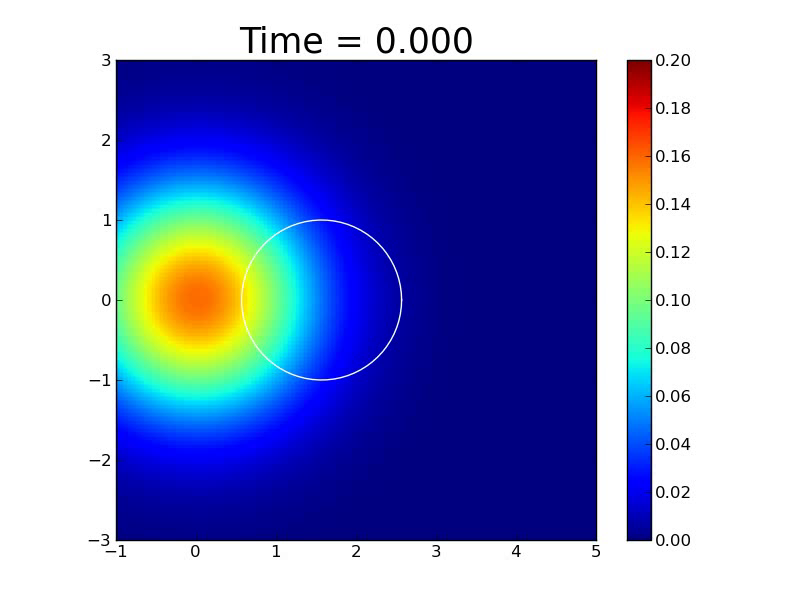
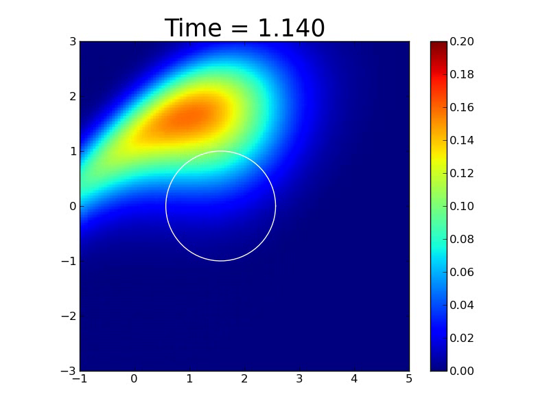
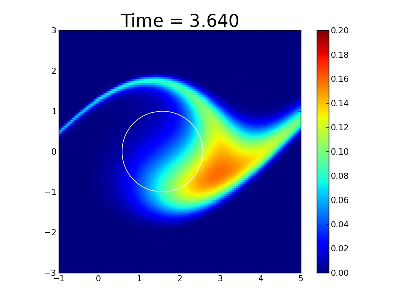
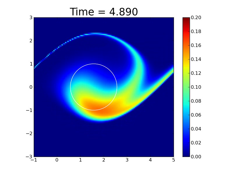
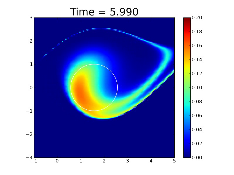
Figure 3: Trajectory for the pendulum problem computed by the algorithm.

4.3 Sheep

Consider a herd of sheep located near the origin. The sheep are effected by a vector field $v_{0}(x)$ pushing them away from the origin. To prevent this we can turn on repellers, which are located at the following positions

$$x_{k}=\left(R\cos\frac{2\pi(k-1)}{m},R\sin\frac{2\pi(k-1)}{m}\right),\qquad k=1,\ldots,m.$$

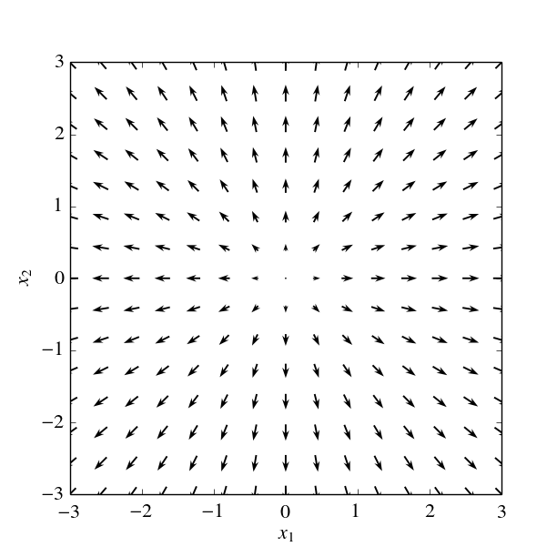
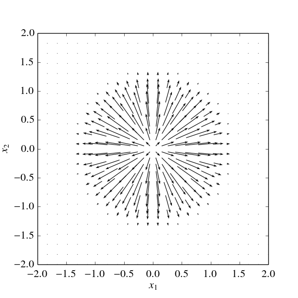
Figure 4: Left: sheep drift. Right: repeller’s force field.

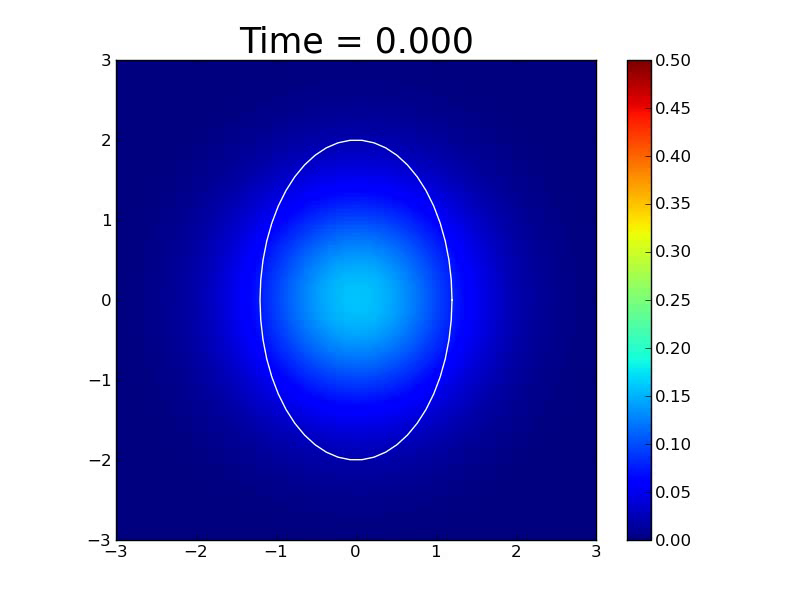
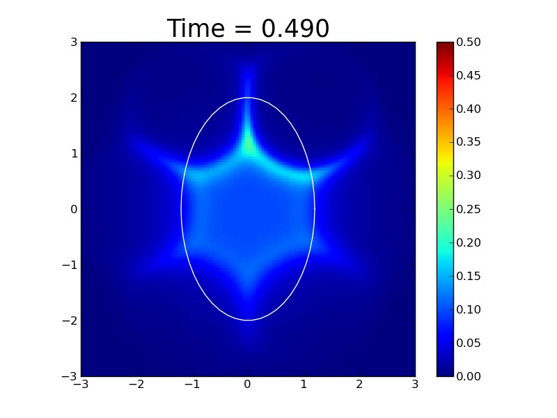
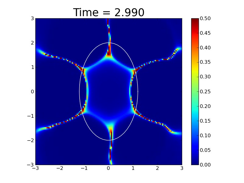
Figure 5: Trajectory for the sheep problem computed by the algorithm.

Each repeller produces a vector field $\mathbf{v}_{k}(x)$. So we have

$$\mathbf{v}(x,u)=\mathbf{v}_{0}(x)+\sum_{k=1}^{m}u_{k}\mathbf{v}_{k}(x),$$

where $u_{k}$ is an intensity of $k$-th repeller. The control $u=(u_{1},\ldots,u_{m})$ belongs to the simplex

$$U=\left\{(u_{1},\ldots,u_{m})\;\colon\;\sum_{k=1}^{m}u_{k}=1,\,u_{k}\in[0,1],\;k=1,\ldots,m\right\}.$$

In what follows we set

$$\mathbf{v}_{0}(x)=\alpha\,\frac{x-x_{0}}{\sqrt{1+|x-x_{0}|^{2}}},$$

where $x_{0}$ is a certain point not far from the origin, and

$$\mathbf{v}_{k}(x)=\beta\,e^{-|x-x_{k}|^{4}}(x-x_{k}),\qquad k=1,\ldots,m.$$

Suppose that the initial distribution is given by (4.1), the target is an ellipse centered at $x_{0}$ whose major and minor semi-axes are $a$ and $b$.

Parameters for the computation: $\sigma=1$, $x_{0}=(0,0)$, $T=3$, $m=6$, $a=2$, $b=1.2$.

Remark 4.1.

The answer to the minimization problem

$$\sum_{i=1}^{m}c_{i}\omega_{i}\to\min,\quad\omega\in U,$$

arising in the second step of the algorithm, is very simple. Let $j$ be such that

$$c_{j}\leq c_{i}\quad\mbox{for all }i=1,\ldots,m;$$

then an optimal solution is given by $\bar{\omega}=(0,\ldots,0,1,0,\ldots,0)$, where $1$ is located at the $j$-th position. In particular, this means that at every time moment $t$ only one repeller is turned on. Hence instead of repellers, we may think of a dog that jumps from one place to another.

Acknowledgements

The work was supported by the Russian Science Foundation, grant No 17-11-01093.

References

• [1] N.Β Pogodaev. Optimal control of continuity equations. NoDEA, Nonlinear Differ. Equ. Appl., 23(2):24, 2016.
• [2] S.Β Roy and A.Β BorzΓ¬. Numerical investigation of a class of liouville control problems. Journal of Scientific Computing, Mar 2017.
• [3] V.Β A. Srochko. Iterative methods for solving optimal control problems. Fizmatlit, Moscow, 2000.
• [4] L.Β W. Tu. An introduction to manifolds. 2nd revised ed. 2nd ed. New York, NY: Springer, 2nd ed. edition, 2011.