Line defect Schur indices, Verlinde algebras and $U(1)_{r}$ fixed points

Abstract

Given an ${\mathcal{N}}=2$ superconformal field theory, we reconsider the Schur index ${\mathcal{I}}_{L}(q)$ in the presence of a half line defect $L$. Recently Cordova-Gaiotto-Shao found that ${\mathcal{I}}_{L}(q)$ admits an expansion in terms of characters of the chiral algebra ${\mathcal{A}}$ introduced by Beem et al., with simple coefficients $v_{L,\beta}(q)$. We report a puzzling new feature of this expansion: the $q\to 1$ limit of the coefficients $v_{L_{,}\beta}(q)$ is linearly related to the vacuum expectation values $\langle L\rangle$ in $U(1)_{r}$-invariant vacua of the theory compactified on $S^{1}$. This relation can be expressed algebraically as a commutative diagram involving three algebras: the algebra generated by line defects, the algebra of functions on $U(1)_{r}$-invariant vacua, and a Verlinde-like algebra associated to ${\mathcal{A}}$. Our evidence is experimental, by direct computation in the Argyres-Douglas theories of type $(A_{1},A_{2})$, $(A_{1},A_{4})$, $(A_{1},A_{6})$, $(A_{1},D_{3})$ and $(A_{1},D_{5})$. In the latter two theories, which have flavor symmetries, the Verlinde-like algebra which appears is a new deformation of algebras previously considered.

1 Introduction

This paper describes a puzzling new feature of the line defect Schur index in ${\mathcal{N}}=2$ theories, introduced in Dimofte:2011py and recently reconsidered in Cordova:2016uwk . In short, there is an unexpectedly close relation between:

• the Schur index in the presence of a supersymmetric (half) line defect $L$,

• the vevs $\langle L\rangle$ in $U(1)_{r}$-invariant vacua of the theory compactified on $S^{1}$.

The precise statements and some discussion appear in §1.7-§1.9 below; the intervening sections provide the necessary notation and background.

1.1 Schur indices and chiral algebras

In Beem:2013sza a novel correspondence between 4d $\mathcal{N}=2$ SCFT and 2d chiral algebras was discovered: given an ${\mathcal{N}}=2$ SCFT, there is a corresponding chiral algebra ${\mathcal{A}}$. The operators in the vacuum module of the chiral algebra ${\mathcal{A}}$ correspond to local operators in the original ${\mathcal{N}}=2$ theory which contribute to the Schur index ${\mathcal{I}}(q)$ (and Macdonald index).

The algebras ${\mathcal{A}}$ corresponding to Argyres-Douglas theories have been intensively studied in e.g. Beem:2013sza ; Beem:2014zpa ; Buican:2015ina ; Cordova:2015nma ; Creutzig:2017qyf ; Song:2017oew ; Xie:2016evu ; Buican:2017uka . In particular, the chiral algebra for the $(A_{1},A_{2N})$ Argyres-Douglas theory was conjectured to be the Virasoro minimal model with $(p,q)=(2,2N+3)$, and the chiral algebra for $(A_{1},D_{2N+1})$ Argyres-Douglas theories was conjectured to be $\widehat{\mathfrak{sl}(2)}_{k}$ at level $k=-4N/(2N+1)$. The Schur indices for certain Argyres-Douglas theories have been computed and indeed match the vacuum characters of the corresponding 2d chiral algebra Buican:2015ina ; Cordova:2015nma ; Cordova:2016uwk ; Buican:2017uka .

1.2 Schur indices with half line defects and Verlinde algebra

In Cordova:2016uwk this story was extended to include the non-vacuum characters of the chiral algebra ${\mathcal{A}}$, by considering a new Schur index ${\mathcal{I}}_{L}(q)$, which counts operators of the ${\mathcal{N}}=2$ SCFT which sit at the endpoint of a supersymmetric “half line defect” $L$. In various examples, Cordova:2016uwk found that ${\mathcal{I}}_{L}(q)$ can be expressed as a linear combination of characters associated to modules for the algebra ${\mathcal{A}}$:

$${\mathcal{I}}_{L}(q)=\sum_{\beta}v_{L,\beta}(q)\chi_{\beta}(q)$$ (1)

where $\chi_{\beta}(q)$ are the characters, and $v_{L,\beta}(q)$ are some simple Laurent polynomials in $q$, with integer coefficients.

In the expansion (1), the index $\beta$ is running over some finite collection of modules, which moreover are closed under a canonical action of the modular $S$ matrix. This being so, we can use the Verlinde formula to define a commutative and associative algebra ${\mathcal{V}}$, generated by the “primaries” $\Phi_{\beta}$ corresponding to the modules with characters $\chi_{\beta}(q)$, with product laws of the form

$$[\Phi_{\beta}]\times[\Phi_{\alpha}]=c_{\beta\alpha}^{\gamma}[\Phi_{\gamma}].$$ (2)

In $(A_{1},A_{2N})$ Argyres-Douglas theories this commutative product corresponds to the true fusion operation in the $(2,2N+3)$ Virasoro minimal model. More generally though, we do not claim to interpret this product as any kind of fusion operation: we just use the formal rule provided by the Verlinde formula. In the following we will often refer to these product laws as modular fusion rules of the Verlinde-like algebra ${\mathcal{V}}$.

Now, let us return to the expansion (1) and specialize the coefficients $v_{L,\beta}(q)$ to $q=1$, defining

$$V_{L,\beta}=v_{L,\beta}(q=1).$$ (3)

Then for every line defect $L$ we get an element $f(L)\in{\mathcal{V}}$ by

$$f(L)=\sum_{\beta}V_{L,\beta}[\Phi_{\beta}].$$ (4)

Remarkably, Cordova:2016uwk found evidence that this map is actually a homomorphism of commutative algebras,

$$f:{\mathcal{L}}\to{\mathcal{V}}$$ (5)

where ${\mathcal{L}}$ is the commutative OPE algebra of line defects in the original ${\mathcal{N}}=2$ theory.

$f$ always maps the trivial line defect to the vacuum module, since the Schur index without any line defect insertions is the vacuum character of ${\mathcal{A}}$. Thus the fact that the trivial line defect is the identity in the OPE algebra gets mapped to the fact that the vacuum module is the identity in the Verlinde algebra ${\mathcal{V}}$.

Evidence for the homomorphism property of the line defect Schur index was observed in Cordova:2016uwk in the $(A_{1},A_{2})$ and $(A_{1},A_{4})$ theories. In §5.4 below we give evidence that the same is true in the $(A_{1},A_{6})$ theory. We also extend to the $(A_{1},D_{3})$ and $(A_{1},D_{5})$ theories, in §6.1 and §6.2, but this involves a little twist: see §1.8 below.

1.3 A simple example

Just to fix ideas, we quickly review here the case of the Argyres-Douglas theory of type $(A_{1},A_{2})$. The basic data are:

• There are five distinguished nontrivial line defects $L_{1},\dots,L_{5}$ in the theory, which generate all the rest by operator products. In fact one only needs products involving consecutive $L_{i}$: the most general simple line defect can be written Gaiotto:2010be

  $$L=L_{i}^{m}L_{i+1}^{n}$$ (6)

  for $i\in\{1,\dots,5\}$ and $m,n\geq 0$ (letting $L_{6}=L_{1}$). We also have the trivial line defect which we write as $1$.

• The chiral algebra ${\mathcal{A}}$ is the $(2,5)$ Virasoro minimal model, with $c=-22/5$. The corresponding Verlinde algebra ${\mathcal{V}}$ has two generators $[\Phi_{1,1}]$, $[\Phi_{1,2}]$ corresponding to the two primaries. $[\Phi_{1,1}]$ is the identity element, so the only nontrivial product is $[\Phi_{1,2}]\times[\Phi_{1,2}]$, which is

  $$[\Phi_{1,2}]\times[\Phi_{1,2}]=[\Phi_{1,1}]+[\Phi_{1,2}].$$ (7)

The line defect Schur indices come out to Cordova:2016uwk

$${\mathcal{I}}_{1}(q)=\chi_{1,1}(q),\qquad{\mathcal{I}}_{L_{i}}(q)=q^{-\frac{1}{2}}\big{(}\chi_{1,1}(q)-\chi_{1,2}(q)\big{)}.$$ (8)

Thus the homomorphism $f$ in this case is

$$f(1)=[\Phi_{1,1}],\qquad f(L_{i})=[\Phi_{1,1}]-[\Phi_{1,2}].$$ (9)

In particular, $f$ forgets the index $i$, so it identifies the $5$ generators $L_{i}$. Moreover, $f$ collapses the infinite-dimensional algebra ${\mathcal{L}}$, spanned by the operators (6), down to the two-dimensional algebra ${\mathcal{V}}$.

1.4 Diagonalizing the Verlinde algebra

To explain the main new results of this paper, we need a brief digression to recall a structural fact about the Verlinde algebra ${\mathcal{V}}$: the modular $S$ operator gives a canonical diagonalization of ${\mathcal{V}}$ Verlinde:1988sn . Concretely, if we choose an ordering of the $n$ primaries, then we can represent the operation of fusion with $\Phi_{i}$ by an $n\times n$ matrix $N_{\Phi_{i}}$, and likewise $S$ by an $n\times n$ matrix; then the statement is that the matrices

$$\hat{N}_{\Phi}=SN_{\Phi}S^{-1}$$ (10)

are all diagonal.

For example, in the $(2,5)$ Virasoro minimal model, if we choose the ordering of the primaries $(\Phi_{1,1},\Phi_{1,2})$, then we have D.Francesco

$$N_{\Phi_{1,1}}=\begin{pmatrix}1&0\\ 0&1\end{pmatrix},\quad N_{\Phi_{1,2}}=\begin{pmatrix}0&1\\ 1&1\end{pmatrix},\quad S=\frac{2}{\sqrt{5}}\begin{pmatrix}-\sin\frac{2\pi}{5}&\sin\frac{4\pi}{5}\\ \sin\frac{4\pi}{5}&\sin\frac{2\pi}{5}\end{pmatrix},$$ (11)

from which we can compute

$$\hat{N}_{\Phi_{1,1}}=\begin{pmatrix}1&0\\ 0&1\end{pmatrix},\quad\hat{N}_{\Phi_{1,2}}=\begin{pmatrix}\frac{1-\sqrt{5}}{2}&0\\ 0&\frac{1+\sqrt{5}}{2}\end{pmatrix}.$$ (12)

The representation of ${\mathcal{V}}$ by the diagonal matrices $\hat{N}_{\Phi}$ shows that ${\mathcal{V}}$ is naturally isomorphic to a direct sum of copies of ${\mathbb{C}}$. Moreover these copies correspond canonically to the primaries themselves, using the ordering of the primaries we have chosen. Another way of saying this is: ${\mathcal{V}}$ is canonically isomorphic to the algebra of functions on the set of primaries of ${\mathcal{A}}$. We will use the statement in this form, in §1.5 below.

1.5 Verlinde algebra and $U(1)_{r}$-fixed points in three dimensions

Now we recall another place where the Verlinde algebra of ${\mathcal{A}}$ has recently appeared.

We consider the compactification of our superconformal ${\mathcal{N}}=2$ theory to three dimensions on $S^{1}$. As is well known, beginning with Seiberg:1996nz , the Coulomb branch of the compactified theory is a hyperkähler space ${\mathcal{N}}$. For example, if our theory is a theory of class ${\mathcal{S}}$, say ${\mathcal{S}}[{\mathfrak{g}},C]$, then ${\mathcal{N}}$ is a moduli space of solutions of Hitchin equations on $C$ with gauge algebra ${\mathfrak{g}}$ Gaiotto:2009hg ; MR89a:32021 .

The $U(1)_{r}$ symmetry of the theory acts geometrically on ${\mathcal{N}}$. This action is an important tool in the study of this space. For example, it can be used to compute the Betti numbers of the Hitchin moduli spaces, as was noted already in MR89a:32021 . More recently Gukov:2015sna ; Gukov:2016lki this $U(1)_{r}$ action has been used to define and compute a new “$U(1)_{r}$-equivariant index” for ${\mathcal{N}}$, related to a Coulomb branch index in the ${\mathcal{N}}=2$ theory. In both computations the starring role is played by the fixed locus $F\subset{\mathcal{N}}$ of the $U(1)_{r}$ symmetry. The points of $F$ are the $U(1)_{r}$-invariant vacua of the compactified theory.

For our purposes the key fact about $F$ is the following recent observation: the points of $F$ are naturally in 1-1 correspondence with the primaries of ${\mathcal{A}}$ Cecotti:2010fi ; Fredrickson-Neitzke ; Fredrickson-talk ; Fredrickson:2017yka . Combining this correspondence with the picture of ${\mathcal{V}}$ reviewed in §1.4, we conclude that there is a canonical isomorphism

$$h:{\mathcal{V}}\to{\mathcal{O}}(F),$$ (13)

where ${\mathcal{O}}(F)$ means the algebra of functions on $F$. Concretely, $h$ maps $[\Phi]$ to the vector of diagonal entries of $\hat{N}_{\Phi}$, using the correspondence above to match up the points of $F$ with the positions along the diagonal.

1.6 Fixed points and vevs

We consider the vacuum expectation values of ${\frac{1}{2}}$-BPS line defects wrapped around $S^{1}$ in $S^{1}\times{\mathbb{R}}^{3}$. These vevs are functions on the vacuum moduli space ${\mathcal{N}}$; the process of taking vevs gives a homomorphism of commutative algebras

$${\mathcal{L}}\to{\mathcal{O}}({\mathcal{N}})$$ (14)

from the OPE algebra of ${\frac{1}{2}}$-BPS line defects to the algebra ${\mathcal{O}}({\mathcal{N}})$ of holomorphic functions on ${\mathcal{N}}$. Now consider the restriction of these vevs to the $U(1)_{r}$-fixed locus $F\subset{\mathcal{N}}$: this gives another homomorphism of commutative algebras,

$$g:{\mathcal{L}}\to{\mathcal{O}}(F).$$ (15)

In Argyres-Douglas theories, the map $g$ is very far from being an isomorphism: it forgets most of the details of a line defect, remembering only its vevs at the finitely many $U(1)_{r}$-invariant vacua. This is reminiscent of the fact that the map $f$, built from line defect Schur indices ${\mathcal{I}}_{L}$, likewise forgets most of the details of the line defects $L$. In the next section we flesh this out into a precise sense in which $f$ and $g$ are “the same.”

Before we state our main result, we would like to point out that the ${\frac{1}{2}}$-BPS line defects that we are talking about in this section are full line defects, which are by definition different from the half line defects in 1.2. However, away from the endpoints of the half line defects they are “locally” the same object. In particular the OPE algebra of half line defects is isomorphic to the OPE algebra of full line defects, both of which we denote as ${\mathcal{L}}$.

1.7 The commutative diagram

So far in this introduction we have described three a priori unrelated commutative algebras associated to an ${\mathcal{N}}=2$ SCFT:

• The OPE algebra ${\mathcal{L}}$ of ${\frac{1}{2}}$-BPS line defects,

• The Verlinde algebra ${\mathcal{V}}$ associated to the chiral algebra ${\mathcal{A}}$,

• The algebra ${\mathcal{O}}(F)$ of functions on the set of $U(1)_{r}$-invariant vacua of the theory compactified on $S^{1}$.

We also described three a priori unrelated maps between these algebras:

• The map $f:{\mathcal{L}}\to{\mathcal{V}}$ obtained by computing Schur indices in the presence of half line defects and expanding them in terms of characters of ${\mathcal{A}}$,

• The isomorphism $h:{\mathcal{V}}\to{\mathcal{O}}(F)$, constructed using the mysterious identification between $U(1)_{r}$-invariant vacua and chiral primaries, and using also the modular $S$ matrix,

• The map $g:{\mathcal{L}}\to{\mathcal{O}}(F)$ obtained by compactifying the theory on $S^{1}$ and evaluating line defect vevs in $U(1)_{r}$-invariant vacua of the reduced theory.

These ingredients can be naturally assembled into a diagram:

This raises the natural question of whether the diagram commutes, i.e. whether

$$h\circ f=g.$$ (16)

In §5 below, we verify by direct computation that (16) indeed holds, in the Argyres-Douglas theories of type $(A_{1},A_{2})$, $(A_{1},A_{4})$, and $(A_{1},A_{6})$. In §6 we verify a similar statement in $(A_{1},D_{3})$ and $(A_{1},D_{5})$ theories: see §1.8 below for more on this.

The commutativity (16) is the main new result of this paper. In a sense it is not surprising — once you realize that this diagram exists, it is hard to imagine that it would not commute — but on the other hand its physical meaning is not at all transparent, at least to us. It should be interesting to unravel. We comment a bit further on this question in §1.9 below.

1.8 Flavor symmetries

In ${\mathcal{N}}=2$ theories with flavor symmetries the story described above can be enriched. The Schur index, rather than being a function ${\mathcal{I}}_{L}(q)$, is promoted to ${\mathcal{I}}_{L}(q,z)$ where $z$ stands for the flavor fugacities. The chiral algebra ${\mathcal{A}}$ also contains currents for the flavor symmetry group, and thus its characters are promoted to $\chi_{i}(q,z)$. It is natural to ask whether there are analogues of the homomorphisms $f$, $g$, $h$ in such theories with the extra parameters $z$ included.

In §6 below we consider this question for the $(A_{1},D_{3})$ and $(A_{1},D_{5})$ Argyres-Douglas theories, which have flavor symmetry $SU(2)$. The Cartan subgroup of $SU(2)$ consists of matrices $diag(z,z^{-1})$ for $\lvert z\rvert=1$; thus the fugacity in this case is just a single number $z$. The chiral algebras in these theories are ${\mathcal{A}}=\widehat{\mathfrak{sl}(2)}_{-\frac{4}{3}}$ and ${\mathcal{A}}=\widehat{\mathfrak{sl}(2)}_{-\frac{8}{5}}$ respectively.

In the compactification of the theory on $S^{1}$, turning on the fugacity $z$, with $\lvert z\rvert=1$, corresponds to switching on a “flavor Wilson line” around the $S^{1}$. Such a Wilson line leads to a deformation of ${\mathcal{N}}$ which does not break the $U(1)_{r}$ symmetry. Thus for any fixed $z$ we can consider the fixed locus $F_{z}\subset{\mathcal{N}}_{z}$, which turns out to be discrete, just as in the $(A_{1},A_{2n})$ theories we considered above. Evaluating line defect vevs at $F_{z}$ we get a homomorphism

$$g_{z}:{\mathcal{L}}\to{\mathcal{O}}(F_{z}).$$ (17)

Now we would like to repeat the story of §1.7 here, i.e. to construct maps $f_{z}$ and $h_{z}$, and to verify (16). A key question arises: what should we use as “Verlinde algebra”? There are no conventional two-dimensional conformal field theories with ${\mathcal{A}}$ as symmetry algebras; the usual candidate with symmetry $\widehat{\mathfrak{sl}(2)}_{k}$ would be the WZW model, but that only makes sense for positive integer $k$. Thus there is no clear physically-defined notion of Verlinde algebra. Still, it was realized in V.G.Kac that at admissible levels there is a finite set of admissible representations of ${\mathcal{A}}$ whose characters span a representation of the modular group $SL(2,{\mathbb{Z}})$. A Verlinde-like algebra built from the admissible representations ${\mathcal{V}}_{1}$ was constructed in Koh-Sorba where the fusion rules were given by naive application of the Verlinde formula V.G.Kac . ${\mathcal{V}}_{1}$ has the odd feature that some of the structure constants are equal to $-1$.

Nevertheless, we could try to construct $f_{z}$ and $h_{z}$, and verify (16), using this algebra ${\mathcal{V}}_{1}$. What we find experimentally in §6 below is that this does not quite work: we need to use a deformed Verlinde-like algebra ${\mathcal{V}}_{z}$. ${\mathcal{V}}_{z}$ is obtained from ${\mathcal{V}}_{1}$ by replacing each structure constant $-1$ by $-z^{2}$. Once we make this modification, the whole story goes through as in §1.7 above.

1.9 Interpretations and comments

• The main new result of this paper is the commutative diagram in §1.7. What is the physical interpretation of this commutative diagram? One tempting possibility is that there is a new localization computation of the Schur index. Indeed, if we think of the Schur index as a kind of partition function on $S^{3}\times S^{1}$, we could imagine computing it by first reducing on $S^{1}$ and then making some computation in the resulting effective theory on $S^{3}$. After this reduction the line defects become local operators, which are determined by their vevs on ${\mathcal{N}}$. In a localization computation using $U(1)_{r}$, they could get further reduced to just their vevs in the $U(1)_{r}$-invariant vacua. This would match our observation that the object $f(L)$ — which contains much of the information of the Schur index ${\mathcal{I}}_{L}$ — is linearly related to $g(L)$, i.e. to the vevs of $L$ in the $U(1)_{r}$-invariant vacua.

• Our verification of the commutativity (16) requires us to evaluate explicitly the vacuum expectation values of ${\frac{1}{2}}$-BPS line defects at the fixed points of the $U(1)_{r}$ action on ${\mathcal{N}}$. In the language of the Hitchin system, this amounts to solving an instance of the nonabelian Hodge correspondence: for some specific Higgs bundles, we determine the corresponding complex flat connections up to equivalence. It would be very interesting to see how far one can push these ideas: can we compute the vevs in every case where the vacua are isolated? Can we extend beyond the fixed points, say to get some information about their infinitesimal neighborhoods? Can we say anything about non-isolated fixed points?

• It is natural to ask how broadly the commutative diagram of §1.7 exists; so far we have checked it only in five theories. We conjecture that it exists more generally whenever it makes sense, i.e. whenever the $U(1)_{r}$-invariant vacua of the theory reduced on $S^{1}$ are all isolated. The $U(1)_{r}$-invariant vacua are isolated in all Argyres-Douglas theories where the question has been investigated, e.g. the $(A_{m},A_{n})$ theories for $gcd(m+1,n+1)=1$, but more generally they are usually not isolated.

• One of the simplest examples where the $U(1)_{r}$-invariant vacua are not isolated is ${\mathcal{N}}=2$ super Yang-Mills with $G=SU(2)$ and $N_{f}=4$, compactified on $S^{1}$ with generic flavor Wilson lines. In this theory it appears that there are $4$ isolated $U(1)_{r}$-invariant vacua, but also an $S^{2}$ of $U(1)_{r}$-invariant vacua, as explained e.g. in hauselthesis . In this theory Fredrickson:2017yka argued that nevertheless there is a correspondence between connected components of the space of $U(1)_{r}$-invariant vacua and chiral primaries. It would be very interesting to understand how the diagram (16) can be extended to this case. (An obstacle to the most naive extension is that the line defect vevs are not constant on the $S^{2}$ of invariant vacua. Perhaps one needs instead to take the average over this $S^{2}$.)

• In this paper one of the main players is the homomorphism $f:{\mathcal{L}}\to{\mathcal{V}}$. The observation that there is some relation between algebras of line defects and Verlinde algebras was made already in Cecotti:2010fi . Indeed, that paper described a map $f^{\prime}:{\mathcal{L}}\to{\mathcal{V}}$ in the $(A_{1},A_{2N})$ theories, constructed in a different way, by mapping certain distinguished line defects directly to minimal model primaries. To forestall a possible confusion, we emphasize that $f$ and $f^{\prime}$ are not the same. For example, in the $(A_{1},A_{2})$ theory we have $f^{\prime}(L_{i})=[\Phi_{1,2}]$, while (9) says $f(L_{i})=[\Phi_{1,1}]-[\Phi_{1,2}]$.

• Beyond line defects one could also consider surface defects and interfaces between surface defects. The Schur index in the presence of surface defects, and its relation to 2d chiral algebra, were studied quite recently in Cordova:2017ohl ; Cordova:2017mhb and also featured in the ongoing work Beem-Peelaers-Rastelli . It might be interesting to incorporate surface defects into the story of this paper.

• In this paper we focused on examples of $(A_{1},A_{2N})$ and $(A_{1},D_{2N+1})$ Argyres-Douglas theories, mainly because their chiral algebras have been relatively well understood and computation of line defect generators is not too complicated. What about other $(A_{1},{\mathfrak{g}})$ Argyres-Douglas theories? There is one more example which we expect should be relatively straightforward, namely $(A_{1},D_{4})$, for which the chiral algebra is $\widehat{{\mathfrak{sl}}(3)}_{-3/2}$ Beem ; Rastelli ; Cordova:2015nma ; Buican:2015ina . Beyond this:

  • The chiral algebra for $(A_{1},A_{2N-1})$ Argyres-Douglas theories with $N>2$ is conjectured to be the $\mathcal{B}_{N+1}$ algebra, the subregular quantum Hamiltonian reduction of $\widehat{{\mathfrak{sl}}(N)}_{-N^{2}/(N+1)}$ Creutzig:2017qyf ; Beem:2017ooy . As pointed out in Fredrickson:2017yka , the relevant modules associated with the $U(1)_{r}$ fixed points depend on the parity of $N$, and for even $N$, the relevant modules are suitable representatives of local modules which are closed under modular transformation Auger-Creutzig-Kanade-Rupert ; Creutzig:2017qyf ; Beem:2017ooy ; Beem-Peelaers . For odd $N$, $S$-transformation turns local modules into twisted modules Auger-Creutzig-Kanade-Rupert ; Creutzig:2017qyf ; Beem:2017ooy ; Beem-Peelaers , which makes the matching of $U(1)_{r}$ fixed points with relevant modules very subtle Fredrickson:2017yka . These local and twisted modules and their modular properties are studied in Beem-Peelaers ; Beem:2017ooy ; Auger-Creutzig-Kanade-Rupert .

  • The situation is similar for $(A_{1},D_{2N})$ Argyres-Douglas theories with $N>2$. Here the chiral algebra has been conjectured to be the $\mathcal{W}_{N}$ algebra coming from a non-regular quantum Hamiltonian reduction of $\widehat{{\mathfrak{sl}}(N+1)}_{-(N^{2}-1)/N}$ Creutzig:2017qyf . For even $N$, Fredrickson:2017yka confirmed that the relevant modules are suitable representatives of local modules listed in Creutzig:2017qyf , while for odd $N$ the situation becomes subtle again Fredrickson:2017yka since $S$-transformation turns local modules into twisted modules Creutzig:2017qyf .

  • Chiral algebras for $(A_{1},E_{6,7,8})$ Argyres-Douglas theories were conjectured in Cordova:2015nma ; Song:2017oew , and at least for $(A_{1},E_{6})$ and $(A_{1},E_{8})$ there is a natural guess for the relevant class of modules. However, in these theories the computation of line defect generators and their framed BPS spectra has not been worked out; it would be interesting to develop it.

2 Schur indices and their IR formulas

In this section we review the definition and IR formula for the ordinary Schur index and the Schur index with half line defects inserted.

2.1 The Schur index

The superconformal index of a four-dimensional $\mathcal{N}=2$ SCFT is defined as Kinney:2005ej ; Gadde:2011uv

$${\mathcal{I}}(p,q,t,a_{i})=\text{Tr}(-1)^{F}p^{j_{2}-j_{1}-r}q^{j_{2}+j_{1}-r}t^{R+r}\prod_{i}a_{i}^{f_{i}}e^{-\beta\delta_{2\dot{-}}},$$ (18)

where

$$2\delta_{2\dot{-}}=\{\widetilde{Q}_{2\dot{-}},\widetilde{Q}^{\dagger}_{2\dot{-}}\}=E-2j_{2}-2R+r.$$ (19)

Here $p,q,t$ are three superconformal fugacities, $a_{i}$ are flavor symmetry fugacities, $E$ is the scaling dimension, $j_{1}$ and $j_{2}$ are Cartan generators of $SU(2)_{1}\times SU(2)_{2}$, $R$ and $r$ are the Cartan generators of the $SU(2)_{R}\times U(1)_{r}$ $R$-symmetry group. The trace is taken over the Hilbert space on $S^{3}$ in radial quantization.

The Schur index is obtained by taking the $q=t$ limit Gadde:2011ik ; Gadde:2011uv ,

$${\mathcal{I}}(q,a_{i})=\text{Tr}(-1)^{F}q^{E-R}\prod_{i}a_{i}^{f_{i}}.$$ (20)

Here the contributing states are $\frac{1}{4}$-BPS, annihilated by four supercharges: $Q^{1}_{-}$, $\tilde{Q}_{2\dot{-}}$, $S_{1}^{-}$ and $\tilde{S}^{2\dot{-}}$. Their quantum numbers satisfy

$$E-j_{1}-j_{2}-2R=0,\quad j_{1}-j_{2}+r=0.$$ (21)

2.2 The IR formula for the Schur index

Recently an IR formula for the Schur index was conjectured in Cordova:2015nma , relating the Schur index to the trace of the “quantum monodromy” operator, a $q$-series introduced in Cecotti:2010fi :

$${\mathcal{I}}(q)=(q)_{\infty}^{2r}\text{Tr}[M(q)],\quad(q)_{\infty}:=\prod_{j=0}^{\infty}(1-q^{j+1}).$$ (22)

In this section we review the mechanics of this formula.

To write down the operator $M(q)$, we need to perturb to a point of the Coulomb branch of the theory, where the only massless fields are those of abelian ${\mathcal{N}}=2$ gauge theory. $M(q)$ will be built out of the massive BPS spectrum of the theory.

Recall that massive BPS states in an ${\mathcal{N}}=2$ theory lie in representations of $SU(2)_{J}\times SU(2)_{R}$, where $SU(2)_{J}$ is the little group. The one-particle Hilbert space is graded by the IR charge lattice $\Gamma$, consisting of electromagnetic and flavor charges: thus ${\mathcal{H}}=\oplus_{\gamma\in\Gamma}{\mathcal{H}}_{\gamma}$. Factoring out the center-of-mass degrees of freedom, we have:

$$\mathcal{H}_{\gamma}=[(2,1)\oplus(1,2)]\otimes h_{\gamma}.$$ (23)

To count BPS particles refined by representations of $SU(2)_{J}\times SU(2)_{R}$, one consider the protected spin character Gaiotto:2008cd

$$\operatorname{Tr}_{h_{\gamma}}[y^{J}(-y)^{R}]=\displaystyle\sum\limits_{n\in\mathbb{Z}}\Omega_{n}(\gamma)y^{n},$$ (24)

with integers $\Omega_{n}(\gamma)\in{\mathbb{Z}}$, and packages the $\Omega_{n}(\gamma)$ into the “Kontsevich-Soibelman factor”:

$$K(q;X_{\gamma};\Omega_{i}(\gamma)):=\prod_{n\in\mathbb{Z}}E_{q}((-1)^{n}q^{n/2}X_{\gamma})^{(-1)^{n}\Omega_{n}(\gamma)}.$$ (25)

$K$ is a $q$-series valued in the algebra of formal variables $X_{\gamma}$; these variables themselves are valued in the “quantum torus” algebra, obeying the relations

$$X_{\gamma}X_{\gamma^{\prime}}=q^{\langle\gamma^{\prime},\gamma\rangle}X_{\gamma^{\prime}}X_{\gamma}=q^{\frac{1}{2}\langle\gamma,\gamma^{\prime}\rangle}X_{\gamma+\gamma^{\prime}},$$ (26)

where $\langle,\rangle$ is the Dirac pairing on $\Gamma$. $E_{q}(z)$ is the quantum dilogarithm defined as

$$E_{q}(z)=\prod_{j=0}^{\infty}(1+q^{j+\frac{1}{2}}z)^{-1}=\displaystyle\sum\limits_{n=0}^{\infty}\frac{(-q^{\frac{1}{2}}z)^{n}}{(q)_{n}}.$$ (27)

The quantum monodromy operator $M(q)$ is defined as

$$M(q)=\prod_{\gamma\in\Gamma}^{\curvearrowleft}K(q;X_{\gamma};\Omega_{i}(\gamma)).$$ (28)

The ordering in this product is based on the central charges $Z_{\gamma}$: if $\text{arg}(Z_{\gamma_{1}})>\text{arg}(Z_{\gamma_{2}})$ then $K(X_{\gamma_{1}})$ is to the right of $K(X_{\gamma_{2}})$. The flavor charges — which have zero Dirac pairing with other charges — form a sublattice $\Gamma_{f}\subset\Gamma$. The trace operation is defined by a truncation to this sublattice:

$$\text{Tr}(X_{\gamma})=\begin{cases}0&\text{if}\quad\gamma\notin\Gamma_{f},\\ X_{\gamma}&\text{otherwise}.\end{cases}$$ (29)

If we denote a basis for $\Gamma_{f}$ by $(\gamma_{f_{a}})$, then the trace is a function of the $X_{\gamma_{f_{a}}}$, which are related to the flavor fugacities $a_{i}$ in the UV definition of the Schur index Cordova:2015nma ; Cordova:2016uwk .

$\operatorname{Tr}M(q)$ is invariant when crossing walls of marginal stability in the Coulomb branch Gaiotto:2008cd ; Kontsevich:2008fj ; Gaiotto:2009hg ; Dimofte:2009tm . Of course this is a necessity for (22) to make sense, since ${\mathcal{I}}(q)$ is defined directly in the UV and does not depend on a point of the Coulomb branch.

As pointed out in Cordova:2015nma ; Cordova:2016uwk , (22) is only a formal definition: in principle, in evaluating it, we could meet infinitely many terms contributing to the same power of $q$. In practice we may hope that these infinitely many terms will come with alternating signs so that they leave a well-defined Laurent series in $q$, but at least we need to have some definite prescription for how we will order the terms. In Cordova:2016uwk the authors propose a prescription to tackle this problem. First they rewrite (22) as

$${\mathcal{I}}(q)=(q)_{\infty}^{2r}\text{Tr}[S(q)\overline{S}(q)],$$ (30)

where $S(q)$ is the “quantum spectrum generator” (so called because it contains enough information to reconstruct the full BPS spectrum),

$$S(q)=\prod_{\text{arg}(Z_{\gamma})\in[0,\pi)}^{\curvearrowleft}K(q;X_{\gamma};\Omega_{i}(\gamma)),\quad\overline{S}(q)=\prod_{\text{arg}(Z_{\gamma})\in[\pi,2\pi)}^{\curvearrowleft}K(q;X_{\gamma};\Omega_{i}(\gamma)).$$ (31)

Next, they conjecture that $S(q)$ and $\overline{S}(q)$ can be expanded as Taylor series in $q$, with no negative powers of $q$ appearing. If this is so, then one can try to compute the coefficient of $q^{k}$ in $\operatorname{Tr}M(q)$ by expanding $S(q)$ and $\overline{S}(q)$ up to some large finite order $q^{N}$. The conjecture is that for large enough $N$ the coefficient of $q^{k}$ will stabilize to some limiting value (in the examples investigated in Cordova:2016uwk it is sufficient to take $N$ larger than some theory-dependent linear function of $k$.) In the examples we consider in this paper, we find that the necessary stabilization does indeed occur, and thus we can use the prescription of Cordova:2016uwk .

2.3 The Schur index with half line defects

Supersymmetric line defects in ${\mathcal{N}}=2$ theories have been studied extensively: a small sampling of references is Drukker:2009id ; Drukker:2009tz ; Gaiotto:2010be ; Cordova:2013bza ; Cordova:2016uwk .

The line defects which have been studied most extensively are full line defects. These are ${\frac{1}{2}}$-BPS objects extended along a straight line in some fixed direction $n^{\mu}\in\mathbb{R}^{4}$. For example, there are ${\frac{1}{2}}$-BPS line defects that extend along the time direction and sits at a point in $\mathbb{R}^{3}$, preserving four Poincaré supercharges, time translation, $SU(2)_{J}$ rotation around the defect in $\mathbb{R}^{3}$, and $SU(2)_{R}$ $R$-symmetry. The choices of half-BPS subalgebra which can be preserved by such a line defect are parameterized by $\zeta\in\mathbb{C}^{\times}$. When $\lvert\zeta\rvert=1$, so that $\zeta={\mathrm{e}}^{-{\mathrm{i}}\theta}$, the line defect can be interpreted as a heavy external BPS source particle, whose central charge has phase $\theta$.

In this section, following Cordova:2016uwk , we will be interested in half line defects in superconformal ${\mathcal{N}}=2$ theories. A half line defect extends along a ray in $\mathbb{R}^{4}$ and terminates at a point, say the origin. The half line defect looks like a full line defect except near its endpoint; in particular, the indexing set labeling half line defects is the same as that for full line defects, and it will sometimes be convenient to let the symbol $L$ stand simultaneously for a half line defect and for its corresponding full line defect. The endpoint, however, only preserves two Poincaré supercharges, and breaks all translation symmetry. Moreover the endpoint supports a variety of local endpoint operators; these are the operators which will be counted by the line defect Schur index.

More generally we can consider a junction of multiple half line defects $L_{i}$. To preserve some common supersymmetry, these half line defects must lie in a common spatial plane ${\mathbb{R}}^{2}\subset{\mathbb{R}}^{3}$. Each $L_{i}$ ends at the origin and has orientation

$$n_{i}^{\mu}=(\cos\theta_{i},\sin\theta_{i},0,0),$$ (32)

where $\theta_{i}$ is the phase of the central charge of $L_{i}$. After conformal mapping to $S^{3}\times S^{1}$, each half line defect wraps $S^{1}$ and sits at a point on a common great circle on $S^{3}$. This configuration preserves one Poincaré supercharge and one conformal supercharge,

$$Q=Q^{1}_{-}+\tilde{Q}_{2\dot{-}},\quad S=S_{1}^{-}+\tilde{S}^{2\dot{-}}.$$ (33)

Recall from Gadde:2011uv that $Q^{1}_{-}$, $\tilde{Q}_{2\dot{-}}$, $S_{1}^{-}$ and $\tilde{S}^{2\dot{-}}$ are exactly the four supercharges that annihilate Schur operators. Thus the definition of Schur index can be extended to include these half line defect insertions Dimofte:2011py ; Cordova:2016uwk :

$${\mathcal{I}}_{L_{1}(\theta_{1})L_{2}(\theta_{2})\cdots L_{n}(\theta_{n})}(q)=\operatorname{Tr}_{\mathcal{H}^{\prime}}[{\mathrm{e}}^{2\pi{\mathrm{i}}R}q^{E-R}].$$ (34)

Here the trace is over the Hilbert space $\mathcal{H}^{\prime}$ on $S^{3}$ with half line defects $L_{i}$ inserted along the great circle at angles $\theta_{i}$. $\mathcal{H}^{\prime}$ consists of states annihilated by $Q$ and $S$ in (33).

For Lagrangian gauge theories with ’t Hooft-Wilson half line defects, one could use a localization formula to compute the Schur index, as formulated in Dimofte:2011py ; Cordova:2016uwk . In this paper we consider half line defects in Argyres-Douglas theories, for which we do not have a Lagrangian description available. Instead, we will use the IR formula conjectured by Cordova:2016uwk , which we describe next.

2.4 The IR formula for the line defect Schur index

Suppose we fix a full line defect $L$ in ${\mathbb{R}}^{4}$ and go to a point $u$ in the Coulomb branch. Let $\mathcal{H}_{L,u}$ denote the Hilbert space of the theory with line defect $L$ inserted. In this setting there is a new class of BPS states, called framed BPS states Gaiotto:2010be , which saturate the bound

$$M\geq\text{Re}(Z/\zeta),\qquad\zeta={\mathrm{e}}^{{\mathrm{i}}\theta}.$$ (35)

Framed BPS states form a subspace $\mathcal{H}_{L,u}^{\text{BPS}}\subset\mathcal{H}_{L,u}$. As usual $\mathcal{H}_{L,u}^{\text{BPS}}$ has a decomposition into sectors labeled by electromagnetic and flavor charges,

$$\mathcal{H}_{L,u}^{\text{BPS}}=\bigoplus_{\gamma\in\Gamma}\mathcal{H}_{L,u,\gamma}^{\text{BPS}}.$$ (36)

The degeneracies of framed BPS states are counted by the “framed protected spin character” defined in Gaiotto:2010be :

$${\overline{\underline{\Omega}}}(L,\gamma,u,q)=\text{Tr}_{\mathcal{H}_{L,u}^{\text{BPS}}}[q^{J}(-q)^{R}].$$ (37)

In the infrared the line defect $L$ has a description as a sum of IR line defects, which can be thought of as infinitely heavy dyons with charges $\gamma\in\Gamma$. These IR line defects are represented by formal quantum torus variables $X_{\gamma}$ with OPE given by (26). Then, for each $L$ one can define a generating function counting the framed BPS states:

$$F(L(\theta))=\displaystyle\sum\limits_{\gamma\in\Gamma}{\overline{\underline{\Omega}}}(L,\gamma,u,q)X_{\gamma}.$$ (38)

These generating functions are different in different chambers of the Coulomb branch, undergoing framed wall-crossing at the BPS walls Gaiotto:2010be .

The IR formula of Cordova:2016uwk for the Schur index with insertion of a half line defect $L$ with phase $\theta$ is:

$${\mathcal{I}}_{L(\theta)}(q)=(q)_{\infty}^{2r}\text{Tr}[F(L(\theta))S_{\theta}(q)S_{\theta+\pi}(q)],$$ (39)

where

$$S_{\theta}(q)=\prod_{\text{arg}(Z_{\gamma})\in[\theta,\theta+\pi)}^{\curvearrowleft}K(q;X_{\gamma};\Omega_{i}(\gamma)).$$ (40)

As demonstrated in Cordova:2016uwk , the right side of (39) is invariant under framed wall-crossing, as is needed since the left side manifestly does not depend on a point of the Coulomb branch. When computing half line defect Schur index we often choose $\theta=0$, in which case $S_{\theta}(q)$ and $S_{\theta+\pi}(q)$ reduce to $S(q)$ and $\overline{S}(q)$ respectively.

More generally, for multiple half line defects $L_{i}$, $i=1,\dots,k$, with phase relations $\theta_{1}<\theta_{2}<\cdots<\theta_{k}$, where there are no ordinary BPS particles with phases in the interval $[\theta_{1},\theta_{k}]$, the IR formula of Cordova:2016uwk for the Schur index is

$${\mathcal{I}}_{L_{1}(\theta_{1})\cdots L_{k}(\theta_{k})}=(q)_{\infty}^{2r}\text{Tr}[F(L_{1}(\theta_{1}))\dots F(L_{k}(\theta_{k}))S_{\theta_{k}}(q)S_{\theta_{k}+\pi}(q)].$$ (41)

We note that this formula is “compatible with operator products”, in the following sense. The Schur index with two half line defects inserted, ${\mathcal{I}}_{L_{1}(\theta)L_{2}(\theta+\delta\theta)}$ with $\delta\theta$ small, only depends on $\text{sgn}(\delta\theta)$. In particular, in the limit of $\delta\theta\to 0$ this looks like taking the non-commutative OPE of two parallel half line defects with phase $\theta$. Therefore computing ${\mathcal{I}}_{L_{1}(\theta)L_{2}(\theta+\delta\theta)}$ and taking the $q\to 1$ limit in the character expansion coefficient does correspond to the commutative OPE of two parallel half line defects in ${\mathcal{L}}$.

Given the IR formula for half line defect Schur index we would like to point out a general property of half line defect index in Argyres-Douglas theories. Line defect generators in Argyres-Douglas theories can be labeled as $L_{\rho i}$ where the index $i$ is related to the underlying discrete symmetry of the theory. In particular, suppose $L_{\rho j}$ and $L_{\rho i}$ are two half line defect generators that are related by a monodromy action, namely

$$F(L_{\rho j})=M(q)F(L_{\rho i})M^{-1}(q).$$ (42)

Then according to the IR formula

$${\mathcal{I}}_{L_{\rho j}}(q) =(q)_{\infty}^{2r}\text{Tr}[F(L_{\rho j})S(q)\overline{S}(q)]=(q)_{\infty}^{2r}\text{Tr}[F(L_{\rho j})M(q)]$$

$$=(q)_{\infty}^{2r}\text{Tr}[M(q)F(L_{\rho i})M^{-1}(q)M(q)]$$

$$={\mathcal{I}}_{L_{\rho i}}(q).$$

In particular this proves that Schur index with one half line defect generator insertion does not depend on the $i$-index, as first observed in some examples in Cordova:2016uwk .

3 Fixed points of the $U(1)_{r}$ action

3.1 The $U(1)_{r}$ action

Because the four-dimensional theories we consider are superconformal, they have a $U(1)_{r}$ symmetry in the UV. Note that the $U(1)_{r}$ charges need not be integral (indeed they are not integral in Argyres-Douglas theories), though they are rational in all examples we will consider. Thus the action of $R_{t}\in U(1)_{r}$ is not necessarily trivial when $t=2\pi$, but there is some $k$ for which $R_{2\pi k}$ is trivial.

The $U(1)_{r}$ symmetry of the four-dimensional superconformal theory acts in particular on the ${\frac{1}{2}}$-BPS line defects. Recall from Gaiotto:2010be that each ${\frac{1}{2}}$-BPS line defect preserves some subalgebra of the ${\mathcal{N}}=2$ algebra, with the different possible subalgebras parameterized by $\zeta\in{\mathbb{C}}^{\times}$. Given a line defect $L$ preserving the subalgebra with parameter $\zeta\in{\mathbb{C}}^{\times}$, a rotation $R_{t}\in U(1)_{r}$ maps $L$ to a new operator $L(t)$ preserving the subalgebra with parameters ${\mathrm{e}}^{{\mathrm{i}}t}\zeta$.

Now suppose we consider the dimensional reduction to three dimensions on $S^{1}$. The $U(1)_{r}$ symmetry acts on the moduli space ${\mathcal{N}}$ of vacua of the three-dimensional theory. In what follows we will be particularly interested in the $U(1)_{r}$-invariant vacua.

3.2 Line defect vevs in $U(1)_{r}$-invariant vacua

Let ${\mathcal{F}}_{L}$ denote the vev of the line defect $L$ wrapped on $S^{1}$. ${\mathcal{F}}_{L}$ is a function on the moduli space ${\mathcal{N}}$. We specialize to a $U(1)_{r}$-invariant vacuum: after this specialization ${\mathcal{F}}_{L}$ is just a number. Moreover, since the vacuum is invariant, ${\mathcal{F}}_{L}$ is invariant under $U(1)_{r}$ acting on $L$, i.e. for any $t,t^{\prime}$

$${\mathcal{F}}_{L(t)}={\mathcal{F}}_{L(t^{\prime})}.$$ (43)

This simple statement has surprisingly strong consequences, which put constraints on the possible $U(1)_{r}$-invariant vacua, as follows. We imagine making a small perturbation away from the invariant vacuum. After this perturbation the UV line defect $L(t)$ can be decomposed into IR line defects $L^{IR}_{\gamma}(t)$,

$$L(t)\to\sum_{\gamma}{\overline{\underline{\Omega}}}(L,\gamma,t)L^{IR}(t)$$ (44)

with a corresponding decomposition of the vev ${\mathcal{F}}_{L(t)}$ as a sum of monomials ${\mathcal{X}}_{\gamma}(t)$,

$${\mathcal{F}}_{L(t)}=\sum_{\gamma}{\overline{\underline{\Omega}}}(L,\gamma,t){\mathcal{X}}_{\gamma}(t).$$ (45)

Here both sides may depend nontrivially on $t$, since our perturbation is not $U(1)_{r}$ invariant. The expansion coefficients ${\overline{\underline{\Omega}}}(L,\gamma,t)\in{\mathbb{Z}}$ appearing in (45) are the framed BPS state counts which we discussed earlier in (37), evaluated in the perturbed vacuum, and specialized to $q=1$.

Now let us take the limit where the perturbation $\to 0$, and optimistically assume that the ${\overline{\underline{\Omega}}}(L,\gamma,t)$ and ${\mathcal{X}}_{\gamma}(t)$ remain well defined in this limit. In that case we get an interesting equation:

$$\sum_{\gamma}{\overline{\underline{\Omega}}}(L,\gamma,t){\mathcal{X}}_{\gamma}(t)=\sum_{\gamma}{\overline{\underline{\Omega}}}(L,\gamma,t^{\prime}){\mathcal{X}}_{\gamma}(t^{\prime}).$$ (46)

Requiring (46) to hold for all UV line defects $L$ gives a relation on the ${\mathcal{X}}_{\gamma}(t)$. For example, if $t^{\prime}$ is sufficiently close to $t$, so that ${\overline{\underline{\Omega}}}(L,\gamma,t)={\overline{\underline{\Omega}}}(L,\gamma,t^{\prime})$ for all $L$ and $\gamma$, then (46) says simply that ${\mathcal{X}}_{\gamma}(t)={\mathcal{X}}_{\gamma}(t^{\prime})$. More generally, though, the ${\overline{\underline{\Omega}}}(L,\gamma,t)$ will jump as $t$ is varied. Then we get a more general relation, of the form Gaiotto:2008cd ; Gaiotto:2010be

$${\mathcal{X}}_{\gamma}(t^{\prime})=({\mathcal{S}}_{t,t^{\prime}}{\mathcal{X}})_{\gamma}(t).$$ (47)

Here ${\mathcal{S}}_{t,t^{\prime}}$ denotes a birational map $({\mathbb{C}}^{\times})^{n}\to({\mathbb{C}}^{\times})^{n}$ which can be written concretely in the form

$${\mathcal{S}}_{t,t^{\prime}}=\prod_{\text{arg}(Z_{\gamma})\in(t,t^{\prime})}^{\curvearrowleft}T_{\gamma}^{\Omega(\gamma)},$$ (48)

where $T_{\gamma}:({\mathbb{C}}^{\times})^{n}\to({\mathbb{C}}^{\times})^{n}$ is a transformation of the form Kontsevich:2008fj ; Gaiotto:2008cd

$$T_{\gamma}:({\mathcal{X}}_{\mu})\to({\mathcal{X}}_{\mu}(1-\sigma(\gamma){\mathcal{X}}_{\gamma})^{\langle\mu,\gamma\rangle})$$ (49)

and $\sigma:\Gamma\to\{\pm 1\}$ is a quadratic refinement of the mod $2$ intersection pairing.

The equation (47) is an interesting relation, but so far not useful in producing a constraint: it just relates the values of ${\mathcal{X}}_{\gamma}(t)$ for different $t$.

Now let us specialize to $t^{\prime}=t+\pi$. In that case we have the key relation from Gaiotto:2009hg

$${\mathcal{X}}_{\gamma}(t+\pi)=\overline{{\mathcal{X}}_{-\gamma}(t)}$$ (50)

so we conclude that

$${\mathcal{S}}_{t,t+\pi}{\mathcal{X}}_{\gamma}(t)=\overline{{\mathcal{X}}_{-\gamma}(t)}.$$ (51)

This is a closed equation for the numbers ${\mathcal{X}}_{\gamma}(t)$, with fixed $t$. To make it really concrete, of course, we need some way of computing the “classical spectrum generator” ${\mathcal{S}}_{t,t+\pi}$. We could do so by first computing the BPS spectrum (e.g. by the mutation method) and then directly using the definition (48), but there are also various methods available for computing it directly. In general theories of class ${\mathcal{S}}$ some of these methods have appeared in Gaiotto:2009hg ; Goncharov2016 ; Longhi:2016wtv ; Gabella:2017hpz . In the theories we consider, we will explain a simple method below in §3.3.

We believe that (51) is likely to be a useful equation for the study of $U(1)_{r}$-invariant vacua in general ${\mathcal{N}}=2$ theories, and it would be interesting to explore it further. For the Argyres-Douglas theories which we consider in this paper, though, a simpler equation suffices. Namely, instead of taking $t^{\prime}=t+\pi$ we take $t^{\prime}=t+2\pi$. Then we get the relation

$${\mathcal{X}}_{\gamma}(t+2\pi)={\mathcal{X}}_{\gamma}(t),$$ (52)

leading to the fixed-point constraint

$${\mathcal{S}}_{t,t+2\pi}{\mathcal{X}}_{\gamma}(t)={\mathcal{X}}_{\gamma}(t).$$ (53)

The constraint (53) has the advantage that it is purely algebraic, not involving a complex conjugation. (51) implies (53), but not the other way around: (53) can have additional “spurious” solutions not associated to actual $U(1)_{r}$-invariant vacua. In the Argyres-Douglas theories we consider in this paper, such spurious solutions do not occur, as we will see directly just by counting the number of solutions. Thus we will use (53) as our criterion for a $U(1)_{r}$-invariant vacuum.

There is one more point which will be important below: we will need to keep track of some discrete information attached to the fixed points $p\in{\mathcal{N}}$, namely the weights of the $U(1)_{r}$ action on the tangent space $T_{p}{\mathcal{N}}$. These weights are easily computable if we have a Higgs bundle description of the fixed point as in Fredrickson-Neitzke ; Fredrickson:2017yka . On the other hand, suppose that we only know the fixed point as a solution of the constraint (53): how then can we compute the $U(1)_{r}$ weights? We will use a trick, as follows. ${\mathcal{S}}_{t,t+2\pi}$ acts as $\exp(2\pi{\mathrm{i}}V)$ where $V$ is a holomorphic vector field on the twistor space of ${\mathcal{N}}$ generating the $U(1)_{r}$ action. Thus we have ${\mathrm{d}}{\mathcal{S}}_{t,t+2\pi}=\exp(2\pi{\mathrm{i}}V)$ acting on $T_{p}{\mathcal{N}}$. Thus, by computing ${\mathrm{d}}{\mathcal{S}}_{t,t+2\pi}$ at the fixed point, we can get the $U(1)_{r}$ weights mod $1$.

Fortunately, in the $(A_{1},A_{2N})$ cases we treat in §5, knowing the $U(1)_{r}$ weights mod $1$ is sufficient to determine which fixed point we are looking at. For the $(A_{1},D_{2N+1})$ cases it is not sufficient, which will cause us some headaches in §6.

3.3 Classical monodromy action in Argyres-Douglas theories

To use (53) in practice we need a way of computing ${\mathcal{S}}_{t,t+2\pi}$, which we call the classical monodromy map. In this section we describe a convenient way of doing so in $(A_{1},A_{m})$ Argyres-Douglas theories.

The starting point is to use the realization of these theories as class ${\mathcal{S}}$ theories. This implies that the space ${\mathcal{N}}$ is a moduli space of flat connections — in this case, flat $SL(2,{\mathbb{C}})$-connections defined on $\mathbb{CP}^{1}$ with an irregular singularity at $z=\infty$. In Gaiotto:2009hg the functions ${\mathcal{X}}_{\gamma}$ appearing in §3.2 were described from this point of view; we now review that description.

Given a point of the Coulomb branch and generic $\zeta\in{\mathbb{C}}^{\times}$, Gaiotto:2009hg gives a construction of a triangulation of an $(m+3)$-gon, the “WKB triangulation.” The vertices of this $(m+3)$-gon are asymptotic angular directions on the “circle at infinity,”

$$\text{arg}(z)=\frac{2\theta+2\pi j}{m+3},\quad j=1,\cdots,m+3,$$ (54)

where $\theta=\arg\zeta$. Now, given a vacuum in ${\mathcal{N}}$ and the parameter $\zeta\in{\mathbb{C}}^{\times}$, there is a corresponding flat connection $\nabla$ on ${\mathbb{C}}{\mathbb{P}}^{1}$, with irregular singularity at $z=\infty$. For each of the $m+3$ asymptotic directions, there is a unique $\nabla$-flat section $s_{i}$ whose norm is exponentially small as $z\to\infty$. Thus altogether we get $m+3$ flat sections

$$(s_{1},s_{2},\dots,s_{m+3}).$$ (55)

Moreover, this tuple of flat sections is enough information to completely determine the vacuum; one gets coordinates on ${\mathcal{N}}$ by computing $SL(2,{\mathbb{C}})$-invariant cross-ratios from the sections $s_{i}$.

From (54) we see that continuously varying $\theta\to\theta+2\pi$ is equivalent to making a shift $j\to j+2$, i.e. relabeling

$$(s_{1},\dots,s_{m+3})\to(s_{3},s_{4},\dots,s_{m+3},s_{1},s_{2}).$$ (56)

This is the classical monodromy action on ${\mathcal{N}}$.

Now we would like to understand concretely what this monodromy looks like, relative to the local coordinates ${\mathcal{X}}_{\gamma}$ on ${\mathcal{N}}$. The first step is to explain what the ${\mathcal{X}}_{\gamma}$ are. For each internal edge $E$ of the triangulation, there is an associated coordinate function ${\mathcal{X}}_{E}$. $E$ is bounded by two triangles which make up a quadrilateral $Q_{E}$, as shown in Figure 1. Each vertex $P_{i}$ is associated with a small flat section $s_{i}$. ${\mathcal{X}}_{E}$ is then defined as:

$${\mathcal{X}}_{E}=-\frac{(s_{1}\wedge s_{2})(s_{3}\wedge s_{4})}{(s_{2}\wedge s_{3})(s_{4}\wedge s_{1})},$$ (57)

where the $s_{i}$ are evaluated at a common point in $Q_{E}$.

Figure 1: The quadrilateral $Q_{E}$ associated to edge $E$.

If $E$ is a boundary edge of the $(m+3)$-gon, by convention, we write ${\mathcal{X}}_{E}=0$. Finally to go from the ${\mathcal{X}}_{E}$ to the desired ${\mathcal{X}}_{\gamma}$ one uses a dictionary decribed in Gaiotto:2009hg which maps the set of internal edges $E_{i}$ to a basis $(\gamma_{E_{i}})$ of the charge lattice $\Gamma$.

Figure 2: Action of a flip on the quadrilateral $Q_{E}$.

In practice, to use this description for computing the classical monodromy, we will need one more fact: we need to know how the coordinates ${\mathcal{X}}_{E}$ change when we change the triangulation. A flip of the edge $E$ is the transformation from a triangulation $T$ to another triangulation $T^{\prime}$, where the edge $E=E_{13}$ in $T$ is replaced by $E^{\prime}=E_{24}$ in $T^{\prime}$, as in Figure 2. Using the standard relations between cross-ratios one gets the transformation rules:

$$\begin{split}{\mathcal{X}}_{E^{\prime}}^{T^{\prime}}&=\frac{1}{{\mathcal{X}}_{E}^{T}},\quad{\mathcal{X}}_{E_{12}}^{T^{\prime}}={\mathcal{X}}_{E_{12}}^{T}(1+{\mathcal{X}}_{E}^{T}),\\ {\mathcal{X}}_{E_{23}}^{T^{\prime}}&=\frac{{\mathcal{X}}_{E_{23}}^{T}{\mathcal{X}}_{E}^{T}}{1+{\mathcal{X}}_{E}^{T}},\quad{\mathcal{X}}_{E_{34}}^{T^{\prime}}={\mathcal{X}}_{E_{34}}^{T}(1+{\mathcal{X}}_{E}^{T}),\\ {\mathcal{X}}_{E_{41}}^{T^{\prime}}&=\frac{{\mathcal{X}}_{E_{41}}^{T}{\mathcal{X}}_{E}^{T}}{1+{\mathcal{X}}_{E}^{T}}.\end{split}$$ (58)

In examples below, we will compute the classical monodromy as a composition of these flips.

For $(A_{1},D_{2N+1})$ Argyres-Douglas theories the story is very similar: the only difference is that the Hitchin system is defined on $\mathbb{CP}^{1}$ with an irregular singularity at $z=\infty$ plus a regular singularity at $z=0$. The construction of monodromy and coordinates ${\mathcal{X}}_{\gamma}$ is parallel to what we wrote above, except that the WKB triangulations have one more “internal” vertex, at the location of the regular singularity.

4 Line defects and their framed BPS states in class $S[A_{1}]$

In this paper we use two different methods for describing the algebra of line defects in Argyres-Douglas theories of type $(A_{1},{\mathfrak{g}})$ and computing their framed BPS spectra:

• In Cordova:2013bza it was proposed that generators of the ring of line defects and their framed BPS spectra can be computed by methods of quiver quantum mechanics. The calculation of framed BPS spectra is in parallel to the approach previously used for ordinary BPS spectra. In simple cases this leads to an algorithm for determining the spectrum, the “mutation method” as introduced in Alim:2011kw ; Gaiotto:2010be ; Cecotti:2010fi ; Cecotti:2011gu . This method is easy to implement on a computer. We use it in §5 below to compute line defect generators and their generating functions in $(A_{1},A_{2N})$ Argyres-Douglas theories. However, for the $(A_{1},D_{2N+1})$ Argyres-Douglas theories which we consider in §5, the framed BPS spectrum in general contains higher spin states, which defeat the mutation method.

• Alternatively, we can use the class ${\mathcal{S}}[A_{1}]$ realization of the $(A_{1},A_{2N})$ or $(A_{1},D_{2N+1})$ theories. In this realization, line defect generators are in 1-to-1 correspondence with isotopy classes of simple laminations on the disc or punctured disc Gaiotto:2010be . This leads to an algorithm for computing the framed BPS indices, as described in Gaiotto:2010be . For our purposes in this paper, this algorithm is not quite sufficient: we also want to know the spin content of the framed BPS spectra. In Galakhov:2014xba ; Gabella:2016zxu a method for computing such BPS spectra in class ${\mathcal{S}}$ theories has been proposed, extending Gaiotto:2010be . What we use in this paper is a slight extension of the method in Gabella:2016zxu to treat the case of an irregular singularity.

In §4.1-§4.2 we review the approach via mutations; in §4.3-§4.5 we review the geometric methods of Gaiotto:2010be ; Gaiotto:2012db ; Gaiotto:2012rg ; Galakhov:2014xba ; Gabella:2016zxu . These two methods will be used for the examples in §5-§6 below.

4.1 Line defect generators in $\mathcal{N}=2$ theories of quiver type

4d $\mathcal{N}=2$ theories of quiver type are $\mathcal{N}=2$ theories whose BPS spectra can be computed via a four-supercharge multi-particle quantum mechanics system encoded in a quiver Douglas:1996sw ; Douglas:2000ah ; Douglas:2000qw ; Alim:2011kw . In particular, Argyres-Douglas theories are examples of theories of quiver type, as discussed e.g. in Cecotti:2010fi . For 4d $\mathcal{N}=2$ theories of quiver type, there is a nice way of constructing distinguished line defect generators via quiver mutation, developed in Cordova:2013bza , which we review in this section.

Fix a point of the Coulomb branch, and fix a half-plane inside the plane of central charges:

$$\mathfrak{h}_{\theta}=\{Z\in\mathbb{C}\,|\,\theta<\text{arg}(Z)<\theta+\pi\},\quad\theta\in[0,2\pi).$$ (59)

Then the BPS one-particle representations in the theory can be divided into “particles” and “antiparticles”: particles are those whose central charges lie in ${\mathfrak{h}}_{\theta}$, antiparticles are the rest. For theories of quiver type there is a canonical positive integral basis $\{\gamma_{i}\}$ for $\Gamma$, such that the cone

$$\mathcal{C}=\Bigg{\{}\displaystyle\sum\limits_{i=1}^{\text{rank}(\Gamma)}a_{i}\gamma_{i}\,|\,a_{i}\in\mathbb{R}_{\geq 0}\Bigg{\}}$$ (60)

contains the charges of all BPS particles. We call such a basis a seed. The corresponding quiver has one node for each basis charge $\gamma_{i}$, with the number of arrows from $\gamma_{i}$ to $\gamma_{j}$ given by $\langle\gamma_{i},\gamma_{j}\rangle$.

Correspondingly, in the half-plane $\mathfrak{h}_{\theta}$ there is a cone $Z(\mathcal{C})$ given by the central charge function $Z$. The cone of particles is piecewise constant as one varies the parameter $\theta$ or the point of the Coulomb branch, but jumps when one boundary ray $Z_{\gamma_{i}}$ of $Z(\mathcal{C})$ hits the boundary of $\mathfrak{h}_{\theta}$, i.e. when the central charge of a BPS particle with charge $\gamma_{i}$ exits the particle half-plane. At this point the quiver description also jumps discontinuously, by a process of “mutation.” Depending on whether $Z_{\gamma_{i}}$ exits $\mathfrak{h}_{\theta}$ on the right or on the left, the mutation is denoted as right mutation $\mu_{Ri}$ or left mutation $\mu_{Li}$. The explicit transformation of the basis charges is Alim:2011kw ; Cordova:2013bza

$$\mu_{Ri}(\gamma_{j}) =-\delta_{ij}\gamma_{j}+(1-\delta_{ij})(\gamma_{j}-\text{Min}[\langle\gamma_{i},\gamma_{j}\rangle,0]\gamma_{i}),$$ (61)

$$\mu_{Li}(\gamma_{j}) =-\delta_{ij}\gamma_{j}+(1-\delta_{ij})(\gamma_{j}+\text{Max}[\langle\gamma_{i},\gamma_{j}\rangle,0]\gamma_{i}).$$ (62)

Now let us see how the quiver technology is related to the spectrum of line defects in the theory. Recall that at low energy a UV line defect $L$ decomposes into a sum of IR line defects, as in (44). Among these IR line defects, the one with the smallest $\text{Re}(Z_{\gamma}/\zeta)$ corresponds to the ground state of the UV line defect. The charge of this line defect is called the core charge of the UV line defect. One could define a RG map which maps the UV line defect to its core charge $\gamma_{c}$. As discussed in Cordova:2013bza ; Gaiotto:2010be the RG map is a bijection in $\mathcal{N}=2$ theories of quiver type. This nice property allows one to identify the set of UV line defects with the IR charge lattice $\Gamma$.

The RG map is piecewise constant and jumps at the locus where $\text{Re}(Z_{\gamma}/\zeta)=0$ for some $\gamma$, which is the same locus where quiver mutation happens. In particular when $\gamma$ itself is the charge of some BPS state the jump of $\gamma_{c}$ is given by (Cordova:2013bza ):

$$\mu_{Ri}(\gamma_{c})=\gamma_{c}-\text{Min}[\langle\gamma_{i},\gamma_{c}\rangle,0]\gamma_{i},\quad\mu_{Li}(\gamma_{c})=\gamma_{c}+\text{Max}[\langle\gamma_{i},\gamma_{c}\rangle,0]\gamma_{i}.$$ (63)

For a given seed $\{\gamma_{i}\}$ and its associated particle cone $\mathcal{C}$, there exists a dual cone $\check{\mathcal{C}}$ defined as:

$$\check{\mathcal{C}}=\Bigg{\{}\check{\gamma}\in\Gamma_{u}\otimes_{\mathbb{Z}}\mathbb{R}|\langle\check{\gamma},\gamma\rangle\geq 0\quad\forall\gamma\in\mathcal{C}\Bigg{\}}.$$ (64)

Using the inverse of the RG map we see that the integral points of $\check{\mathcal{C}}$ correspond to a distinguished set of UV line defects by the inverse of the RG map. Within this set, the OPE relations turn out to be extremely simple. Indeed, if $\gamma_{i}$ the core charge of a UV line defect $L_{i}$, and all $\gamma_{i}\in\check{\mathcal{C}}$, then we have simply Cordova:2013bza

$$L_{1}L_{2}=q^{\frac{\langle\gamma_{1},\gamma_{2}\rangle}{2}}L_{3},$$ (65)

where $\gamma_{3}=\gamma_{1}+\gamma_{2}$.

Now pick a point of the Coulomb branch and a particle half-plane $\mathfrak{h}_{\theta}$. This fixes an initial seed $\mathfrak{s}$. In addition to the dual cone $\check{\mathcal{C}}_{\mathfrak{s}}$, there are other dual cones $\check{\mathcal{C}}_{\mu(\mathfrak{s})}$, corresponding to the seeds $\mu(\mathfrak{s})$ mutated from $\mathfrak{s}$. In these other dual cones the line defect OPE also has the nice form (65). To put everything in the same footing one can trivialize $\Gamma$ using the initial seed $\mathfrak{s}$, then mutate $\check{\mathcal{C}}_{\mu(\mathfrak{s})}$ back to $\mathfrak{s}$ using (63). After so doing, one has a collection of dual cones meeting along codimension-one faces in $\mathbb{Z}^{\text{rank}(\Gamma)}\otimes_{\mathbb{Z}}\mathbb{R}$. In a general ${\mathcal{N}}=2$ theory, the dual cones obtained in this way cover only some subset of the charge lattice. For Argyres-Douglas theories, however, there are only finitely many dual cones, and they fill up the full charge lattice Cordova:2013bza . Thus the full set of UV line defects is generated by the line defects whose core charges lie at the boundaries of the dual cones.

Concretely, in the $(A_{1},A_{2N})$ Argyres-Douglas theories, although the boundaries of dual cones are in general codimension-$1$ hyperplanes, these hyperplanes intersect at half-lines, such that line defects with core charges along those half-lines generate the whole space of UV line defects. In these theories we thus obtain a unique and canonical choice of line defect generators, which is very convenient for computational purposes. (In the $(A_{1},A_{2})$ theory we have already mentioned these generators in §1.3.)

In contrast, in the $(A_{1},D_{2N+1})$ Argyres-Douglas theories, due to the flavor symmetry, the dual cone picture does not quite give a unique choice of UV line defect generators. In these theories we will use the class ${\mathcal{S}}$ picture instead.

4.2 Framed BPS states from framed quivers

In ${\mathcal{N}}=2$ theories of quiver type, framed BPS spectra associated to line defects can be computed using framed quivers Cordova:2013bza . One extends the charge lattice $\Gamma$ by an extra direction spanned by a new “infinitely heavy” flavor charge $\gamma_{F}$, which has zero pairing with all charges. The line defect with core charge $\gamma_{c}$ is then regarded as a particle carrying the charge $\gamma_{c}+\gamma_{F}$, and framed BPS states supported by the defect are similarly regarded as particles with charges of the form

$$\gamma_{c}+\gamma_{F}+\gamma_{h},\quad\text{where }\gamma_{h}=\displaystyle\sum\limits_{i=1}^{\text{rank}(\Gamma)}a_{i}\gamma_{i},\quad a_{i}\in\mathbb{Z}_{\geq 0}.$$ (66)

One then defines a new “framed quiver,” obtained by adding to the original quiver a new framing node representing the bare line defect and corresponding arrows. The framed BPS states are given by the unframed BPS states of the framed quiver whose charges are of the form (66).

BPS states in quiver quantum mechanics can be conveniently computed by the “mutation method” as introduced in Alim:2011kw ; Gaiotto:2010be ; Cecotti:2010fi ; Cecotti:2011gu . Concretely, we first fix a point in the Coulomb branch and a choice of half-plane $\mathfrak{h}_{\theta}$, then rotate $\mathfrak{h}_{\theta}$ counterclockwise until $\theta$ has increased by $\pi$. In this process the original seed undergoes a series of right mutations $\mu_{Ri}$, and for each mutation the node $\gamma_{i}$ that exits to the right of $\mathfrak{h}_{\theta}$ corresponds to a BPS particle. Conversely each BPS particle will be rightmost at some stage of the rotation, so the $\gamma_{i}$ obtained in this way exhaust all BPS particles in this chamber. In Alim:2011kw this method was applied to the ordinary BPS quiver to compute the ordinary (vanilla, unframed) BPS spectrum; here instead we apply it to the framed quiver constructed above, to get the framed BPS spectrum.

4.3 Line defects in class ${\mathcal{S}}[A_{1}]$ theories

In class ${\mathcal{S}}[A_{1}]$ theories there is a natural geometric picture of the ${\frac{1}{2}}$-BPS line defects: they correspond to paths (up to homotopy) on the internal Riemann surface $C$ Alday:2009fs ; Drukker:2009id ; Drukker:2009tz ; Gaiotto:2010be . For class ${\mathcal{S}}[A_{1}]$ theories with irregular punctures, one has to consider not only closed paths but also certain combinations of open paths, called laminations in Gaiotto:2010be (following Fock-Goncharov where the same combinations of open paths were considered.)

The laminations we consider are drawn on a disc, which we think of as the complex plane compactified by adding the “circle at infinity.” The boundary circle is divided into arcs by marked points corresponding to the Stokes directions (see Gaiotto:2010be for more on this.) Then a lamination is a collection of paths on the disc, carrying integer weights, subject to some conditions Fock-Goncharov ; Gaiotto:2010be : the sum of weights meeting each boundary arc must be zero, and all paths with negative weights must be deformable into a small neighborhood of the boundary.

4.4 Framed BPS indices in class ${\mathcal{S}}[A_{1}]$ theories, without spin

In Gaiotto:2010be , a scheme is presented for computing the framed BPS indices associated to a given line defect in a theory of class ${\mathcal{S}}[A_{1}]$, without spin information. In this scheme one needs two pieces of data:

• the lamination representing the line defect,

• the WKB triangulation determined by the chosen point of the Coulomb branch and phase of the line defect.

It is easiest to illustrate this rule by an example. So, consider the triangulation of the once-punctured triangle and the lamination shown in Figure 3. (This example arises in the $(A_{1},D_{3})$ theory considered in §6.1 below: it corresponds to the line defect called $B_{2}$ there.)

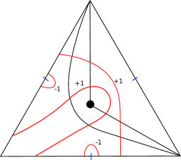
Figure 3: An example of a WKB triangulation of the once-punctured triangle and a lamination, corresponding to the line defect $B_{2}$ in the $(A_{1},D_{3})$ Argyres-Douglas theory.

We fix an orientation of each component of the lamination. Then we divide each component of the lamination into arcs crossing triangles. To each arc we assign the matrix $L$ ($R$) if the arc turns left (right),

$$L=\begin{pmatrix}1&0\\ 1&1\end{pmatrix},\qquad R=\begin{pmatrix}1&1\\ 0&1\end{pmatrix}.$$ (67)

When the lamination crosses an internal edge $E_{i}$ we assign the matrix

$$M_{E}=\begin{pmatrix}\sqrt{{\mathcal{X}}_{E}}&0\\ 0&1/\sqrt{{\mathcal{X}}_{E}}\end{pmatrix}.$$ (68)

To the initial and final points of each component we assign the vectors

$$E^{R}=\begin{pmatrix}0&1\end{pmatrix},\quad E^{L}=\begin{pmatrix}1&0\end{pmatrix},\quad B^{R}=\begin{pmatrix}1\\ 0\end{pmatrix},\quad B^{L}=\begin{pmatrix}0\\ 1\end{pmatrix},$$ (69)

choosing $L$ or $R$ according to whether the endpoint is on the left or the right of the marked point of the boundary edge. Then we multiply these matrices in order, with the beginning of the path corresponding to the rightmost matrix, to get a number for each component. If the component has weight $k$ we raise this number to the $k$-th power. Finally we multiply the contributions from all components to get the vev.

In the example of Figure 3 above, the contribution from the left long component with weight $+1$ is

$$E^{R}LM_{E_{2}}LM_{E_{3}}RM_{E_{1}}LM_{E_{2}}LB^{R}=\\ \frac{1}{\sqrt{{\mathcal{X}}_{1}{\mathcal{X}}_{3}}}+\frac{1}{\sqrt{{\mathcal{X}}_{1}{\mathcal{X}}_{3}}{\mathcal{X}}_{2}}+2\frac{\sqrt{{\mathcal{X}}_{3}}}{\sqrt{{\mathcal{X}}_{1}}}+\sqrt{{\mathcal{X}}_{1}{\mathcal{X}}_{3}}+\frac{\sqrt{{\mathcal{X}}_{3}}}{\sqrt{{\mathcal{X}}_{1}}{\mathcal{X}}_{2}}+\frac{{\mathcal{X}}_{2}\sqrt{{\mathcal{X}}_{3}}}{\sqrt{{\mathcal{X}}_{1}}}+{\mathcal{X}}_{2}\sqrt{{\mathcal{X}}_{1}{\mathcal{X}}_{3}}.$$ (70)

Similarly, the contribution from the right long component with weight $+1$ is $\sqrt{{\mathcal{X}}_{3}/{\mathcal{X}}_{1}}$. The short components with weight $-1$ contribute 1. The total contribution from this lamination is

$$\frac{1}{{\mathcal{X}}_{1}}+\frac{1}{{\mathcal{X}}_{1}{\mathcal{X}}_{2}}+{\mathcal{X}}_{3}+2\frac{{\mathcal{X}}_{3}}{{\mathcal{X}}_{1}}+\frac{{\mathcal{X}}_{3}}{{\mathcal{X}}_{1}{\mathcal{X}}_{2}}+{\mathcal{X}}_{2}{\mathcal{X}}_{3}+\frac{{\mathcal{X}}_{2}{\mathcal{X}}_{3}}{{\mathcal{X}}_{1}}.$$ (71)

Thus (71) gives the generating function of framed BPS states associated to this line defect, without spin information.

4.5 Framed BPS indices in class ${\mathcal{S}}[A_{1}]$ theories, with spin

We continue with our example from §4.4. Incorporating the spin information requires us to take each term in (71) and assign it the correct power of $q$. The work of Galakhov:2014xba ; Gabella:2016zxu provides a rule for determining these powers. The first step is to associate the terms in (71) to arcs on a branched double cover $\Sigma$ of the disc following the “path lifting” rules of Gaiotto:2012rg , as follows.

The double cover $\Sigma$ is presented concretely: in each triangle we fix one branch point and three branch cuts, as in the left side of Figure 4; the double cover has sheets labeled $1$ and $2$, and at each cut sheet $1$ is glued to sheet $2$ and vice versa. Next, note that each term in (71) comes from products of two specific chains of matrix elements: e.g. the term $\frac{1}{{\mathcal{X}}_{1}}$ comes from product of two contributions. As an example, the first contribution comes from taking the $(2,2)$ entries of the matrices from the beginning to the second-to-last $L$, then taking the $(2,1)$ entry of that $L$, then the $(1,1)$ entries of all the rest. Each of these matrix elements corresponds to an arc on the double cover, which we regard as a “lift” of the corresponding arc of the lamination. In Figure 4 we show three arcs corresponding to the three nonzero matrix elements of each of $L$ and $R$; the arc for the $(i,j)$ matrix element begins on sheet $j$ and ends on sheet $i$.

Concatenating these arcs gives a long path $P$ on $\Sigma$, associated to the term in (71) which we are studying. If $P$ has no self-intersections then we assign this term the factor $q^{0}$. If there are self-intersections then each contributes a factor $q^{\frac{1}{2}}$ or $q^{-{\frac{1}{2}}}$, according to Figure 6, where the arc which appears later in the path is drawn higher.

To illustrate how this works, we consider the term

$$2\frac{{\mathcal{X}}_{3}}{{\mathcal{X}}_{1}}$$ (72)

in (71). The factor $2$ here means (72) is a sum of two contributions, associated to two different lifted paths: we show one of them in Figure 5. There is one crossing in Figure 5, where both strands are lifted to sheet $1$. Comparing this crossing to Figure 6, we see that this term should be weighted by $q^{{\frac{1}{2}}}$. Drawing a similar picture for the other contribution to (72) we see that it gets weighted by $q^{-{\frac{1}{2}}}$. Thus altogether (72) is replaced by

$$(q^{\frac{1}{2}}+q^{-{\frac{1}{2}}})\frac{{\mathcal{X}}_{3}}{{\mathcal{X}}_{1}},$$ (73)

which tells us that the $2$ framed BPS states with charge $\gamma_{3}-\gamma_{1}$ come in a $2$-dimensional multiplet of the rotation group $SO(3)$. Carrying out similar computations for the other terms one finds (as expected) that all of them come with the factor $q^{0}$, i.e. they are in the trivial representation of $SO(3)$. Thus altogether the $q$-deformed version of the generating function (71) turns out to be

$$\frac{1}{{\mathcal{X}}_{1}}+\frac{1}{{\mathcal{X}}_{1}{\mathcal{X}}_{2}}+{\mathcal{X}}_{3}+(q^{\frac{1}{2}}+q^{-{\frac{1}{2}}})\frac{{\mathcal{X}}_{3}}{{\mathcal{X}}_{1}}+\frac{{\mathcal{X}}_{3}}{{\mathcal{X}}_{1}{\mathcal{X}}_{2}}+{\mathcal{X}}_{2}{\mathcal{X}}_{3}+\frac{{\mathcal{X}}_{2}{\mathcal{X}}_{3}}{{\mathcal{X}}_{1}}.$$ (74)

This is exactly the generating function for the line defect generator $B_{2}$ in §6.1 below.

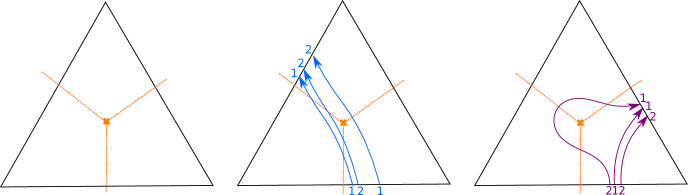
Figure 4: Left: a triangle with branch point and branch cuts marked. Middle: lifted left-turn paths. Right: lifted right-turn paths.

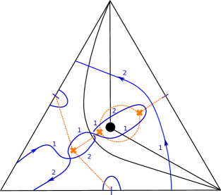
Figure 5: One of the lifted paths contributing to the term (72).

Figure 6: Rules for assigning powers of $q$ to self-crossings of the lifted path.

5 $(A_{1},A_{2N})$ Argyres-Douglas theories

In this section we present the results of explicit computations verifying the commutativity (16) in the Argyres-Douglas theories of type $(A_{1},A_{2})$, $(A_{1},A_{4})$ and $(A_{1},A_{6})$.

5.1 $(A_{1},A_{2})$ Argyres-Douglas theory

Figure 7: A BPS quiver for ($A_{1},A_{2}$) Argyres-Douglas theory.

We consider $(A_{1},A_{2})$ Argyres-Douglas theory and choose the chamber represented by the BPS quiver in Figure 7 containing two BPS particles: (in increasing central charge phase order)

$$\gamma_{1},\gamma_{2}.$$ (75)

There are five non-identity line defect generators. Assuming the line defect phase is smaller than the phases of all BPS particles, the generating functions are Cordova:2013bza ; Gaiotto:2010be :

$$\begin{split}F(L_{1})&=X_{\gamma_{1}},\\ F(L_{2})&=X_{\gamma_{2}}+X_{\gamma_{1}+\gamma_{2}},\\ F(L_{3})&=X_{-\gamma_{1}}+X_{-\gamma_{1}+\gamma_{2}}+X_{\gamma_{2}},\\ F(L_{4})&=X_{-\gamma_{1}-\gamma_{2}}+X_{-\gamma_{1}},\\ F(L_{5})&=X_{-\gamma_{2}}.\end{split}$$ (76)

In the geometric picture these generators $L_{i}$ correspond to five laminations which are rotated into each other under the monodromy action. As a result their generating functions are related to each other by the action of powers of the monodromy operator.

The Schur index with $L_{i}$ inserted is computed via Cordova:2016uwk :

$${\mathcal{I}}_{L_{i}}(q)=(q)_{\infty}^{2}\text{Tr}[F(L_{i})S(q)\overline{S}(q)],\quad S(q)=E_{q}(X_{\gamma_{1}})E_{q}(X_{\gamma_{2}}).$$ (77)

The corresponding $2d$ chiral algebra is the $(2,5)$ minimal model Cordova:2015nma ; Beem:2013sza ; Beem:2014zpa , which has two primaries: the vacuum $\Phi_{1,1}$ and $\Phi_{1,2}$ with weight $-1/5$. In general, characters of $\Phi_{s,r}$ in the $(p,p^{\prime})$ minimal model ($1\leq s\leq p-1$, $1\leq r\leq p^{\prime}-1$) are given by D.Francesco :

$$\begin{split}\chi_{s,r}(q)&=q^{-\frac{(rp-sp^{\prime})^{2}-(p-p^{\prime})^{2}}{4pp^{\prime}}+\frac{1}{24}(1-\frac{6(p-p^{\prime})^{2}}{pp^{\prime}})}\bigg{(}K_{s,r}^{p,p^{\prime}}(q)-K_{-s,r}^{p,p^{\prime}}(q)\bigg{)},\\ K_{s,r}^{p,p^{\prime}}(q)&=\frac{1}{q^{\frac{1}{24}}(q)_{\infty}}\displaystyle\sum\limits_{n\in\mathbb{Z}}q^{\frac{(2pp^{\prime}n+pr-p^{\prime}s)^{2}}{4pp^{\prime}}}.\end{split}$$ (78)

The line defect Schur index ${\mathcal{I}}_{L_{i}}(q)$ does not depend on the index $i$ and admits the following character expansion Cordova:2016uwk :

$${\mathcal{I}}_{L}(q)=q^{-\frac{1}{2}}\big{(}\chi_{1,1}(q)-\chi_{1,2}(q)\big{)}.$$ (79)

Similarly, the Schur index with two $L_{i}$ inserted is given by Cordova:2016uwk :

$${\mathcal{I}}_{L_{i}L_{j}}(q)=(q)_{\infty}^{2}\text{Tr}[F(L_{i})F(L_{j})S(q)\overline{S}(q)].$$ (80)

Unlike ${\mathcal{I}}_{L_{i}}(q)$, ${\mathcal{I}}_{L_{i}L_{j}}(q)$ does depend on $i$ and $j$, though this dependence disappears in the limit $q\to 1$. Expansions of ${\mathcal{I}}_{L_{i}L_{j}}(q)$ in terms of characters are given as follows:

$$\begin{split}{\mathcal{I}}_{L_{i}L_{i}}(q)={\mathcal{I}}_{L_{i}L_{i-1}}(q)&=(q^{-1}+q^{-2})\chi_{1,1}(q)-q^{-2}\chi_{1,2}(q),\\ {\mathcal{I}}_{L_{i}L_{i+1}}(q)={\mathcal{I}}_{L_{i}L_{i-2}}(q)&=(1+q^{-1})\chi_{1,1}(q)-q^{-1}\chi_{1,2}(q),\\ {\mathcal{I}}_{L_{i}L_{i+2}}(q)&=2\chi_{1,1}(q)-\chi_{1,2}(q).\end{split}$$ (81)

The map $f$ is given by

$$I\xrightarrow{f}[\Phi_{1,1}],\quad L_{i}\xrightarrow{f}[L]:=[\Phi_{1,1}]-[\Phi_{1,2}].$$ (82)

Moreover,

$$L_{i}L_{j}\xrightarrow{f}[LL]:=2[\Phi_{1,1}]-[\Phi_{1,2}].$$ (83)

Recall that the non-trivial fusion rule in $(2,5)$ minimal model is given by

$$[\Phi_{1,2}]\times[\Phi_{1,2}]=[\Phi_{1,1}]+[\Phi_{1,2}].$$ (84)

Combining with (82) and (83) we have

$$[LL]=[L]\times[L],$$ (85)

as first observed in Cordova:2016uwk .

Figure 8: The classical monodromy action in the $(A_{1},A_{2})$ theory, which rotates the triangulation of the pentagon clockwise by $2$ units, is equivalent to a single flip which replaces the $35$ edge by a $14$ edge.

Next we consider the fixed points of $U(1)_{r}$. For this purpose we found it convenient to use the geometric picture as described in §3.3. The classical monodromy action $M$ is directly given by a single flip: see Figure 8. According to (58) the concrete transformation is given by

$${\mathcal{X}}_{\gamma_{1}}\to\frac{1}{{\mathcal{X}}_{\gamma_{2}}},\quad{\mathcal{X}}_{\gamma_{2}}\to\frac{{\mathcal{X}}_{\gamma_{1}}{\mathcal{X}}_{\gamma_{2}}}{1+{\mathcal{X}}_{\gamma_{2}}}.$$ (86)

Thus the fixed locus is

$${\mathcal{X}}_{\gamma_{1}}^{2}-{\mathcal{X}}_{\gamma_{1}}-1=0,\quad{\mathcal{X}}_{\gamma_{2}}=\frac{1}{{\mathcal{X}}_{\gamma_{1}}}.$$ (87)

This locus consists of two points, which we label I, II. At these points the $X_{\gamma}$ evaluate to:

$$\text{I}:({\mathcal{X}}_{\gamma_{1}},{\mathcal{X}}_{\gamma_{2}})=\left(\frac{1-\sqrt{5}}{2},-\frac{1+\sqrt{5}}{2}\right),\quad\text{II}:({\mathcal{X}}_{\gamma_{1}},{\mathcal{X}}_{\gamma_{2}})=\left(\frac{1+\sqrt{5}}{2},-\frac{1-\sqrt{5}}{2}\right).$$ (88)

To construct the map $g:{\mathcal{L}}\to{\mathcal{O}}(F)$, for any line defect generator $L_{i}$ we evaluate $F({L_{i}})$ at these two fixed points, using (76). As expected, the dependence on $L_{i}$ disappears in the process:

$$L_{i}\xrightarrow{g}(F_{L_{i}}^{\text{I}},F_{L_{i}}^{\text{II}})=\left(\frac{1-\sqrt{5}}{2},\frac{1+\sqrt{5}}{2}\right).$$ (89)

Of course we also have the trivial line defect, whose vev is $1$ at every fixed point:

$$1\xrightarrow{g}(1,1).$$ (90)

Finally, we follow the recipe described in §1.4, §1.5 to construct the isomorphism $h:{\mathcal{V}}\to{\mathcal{O}}(F)$. We need the fusion matrices, which are given by

$$N_{\Phi_{1,1}}=\begin{pmatrix}1&0\\ 0&1\end{pmatrix},\qquad N_{\Phi_{1,2}}=\begin{pmatrix}0&1\\ 1&1\end{pmatrix}.$$ (91)

The modular $S$-matrix is D.Francesco :

$$S=\frac{2}{\sqrt{5}}\begin{pmatrix}-\sin\frac{2\pi}{5}&\sin\frac{4\pi}{5}\\ \sin\frac{4\pi}{5}&\sin\frac{2\pi}{5}\end{pmatrix}.$$ (92)

Thus the fusion matrices are diagonalized by the $S$ matrix,

$$\hat{N}_{\Phi_{1,1}}=SN_{\Phi_{1,1}}S^{-1}=\begin{pmatrix}1&0\\ 0&1\end{pmatrix},\qquad\hat{N}_{\Phi_{1,2}}=SN_{\Phi_{1,2}}S^{-1}=\begin{pmatrix}\frac{1-\sqrt{5}}{2}&0\\ 0&\frac{1+\sqrt{5}}{2}\end{pmatrix}.$$ (93)

As we explained in §1.4-§1.5, the map $h$ takes each of $\Phi_{1,1}$ and $\Phi_{1,2}$ to its eigenvalues. So, it takes $h(\Phi_{1,1})=(1,1)$ and either $h(\Phi_{1,2})=(\frac{1-\sqrt{5}}{2},\frac{1+\sqrt{5}}{2})$ or $h(\Phi_{1,2})=(\frac{1+\sqrt{5}}{2},\frac{1-\sqrt{5}}{2})$. To decide which is the right ordering, we need to know the dictionary between $U(1)_{r}$ fixed points and eigenspaces of the fusion operators. These eigenspaces themselves correspond to primary fields, so equivalently, we need the dictionary between the fixed points I, II and the primary fields $\Phi_{1,1}$, $\Phi_{1,2}$. This dictionary is determined by the table below:

fixed point	weights of $M$	weights of $U(1)_{r}$	primary field
I	${\mathrm{e}}^{2\pi{\mathrm{i}}(3/5)},{\mathrm{e}}^{2\pi{\mathrm{i}}(2/5)}$	$\frac{3}{5},\frac{2}{5}$	$\Phi_{1,2}$
II	${\mathrm{e}}^{2\pi{\mathrm{i}}(6/5)},{\mathrm{e}}^{-2\pi{\mathrm{i}}(1/5)}$	$\frac{6}{5},-\frac{1}{5}$	$\Phi_{1,1}$

In this table, to determine the weights of $M$ at each fixed point, we computed directly the linearization of the classical monodromy (86). On the other side, the dictionary between primary fields and $U(1)$ weights is taken from Fredrickson:2017yka . At any rate, we can now read off that $\Phi_{1,1}$ corresponds to fixed point II and $\Phi_{1,2}$ corresponds to fixed point I. Combining this with (93), $h$ is given by:

$$[\Phi_{1,1}]\xrightarrow{h}(1,1),\quad[\Phi_{1,2}]\xrightarrow{h}\Big{(}\frac{1+\sqrt{5}}{2},\frac{1-\sqrt{5}}{2}\Big{)}.$$ (94)

Composing this with $f$ from (82) we have

$$L_{i}\xrightarrow{h\circ f}\Big{(}\frac{1-\sqrt{5}}{2},\frac{1+\sqrt{5}}{2}\Big{)}.$$ (95)

Comparing this with (89) we see that the diagram indeed commutes.

5.2 An intermission on the homomorphism property

To make sure $f$ is a homomorphism, (85) needs to hold not only for the generators $L_{i}$ but also for arbitrary line defects. This would involve checking e.g.

$$[LLL]\stackrel{{\scriptstyle?}}{{=}}[L]\times[L]\times[L]$$ (96)

and similar relations for higher number of line defect generators. As an example let us consider the case of three line defect generators. The line defect Schur index is given by

$${\mathcal{I}}_{L_{i}L_{j}L_{k}}(q)=(q)^{2}_{\infty}\text{Tr}[F(L_{i})F(L_{j})F(L_{k})S(q)\overline{S}(q)].$$ (97)

There are many relations between ${\mathcal{I}}_{L_{i}L_{j}L_{k}}$,

$${\mathcal{I}}_{L_{i-1}L_{i}L_{i+2}}={\mathcal{I}}_{L_{i-1}L_{i}L_{i+1}}={\mathcal{I}}_{L_{i-2}L_{i}L_{i+1}},$$

$${\mathcal{I}}_{L_{i}L_{i}L_{i+2}}={\mathcal{I}}_{L_{i-2}L_{i}L_{i+2}}={\mathcal{I}}_{L_{i-2}L_{i}L_{i}},$$

$${\mathcal{I}}_{L_{i+2}L_{i}L_{i+1}}={\mathcal{I}}_{L_{i}L_{i}L_{i+1}}={\mathcal{I}}_{L_{i+2}L_{i}L_{i}}={\mathcal{I}}_{L_{i-1}L_{i}L_{i}}={\mathcal{I}}_{L_{i}L_{i}L_{i-2}}={\mathcal{I}}_{L_{i-1}L_{i}L_{i-2}},$$

$${\mathcal{I}}_{L_{i+1}L_{i}L_{i}}={\mathcal{I}}_{L_{i}L_{i}L_{i}}={\mathcal{I}}_{L_{i}L_{i}L_{i-1}}=q^{-2}{\mathcal{I}}_{L_{i-1}L_{i}L_{i-2}},$$

$${\mathcal{I}}_{L_{i+1}L_{i}L_{i+1}}={\mathcal{I}}_{L_{i-1}L_{i}L_{i-1}}={\mathcal{I}}_{L_{i+1}L_{i}L_{i-1}}=q^{-1}{\mathcal{I}}_{L_{i-1}L_{i}L_{i-2}},$$

$${\mathcal{I}}_{L_{i+2}L_{i}L_{i+2}}={\mathcal{I}}_{L_{i+1}L_{i}L_{i+2}}={\mathcal{I}}_{L_{i+2}L_{i}L_{i-1}}={\mathcal{I}}_{L_{i-2}L_{i}L_{i-1}}={\mathcal{I}}_{L_{i+1}L_{i}L_{i-2}}={\mathcal{I}}_{L_{i-2}L_{i}L_{i-2}}.$$

The independent indices admit the following character expansions,

$${\mathcal{I}}_{L_{i-2}L_{i}L_{i+1}} =q^{-\frac{1}{2}}\big{(}(1+2q)\chi_{1,1}(q)-(1+q)\chi_{1,2}(q)\big{)},$$

$${\mathcal{I}}_{L_{i-2}L_{i}L_{i}} =q^{-\frac{1}{2}}\big{(}(2+q)\chi_{1,1}(q)-2\chi_{1,2}(q)\big{)},$$

$${\mathcal{I}}_{L_{i-1}L_{i}L_{i-2}} =q^{-\frac{1}{2}}\big{(}(1+q^{-1}+q^{-2})\chi_{1,1}(q)-(1+q^{-2})\chi_{1,2}(q)\big{)},$$

$${\mathcal{I}}_{L_{i+2}L_{i}L_{i-2}} =q^{-\frac{1}{2}}\big{(}3\chi_{1,1}(q)-2\chi_{1,2}(q)\big{)},$$

$${\mathcal{I}}_{L_{i-2}L_{i}L_{i-2}} =q^{-\frac{1}{2}}\big{(}(2+q^{-1})\chi_{1,1}(q)-(1+q^{-1})\chi_{1,2}(q)\big{)}.$$

We immediately see that

$$L_{i}L_{j}L_{k}\xrightarrow{f}[LLL]:=3[\Phi_{1,1}]-2[\Phi_{1,2}]=[L]\times[L]\times[L].$$ (98)

In principal, to prove that $f$ is a homomorphism we need to repeat the above calculation for arbitrary number of line defect generator insertions. We are not able to prove it in this paper. Instead we offer some arguments about why we believe $f$ is indeed a homomorphism. We have seen explicitly that the images of $L_{i}L_{j}$ and $L_{i}L_{j}L_{k}$ under $f$ does not depend on the index $i$. In other examples that we consider in this paper we also checked the image of $L_{\rho i}L_{\mu j}$ does not depend on $i$. Although we don’t have a proof for now, we conjecture this phenomenon is general, i.e. the image of $L_{\rho_{1}i_{1}}L_{\rho_{2}i_{2}}\dots L_{\rho_{n}i_{n}}$ under $f$ does not depend on $i_{1},\dots,i_{n}$. Combining this conjecture with relations between line defect generating functions one could see that $f$ is indeed a homomorphism.

We revisit the situation of three line defect generators. To compute the image of $L_{i}L_{j}L_{k}$ under $f$ we could pick any three line defect generators. Let’s recall the following relation between $F(L_{i})$ Gaiotto:2010be ; Cordova:2013bza :

$$F(L_{i})F(L_{i+2})=1+q^{\frac{1}{2}}F(L_{i+1}),$$ (99)

from which follows $[L]\times[L]=[\Phi_{1,1}]+[L]$. Schur index with insertion of $L_{i},L_{i+2},L_{k}$ is then given by

$${\mathcal{I}}_{L_{i}L_{i+2}L_{k}}(q)={\mathcal{I}}_{L_{k}}(q)+q^{\frac{1}{2}}{\mathcal{I}}_{L_{i+1}L_{k}}(q),$$ (100)

from which it follows that

$$[LLL]=[L]+[LL]=[L]\times[L]\times[L].$$ (101)

Similarly one could consider insertion of more line defect generators. By the conjecture, to compute the image of $L_{i_{1}}\dots L_{i_{n}}$ under $f$, it doesn’t matter what $i_{1},\dots,i_{n}$ are. Then we could again use (99) to reduce the number of line defect generators. Moreover this process is consistent with the fusion rules such that

$$[L\dots L]=[L]\times\dots\times[L].$$ (102)

For other Argyres-Douglas theories that we are considering in this paper, there are always enough relations between $F(L_{\alpha i})$ such that the same argument goes through provided our conjecture would hold.

5.3 $(A_{1},A_{4})$ Argyres-Douglas theory

We consider the $(A_{1},A_{4})$ Argyres-Douglas theory. We choose a chamber represented by the BPS quiver shown in Figure 9. Moreover our choice is made such that there are four BPS particles in this chamber. Their charges are (in increasing central charge phase order):

$$\gamma_{1},\gamma_{3},\gamma_{2},\gamma_{4}$$ (103)

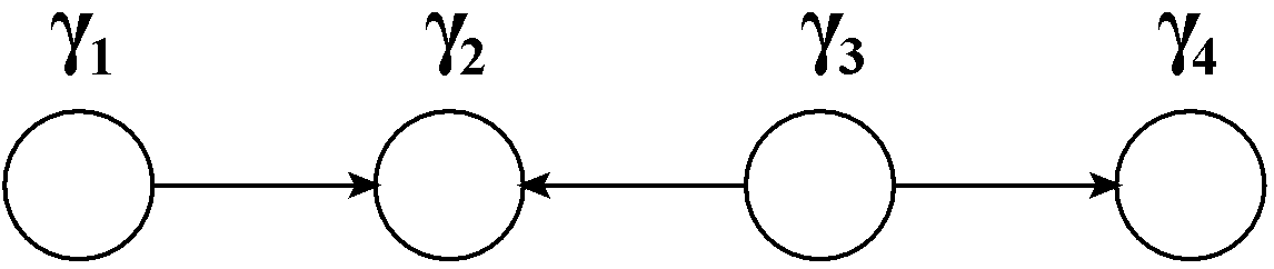
Figure 9: A BPS quiver for ($A_{1},A_{4}$) Argyres-Douglas theory.

Line defect generators in $(A_{1},A_{4})$ Argyres-Douglas theory and their generating functions were computed in Cordova:2016uwk . For completeness we reproduce their results here. Starting from the initial seed, we apply all possible left mutations to generate other seeds. There are in total $42$ seeds. Correspondingly there are $42$ dual cones. Each dual cone is bounded by four half-hyperplanes. Moreover, every three out of the four half-hyperplanes intersect at a half line. In total there are four such half-lines for each dual cone and they form edges of the dual cone. Each edge corresponds to the core charge of one line defect generator. For example, the dual cone for the initial seed is given by:

$$\check{\mathcal{C}}_{\{\gamma_{1},\gamma_{2},\gamma_{3},\gamma_{4}\}}=\bigg{\{}\displaystyle\sum\limits_{i=1}^{4}a_{i}\gamma_{i}\mid a_{2}\leq 0,a_{1}+a_{3}\geq 0,a_{2}+a_{4}\leq 0,a_{3}\geq 0\bigg{\}}.$$ (104)

Then we get four line defect generators whose core charges are given by

$$\gamma_{1},-\gamma_{1}+\gamma_{3},-\gamma_{2}+\gamma_{4},-\gamma_{4}.$$ (105)

Repeating this procedure for all $42$ dual cones we get $14$ edges. Thus the line defects in $(A_{1},A_{4})$ Argyres-Douglas theory are generated by the identity operator and $14$ nontrivial generators. Recall that the $(2,7)$ minimal model has two non-vacuum modules; therefore we have an expected multiplicity of $7$. In the class ${\mathcal{S}}$ realization of the theory this would correspond to the $\mathbb{Z}_{7}$ symmetry of the $7$-gon.

We assume that the line defect phase is smaller than the phases of all vanilla BPS particles, and calculate the generating function using consecutive right mutations on the framed quiver. For example, the line defect generator with core charge $\gamma_{c}=\gamma_{1}-\gamma_{3}$ goes through the following mutation sequence:

$$\begin{split}&\{\gamma_{1},\gamma_{2},\gamma_{3},\gamma_{4},\gamma_{c}\}\xrightarrow{\mu^{R}_{\gamma_{c}}}\{\gamma_{1},\gamma_{2},\gamma_{3},\gamma_{4}+\gamma_{c},-\gamma_{c}\}\xrightarrow{\mu^{R}_{\gamma_{4}+\gamma_{c}}}\\ &\{\gamma_{1},\gamma_{2},\gamma_{3}+\gamma_{4}+\gamma_{c},-\gamma_{4}-\gamma_{c},\gamma_{4}\}\xrightarrow{\mu^{R}_{\gamma_{3}+\gamma_{4}+\gamma_{c}}}\{\gamma_{1},\gamma_{2},-\gamma_{3}-\gamma_{4}-\gamma_{c},\gamma_{3},\gamma_{4}\},\end{split}$$ (106)

which implies that its generating function is

$$F(L)=X_{\gamma_{1}-\gamma_{3}}+X_{\gamma_{1}-\gamma_{3}+\gamma_{4}}+X_{\gamma_{1}+\gamma_{4}}.$$

The generating functions for all 14 line defect generators are (as given also in Cordova:2016uwk ):

$$F(A_{1}) =X_{-\gamma_{2}+\gamma_{4}},$$

$$F(A_{2}) =X_{-\gamma_{1}+\gamma_{3}},$$

$$F(A_{3}) =X_{\gamma_{2}-\gamma_{4}}+X_{\gamma_{1}+\gamma_{2}-\gamma_{4}},$$

$$F(A_{4}) =X_{\gamma_{1}-\gamma_{3}-\gamma_{4}}+X_{\gamma_{1}-\gamma_{3}},$$

$$F(A_{5}) =X_{-\gamma_{1}-\gamma_{4}}+X_{-\gamma_{1}+\gamma_{2}-\gamma_{4}}+X_{\gamma_{2}-\gamma_{4}},$$

$$F(A_{6}) =X_{-\gamma_{1}-\gamma_{2}+\gamma_{4}}+X_{-\gamma_{1}+\gamma_{4}}+X_{-\gamma_{1}+\gamma_{3}+\gamma_{4}},$$

$$F(A_{7}) =X_{\gamma_{1}-\gamma_{3}}+X_{\gamma_{1}-\gamma_{3}+\gamma_{4}}+X_{\gamma_{1}+\gamma_{4}},$$

$$F(B_{1}) =X_{\gamma_{1}},$$

$$F(B_{2}) =X_{-\gamma_{4}},$$

$$F(B_{3}) =X_{-\gamma_{1}-\gamma_{2}}+X_{-\gamma_{1}},$$

$$F(B_{4}) =X_{\gamma_{4}}+X_{\gamma_{3}+\gamma_{4}},$$

$$F(B_{5}) =X_{-\gamma_{1}}+X_{-\gamma_{1}+\gamma_{2}}+X_{\gamma_{2}}+X_{-\gamma_{1}+\gamma_{2}+\gamma_{3}}+X_{\gamma_{2}+\gamma_{3}},$$

$$F(B_{6}) =X_{-\gamma_{2}-\gamma_{3}}+X_{-\gamma_{3}}+X_{-\gamma_{2}-\gamma_{3}+\gamma_{4}}+X_{-\gamma_{3}+\gamma_{4}}+X_{\gamma_{4}},$$

$$F(B_{7}) =X_{-\gamma_{3}-\gamma_{4}}+X_{\gamma_{2}-\gamma_{3}-\gamma_{4}}+X_{\gamma_{1}+\gamma_{2}-\gamma_{3}-\gamma_{4}}+X_{-\gamma_{3}}+X_{\gamma_{2}-\gamma_{3}}+X_{\gamma_{1}+\gamma_{2}-\gamma_{3}}$$

$$\ \ +X_{\gamma_{2}}+X_{\gamma_{1}+\gamma_{2}}.$$

The generating functions for $A_{i}$ ($B_{i}$) are related to each other by the action of powers of the monodromy operator. The Schur index with line defect $A_{i}$ ($B_{i}$) inserted is computed using Cordova:2016uwk

$${\mathcal{I}}_{A_{i}}(q)=(q)_{\infty}^{4}\text{Tr}[F(A_{i})S(q)\overline{S}(q)],\quad{\mathcal{I}}_{B_{i}}(q)=(q)_{\infty}^{4}\text{Tr}[F(B_{i})S(q)\overline{S}(q)]$$ (107)

where in this particular chamber $S(q)$ is given by

$$S(q)=E_{q}(X_{\gamma_{1}})E_{q}(X_{\gamma_{3}})E_{q}(X_{\gamma_{2}})E_{q}(X_{\gamma_{4}}).$$ (108)

As described in Cordova:2016uwk , the Schur index with one line defect inserted does not depend on $i\in\{1,\dots,7\}$:

$$\begin{split}{\mathcal{I}}_{A}(q)&=q+q^{4}+q^{5}+q^{6}+2q^{7}+2q^{8}+3q^{9}+3q^{10}+\cdots,\\ {\mathcal{I}}_{B}(q)&=-q^{\frac{1}{2}}-q^{\frac{5}{2}}-q^{\frac{7}{2}}-q^{\frac{9}{2}}-2q^{\frac{11}{2}}-3q^{\frac{13}{2}}-3q^{\frac{15}{2}}-4q^{\frac{17}{2}}-5q^{\frac{19}{2}}+\cdots.\end{split}$$ (109)

The chiral algebra in this case is the $(2,7)$ Virasoro minimal model Cordova:2015nma ; Beem:2013sza ; Beem:2014zpa . There are three primary fields: the vacuum $\Phi_{1,1}$, $\Phi_{1,2}$ with weight $-2/7$ and $\Phi_{1,3}$ with weight $-3/7$. Line defect Schur indices admit the following expansions in terms of characters:

$$\begin{split}{\mathcal{I}}_{A}(q)&=q^{-1}\big{(}\chi_{1,3}(q)-\chi_{1,2}(q)\big{)},\\ {\mathcal{I}}_{B}(q)&=q^{-\frac{1}{2}}\big{(}\chi_{1,1}(q)-\chi_{1,2}(q)\big{)}.\end{split}$$ (110)

The map $f$ between the line defect algebra ${\mathcal{L}}$ and the Verlinde algebra ${\mathcal{V}}$ is then given by:

$$\begin{split}I&\xrightarrow{f}[\Phi_{1,1}],\\ A_{i}&\xrightarrow{f}[A]=[\Phi_{1,3}]-[\Phi_{1,2}],\\ B_{i}&\xrightarrow{f}[B]=[\Phi_{1,1}]-[\Phi_{1,2}].\end{split}$$ (111)

The non-trivial fusion rules in the $(2,7)$ Virasoro minimal model are:

$$\begin{split}[\Phi_{1,2}]\times[\Phi_{1,2}]&=[\Phi_{1,1}]+[\Phi_{1,3}],\\ [\Phi_{1,3}]\times[\Phi_{1,3}]&=[\Phi_{1,1}]+[\Phi_{1,2}]+[\Phi_{1,3}],\\ [\Phi_{1,2}]\times[\Phi_{1,3}]&=[\Phi_{1,2}]+[\Phi_{1,3}].\end{split}$$ (112)

As first checked in Cordova:2016uwk ,

$$\begin{split}[AA]&=[A]\times[A],\\ [BB]&=[B]\times[B],\\ [AB]&=[A]\times[B],\end{split}$$ (113)

which gives evidence $f$ is indeed a homomorphism ${\mathcal{L}}\to{\mathcal{V}}$.

Figure 10: The classical monodromy action in the $(A_{1},A_{4})$ theory is realized by a sequence of flips of triangulations of the $7$-gon. The initial triangulation differs from the final one by a clockwise rotation by $2$ units.

Now we turn to study the fixed points under the classical monodromy action $M$. By doing a series of flips (see Figure 10, the initial zigzag triangulation corresponds to the BPS quiver in Figure 9 using the dictionary in Gaiotto:2009hg . The monodromy action is given as follows:

$$\begin{split}{\mathcal{X}}_{\gamma_{1}}&\rightarrow\frac{1+{\mathcal{X}}_{\gamma_{2}}+{\mathcal{X}}_{\gamma_{4}}+{\mathcal{X}}_{\gamma_{2}}{\mathcal{X}}_{\gamma_{4}}+{\mathcal{X}}_{\gamma_{2}}{\mathcal{X}}_{\gamma_{3}}{\mathcal{X}}_{\gamma_{4}}}{{\mathcal{X}}_{\gamma_{2}}{\mathcal{X}}_{\gamma_{3}}},\\ {\mathcal{X}}_{\gamma_{2}}&\rightarrow\frac{{\mathcal{X}}_{\gamma_{1}}{\mathcal{X}}_{\gamma_{2}}{\mathcal{X}}_{\gamma_{3}}}{(1+{\mathcal{X}}_{\gamma_{2}}+{\mathcal{X}}_{\gamma_{2}}{\mathcal{X}}_{\gamma_{3}})[1+{\mathcal{X}}_{\gamma_{4}}+{\mathcal{X}}_{\gamma_{2}}(1+{\mathcal{X}}_{\gamma_{1}})(1+{\mathcal{X}}_{\gamma_{4}}+{\mathcal{X}}_{\gamma_{3}}{\mathcal{X}}_{\gamma_{4}})]},\\ {\mathcal{X}}_{\gamma_{3}}&\rightarrow\frac{(1+{\mathcal{X}}_{\gamma_{2}}+{\mathcal{X}}_{\gamma_{1}}{\mathcal{X}}_{\gamma_{2}})[1+{\mathcal{X}}_{\gamma_{4}}+{\mathcal{X}}_{\gamma_{2}}(1+{\mathcal{X}}_{\gamma_{4}}+{\mathcal{X}}_{\gamma_{3}}{\mathcal{X}}_{\gamma_{4}})]}{{\mathcal{X}}_{\gamma_{1}}{\mathcal{X}}_{\gamma_{2}}{\mathcal{X}}_{\gamma_{3}}{\mathcal{X}}_{\gamma_{4}}},\\ {\mathcal{X}}_{\gamma_{4}}&\rightarrow\frac{{\mathcal{X}}_{\gamma_{3}}{\mathcal{X}}_{\gamma_{4}}}{1+{\mathcal{X}}_{\gamma_{4}}+{\mathcal{X}}_{\gamma_{2}}(1+{\mathcal{X}}_{\gamma_{1}})(1+{\mathcal{X}}_{\gamma_{4}}+{\mathcal{X}}_{\gamma_{3}}{\mathcal{X}}_{\gamma_{4}})}.\end{split}$$ (114)

There are exactly three fixed points, which we label I, II, III. On the fixed points ${\mathcal{X}}_{\gamma}$ evaluate to

$$\begin{split}{\mathcal{X}}_{\gamma_{4}}&:(\alpha_{1},\alpha_{2},\alpha_{3}),\\ {\mathcal{X}}_{\gamma_{3}}&:(4+\alpha_{1}-2\alpha_{1}^{2},4+\alpha_{2}-2\alpha_{2}^{2},4+\alpha_{3}-2\alpha_{3}^{2}),\\ {\mathcal{X}}_{\gamma_{2}}&:(\alpha_{1}-\alpha_{1}^{2},\alpha_{2}-\alpha_{2}^{2},\alpha_{3}-\alpha_{3}^{2}),\\ {\mathcal{X}}_{\gamma_{1}}&:(2+\alpha_{1}-\alpha_{1}^{2},2+\alpha_{2}-\alpha_{2}^{2},2+\alpha_{3}-\alpha_{3}^{2}),\end{split}$$ (115)

where $\alpha_{i}$ are the three roots of the cubic equation

$$\alpha^{3}-\alpha^{2}-2\alpha+1=0.$$ (116)

Concretely,

$$\alpha_{1} =\frac{1}{3}\big{(}1-\frac{7}{a}(-1)^{1/3}+a(-1)^{2/3}\big{)},\quad\alpha_{2}=\frac{1}{3}\big{(}1+\frac{7}{a}(-1)^{2/3}-a(-1)^{1/3}\big{)},$$

$$\alpha_{3} =\frac{1}{3}\big{(}1+\frac{7}{a}+a\big{)},\quad\text{with}\quad a=\bigg{(}\frac{7}{2}\bigg{)}^{\frac{1}{3}}\big{(}-1+{\mathrm{i}}3\sqrt{3}\big{)}^{\frac{1}{3}}.$$

Evaluating the $F({A_{i}})$ at the fixed points we find that the values are independent of $i=1,\dots,7$, and similarly for $F({B_{i}})$, as expected. Concretely, we get

$$\begin{split}A_{i}&\xrightarrow{g}\bigg{(}\frac{1}{1-\alpha_{1}},\frac{1}{1-\alpha_{2}},\frac{1}{1-\alpha_{3}}\bigg{)},\\ B_{i}&\xrightarrow{g}\bigg{(}\frac{1}{\alpha_{1}},\frac{1}{\alpha_{2}},\frac{1}{\alpha_{3}}\bigg{)}.\end{split}$$ (117)

Finally we want to construct $h$. We have the following Verlinde matrices for $[\Phi_{1,2}]$ and $[\Phi_{1,3}]$:

$$N_{\Phi_{1,2}}=\begin{pmatrix}0&1&0\\ 1&0&1\\ 0&1&1\end{pmatrix},\quad N_{\Phi_{1,3}}=\begin{pmatrix}0&0&1\\ 0&1&1\\ 1&1&1\end{pmatrix}.$$ (118)

As before, we obtain $h$ by simultaneously diagonalizing $N_{\Phi_{1,2}}$ and $N_{\Phi_{1,3}}$ using $S$-matrix and then comparing with the correspondence between $U(1)$ fixed points and primaries of $(2,7)$ Virasoro minimal model. The $S$-matrix for the (2,7) minimal models is D.Francesco :

$$S=\frac{2}{\sqrt{7}}\begin{pmatrix}\text{cos}\frac{3\pi}{14}&-\text{cos}\frac{\pi}{14}&\text{sin}\frac{\pi}{7}\\ -\text{cos}\frac{\pi}{14}&-\text{sin}\frac{\pi}{7}&\text{cos}\frac{3\pi}{14}\\ \text{sin}\frac{\pi}{7}&\text{cos}\frac{3\pi}{14}&\text{cos}\frac{\pi}{14}\\ \end{pmatrix}.$$ (119)

$N_{\Phi_{1,2}}$ and $N_{\Phi_{1,3}}$ are simultaneously diagonalized by $S$:

$$SN_{\Phi_{1,2}}S^{-1}=\begin{pmatrix}\alpha_{1}&0&0\\ 0&\alpha_{2}&0\\ 0&0&\alpha_{3}\end{pmatrix},\quad SN_{\Phi_{1,3}}S^{-1}=\begin{pmatrix}\beta_{1}&0&0\\ 0&\beta_{2}&0\\ 0&0&\beta_{3}\end{pmatrix},$$ (120)

where

$$\beta_{1} =\frac{1}{3}\big{(}2+\frac{7}{b}(-1)^{2/3}-b(-1)^{1/3}\big{)},\quad\beta_{2}=\frac{1}{3}\big{(}2-\frac{7}{b}(-1)^{1/3}+b(-1)^{2/3}\big{)}$$

$$\beta_{3} =\frac{1}{3}\big{(}2+\frac{7}{b}+b\big{)},\quad\text{with}\quad b=\bigg{(}\frac{7}{2}\bigg{)}^{\frac{1}{3}}\big{(}1+{\mathrm{i}}3\sqrt{3}\big{)}^{\frac{1}{3}}.$$

According to Fredrickson-Neitzke ; Fredrickson:2017yka , the corresponding wild Hitchin moduli space has exactly three $U(1)_{r}$-fixed points, each of which corresponds to a primary field in the $(2,7)$ minimal model:

fixed point	weights of $M$	$U(1)_{r}$ weights	primary field
I	${\mathrm{e}}^{2\pi{\mathrm{i}}(3/7)},{\mathrm{e}}^{2\pi{\mathrm{i}}(4/7)},{\mathrm{e}}^{2\pi{\mathrm{i}}(5/7)},{\mathrm{e}}^{2\pi{\mathrm{i}}(2/7)}$	$\frac{3}{7},\frac{4}{7},\frac{5}{7},\frac{2}{7}$	$\Phi_{1,3}$
II	${\mathrm{e}}^{2\pi{\mathrm{i}}(8/7)},{\mathrm{e}}^{-2\pi{\mathrm{i}}(1/7)},{\mathrm{e}}^{2\pi{\mathrm{i}}(10/7)},{\mathrm{e}}^{-2\pi{\mathrm{i}}(3/7)}$	$\frac{8}{7},-\frac{1}{7},\frac{10}{7},-\frac{3}{7}$	$\Phi_{1,1}$
III	${\mathrm{e}}^{2\pi{\mathrm{i}}(8/7)},{\mathrm{e}}^{-2\pi{\mathrm{i}}(1/7)},{\mathrm{e}}^{2\pi{\mathrm{i}}(5/7)},{\mathrm{e}}^{2\pi{\mathrm{i}}(2/7)}$	$\frac{8}{7},-\frac{1}{7},\frac{5}{7},\frac{2}{7}$	$\Phi_{1,2}$

Using this table and (120), the isomorphism $h$ between ${\mathcal{V}}$ and ${\mathcal{O}}(F)$ is:

$$\begin{split}&[\Phi_{1,1}]\xrightarrow{h}(1,1,1),\\ &[\Phi_{1,2}]\xrightarrow{h}(\alpha_{3},\alpha_{1},\alpha_{2}),\\ &[\Phi_{1,3}]\xrightarrow{h}(\beta_{3},\beta_{1},\beta_{2}).\end{split}$$ (121)

The image of $A_{i}$ and $B_{i}$ under $h\circ f$ is then:

$$\begin{split}&A_{i}\xrightarrow{h\circ f}(\beta_{3}-\alpha_{3},\beta_{1}-\alpha_{1},\beta_{2}-\alpha_{2}),\\ &B_{i}\xrightarrow{h\circ f}(1-\alpha_{3},1-\alpha_{1},1-\alpha_{2}).\end{split}$$ (122)

Although it is not obvious, one can check that this indeed agrees with (117), so the diagram commutes, as desired.

5.4 $(A_{1},A_{6})$ Argyres-Douglas theory

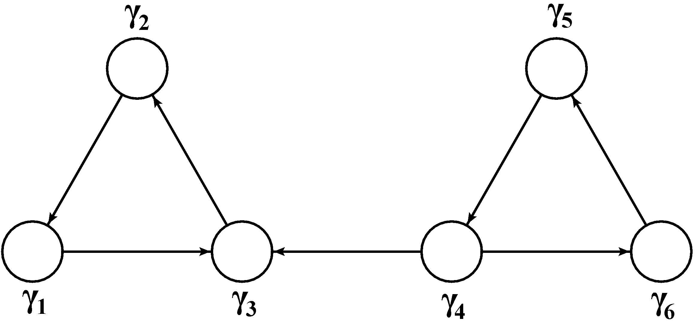
Figure 11: A BPS quiver for ($A_{1},A_{6}$) Argyres-Douglas theory.

Here we consider the $(A_{1},A_{6})$ Argyres-Douglas theory. This theory has a new feature: at one of the fixed points (fixed point I below), some of the cluster coordinates ${\mathcal{X}}_{\gamma}$ associated to the canonical chamber blow up. This being so, computing the fixed points of the classical monodromy in that chamber actually misses one fixed point. Thus, with the benefit of hindsight, we choose a different chamber, whose BPS quiver is shown in Figure 11.

There are eight BPS particles in this chamber, with the following charges (in increasing central charge phase order):

$$\gamma_{4},\gamma_{6},\gamma_{4}+\gamma_{5},\gamma_{5},\gamma_{3},\gamma_{1}+\gamma_{3},\gamma_{2},\gamma_{1}.$$ (123)

Quiver mutation starting from this chamber generates in total 429 seeds. After mutating back to the original seed the 429 dual cones span the whole charge lattice. Each dual cone is bounded by six half-hyperplanes. Every five of the six half-hyperplanes intersect at a half line which forms an edge of the dual cone and there are six edges for each dual cone. For example, the six edges of the dual cone for the initial seed $\check{C}_{\{\gamma_{1},\gamma_{2},\gamma_{3},\gamma_{4},\gamma_{5},\gamma_{6}\}}$ are spanned by:

$$\begin{split}&\gamma_{2}+\gamma_{4}+\gamma_{5}+\gamma_{6},-\gamma_{1}+\gamma_{4}+\gamma_{5}+\gamma_{6},\gamma_{4}+\gamma_{5}+\gamma_{6},\\ &-\gamma_{1}-\gamma_{2}-\gamma_{3},-\gamma_{1}-\gamma_{2}-\gamma_{3}+\gamma_{6},-\gamma_{1}-\gamma_{2}-\gamma_{3}-\gamma_{5}.\end{split}$$ (124)

Repeating this for all $429$ dual cones we get in total $27$ edges. Correspondingly there are $27$ nontrivial line defect generators in the $(A_{1},A_{6})$ theory. The $(2,9)$ minimal model has three non-vacuum modules, so there is a multiplicity of $9$, corresponding to the $\mathbb{Z}_{9}$ symmetry of the $9$-gon. Assuming that the line defect phase is smaller than central charge phases of all vanilla BPS particles, their generating functions are:

$$F(A_{1}) =X_{\gamma_{1}+\gamma_{2}+\gamma_{3}-\gamma_{6}}+X_{\gamma_{1}+\gamma_{2}+\gamma_{3}+\gamma_{5}-\gamma_{6}}+X_{\gamma_{1}+\gamma_{2}+\gamma_{3}+\gamma_{5}},$$

$$F(A_{2}) =X_{-\gamma_{2}-\gamma_{4}-\gamma_{5}-\gamma_{6}}+X_{\gamma_{1}-\gamma_{2}-\gamma_{4}-\gamma_{5}-\gamma_{6}}+X_{\gamma_{1}-\gamma_{4}-\gamma_{5}-\gamma_{6}},$$

$$F(A_{3}) =X_{-\gamma_{1}-\gamma_{2}-\gamma_{3}-\gamma_{5}},$$

$$F(A_{4}) =X_{\gamma_{2}+\gamma_{4}+\gamma_{5}+\gamma_{6}},$$

$$F(A_{5}) =X_{-\gamma_{1}-\gamma_{2}-\gamma_{3}+\gamma_{6}},$$

$$F(A_{6}) =X_{\gamma_{1}+\gamma_{2}+\gamma_{3}+\gamma_{5}}+X_{\gamma_{1}+\gamma_{2}+\gamma_{3}+\gamma_{5}+\gamma_{6}}+X_{\gamma_{1}+\gamma_{2}+\gamma_{3}+\gamma_{4}+\gamma_{5}+\gamma_{6}},$$

$$F(A_{7}) =X_{\gamma_{1}-\gamma_{4}-\gamma_{5}-\gamma_{6}}+X_{\gamma_{1}+\gamma_{2}-\gamma_{4}-\gamma_{5}-\gamma_{6}}+X_{\gamma_{1}+\gamma_{2}+\gamma_{3}-\gamma_{4}-\gamma_{5}-\gamma_{6}}+X_{\gamma_{1}+\gamma_{2}+\gamma_{3}-\gamma_{5}-\gamma_{6}}$$

$$\ \ +X_{\gamma_{1}+\gamma_{2}+\gamma_{3}-\gamma_{6}},$$

$$F(A_{8}) =X_{-\gamma_{1}-\gamma_{2}-\gamma_{3}-\gamma_{4}-\gamma_{5}-\gamma_{6}}+X_{-\gamma_{1}-\gamma_{2}-\gamma_{4}-\gamma_{5}-\gamma_{6}}+X_{-\gamma_{2}-\gamma_{4}-\gamma_{5}-\gamma_{6}},$$

$$F(A_{9}) =X_{-\gamma_{1}+\gamma_{4}+\gamma_{5}+\gamma_{6}},$$

$$F(B_{1}) =X_{-\gamma_{5}-\gamma_{6}}+X_{-\gamma_{6}},$$

$$F(B_{2}) =X_{\gamma_{1}}+X_{\gamma_{1}+\gamma_{2}},$$

$$F(B_{3}) =X_{\gamma_{5}}+X_{\gamma_{5}+\gamma_{6}},$$

$$F(B_{4}) =X_{-\gamma_{1}-\gamma_{2}}+X_{-\gamma_{2}},$$

$$F(B_{5}) =X_{\gamma_{6}}+X_{\gamma_{4}+\gamma_{6}},$$

$$F(B_{6}) =X_{-\gamma_{1}-\gamma_{3}}+X_{-\gamma_{1}},$$

$$F(B_{7}) =X_{-\gamma_{2}-\gamma_{3}-\gamma_{4}-\gamma_{5}}+X_{-\gamma_{3}-\gamma_{4}-\gamma_{5}}+X_{-\gamma_{4}-\gamma_{5}}+X_{-\gamma_{5}},$$

$$F(B_{8}) =X_{-\gamma_{4}-\gamma_{6}}+X_{-\gamma_{4}}+X_{\gamma_{3}-\gamma_{4}-\gamma_{6}}+X_{\gamma_{3}-\gamma_{4}}+X_{\gamma_{3}}+X_{\gamma_{1}+\gamma_{3}-\gamma_{4}-\gamma_{6}}+X_{\gamma_{1}+\gamma_{3}-\gamma_{4}}+X_{\gamma_{1}+\gamma_{3}},$$

$$F(B_{9}) =X_{\gamma_{2}}+X_{\gamma_{2}+\gamma_{3}}+X_{\gamma_{2}+\gamma_{3}+\gamma_{4}}+X_{\gamma_{2}+\gamma_{3}+\gamma_{4}+\gamma_{5}},$$

$$F(C_{1}) =X_{-\gamma_{1}-\gamma_{2}-\gamma_{3}},$$

$$F(C_{2}) =X_{\gamma_{4}+\gamma_{5}+\gamma_{6}},$$

$$F(C_{3}) =X_{\gamma_{1}+\gamma_{2}+\gamma_{3}}+X_{\gamma_{1}+\gamma_{2}+\gamma_{3}+\gamma_{4}}+X_{\gamma_{1}+\gamma_{2}+\gamma_{3}+\gamma_{4}+\gamma_{5}},$$

$$F(C_{4}) =X_{-\gamma_{2}-\gamma_{3}-\gamma_{4}-\gamma_{5}-\gamma_{6}}+X_{-\gamma_{3}-\gamma_{4}-\gamma_{5}-\gamma_{6}}+X_{-\gamma_{4}-\gamma_{5}-\gamma_{6}},$$

$$F(C_{5}) =X_{\gamma_{1}-\gamma_{4}-\gamma_{6}}+X_{\gamma_{1}-\gamma_{4}}+X_{\gamma_{1}+\gamma_{2}-\gamma_{4}-\gamma_{6}}+X_{\gamma_{1}+\gamma_{2}-\gamma_{4}}+X_{\gamma_{1}+\gamma_{2}+\gamma_{3}-\gamma_{4}-\gamma_{6}}$$

$$\ \ +X_{\gamma_{1}+\gamma_{2}+\gamma_{3}-\gamma_{4}}+X_{\gamma_{1}+\gamma_{2}+\gamma_{3}},$$

$$F(C_{6}) =X_{-\gamma_{4}-\gamma_{5}-\gamma_{6}}+X_{\gamma_{3}-\gamma_{4}-\gamma_{5}-\gamma_{6}}+X_{\gamma_{3}-\gamma_{5}-\gamma_{6}}+X_{\gamma_{3}-\gamma_{6}}+X_{\gamma_{1}+\gamma_{3}-\gamma_{4}-\gamma_{5}-\gamma_{6}}$$

$$\ \ +X_{\gamma_{1}+\gamma_{3}-\gamma_{5}-\gamma_{6}}+X_{\gamma_{1}+\gamma_{3}-\gamma_{6}},$$

$$F(C_{7}) =X_{-\gamma_{1}-\gamma_{2}-\gamma_{3}-\gamma_{4}-\gamma_{5}}+X_{-\gamma_{1}-\gamma_{2}-\gamma_{4}-\gamma_{5}}+X_{-\gamma_{1}-\gamma_{2}-\gamma_{5}}+X_{-\gamma_{2}-\gamma_{4}-\gamma_{5}}+X_{-\gamma_{2}-\gamma_{5}},$$

$$F(C_{8}) =X_{\gamma_{2}+\gamma_{5}}+X_{\gamma_{2}+\gamma_{5}+\gamma_{6}}+X_{\gamma_{2}+\gamma_{3}+\gamma_{5}}+X_{\gamma_{2}+\gamma_{3}+\gamma_{5}+\gamma_{6}}+X_{\gamma_{2}+\gamma_{3}+\gamma_{4}+\gamma_{5}+\gamma_{6}},$$

$$F(C_{9}) =X_{-\gamma_{1}-\gamma_{3}+\gamma_{6}}+X_{-\gamma_{1}+\gamma_{6}}+X_{-\gamma_{1}+\gamma_{4}+\gamma_{6}}.$$

In this chosen chamber the spectrum generator $S(q)$ is given by

$$S(q) =E_{q}(X_{\gamma_{4}})E_{q}(X_{\gamma_{6}})E_{q}(X_{\gamma_{4}+\gamma_{5}})E_{q}(X_{\gamma_{5}})E_{q}(X_{\gamma_{3}})E_{q}(X_{\gamma_{1}+\gamma_{3}})E_{q}(X_{\gamma_{2}})E_{q}(X_{\gamma_{1}})$$

$$=\displaystyle\sum\limits_{l_{1},\cdots,l_{8}=0}^{\infty}\frac{(-1)^{\sum_{i=1}^{8}l_{i}}q^{\frac{A}{2}}}{(q)_{l_{1}}\dots(q)_{l_{8}}}X_{(l_{1}+l_{7})\gamma_{1}+l_{2}\gamma_{2}+(l_{3}+l_{7})\gamma_{3}+(l_{4}+l_{8})\gamma_{4}+(l_{5}+l_{8})\gamma_{5}+l_{6}\gamma_{6}},$$

where

$$A=\displaystyle\sum\limits_{i=1}^{8}l_{i}-l_{1}(l_{7}-l_{2}+l_{3})+l_{3}(l_{2}+l_{4}+l_{8}-l_{7})-l_{4}(l_{8}+l_{5}-l_{6}-l_{7})+l_{8}(l_{7}-l_{5})+l_{5}l_{6}.$$ (125)

For sufficiently large enough $N$ the truncated $S_{N}(q)$ stabilizes to

$$S_{N}(q) =1-\displaystyle\sum\limits_{i=1}^{6}X_{\gamma_{i}}q^{\frac{1}{2}}+(X_{2\gamma_{1}}+X_{2\gamma_{2}}+X_{2\gamma_{3}}+X_{\gamma_{1}+\gamma_{2}+\gamma_{3}}+X_{2\gamma_{4}}+X_{\gamma_{1}+\gamma_{4}}$$

$$\ \ +X_{\gamma_{2}+\gamma_{4}}+X_{2\gamma_{5}}+X_{\gamma_{1}+\gamma_{5}}+X_{\gamma_{2}+\gamma_{5}}+X_{\gamma_{3}+\gamma_{5}}+X_{2\gamma_{6}}+X_{\gamma_{1}+\gamma_{6}}+X_{\gamma_{2}+\gamma_{6}}$$

$$\ \ +X_{\gamma_{3}+\gamma_{6}}+X_{\gamma_{4}+\gamma_{5}+\gamma_{6}})q+\dots$$

The Schur index with line defect $L$ ($L=A_{i},B_{i},C_{i}$) inserted is given by

$${\mathcal{I}}_{L}(q)=(q)_{\infty}^{6}\text{Tr}[F(L)S(q)\overline{S}(q)].$$ (126)

In particular the line defect Schur index forgets the $i$ index as expected:

$$\begin{split}{\mathcal{I}}_{A}(q)&=-q^{\frac{3}{2}}(1+q^{3}+q^{4}+q^{5}+2q^{6}+2q^{7}+3q^{8}+\cdots),\\ {\mathcal{I}}_{B}(q)&=-q^{\frac{1}{2}}(1+q^{2}+q^{3}+2q^{4}+2q^{5}+3q^{6}+4q^{7}+6q^{8}+\cdots),\\ {\mathcal{I}}_{C}(q)&=q(1+q^{2}+q^{3}+q^{4}+2q^{5}+3q^{6}+3q^{7}+5q^{8}+\cdots).\end{split}$$ (127)

The chiral algebra in this case is conjectured to be the $(2,9)$ Virasoro minimal model Cordova:2015nma ; Beem:2013sza ; Beem:2014zpa . There are four primary fields: $\Phi_{1,1}$ which is the vacuum, $\Phi_{1,2}$ with weight $-1/3$, $\Phi_{1,3}$ with weight $-5/9$, and $\Phi_{1,4}$ with weight $-2/3$. The line defect Schur indices have the following expansions in terms of the characters:

$$\begin{split}{\mathcal{I}}_{A}(q)&=q^{-\frac{3}{2}}\big{(}\chi_{1,3}(q)-\chi_{1,4}(q)\big{)},\\ {\mathcal{I}}_{B}(q)&=q^{-\frac{1}{2}}\big{(}\chi_{1,1}(q)-\chi_{1,2}(q)\big{)},\\ {\mathcal{I}}_{C}(q)&=q^{-1}\big{(}-\chi_{1,2}(q)+\chi_{1,3}(q)\big{)}.\end{split}$$ (128)

Thus the map $f$ between the line defect OPE algebra ${\mathcal{L}}$ and the Verlinde algebra ${\mathcal{V}}$ of the $(2,9)$ minimal model is:

$$\begin{split}I&\xrightarrow{f}[\Phi_{1,1}],\\ A_{i}&\xrightarrow{f}[A]=[\Phi_{1,3}]-[\Phi_{1,4}],\\ B_{i}&\xrightarrow{f}[B]=[\Phi_{1,1}]-[\Phi_{1,2}],\\ C_{i}&\xrightarrow{f}[C]=-[\Phi_{1,2}]+[\Phi_{1,3}].\end{split}$$ (129)

Non-trivial fusion rules in the $(2,9)$ minimal model are given by:

$$\begin{split}[\Phi_{1,2}]\times[\Phi_{1,2}]&=[\Phi_{1,1}]+[\Phi_{1,3}],\\ [\Phi_{1,2}]\times[\Phi_{1,3}]&=[\Phi_{1,2}]+[\Phi_{1,4}],\\ [\Phi_{1,2}]\times[\Phi_{1,4}]&=[\Phi_{1,3}]+[\Phi_{1,4}],\\ [\Phi_{1,3}]\times[\Phi_{1,3}]&=[\Phi_{1,1}]+[\Phi_{1,3}]+[\Phi_{1,4}],\\ [\Phi_{1,3}]\times[\Phi_{1,4}]&=[\Phi_{1,2}]+[\Phi_{1,3}]+[\Phi_{1,4}],\\ [\Phi_{1,4}]\times[\Phi_{1,4}]&=[\Phi_{1,1}]+[\Phi_{1,2}]+[\Phi_{1,3}]+[\Phi_{1,4}].\end{split}$$ (130)

Using these fusion rules one can check that $[AA]=[A]\times[A]$, $[AB]=[A]\times[B]$, and $[BB]=[B]\times[B]$.

Figure 12: Monodromy action via a sequence of flips of triangulations of the $9$-gon.

Now we study the fixed points under the classical monodromy action. By considering the sequence of flips shown in Figure 12 we compute that the classical monodromy is:

$$\begin{split}{\mathcal{X}}_{\gamma_{1}}&\rightarrow{\mathcal{X}}_{\gamma_{2}}(1+{\mathcal{X}}_{\gamma_{3}}+{\mathcal{X}}_{\gamma_{3}}{\mathcal{X}}_{\gamma_{4}}),\quad\quad\quad\quad\quad{\mathcal{X}}_{\gamma_{2}}\rightarrow\frac{{\mathcal{X}}_{\gamma_{3}}{\mathcal{X}}_{\gamma_{4}}{\mathcal{X}}_{\gamma_{5}}}{1+{\mathcal{X}}_{\gamma_{3}}+{\mathcal{X}}_{\gamma_{3}}{\mathcal{X}}_{\gamma_{4}}},\\ {\mathcal{X}}_{\gamma_{3}}&\rightarrow\frac{{\mathcal{X}}_{\gamma_{1}}}{1+{\mathcal{X}}_{\gamma_{3}}(1+{\mathcal{X}}_{\gamma_{4}})(1+{\mathcal{X}}_{\gamma_{1}})},\\ {\mathcal{X}}_{\gamma_{4}}&\rightarrow\frac{(1+{\mathcal{X}}_{\gamma_{3}}+{\mathcal{X}}_{\gamma_{3}}{\mathcal{X}}_{\gamma_{4}})(1+{\mathcal{X}}_{\gamma_{3}}+{\mathcal{X}}_{\gamma_{3}}{\mathcal{X}}_{\gamma_{1}})}{{\mathcal{X}}_{\gamma_{3}}{\mathcal{X}}_{\gamma_{4}}{\mathcal{X}}_{\gamma_{1}}},\\ {\mathcal{X}}_{\gamma_{5}}&\rightarrow\frac{{\mathcal{X}}_{\gamma_{6}}[1+{\mathcal{X}}_{\gamma_{3}}(1+{\mathcal{X}}_{\gamma_{4}})(1+{\mathcal{X}}_{\gamma_{1}})]}{1+{\mathcal{X}}_{\gamma_{3}}+{\mathcal{X}}_{\gamma_{3}}{\mathcal{X}}_{\gamma_{1}}},\quad{\mathcal{X}}_{\gamma_{6}}\rightarrow\frac{{\mathcal{X}}_{\gamma_{4}}}{1+{\mathcal{X}}_{\gamma_{3}}(1+{\mathcal{X}}_{\gamma_{4}})(1+{\mathcal{X}}_{\gamma_{1}})}.\end{split}$$ (131)

There are exactly four fixed points which we label I, II, III, IV. At the fixed points $X_{\gamma}$ evaluate to:

$${\mathcal{X}}_{\gamma_{1}} :(-1,\alpha_{1},\alpha_{2},\alpha_{3}),\quad{\mathcal{X}}_{\gamma_{2}}:(-1,1-\alpha_{2},1-\alpha_{3},1-\alpha_{1}),$$

$${\mathcal{X}}_{\gamma_{3}} :(-1,\alpha_{2},\alpha_{3},\alpha_{1}),\quad{\mathcal{X}}_{\gamma_{4}}:(-1,1-\alpha_{3},1-\alpha_{1},1-\alpha_{2}),$$

$${\mathcal{X}}_{\gamma_{5}} :(-1,\alpha_{1},\alpha_{2},\alpha_{3}),\quad{\mathcal{X}}_{\gamma_{6}}:(-1,1-\alpha_{2},1-\alpha_{3},1-\alpha_{1}),$$

where

$$\alpha_{1}=(-1)^{\frac{4}{9}}-(-1)^{\frac{5}{9}},\quad\alpha_{2}=(-1)^{\frac{8}{9}}-(-1)^{\frac{1}{9}},\quad\alpha_{3}=(-1)^{\frac{2}{9}}-(-1)^{\frac{7}{9}}.$$

The line defect vevs evaluated at the fixed points satisfy:

$$F({A_{i}})=F({A_{j}}),\quad F({B_{i}})=F({B_{j}}),\quad F({C_{i}})=F({C_{j}}).$$ (132)

Explicitly, the evaluation map is:

$$\begin{split}A_{i}&\xrightarrow{g}\big{(}1,-\alpha_{3},-\alpha_{1},-\alpha_{2}),\\ B_{i}&\xrightarrow{g}\big{(}0,1+\alpha_{1},1+\alpha_{2},1+\alpha_{3}\big{)},\\ C_{i}&\xrightarrow{g}\big{(}-1,1-\alpha_{3},1-\alpha_{1},1-\alpha_{2}\big{)}.\end{split}$$ (133)

The fusion matrices for $[\Phi_{1,2}]$, $[\Phi_{1,3}]$ and $[\Phi_{1,4}]$ are:

$$N_{\Phi_{1,2}}=\begin{pmatrix}0&1&0&0\\ 1&0&1&0\\ 0&1&0&1\\ 0&0&1&1\end{pmatrix},\quad N_{\Phi_{1,3}}=\begin{pmatrix}0&0&1&0\\ 0&1&0&1\\ 1&0&1&1\\ 0&1&1&1\end{pmatrix},\quad N_{\Phi_{1,4}}=\begin{pmatrix}0&0&0&1\\ 0&0&1&1\\ 0&1&1&1\\ 1&1&1&1\end{pmatrix}.$$ (134)

The $S$-matrix for (2,9) minimal model is given by D.Francesco :

$$S=\frac{2}{3}\begin{pmatrix}-\text{sin}\frac{2\pi}{9}&\text{cos}\frac{\pi}{18}&-\text{sin}\frac{\pi}{3}&\text{sin}\frac{\pi}{9}\\ \text{cos}\frac{\pi}{18}&-\text{sin}\frac{\pi}{9}&-\text{sin}\frac{\pi}{3}&\text{sin}\frac{2\pi}{9}\\ -\text{sin}\frac{\pi}{3}&-\text{sin}\frac{\pi}{3}&0&\text{sin}\frac{\pi}{3}\\ \text{sin}\frac{\pi}{9}&\text{sin}\frac{2\pi}{9}&\text{sin}\frac{\pi}{3}&\text{cos}\frac{\pi}{18}\end{pmatrix}.$$ (135)

The fusion matrices are simultaneously diagonalized by $S$:

$$\begin{split}SN_{\Phi_{1,2}}S^{-1}&=\begin{pmatrix}-\alpha_{3}&0&0&0\\ 0&-\alpha_{1}&0&0\\ 0&0&1&0\\ 0&0&0&-\alpha_{2}\end{pmatrix},\quad SN_{\Phi_{1,3}}S^{-1}=\begin{pmatrix}1+\alpha_{1}&0&0&0\\ 0&1+\alpha_{2}&0&0\\ 0&0&0&0\\ 0&0&0&1+\alpha_{3}\end{pmatrix},\\ SN_{\Phi_{1,4}}S^{-1}&=\begin{pmatrix}1-\alpha_{3}&0&0&0\\ 0&1-\alpha_{1}&0&0\\ 0&0&-1&0\\ 0&0&0&1-\alpha_{2}\end{pmatrix}.\end{split}$$ (136)

According to Fredrickson-Neitzke ; Fredrickson:2017yka , the correspondence between $U(1)_{r}$-fixed points in ${\mathcal{N}}$ and the primaries of the $(2,9)$ Virasoro minimal model is:

fixed point	$U(1)$ weights	primary field
I	$\frac{4}{9},\frac{5}{9},\frac{7}{9},\frac{2}{9},\frac{10}{9},-\frac{1}{9}$	$\Phi_{1,3}$
II	$\frac{7}{9},\frac{2}{9},\frac{10}{9},-\frac{1}{9},\frac{4}{3},-\frac{1}{3}$	$\Phi_{1,2}$
III	$\frac{1}{3},\frac{2}{3},\frac{4}{9},\frac{5}{9},\frac{7}{9},\frac{2}{9}$	$\Phi_{1,4}$
IV	$\frac{4}{3},-\frac{1}{3},\frac{10}{9},-\frac{1}{9},\frac{14}{9},-\frac{5}{9}$	$\Phi_{1,1}$

Based on this table and (136), the isomorphism $h:{\mathcal{V}}\to{\mathcal{O}}(F)$ is:

$$\begin{split}[\Phi_{1,1}]&\xrightarrow{h}\big{(}1,1,1,1\big{)},\\ [\Phi_{1,2}]&\xrightarrow{h}\big{(}1,-\alpha_{1},-\alpha_{2},-\alpha_{3}\big{)},\\ [\Phi_{1,3}]&\xrightarrow{h}\big{(}0,1+\alpha_{2},1+\alpha_{3},1+\alpha_{1}\big{)},\\ [\Phi_{1,4}]&\xrightarrow{h}\big{(}-1,1-\alpha_{1},1-\alpha_{2},1-\alpha_{3}\big{)}.\end{split}$$ (137)

Combining (129), (133) and (137) confirms that $h\circ f=g$ in the $(A_{1},A_{6})$ Argyres-Douglas theory.

6 $(A_{1},D_{2N+1})$ Argyres-Douglas theories

In this section we present the results of explicit computations verifying the commutativity (16) in the Argyres-Douglas theories of type $(A_{1},D_{3})$ and $(A_{1},D_{5})$, with the appropriate modifications to take care of the flavor symmetry in these theories.

6.1 $(A_{1},D_{3})$ Argyres-Douglas theory

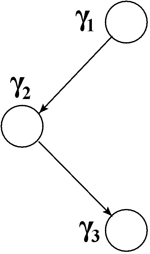
Figure 13: A BPS quiver for the ($A_{1},D_{3}$) Argyres-Douglas theory.

We consider $(A_{1},D_{3})$ Argyres-Douglas theory. This is equivalently the $(A_{1},A_{3})$ Argyres-Douglas theory. Line defect generators and their generating functions in this description were studied in Cordova:2016uwk ; Gaiotto:2010be . Line defect Schur indices and the relation to the Verlinde algebra were studied in Cordova:2016uwk . Here we use the $(A_{1},D_{3})$ description instead.

We choose a chamber where the BPS quiver is as in Figure 13, containing BPS particles with charges (in increasing phase order):

$$\gamma_{1},\gamma_{2},\gamma_{3}.$$

Note that $\gamma_{1}+\gamma_{3}$ has zero Dirac pairing with any charge, and thus is a pure flavor charge.

The corresponding Hitchin system is defined on $\mathbb{CP}^{1}$, with one irregular singularity at $z=\infty$ and one regular singularity at $z=0$. There are three Stokes rays emerging from the irregular singularity. Correspondingly there are three marked points on the $S^{1}$ bounding the cut-out disc around $z=\infty$, as in Figure 14(a). The WKB triangulation for the chosen chamber is shown in Figure 14(b). Here ${\mathcal{X}}_{\gamma_{1}}$ corresponds to edge 14, ${\mathcal{X}}_{\gamma_{2}}$ corresponds to edge 13, and ${\mathcal{X}}_{\gamma_{3}}$ corresponds to edge 34.

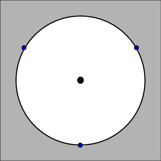
(a)

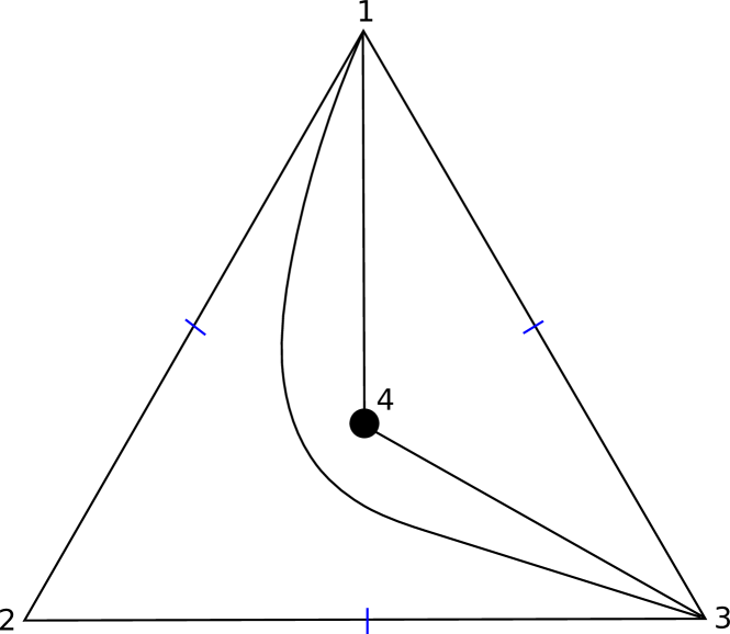
(b)

Figure 14: (a): $\mathbb{CP}^{1}\setminus D_{\infty}$ where $D_{\infty}$ is a disk around $z=\infty$ bounded by $S^{1}$ with three marked points colored in blue. The regular singularity at $z=0$ is colored in black. (b): A triangulation in the $(A_{1},D_{3})$ Argyres-Douglas theory. There are three boundary edges. The blue marks correspond to the positions of three Stokes rays.

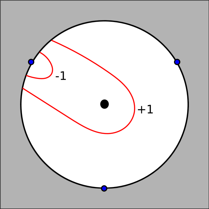
(a) Type $A$

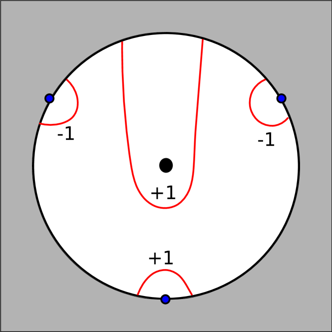
(b) Type $B$

(c) Type $C$

Figure 15: Three types of laminations in $(A_{1},D_{3})$ Argyres-Douglas theory.

Now we use the method reviewed in §4.3 to describe a generating set of line defects. There are seven generators, including a pure flavor line defect $C$ whose corresponding lamination is a loop around the regular singularity. The other six generators come in two types, $A$ and $B$, corresponding to two different kinds of laminations: see Figure 15. We denote the six generators as $A_{i},B_{i}\ (i=1,2,3)$, where $A_{1}$ and $B_{1}$ correspond to the laminations shown in Figure 15. The lamination for $A_{i+1}$ ($B_{i+1}$) is given by rotating the lamination for $A_{i}$ ($B_{i}$) counterclockwise by $2\pi/3$. The flavor charge is normalized to be $(\gamma_{1}+\gamma_{3})/2$, and the corresponding $X_{\gamma}$ is equal to the $SU(2)$ flavor fugacity $z$:

$$z=X_{\frac{\gamma_{1}+\gamma_{3}}{2}}.$$ (138)

Moreover we define

$$X_{\gamma^{\prime}}:=X_{\frac{\gamma_{1}-\gamma_{3}}{2}}.$$ (139)

We computed generating functions of line defect generators using the method reviewed in §4.3. They are listed below (these differ slightly from the analogous formulas in Cordova:2016uwk because we are computing in a different chamber):

$$F({A_{1}}) =z^{-1}X_{-{\gamma_{2}}}+X_{-\gamma^{\prime}}+X_{-\gamma^{\prime}-\gamma_{2}},$$

$$F({A_{2}}) =X_{-\gamma^{\prime}}+X_{-\gamma^{\prime}+\gamma_{2}}+zX_{\gamma_{2}},$$

$$F({A_{3}}) =X_{\gamma^{\prime}},$$

$$F({B_{1}}) =X_{-\gamma_{2}}+z^{-1}X_{-\gamma_{2}+\gamma^{\prime}},$$

$$F({B_{2}}) =X_{-2\gamma^{\prime}+\gamma_{2}}+X_{-2\gamma^{\prime}-\gamma_{2}}+zX_{-\gamma^{\prime}+\gamma_{2}}+(q^{\frac{1}{2}}+q^{-\frac{1}{2}})X_{-2\gamma^{\prime}}+(z+z^{-1})X_{-\gamma^{\prime}}+z^{-1}X_{-\gamma^{\prime}-\gamma_{2}},$$

$$F({B_{3}}) =X_{\gamma_{2}}+zX_{\gamma_{2}+\gamma^{\prime}},$$

$$F(C) =z+z^{-1}.$$

The pure flavor line defect $C$ is a Wilson line in the fundamental representation of the $SU(2)$ flavor symmetry.

The Schur index with one line defect $L$ inserted is computed as

$${\mathcal{I}}_{L}(q,z)=(q)_{\infty}^{2}\text{Tr}[F(L)S(q)\overline{S}(q)],\quad\text{with}\quad S(q)=E_{q}(X_{\gamma_{1}})E_{q}(X_{\gamma_{2}})E_{q}(X_{\gamma_{3}}).$$ (140)

As usual the Schur indices with defects $A_{i}$ and $B_{i}$ inserted do not depend on the index $i$; concretely (these do match Cordova:2016uwk , as they should since they are chamber-independent):

$${\mathcal{I}}_{A}(q,z) =-q^{\frac{1}{2}}(\chi_{\textbf{2}}+\chi_{\textbf{4}}q+\chi_{\bf{2\oplus 4\oplus 6}}q^{2}+\chi_{\bf{2}^{\oplus\text{2}}\oplus 4^{\oplus\text{2}}\oplus\bf{6}\oplus\bf{8}}q^{3}+\chi_{\bf{2^{\oplus\text{3}}\oplus 4^{\oplus\text{3}}\oplus 6^{\oplus\text{3}}\oplus 8\oplus 10}}q^{4}$$

$$\ \ +\chi_{\bf{2^{\oplus\text{4}}\oplus 4^{\oplus\text{6}}\oplus 6^{\oplus\text{4}}\oplus 8^{\oplus\text{3}}\oplus 10\oplus 12}}q^{5}+\cdots),$$

$${\mathcal{I}}_{B}(q,z) =-q^{\frac{1}{2}}(1+\chi_{\bf{3}}q^{2}+\chi_{\bf{1\oplus 3}}q^{3}+\chi_{\bf{1\oplus 3\oplus 5}}q^{4}+\chi_{\bf{1\oplus 3^{\oplus\text{2}}\oplus 5}}q^{5}+\chi_{\bf{1^{\oplus\text{2}}\oplus 3^{\oplus\text{3}}\oplus 5^{\oplus\text{2}}\oplus 7}}q^{6}+\cdots),$$

where framed BPS states organize themselves into representations of $SU(2)$.

The associated chiral algebra is $\widehat{\mathfrak{sl}(2)}_{-\frac{4}{3}}$Beem:2013sza ; Beem:2014zpa ; Cordova:2015nma ; Buican:2015ina ; Xie:2016evu . There are three admissible representations D.Francesco ; V.G.Kac with highest weights:

$$\Phi_{0}=\left[-\frac{4}{3},0\right],\quad\Phi_{1}=\left[-\frac{2}{3},-\frac{2}{3}\right],\quad\Phi_{2}=\left[0,-\frac{4}{3}\right]$$ (141)

where $\Phi_{0}$ is the highest weight for the vacuum module. Their characters were computed using the Kazhdan-Lusztig formula in D.Francesco ; Cordova:2016uwk . In particular the line defect Schur indices could be written as:

$$\begin{split}{\mathcal{I}}_{A}(q,z)&=q^{-\frac{1}{2}}z^{-1}\big{(}-\chi_{1}(q,z)+\chi_{2}(q,z)\big{)},\\ {\mathcal{I}}_{B}(q,z)&=q^{-\frac{1}{2}}\big{(}\chi_{0}(q,z)-\chi_{1}(q,z)+z^{-2}\chi_{2}(q,z)\big{)}.\end{split}$$ (142)

The expansions of ${\mathcal{I}}_{A_{i}A_{j}}$, ${\mathcal{I}}_{B_{i}B_{j}}$ and ${\mathcal{I}}_{A_{i}B_{j}}$ in terms of characters are:

$${\mathcal{I}}_{A_{i}A_{i}}(q,z)={\mathcal{I}}_{A_{i}A_{i+1}}(q,z) =(1+q^{-1})\chi_{0}(q,z)-q^{-1}\chi_{1}(q,z)+q^{-1}z^{-2}\chi_{2}(q,z),$$

$${\mathcal{I}}_{A_{i}A_{i-1}}(q,z) =2\chi_{0}(q,z)-\chi_{1}(q,z)+z^{-2}\chi_{2}(q,z),$$

$${\mathcal{I}}_{B_{i}B_{i}}(q,z)={\mathcal{I}}_{B_{i}B_{i+1}}(q,z) =(1+q^{-1}+q^{-2})\chi_{0}(q,z)-[q^{-1}(1+z^{-2})+q^{-2}]\chi_{1}(q,z)$$

$$\ \ +[q^{-1}(1+z^{-2})+q^{-2}z^{-2}]\chi_{2}(q,z),$$

$${\mathcal{I}}_{B_{i}B_{i-1}}(q,z) =(2+q)\chi_{0}(q,z)-(2+z^{-2})\chi_{1}(q,z)+(1+2z^{-2})\chi_{2}(q,z),$$

$${\mathcal{I}}_{A_{i}B_{i}}(q,z) =q^{-1}(z+z^{-1})\chi_{0}(q,z)-(q^{-1}+q^{-2})z^{-1}\big{(}\chi_{1}(q,z)-\chi_{2}(q,z)\big{)},$$

$${\mathcal{I}}_{A_{i}B_{i+1}}(q,z)={\mathcal{I}}_{A_{i}B_{i-1}}(q,z) =(z+z^{-1})\chi_{0}(q,z)-(1+q^{-1})z^{-1}\big{(}\chi_{1}(q,z)-\chi_{2}(q,z)\big{)}.$$

In Cordova:2016uwk the authors take the limit $q\to 1,z\to 1$ and relate the line defect algebra to the Verlinde-like algebra of $\widehat{\mathfrak{sl}(2)}_{-\frac{4}{3}}$. Here we keep $z$ general while taking $q\to 1$. In this limit the expansion coefficients do not depend on the $i$ index anymore, just as in the $(A_{1},A_{2N})$ case. We introduce a $z$-deformed Verlinde-like algebra ${\mathcal{V}}_{z}$ with the $z$-deformed modular fusion rules:

$$\begin{split}[\Phi_{1}]\times[\Phi_{1}]&=[\Phi_{2}],\\ [\Phi_{1}]\times[\Phi_{2}]&=-z^{2}[\Phi_{0}],\\ [\Phi_{2}]\times[\Phi_{2}]&=-z^{2}[\Phi_{1}].\end{split}$$ (143)

If we take $z=1$, this reduces to the naive modular fusion rules of $\widehat{\mathfrak{sl}(2)}_{-\frac{4}{3}}$ D.Francesco ; Cordova:2016uwk . The homomorphism $f:{\mathcal{L}}\to{\mathcal{V}}_{z}$ is given by:

$$\begin{split}I&\xrightarrow{f}[\Phi_{0}],\\ A_{i}&\xrightarrow{f}[A]=z^{-1}\big{(}[\Phi_{2}]-[\Phi_{1}]\big{)},\\ B_{i}&\xrightarrow{f}[B]=[\Phi_{0}]-[\Phi_{1}]+z^{-2}[\Phi_{2}].\end{split}$$ (144)

$f$ is believed to be a homomorphism since

$$\begin{split}[AA]&=2[\Phi_{0}]-[\Phi_{1}]+z^{-2}[\Phi_{2}]=[A]\times[A],\\ [BB]&=3[\Phi_{0}]-(2+z^{-2})[\Phi_{1}]+(1+2z^{-2})[\Phi_{2}]=[B]\times[B],\\ [AB]&=(z+z^{-1})[\Phi_{0}]-2z^{-1}\big{(}[\Phi_{1}]-[\Phi_{2}]\big{)}=[A]\times[B].\end{split}$$ (145)

We emphasize that this holds if and only if the $z$-deformed modular fusion rules are as given in (143).

The fusion matrices for $[\Phi_{1}]$ and $[\Phi_{2}]$ are:

$$N_{\Phi_{1}}=\begin{pmatrix}0&1&0\\ 0&0&1\\ -z^{2}&0&0\end{pmatrix},\quad N_{\Phi_{2}}=\begin{pmatrix}0&0&1\\ -z^{2}&0&0\\ 0&-z^{2}&0\end{pmatrix}.$$ (146)

These two matrices are simultaneously diagonalizable for $z\neq 0$, with eigenvalues:

eigenvector	$\lambda_{\Phi_{1}}$	$\lambda_{\Phi_{2}}$
$(1,-z^{2/3},z^{4/3})$	$-z^{2/3}$	$z^{4/3}$
$(1,(-1)^{1/3}z^{2/3},(-1)^{2/3}z^{4/3})$	$(-1)^{1/3}z^{2/3}$	$(-1)^{2/3}z^{4/3}$
$(1,-(-1)^{2/3}z^{2/3},-(-1)^{1/3}z^{4/3})$	$-(-1)^{2/3}z^{2/3}$	$-(-1)^{1/3}z^{4/3}$

Figure 16: Classical monodromy action via two flips in $(A_{1},D_{3})$ Argyres-Douglas theory.

Now we turn to study fixed loci of the classical monodromy in this chamber. Through a composition of two flips (see Figure 16) the monodromy action is:

$$\begin{split}&{\mathcal{X}}_{\gamma_{1}}\to\frac{1+{\mathcal{X}}_{\gamma_{3}}+{\mathcal{X}}_{\gamma_{2}}{\mathcal{X}}_{\gamma_{3}}}{{\mathcal{X}}_{\gamma_{2}}},\\ &{\mathcal{X}}_{\gamma_{2}}\to\frac{1}{{\mathcal{X}}_{\gamma_{3}}+{\mathcal{X}}_{\gamma_{2}}{\mathcal{X}}_{\gamma_{3}}},\\ &{\mathcal{X}}_{\gamma_{3}}\to\frac{{\mathcal{X}}_{\gamma_{1}}{\mathcal{X}}_{\gamma_{2}}{\mathcal{X}}_{\gamma_{3}}}{1+{\mathcal{X}}_{\gamma_{3}}+{\mathcal{X}}_{\gamma_{2}}{\mathcal{X}}_{\gamma_{3}}}.\end{split}$$ (147)

The fixed locus is determined by the equations

$${\mathcal{X}}_{\gamma_{2}}(1+{\mathcal{X}}_{\gamma_{2}}){\mathcal{X}}_{\gamma_{3}}=1,\quad{\mathcal{X}}_{\gamma_{1}}={\mathcal{X}}_{\gamma_{3}}(2+{\mathcal{X}}_{\gamma_{2}}+{\mathcal{X}}_{\gamma_{3}}+{\mathcal{X}}_{\gamma_{2}}{\mathcal{X}}_{\gamma_{3}}).$$ (148)

To make connection with the flavor fugacity, we rewrite these equations in terms of ${\mathcal{X}}_{\gamma_{2}}$, $z$ and $x:={\mathcal{X}}_{\gamma^{\prime}}$; this gives

$${\mathcal{X}}_{\gamma_{2}}^{3}z^{2}=1,\quad x={\mathcal{X}}_{\gamma_{2}}(1+{\mathcal{X}}_{\gamma_{2}})z.$$ (149)

One can check that this is exactly the same locus where $F({A_{i}})=F({A_{j}})$ and $F({B_{i}})=F({B_{j}})$. In particular, this implies the evaluation map $g$ forgets the $i$ index as expected.

Now recall that the value of $z$ corresponds to the $SU(2)$ flavor holonomy that could be turned on when compactifying the 4d theory on $S^{1}$. With this in mind we first fix $z$ and then look for the $U(1)_{r}$-fixed points. For each value of $z\neq 0$, there are three $U(1)_{r}$-fixed points, which matches the number of admissible representations of $\widehat{\mathfrak{sl}(2)}_{-\frac{4}{3}}$. The evaluation map $g$ is concretely given by:

$$\begin{split}1&\xrightarrow{g}\big{(}1,1,1\big{)},\\ A_{i}&\xrightarrow{g}\big{(}z^{1/3}+z^{-1/3},-(-1)^{1/3}z^{1/3}+(-1)^{2/3}z^{-1/3},-(-1)^{1/3}z^{-1/3}+(-1)^{2/3}z^{1/3}\big{)},\\ B_{i}&\xrightarrow{g}\big{(}1+z^{2/3}+z^{-2/3},1+(-1)^{2/3}z^{2/3}-(-1)^{1/3}z^{-2/3},\\ &\ \ \ \ \ 1+(-1)^{2/3}z^{-2/3}-(-1)^{1/3}z^{2/3}\big{)}.\end{split}$$ (150)

Now, in contrast to the cases we studied in §5, in this case the weights of the classical monodromy action are not sufficient to distinguish the three $U(1)_{r}$-fixed points, as we see from the following table ($U(1)_{r}$ weights and correspondence between fixed points and primary fields taken from results of Fredrickson-Neitzke ; Fredrickson:2017yka ):

fixed point	weights of $M$	weights of $U(1)_{r}$	primary field
I	$-\frac{1\pm{\mathrm{i}}\sqrt{3}}{2}$	$\frac{1}{3},\frac{2}{3}$	$\Phi_{1}$
II	$-\frac{1\pm{\mathrm{i}}\sqrt{3}}{2}$	$-\frac{1}{3},\frac{4}{3}$	$\Phi_{0}$
III	$-\frac{1\pm{\mathrm{i}}\sqrt{3}}{2}$	$-\frac{1}{3},\frac{4}{3}$	$\Phi_{2}$

Thus we cannot determine a priori which $U(1)_{r}$-fixed point should correspond to which eigenspace of the fusion matrices. This gives an $S_{3}$ ambiguity in constructing the map $h$. Still, we can just try all of the $6$ possible mappings and see if one of them works. Indeed, suppose we take:

$$\begin{split}[\Phi_{1}]&\xrightarrow{h}\big{(}-z^{2/3},-(-1)^{2/3}z^{2/3},(-1)^{1/3}z^{2/3}\big{)},\\ [\Phi_{2}]&\xrightarrow{h}\big{(}z^{4/3},-(-1)^{1/3}z^{4/3},(-1)^{2/3}z^{4/3}\big{)}.\end{split}$$ (151)

Combining this with (144) and (150), we find that indeed $h\circ f=g$ for every $z\neq 0$.

6.2 $(A_{1},D_{5})$ Argyres-Douglas theory

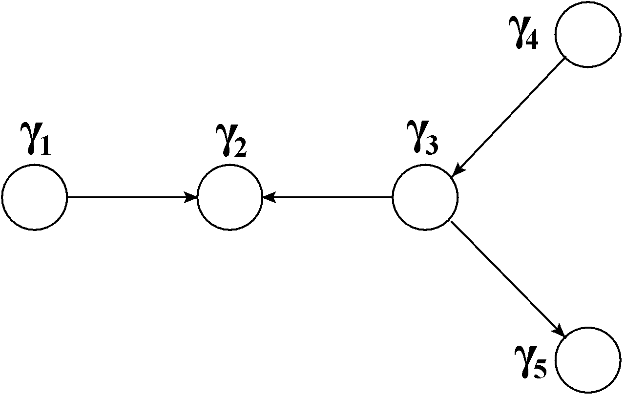
Figure 17: A BPS quiver for the ($A_{1},D_{5}$) Argyres-Douglas theory.

We choose the canonical chamber represented by the BPS quiver given in Figure 17, with five BPS particles (in increasing central charge phase order):

$$\gamma_{1},\gamma_{4},\gamma_{3},\gamma_{2},\gamma_{5}.$$

The corresponding Hitchin system is defined on $\mathbb{CP}^{1}$ with one regular singularity at $z=0$ and one irregular singularity at $z=\infty$ with five stokes rays emerging from it, i.e. there are five marked points on the $S^{1}$ which bounds $D_{\infty}$, the disk around $z=\infty$ that’s cut out from $\mathbb{CP}^{1}$. The situation is depicted in Figure 18. The corresponding WKB triangulation for this chamber is given in Figure 19, where ${\mathcal{X}}_{\gamma_{1}}$ corresponds to edge 13, ${\mathcal{X}}_{\gamma_{2}}$ corresponds to edge 35, ${\mathcal{X}}_{\gamma_{3}}$ corresponds to edge 45, ${\mathcal{X}}_{\gamma_{4}}$ corresponds to edge 56 and ${\mathcal{X}}_{\gamma_{5}}$ corresponds to edge 46.

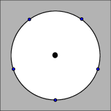
Figure 18: $\mathbb{CP}^{1}\setminus D_{\infty}$ where $D_{\infty}$ is a disk around $z=\infty$ bounded by $S^{1}$ with five marked points colored in blue. The regular singularity at $z=0$ is colored in black.

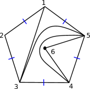
Figure 19: A triangulation in the $(A_{1},D_{5})$ Argyres-Douglas theory. There are five boundary edges. The blue marks correspond to positions of five Stokes rays.

The line defect generators correspond to laminations that can not be expressed as sum of other laminations. In this case there are 21 such laminations. The lamination ($E$) which is a loop around the regular singularity corresponds to the pure flavor line defect. The other 20 laminations come in four types $A,B,C$ and $D$. We label their corresponding generators as $A_{i}$, $B_{i}$, $C_{i}$ and $D_{i}$ ($i=1,\dots,5$) and list laminations corresponding to the generators $A_{1},B_{1},C_{1},D_{1}$ and $E$ in Figure 20. Laminations corresponding to e.g. generators $A_{i+1}$ are obtained by rotating laminations for $A_{i}$ clockwise by $4\pi/5$.

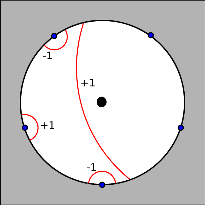
(a) Type A

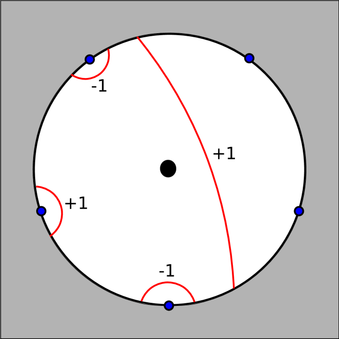
(b) Type B

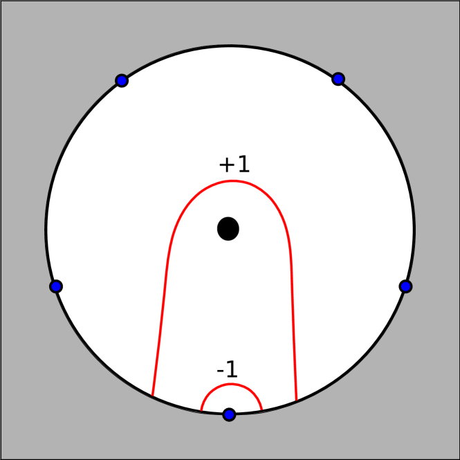
(c) Type C

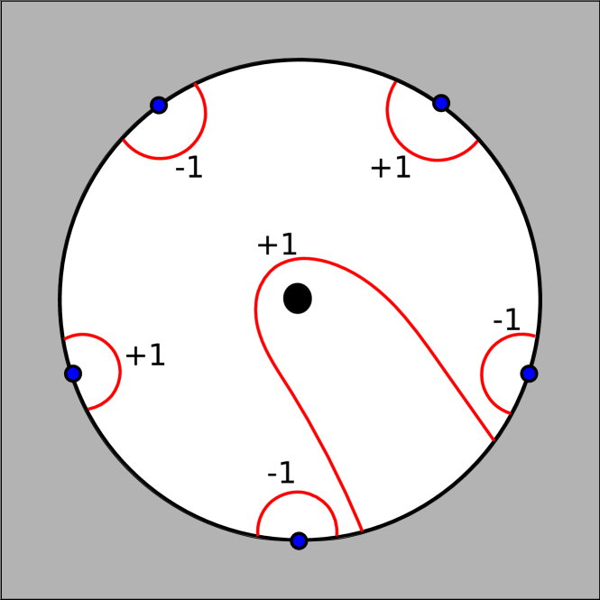
(d) Type D

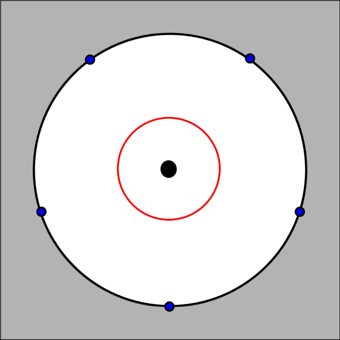
(e) Type E

Figure 20: Five types of laminations in $(A_{1},D_{5})$ Argyres-Douglas theory.

We define the flavor charge $\gamma_{f}$ and $\gamma^{\prime}$ as follows:

$$\gamma_{f}=\frac{\gamma_{4}+\gamma_{5}}{2},\quad\gamma^{\prime}=\frac{\gamma_{4}-\gamma_{5}}{2}.$$ (152)

The $SU(2)$ flavor fugacity is $z:=\text{Tr}(X_{\gamma_{f}})$. The generating functions are computed using the method as reviewed in §4.3. In particular, the line defect generator $D_{2}$ has framed BPS states with charge $2\gamma_{2}$ in a 3-dimensional multiplet of $SO(3)$:

$$F(A_{1}) =X_{-\gamma_{1}}+X_{-\gamma_{1}-\gamma_{2}},$$

$$F(A_{2}) =X_{-\gamma_{1}}+X_{\gamma_{2}}+X_{-\gamma_{1}+\gamma_{2}}+X_{\gamma_{2}+\gamma_{3}}+X_{-\gamma_{1}+\gamma_{2}+\gamma_{3}}+zX_{\gamma_{2}+\gamma_{3}+\gamma^{\prime}}+zX_{-\gamma_{1}+\gamma_{2}+\gamma_{3}+\gamma^{\prime}},$$

$$F(A_{3}) =X_{\gamma_{2}}+X_{\gamma_{1}+\gamma_{2}}+X_{-\gamma_{3}}+X_{\gamma_{2}-\gamma_{3}}+X_{\gamma_{1}+\gamma_{2}-\gamma_{3}}+z^{-1}X_{-\gamma_{3}+\gamma^{\prime}}+z^{-1}X_{\gamma_{2}-\gamma_{3}+\gamma^{\prime}}$$

$$\ \ +z^{-1}X_{\gamma_{1}+\gamma_{2}-\gamma_{3}+\gamma^{\prime}},$$

$$F(A_{4}) =X_{\gamma_{1}},$$

$$F(A_{5}) =(z+z^{-1})X_{-\gamma^{\prime}}+z^{-1}X_{-\gamma_{3}-\gamma^{\prime}}+z^{-1}X_{-\gamma_{2}-\gamma_{3}-\gamma^{\prime}}+zX_{\gamma_{3}-\gamma^{\prime}}+(q^{1/2}+q^{-1/2})X_{-2\gamma^{\prime}}$$

$$\ \ +X_{-\gamma_{2}-2\gamma^{\prime}}+X_{-\gamma_{3}-2\gamma^{\prime}}+X_{-\gamma_{2}-\gamma_{3}-2\gamma^{\prime}}+X_{\gamma_{3}-2\gamma^{\prime}},$$

$$F(B_{1}) =X_{-\gamma_{1}-\gamma^{\prime}}+X_{-\gamma_{1}-\gamma_{2}-\gamma^{\prime}}+X_{-\gamma_{1}+\gamma_{3}-\gamma^{\prime}}+zX_{-\gamma_{1}+\gamma_{3}},$$

$$F(B_{2}) =X_{-\gamma_{1}+\gamma^{\prime}}+X_{\gamma_{2}+\gamma^{\prime}}+X_{-\gamma_{1}+\gamma_{2}+\gamma^{\prime}},$$

$$F(B_{3}) =X_{\gamma_{2}+\gamma^{\prime}}+X_{\gamma_{1}+\gamma_{2}+\gamma^{\prime}},$$

$$F(B_{4}) =z^{-1}X_{\gamma_{1}-\gamma_{3}}+X_{\gamma_{1}-\gamma^{\prime}}+X_{\gamma_{1}-\gamma_{3}-\gamma^{\prime}},$$

$$F(B_{5}) =X_{-\gamma_{2}-\gamma^{\prime}},$$

$$F(C_{1}) =X_{-\gamma^{\prime}}+X_{\gamma_{3}-\gamma^{\prime}}+zX_{\gamma_{3}},$$

$$F(C_{2}) =(q^{1/2}+q^{-1/2})\big{(}X_{-\gamma_{1}-\gamma^{\prime}}+X_{\gamma_{2}-\gamma^{\prime}}+X_{-\gamma_{1}+\gamma_{2}-\gamma^{\prime}}+X_{-\gamma_{1}-\gamma_{3}-\gamma^{\prime}}+z^{-1}X_{-\gamma_{1}-\gamma_{3}}\big{)}$$

$$\ \ +X_{-\gamma^{\prime}}+X_{-\gamma_{3}-\gamma^{\prime}}+X_{-\gamma_{1}-\gamma_{2}-\gamma_{3}-\gamma^{\prime}}+X_{\gamma_{2}-\gamma_{3}-\gamma^{\prime}}+X_{-\gamma_{1}+\gamma_{2}-\gamma_{3}-\gamma^{\prime}}+X_{\gamma_{2}+\gamma_{3}-\gamma^{\prime}}$$

$$\ \ +X_{-\gamma_{1}+\gamma_{2}+\gamma_{3}-\gamma^{\prime}}+(z+z^{-1})X_{-\gamma_{1}}+(z+z^{-1})X_{\gamma_{2}}+(z+z^{-1})X_{-\gamma_{1}+\gamma_{2}}+z^{-1}X_{-\gamma_{3}}$$

$$\ \ +z^{-1}X_{-\gamma_{1}-\gamma_{2}-\gamma_{3}}+z^{-1}X_{\gamma_{2}-\gamma_{3}}+z^{-1}X_{-\gamma_{1}+\gamma_{2}-\gamma_{3}}+zX_{\gamma_{2}+\gamma_{3}}+zX_{-\gamma_{1}+\gamma_{2}+\gamma_{3}},$$

$$F(C_{3}) =X_{\gamma^{\prime}},$$

$$F(C_{4}) =(q^{1/2}+q^{-1/2})\big{(}X_{\gamma_{2}-\gamma^{\prime}}+X_{\gamma_{1}+\gamma_{2}-\gamma^{\prime}}\big{)}+X_{-\gamma^{\prime}}+X_{-\gamma_{3}-\gamma^{\prime}}+X_{\gamma_{2}-\gamma_{3}-\gamma^{\prime}}+X_{\gamma_{1}+\gamma_{2}-\gamma_{3}-\gamma^{\prime}}$$

$$\ \ +X_{\gamma_{2}+\gamma_{3}-\gamma^{\prime}}+X_{\gamma_{1}+\gamma_{2}+\gamma_{3}-\gamma^{\prime}}+z^{-1}X_{\gamma_{2}}+z^{-1}X_{\gamma_{1}+\gamma_{2}}+z^{-1}X_{-\gamma_{3}}+z^{-1}X_{\gamma_{2}-\gamma_{3}}$$

$$\ \ +z^{-1}X_{\gamma_{1}+\gamma_{2}-\gamma_{3}}+zX_{\gamma_{2}}+zX_{\gamma_{1}+\gamma_{2}}+zX_{\gamma_{2}+\gamma_{3}}+zX_{\gamma_{1}+\gamma_{2}+\gamma_{3}},$$

$$F(C_{5}) =X_{-\gamma^{\prime}}+X_{-\gamma_{3}-\gamma^{\prime}}+X_{-\gamma_{2}-\gamma_{3}-\gamma^{\prime}}+z^{-1}X_{-\gamma_{3}}+z^{-1}X_{-\gamma_{2}-\gamma_{3}},$$

$$F(D_{1}) =X_{-\gamma_{1}+\gamma_{3}}+zX_{-\gamma_{1}+\gamma_{3}+\gamma^{\prime}},$$

$$F(D_{2}) =(q^{1/2}+q^{-1/2})X_{\gamma_{2}}+(q^{1/2}+q^{-1/2})X_{-\gamma_{1}+\gamma_{2}}+(1+1+q+q^{-1})X_{2\gamma_{2}}$$

$$\ \ +(q^{1/2}+q^{-1/2})X_{-\gamma_{1}+2\gamma_{2}}+(q^{1/2}+q^{-1/2})X_{\gamma_{1}+2\gamma_{2}}+X_{-\gamma_{1}-\gamma_{3}}+(q^{1/2}+q^{-1/2})X_{\gamma_{2}-\gamma_{3}}$$

$$\ \ +(q^{1/2}+q^{-1/2})X_{-\gamma_{1}+\gamma_{2}-\gamma_{3}}+(q^{1/2}+q^{-1/2})X_{2\gamma_{2}-\gamma_{3}}+X_{-\gamma_{1}+2\gamma_{2}-\gamma_{3}}+X_{\gamma_{1}+2\gamma_{2}-\gamma_{3}}$$

$$\ \ +(q^{1/2}+q^{-1/2})X_{2\gamma_{2}+\gamma_{3}}+X_{-\gamma_{1}+2\gamma_{2}+\gamma_{3}}+X_{\gamma_{1}+2\gamma_{2}+\gamma_{3}}+(z+z^{-1})X_{\gamma_{2}+\gamma^{\prime}}$$

$$\ \ +(z+z^{-1})X_{-\gamma_{1}+\gamma_{2}+\gamma^{\prime}}+(z+z^{-1})(q^{1/2}+q^{-1/2})X_{2\gamma_{2}+\gamma^{\prime}}+(z+z^{-1})X_{-\gamma_{1}+2\gamma_{2}+\gamma^{\prime}}$$

$$\ \ +(z+z^{-1})X_{\gamma_{1}+2\gamma_{2}+\gamma^{\prime}}+z^{-1}X_{-\gamma_{1}-\gamma_{3}+\gamma^{\prime}}+(q^{1/2}+q^{-1/2})z^{-1}X_{\gamma_{2}-\gamma_{3}+\gamma^{\prime}}$$

$$\ \ +(q^{1/2}+q^{-1/2})z^{-1}X_{-\gamma_{1}+\gamma_{2}-\gamma_{3}+\gamma^{\prime}}+(q^{1/2}+q^{-1/2})z^{-1}X_{2\gamma_{2}-\gamma_{3}+\gamma^{\prime}}+z^{-1}X_{-\gamma_{1}+2\gamma_{2}-\gamma_{3}+\gamma^{\prime}}$$

$$\ \ +z^{-1}X_{\gamma_{1}+2\gamma_{2}-\gamma_{3}+\gamma^{\prime}}+(q^{1/2}+q^{-1/2})zX_{2\gamma_{2}+\gamma_{3}+\gamma^{\prime}}+zX_{-\gamma_{1}+2\gamma_{2}+\gamma_{3}+\gamma^{\prime}}+zX_{\gamma_{1}+2\gamma_{2}+\gamma_{3}+\gamma^{\prime}},$$

$$F(D_{3}) =X_{\gamma_{1}-\gamma_{3}}+z^{-1}X_{\gamma_{1}-\gamma_{3}+\gamma^{\prime}},$$

$$F(D_{4}) =(q^{1/2}+q^{-1/2})X_{\gamma_{1}-2\gamma^{\prime}}+X_{\gamma_{1}-\gamma_{3}-2\gamma^{\prime}}+X_{\gamma_{1}+\gamma_{3}-2\gamma^{\prime}}+z^{-1}X_{\gamma_{1}-\gamma^{\prime}}+z^{-1}X_{\gamma_{1}-\gamma_{3}-\gamma^{\prime}}$$

$$\ \ +zX_{\gamma_{1}-\gamma^{\prime}}+zX_{\gamma_{1}+\gamma_{3}-\gamma^{\prime}},$$

$$F(D_{5}) =(q^{1/2}+q^{-1/2})\big{(}X_{-\gamma_{1}-2\gamma^{\prime}}+X_{-\gamma_{1}-\gamma_{2}-2\gamma^{\prime}}+X_{-\gamma_{1}-\gamma_{2}-\gamma_{3}-2\gamma^{\prime}}+z^{-1}X_{-\gamma_{1}-\gamma_{2}-\gamma_{3}-\gamma^{\prime}}\big{)}$$

$$\ \ +X_{-\gamma_{1}-\gamma_{3}-2\gamma^{\prime}}+X_{-\gamma_{1}-2\gamma_{2}-\gamma_{3}-2\gamma^{\prime}}+X_{-\gamma_{1}+\gamma_{3}-2\gamma^{\prime}}+(z+z^{-1})X_{-\gamma_{1}-\gamma^{\prime}}$$

$$\ \ +(z+z^{-1})X_{-\gamma_{1}-\gamma_{2}-\gamma^{\prime}}+z^{-1}X_{-\gamma_{1}-\gamma_{3}-\gamma^{\prime}}+z^{-1}X_{-\gamma_{1}-2\gamma_{2}-\gamma_{3}-\gamma^{\prime}}+zX_{-\gamma_{1}+\gamma_{3}-\gamma^{\prime}},$$

$$F(E) =z+z^{-1}.$$

The line defect Schur index is

$$\begin{split}{\mathcal{I}}_{L}(q,z)&=(q)_{\infty}^{4}\text{Tr}[F(L)S(q)\overline{S}(q)],\quad\text{with}\\ S(q)&=E_{q}(X_{\gamma_{1}})E_{q}(X_{\gamma_{4}})E_{q}(X_{\gamma_{3}})E_{q}(X_{\gamma_{2}})E_{q}(X_{\gamma_{5}}).\end{split}$$ (153)

After inserting generating functions the calculation boils down to computing the following:

$$\ \ \ (q)_{\infty}^{4}\text{Tr}[X_{a\gamma_{1}+b\gamma_{2}+c\gamma_{3}+d\gamma^{\prime}}S(q)\overline{S}(q)]$$

$$=(q)_{\infty}^{4}\displaystyle\sum\limits_{l_{i},k_{i}=0}^{\infty}\frac{(-1)^{a+b+c+d}q^{A/2}z^{l_{4}+l_{5}-k_{4}-k_{5}}}{(q)_{l_{1}}\dots(q)_{l_{5}}(q)_{k_{1}}\dots(q)_{k_{5}}}\delta_{k_{1},l_{1}+a}\delta_{k_{2},l_{2}+b}\delta_{k_{3},l_{3}+c}\delta_{k_{4},l_{4}-l_{5}+k_{5}+d},\quad\text{with}$$

$$A=\frac{1}{2}\Big{(}a+b+ab+c+bc-cd+d(1+2c+2l_{3})+2\big{(}l_{1}+l_{2}+al_{2}+cl_{2}+l_{1}l_{2}+l_{3}$$

$$\quad\quad+l_{2}l_{3}+k_{5}(1+c+l_{3})+l_{4}+l_{3}l_{4}\big{)}\Big{)}.$$

Within the same class line defect Schur indices are the same. The coefficients in $q$ are again characters of certain $SU(2)$ representations:

$$\begin{split}{\mathcal{I}}_{A}(q,z)&=-q^{\frac{1}{2}}(1+\chi_{\bf{3}}q+\chi_{\bf{1\oplus 3\oplus 5}}q^{2}+\chi_{\bf{1}\oplus 3^{\oplus\text{2}}\oplus 5\oplus 7}q^{3}+\cdots),\\ {\mathcal{I}}_{B}(q,z)&=q(\chi_{\bf{2}}+\chi_{\bf{4}}q+\chi_{\bf{2\oplus 4\oplus 6}}q^{2}+\chi_{\bf{2}^{\oplus\text{2}}\oplus 4^{\oplus\text{2}}\oplus 6\oplus 8}q^{3}+\cdots),\\ {\mathcal{I}}_{C}(q,z)&=-q^{\frac{1}{2}}(\chi_{\bf{2}}+\chi_{\bf{4}}q+\chi_{\bf{2}^{\oplus\text{2}}\oplus 4\oplus 6}q^{2}+\chi_{\bf{2}^{\oplus\text{2}}\oplus 4^{\oplus\text{3}}\oplus 6\oplus 8}q^{3}+\cdots),\\ {\mathcal{I}}_{D}(q,z)&=q(1+\chi_{\bf{3}}q^{2}+\chi_{\bf{1\oplus 3}}q^{3}+\cdots).\end{split}$$ (154)

The chiral algebra corresponding to the $(A_{1},D_{5})$ Argyres-Douglas theory is $\widehat{\mathfrak{sl}(2)}_{-\frac{8}{5}}$ Cordova:2015nma ; Beem:2013sza ; Beem:2014zpa ; Xie:2016evu , which has five admissible representations with the following highest weights:

$$\begin{split}\Phi_{0}&=\left[-\frac{8}{5},0\right],\quad\Phi_{1}=\left[-\frac{6}{5},-\frac{2}{5}\right],\quad\Phi_{2}=\left[-\frac{4}{5},-\frac{4}{5}\right],\\ \Phi_{3}&=\left[-\frac{2}{5},-\frac{6}{5}\right],\quad\Phi_{4}=\left[0,-\frac{8}{5}\right],\end{split}$$ (155)

where $\Phi_{0}$ is the highest weight for the vacuum module. The characters of these representations can be worked out using the Kac-Wakimoto formula V.G.Kac , which is a special case of the Kazhdan-Lusztig formula DeVos:1995an (see also D.Francesco for expressions in terms of generalized theta functions):

$$\begin{split}\chi_{0}(q,z)&=\frac{\sum_{m=0}^{\infty}(-1)^{m}\frac{z^{2m+1}-z^{-(2m+1)}}{z-z^{-1}}q^{\frac{5m(m+1)}{2}}}{\prod_{n=1}^{\infty}(1-q^{n})(1-z^{2}q^{n})(1-z^{-2}q^{n})},\\ \chi_{1}(q,z)&=\frac{1+\sum_{m=1}^{\infty}(-1)^{m}(z^{-2m}q^{\frac{m(5m-3)}{2}}+z^{2m}q^{\frac{m(5m+3)}{2}})}{(1-z^{-2})\prod_{n=1}^{\infty}(1-q^{n})(1-z^{2}q^{n})(1-z^{-2}q^{n})},\\ \chi_{2}(q,z)&=\frac{1+\sum_{m=1}^{\infty}(-1)^{m}(z^{-2m}q^{\frac{m(5m-1)}{2}}+z^{2m}q^{\frac{m(5m+1)}{2}})}{(1-z^{-2})\prod_{n=1}^{\infty}(1-q^{n})(1-z^{2}q^{n})(1-z^{-2}q^{n})},\\ \chi_{3}(q,z)&=\frac{1+\sum_{m=1}^{\infty}(-1)^{m}(z^{2m}q^{\frac{m(5m-1)}{2}}+z^{-2m}q^{\frac{m(5m+1)}{2}})}{(1-z^{-2})\prod_{n=1}^{\infty}(1-q^{n})(1-z^{2}q^{n})(1-z^{-2}q^{n})},\\ \chi_{4}(q,z)&=\frac{1+\sum_{m=1}^{\infty}(-1)^{m}(z^{2m}q^{\frac{m(5m-3)}{2}}+z^{-2m}q^{\frac{m(5m+3)}{2}})}{(1-z^{-2})\prod_{n=1}^{\infty}(1-q^{n})(1-z^{2}q^{n})(1-z^{-2}q^{n})}.\end{split}$$ (156)

The $\mathcal{S}$ matrix for these five admissible representations, in the order (155), is D.Francesco :

$$\mathcal{S}=\frac{1}{\sqrt{5}}\begin{pmatrix}1&-1&1&-1&1\\ -1&-(-1)^{3/5}&(-1)^{1/5}&(-1)^{4/5}&-(-1)^{2/5}\\ 1&(-1)^{1/5}&(-1)^{2/5}&(-1)^{3/5}&(-1)^{4/5}\\ -1&(-1)^{4/5}&(-1)^{3/5}&(-1)^{2/5}&(-1)^{1/5}\\ 1&-(-1)^{2/5}&(-1)^{4/5}&(-1)^{1/5}&-(-1)^{3/5}\end{pmatrix}.$$ (157)

Working out the conjugation matrix $\mathcal{C}=\mathcal{S}^{2}$ it’s clear that $\Phi_{1}$ and $\Phi_{4}$ are conjugate to each other, $\Phi_{2}$ and $\Phi_{3}$ are conjugate to each other. Using the Verlinde formula Verlinde:1988sn the modular fusion rules for $\widehat{\mathfrak{sl}(2)}_{-\frac{8}{5}}$ are given by:

$$\begin{split}[\Phi_{1}]\times[\Phi_{1}]&=[\Phi_{2}],\quad[\Phi_{1}]\times[\Phi_{2}]=[\Phi_{3}],\quad[\Phi_{1}]\times[\Phi_{3}]=[\Phi_{4}],\\ [\Phi_{1}]\times[\Phi_{4}]&=-[\Phi_{0}],\quad[\Phi_{2}]\times[\Phi_{2}]=[\Phi_{4}],\quad[\Phi_{2}]\times[\Phi_{3}]=-[\Phi_{0}],\\ [\Phi_{2}]\times[\Phi_{4}]&=-[\Phi_{1}],\quad[\Phi_{3}]\times[\Phi_{3}]=-[\Phi_{1}],\quad[\Phi_{3}]\times[\Phi_{4}]=-[\Phi_{2}],\\ [\Phi_{4}]\times[\Phi_{4}]&=-[\Phi_{3}].\end{split}$$ (158)

As we will see shortly, multiplications in the deformed Verlinde-like algebra are again given by multiplying the $-1$ coefficients in the original modular fusion rules by a factor of $z^{2}$.

The line defect Schur indices for defect generators of type $A$, $B$, $C$ and $D$ admit the following character expansions:

$$\begin{split}{\mathcal{I}}_{A}(q,z)&=q^{-1/2}\big{(}\chi_{0}(q,z)-\chi_{1}(q,z)+z^{-2}\chi_{4}(q,z)\big{)},\\ {\mathcal{I}}_{B}(q,z)&=q^{-1}z^{-1}\big{(}\chi_{2}(q,z)-\chi_{3}(q,z)\big{)},\\ {\mathcal{I}}_{C}(q,z)&=q^{-1/2}z^{-1}\big{(}-\chi_{1}(q,z)+\chi_{2}(q,z)-\chi_{3}(q,z)+\chi_{4}(q,z)\big{)},\\ {\mathcal{I}}_{D}(q,z)&=\chi_{0}(q,z)-q^{-1}\big{(}\chi_{1}(q,z)-\chi_{2}(q,z)+z^{-2}\chi_{3}(q,z)-z^{-2}\chi_{4}(q,z)\big{)}.\end{split}$$ (159)

Now we again take the $q\to 1$ limit while keeping $z$ general, giving the map

$$\begin{split}I&\xrightarrow{f}[\Phi_{0}],\\ A_{i}&\xrightarrow{f}[A]=[\Phi_{0}]-[\Phi_{1}]+z^{-2}[\Phi_{4}],\\ B_{i}&\xrightarrow{f}[B]=z^{-1}([\Phi_{2}]-[\Phi_{3}]),\\ C_{i}&\xrightarrow{f}[C]=z^{-1}(-[\Phi_{1}]+[\Phi_{2}]-[\Phi_{3}]+[\Phi_{4}]),\\ D_{i}&\xrightarrow{f}[D]=[\Phi_{0}]-[\Phi_{1}]+[\Phi_{2}]-z^{-2}[\Phi_{3}]+z^{-2}[\Phi_{4}].\end{split}$$ (160)

This map is believed to be a homomorphism $f:{\mathcal{L}}\to{\mathcal{V}}_{z}$, when we define the deformed Verlinde-like algebra ${\mathcal{V}}_{z}$ by the following $z$-deformed modular fusion rules:

$$\begin{split}[\Phi_{1}]\times[\Phi_{1}]&=[\Phi_{2}],\quad[\Phi_{1}]\times[\Phi_{2}]=[\Phi_{3}],\quad[\Phi_{1}]\times[\Phi_{3}]=[\Phi_{4}],\\ [\Phi_{1}]\times[\Phi_{4}]&=-z^{2}[\Phi_{0}],\quad[\Phi_{2}]\times[\Phi_{2}]=[\Phi_{4}],\quad[\Phi_{2}]\times[\Phi_{3}]=-z^{2}[\Phi_{0}],\\ [\Phi_{2}]\times[\Phi_{4}]&=-z^{2}[\Phi_{1}],\quad[\Phi_{3}]\times[\Phi_{3}]=-z^{2}[\Phi_{1}],\quad[\Phi_{3}]\times[\Phi_{4}]=-z^{2}[\Phi_{2}],\\ [\Phi_{4}]\times[\Phi_{4}]&=-z^{2}[\Phi_{3}].\end{split}$$ (161)

To check the homomorphism property we consider Schur indices with insertion of two half line defects, which can also be expanded in terms of characters of admissible representations. After setting $q\to 1$ the expansion coefficients do not depend on the $i$-index anymore:

$$A_{i}A_{j} \xrightarrow{f}3[\Phi_{0}]-2[\Phi_{1}]+[\Phi_{2}]-z^{-2}[\Phi_{3}]+2z^{-2}[\Phi_{4}],$$

$$A_{i}B_{j} \xrightarrow{f}z^{-1}(-[\Phi_{1}]+2[\Phi_{2}]-2[\Phi_{3}]+[\Phi_{4}]),$$

$$A_{i}C_{j} \xrightarrow{f}(z+z^{-1})[\Phi_{0}]-2z^{-1}([\Phi_{1}]-[\Phi_{4}])+3z^{-1}([\Phi_{2}]-[\Phi_{3}]),$$

$$A_{i}D_{j} \xrightarrow{f}3[\Phi_{0}]-3[\Phi_{1}]+(2+z^{-2})[\Phi_{2}]-(1+2z^{-2})[\Phi_{3}]+3z^{-2}[\Phi_{4}],$$

$$B_{i}B_{j} \xrightarrow{f}2[\Phi_{0}]-[\Phi_{1}]+z^{-2}[\Phi_{4}],$$

$$B_{i}C_{j} \xrightarrow{f}2[\Phi_{0}]-2[\Phi_{1}]+[\Phi_{2}]-z^{-2}[\Phi_{3}]+2z^{-2}[\Phi_{4}],$$

$$B_{i}D_{j} \xrightarrow{f}(z+z^{-1})[\Phi_{0}]+2z^{-1}(-[\Phi_{1}]+[\Phi_{2}]-[\Phi_{3}]+[\Phi_{4}]),$$

$$C_{i}C_{j} \xrightarrow{f}4[\Phi_{0}]-3[\Phi_{1}]+(2+z^{-2})[\Phi_{2}]-(1+2z^{-2})[\Phi_{3}]+3z^{-2}[\Phi_{4}],$$

$$C_{i}D_{j} \xrightarrow{f}2(z+z^{-1})[\Phi_{0}]-(z+3z^{-1})[\Phi_{1}]+4z^{-1}([\Phi_{2}]-[\Phi_{3}])+(3z^{-1}+z^{-3})[\Phi_{4}],$$

$$D_{i}D_{j} \xrightarrow{f}5[\Phi_{0}]-(4+z^{-2})[\Phi_{1}]+(3+2z^{-2})[\Phi_{2}]-(2+3z^{-2})[\Phi_{3}]+(1+4z^{-2})[\Phi_{4}].$$

$f$ is a homomorphism if and only if the $z$-deformed fusion rules are as defined in (161).

The fusion matrices for non-vacuum modules are given as follows:

$$\begin{split}N_{\Phi_{1}}&=\begin{pmatrix}0&1&0&0&0\\ 0&0&1&0&0\\ 0&0&0&1&0\\ 0&0&0&0&1\\ -z^{2}&0&0&0&0\end{pmatrix},\quad\quad\quad N_{\Phi_{2}}=\begin{pmatrix}0&0&1&0&0\\ 0&0&0&1&0\\ 0&0&0&0&1\\ -z^{2}&0&0&0&0\\ 0&-z^{2}&0&0&0\end{pmatrix},\\ N_{\Phi_{3}}&=\begin{pmatrix}0&0&0&1&0\\ 0&0&0&0&1\\ -z^{2}&0&0&0&0\\ 0&-z^{2}&0&0&0\\ 0&0&-z^{2}&0&0\end{pmatrix},\quad N_{\Phi_{4}}=\begin{pmatrix}0&0&0&0&1\\ -z^{2}&0&0&0&0\\ 0&-z^{2}&0&0&0\\ 0&0&-z^{2}&0&0\\ 0&0&0&-z^{2}&0\end{pmatrix}.\end{split}$$ (162)

For generic $z$ these four matrices are simultaneously diagonalizable with the following eigenvalues:

eigenspace	$\lambda_{\Phi_{1}}$	$\lambda_{\Phi_{2}}$	$\lambda_{\Phi_{3}}$	$\lambda_{\Phi_{4}}$
1	$-z^{2/5}$	$z^{4/5}$	$-z^{6/5}$	$z^{8/5}$
2	$(-1)^{1/5}z^{2/5}$	$(-1)^{2/5}z^{4/5}$	$(-1)^{3/5}z^{6/5}$	$(-1)^{4/5}z^{8/5}$
3	$-(-1)^{2/5}z^{2/5}$	$(-z)^{4/5}$	$(-1)^{1/5}z^{6/5}$	$-(-1)^{3/5}z^{8/5}$
4	$(-1)^{3/5}z^{2/5}$	$-(-1)^{1/5}z^{4/5}$	$-(-1)^{4/5}z^{6/5}$	$(-1)^{2/5}z^{8/5}$
5	$-(-1)^{4/5}z^{2/5}$	$-(-1)^{3/5}z^{4/5}$	$-(-1)^{2/5}z^{6/5}$	$-(-1)^{1/5}z^{8/5}$

The classical monodromy action in this chamber can be worked out as a composition of flips, as in Figure 21:

$${\mathcal{X}}_{\gamma_{1}} \to\frac{1+{\mathcal{X}}_{\gamma_{5}}+{\mathcal{X}}_{\gamma_{3}}{\mathcal{X}}_{\gamma_{5}}+C}{{\mathcal{X}}_{\gamma_{2}}{\mathcal{X}}_{\gamma_{3}}{\mathcal{X}}_{\gamma_{4}}},$$

$${\mathcal{X}}_{\gamma_{2}} \to\frac{{\mathcal{X}}_{\gamma_{1}}{\mathcal{X}}_{\gamma_{2}}{\mathcal{X}}_{\gamma_{3}}{\mathcal{X}}_{\gamma_{4}}}{\big{(}1+{\mathcal{X}}_{\gamma_{2}}(1+{\mathcal{X}}_{\gamma_{3}}+{\mathcal{X}}_{\gamma_{3}}{\mathcal{X}}_{\gamma_{4}})\big{)}\big{(}1+{\mathcal{X}}_{\gamma_{5}}+{\mathcal{X}}_{\gamma_{3}}{\mathcal{X}}_{\gamma_{5}}+(1+{\mathcal{X}}_{\gamma_{1}})C\big{)}},$$

$${\mathcal{X}}_{\gamma_{3}} \to\frac{\big{(}1+(1+{\mathcal{X}}_{\gamma_{1}}){\mathcal{X}}_{\gamma_{2}}(1+{\mathcal{X}}_{\gamma_{3}})\big{)}(1+{\mathcal{X}}_{\gamma_{5}}+{\mathcal{X}}_{\gamma_{3}}{\mathcal{X}}_{\gamma_{5}}+C)}{{\mathcal{X}}_{\gamma_{1}}{\mathcal{X}}_{\gamma_{2}}{\mathcal{X}}_{\gamma_{3}}(1+{\mathcal{X}}_{\gamma_{3}}){\mathcal{X}}_{\gamma_{4}}{\mathcal{X}}_{\gamma_{5}}},$$

$${\mathcal{X}}_{\gamma_{4}} \to\frac{1+{\mathcal{X}}_{\gamma_{5}}+{\mathcal{X}}_{\gamma_{3}}{\mathcal{X}}_{\gamma_{5}}+(1+{\mathcal{X}}_{\gamma_{1}})C}{{\mathcal{X}}_{\gamma_{3}}},$$

$${\mathcal{X}}_{\gamma_{5}} \to\frac{{\mathcal{X}}_{\gamma_{3}}{\mathcal{X}}_{\gamma_{4}}{\mathcal{X}}_{\gamma_{5}}}{1+{\mathcal{X}}_{\gamma_{5}}+{\mathcal{X}}_{\gamma_{3}}{\mathcal{X}}_{\gamma_{5}}+(1+{\mathcal{X}}_{\gamma_{1}})C},$$

where

$$C={\mathcal{X}}_{\gamma_{2}}(1+{\mathcal{X}}_{\gamma_{3}})\big{(}1+{\mathcal{X}}_{\gamma_{5}}(1+{\mathcal{X}}_{\gamma_{3}}+{\mathcal{X}}_{\gamma_{3}}{\mathcal{X}}_{\gamma_{4}})\big{)}.$$

For generic fixed $z\neq 0$, there are exactly five fixed points, matching the number of admissible representations of $\widehat{\mathfrak{sl}(2)}_{-\frac{8}{5}}$. Concretely, at the fixed locus ${\mathcal{X}}_{\gamma_{3}}$ satisfies the following quintic equation:

$$z^{6}{\mathcal{X}}_{\gamma_{3}}^{5}-5z^{4}{\mathcal{X}}_{\gamma_{3}}^{3}-10z^{4}{\mathcal{X}}_{\gamma_{3}}^{2}-5z^{4}{\mathcal{X}}_{\gamma_{3}}-(z^{4}+z^{2}+1)=0,$$ (163)

and ${\mathcal{X}}_{\gamma_{1}},{\mathcal{X}}_{\gamma_{2}},{\mathcal{X}}_{\gamma^{\prime}}$ are all determined by ${\mathcal{X}}_{\gamma_{3}}$ and $z$ (by complicated algebraic expressions which we will not present here.) As in previous examples, the values of line defect vevs at the fixed points do not depend on the index $i$.

Figure 21: Monodromy action as a sequence of flips in the $(A_{1},D_{5})$ Argyres-Douglas theory.

The Galois group of the quintic (163) is solvable according to sage, so in principle one can give a solution in radicals; we have not carried this out, however. Thus, here we cannot give a closed form for the values of the ${\mathcal{X}}_{\gamma}$ at the fixed points. Moreover, we also have the same problem as in §6.1 above: we do not know a priori how to match the five fixed points and the five primaries. Nevertheless we numerically sampled various values of $z$ and confirmed that, for each $z$, there does exist a matching between fixed points and primaries, such that the corresponding $h$ makes the diagram commute.

7 Verlinde algebra from Fixed Points Analysis

Given the relations that we have discussed between the three algebras, one might ask whether we could say something about the Verlinde algebra through values of generating functions at the fixed points. The answer is that we can not determine Verlinde algebra from fixed points analysis alone, but we do obtain useful information about Verlinde algebra and expansion of line defect Schur index in terms of characters.

First we would like to stress that, in principal one could obtain the (deformed) Verlinde algebra through computing Schur index with one half line and two half lines inserted and studying their images under the homomorphism $f$. In fact this is practically how we found the deformed Verlinde algebra in the $D_{3}$ and $D_{5}$ cases. However, in practice (at least for us) character expansions of line defect Schur index (especially Schur index with more than one line defect inserted) are not very easy to obtain. It would be nice if there is some way to simplify this procedure.

To begin with, suppose that we already know the image of $[\Phi_{\alpha}]$ under the isomorphism $h$, then the modular fusion rules among them are very easy to obtain since the corresponding multiplication in ${\mathcal{O}}(F)$ is given directly by pointwise multiplication. Concretely, suppose that

$$[\Phi_{\alpha}]\xrightarrow{h}\phi_{\alpha}:=(\lambda_{\alpha}^{1},\dots,\lambda_{\alpha}^{n}),$$

then by expanding e.g.

$$\phi_{\alpha}\phi_{\beta}=\displaystyle\sum\limits_{\gamma}c_{\alpha\beta}^{\gamma}\phi_{\gamma},$$

the modular fusion coefficients are given by $c_{\alpha\beta}^{\gamma}$. Now how do we determine $\phi_{\alpha}$? Since we know the values of $F_{L_{\alpha i}}$ at the $U(1)_{r}$ fixed points, if in addition we also know the image of $L_{\alpha i}$ under $f$, then $\phi_{\alpha}$ is given by taking the inverse of the linear relations. So we still need to work out the character expansions for single line defect Schur index. But this already saves the effort of working out the character expansions of two line defect Schur index.

Now suppose that the only data given are generating functions of line defect generators and their values at the $U(1)_{r}$ fixed points, what “constraints” could we possibly put on the (deformed) Verlinde algebra? We illustrate this by looking at two simplest examples $A_{2}$ and $D_{3}$ Argyres-Douglas theories. Of course the Verlinde algebra in these cases were already known for a long time (see D.Francesco and references therein), the hope is that this might shed light on unknown Verlinde algebras of certain 2d chiral algebras.

In $A_{2}$ case there are two fixed points, the values of $F_{L_{i}}$ don’t depend on $i$ at the fixed points so we denote them as $F_{L}$. Over the fixed points

$$F_{L}^{2}=I+F_{L}.$$ (164)

This equation is understood in the context of values of line defects at fixed points. This could be obtained either by direct computation or through the relation

$$L_{i}L_{i+2}=1+q^{\frac{1}{2}}L_{i+1}.$$ (165)

As discussed in §1.9 in $(A_{1},A_{2N})$ theories the vev of line defect generators themselves realize fusion rules over $U(1)_{r}$ fixed points. In particular (164) is the non-trivial fusion rule of the $(2,5)$ minimal model. However this is a special phenomenon only in $(A_{1},A_{2N})$ theories. We would like to rediscover fusion rules in the basis of $[\Phi_{\alpha}]$ instead for the purpose of generalization.

We make the following ansatz for the image of $L_{i}$ under $f$:

$$L_{i}\xrightarrow{f}[L]:=a[\Phi_{0}]+b[\Phi_{1}],$$ (166)

where $\Phi_{0}$ is the vacuum. We also make an ansatz for the fusion rule:

$$[\Phi_{1}]\times[\Phi_{1}]=c[\Phi_{0}]+d[\Phi_{1}].$$

(164) would imply

$$[LL]=[L]\times[L]=(a+1)[\Phi_{0}]+b[\Phi_{1}],$$ (167)

by comparing coefficients we get the following equations for $a,b,c,d$:

$$a^{2}+b^{2}c=a+1,\quad 2ab+b^{2}d=b.$$ (168)

Now, $a$ and $b$ have to be integers. This was the observation made in Cordova:2016uwk . We do not have an explanation but it is true in all the examples that we considered in this paper so we use this as an assumption. The fusion coefficients $c$ and $d$ have to be $0$ or $1$. Moreover given each candidate fusion rule one could check whether the solution is consistent with eigenvalues of the Verlinde matrix. These constraints pin down the only possible fusion rule to be the desired one in $(2,5)$ minimal model namely $c=1$ and $d=1$. There are two solutions for $a$ and $b$:

$$(a,b)=(1,-1)\quad\text{or}\quad(a,b)=(0,1).$$ (169)

The wrong answer could be easily ruled out by computing the single line defect Schur index. In more complicated cases the finite number of solutions of $(a,b)$ also offers ansatz for the character expansion of single line defect Schur index.

In the $D_{3}$ case we have more constraints due to the $z$-deformed Verlinde algebra. We take an assumption that the $z$-deformed Verlinde algebra always replaces the $-1$ coefficient by $-z^{2}$. In that case by taking $z={\mathrm{i}}$ all the fusion coefficients are either $0$ or $1$. So this reduces to a similar case as in $A_{2}$. When $z={\mathrm{i}}$,

$$[AB]=2[A],\quad[AA]=[\Phi_{0}]+[B],\quad[BB]=2[\Phi_{0}]+[B].$$ (170)

Again this was obtained either by directly looking at values of $F(L)$ at fixed points or through relations between generating functions. Similarly by making ansatz and comparing coefficients one could obtain the consistent fusion rules. Note that in this case there is one more constraint coming into play, namely the fusion matrices $N_{\Phi_{1}}$ and $N_{\Phi_{2}}$ have to be simultaneously diagonalizable. The only fusion rules passing these constraints are

$$\begin{split}[\Phi_{1}]\times[\Phi_{1}]&=[\Phi_{2}],\\ [\Phi_{1}]\times[\Phi_{2}]&=[\Phi_{0}],\\ [\Phi_{2}]\times[\Phi_{2}]&=[\Phi_{1}].\end{split}$$ (171)

Note that here we can not physically distinguish $[\Phi_{1}]$ and $[\Phi_{2}]$, e.g. we can not compute their conformal weights etc in our setup. They only appear in our ansatz (for $z={\mathrm{i}}$) for $[A]$ and $[B]$. This is the reason why we can’t actually pin down the fusion rules. Now in the deformed fusion rules each $+1$ coefficient in (171) could be either $+1$ or $-z^{2}$. We again make ansatz for $[A]$ and $[B]$, only now the coefficients are monomials in $z$ with integer coefficients. Again this is an assumption that we make through observations of known examples. For general $z$ the following holds:

$$\begin{split}[AB]&=(z+z^{-1})[\Phi_{0}]+2[A],\\ [AA]&=[\Phi_{0}]+[B],\\ [BB]&=2[\Phi_{0}]+(z+z^{-1})[A]+[B].\end{split}$$ (172)

Imposing constraints and comparing coefficients gives us two possibilities. One of them, which is also the correct one, is

$$[\Phi_{1}]\times[\Phi_{1}] =[\Phi_{2}],$$

$$[\Phi_{1}]\times[\Phi_{2}] =-z^{2}[\Phi_{0}],$$

$$[\Phi_{2}]\times[\Phi_{2}] =-z^{2}[\Phi_{1}],$$

with the following images of $A_{i}$ and $B_{i}$ under $f$:

$$[A] =\frac{1}{z}([\Phi_{2}]-[\Phi_{1}]),$$

$$[B] =[\Phi_{0}]-[\Phi_{1}]+z^{-2}[\Phi_{2}].$$

The other solution is simply given by swapping $[\Phi_{1}]$ with $[\Phi_{2}]$. Note that this is reasonable since we can not physically distinguish $[\Phi_{1}]$ and $[\Phi_{2}]$. So this is the best we could do with the available ansatz. In reality given access to characters of admissible representations it would be easy to rule out the wrong answer.

References

- (1) T. Dimofte, D. Gaiotto, and S. Gukov, “3-Manifolds and 3d Indices,” Adv. Theor. Math. Phys. 17 (2013), no. 5, 975–1076, 1112.5179.
- (2) C. Córdova, D. Gaiotto, and S.-H. Shao, “Infrared Computations of Defect Schur Indices,” JHEP 11 (2016) 106, 1606.08429.
- (3) C. Beem, M. Lemos, P. Liendo, W. Peelaers, L. Rastelli, and B. C. van Rees, “Infinite Chiral Symmetry in Four Dimensions,” Commun. Math. Phys. 336 (2015), no. 3, 1359–1433, 1312.5344.
- (4) J. Song, “Macdonald Index and Chiral Algebra,” JHEP 08 (2017) 044, 1612.08956.
- (5) C. Beem, M. Lemos, P. Liendo, L. Rastelli, and B. C. van Rees, “The superconformal bootstrap,” JHEP 03 (2016) 183, 1412.7541.
- (6) M. Buican and T. Nishinaka, “On the superconformal index of Argyres–Douglas theories,” J. Phys. A49 (2016), no. 1, 015401, 1505.05884.
- (7) C. Córdova and S.-H. Shao, “Schur Indices, BPS Particles, and Argyres-Douglas Theories,” JHEP 01 (2016) 040, 1506.00265.
- (8) T. Creutzig, “W-algebras for Argyres-Douglas theories,” 1701.05926.
- (9) J. Song, D. Xie, and W. Yan, “Vertex operator algebras of Argyres-Douglas theories from M5-branes,” 1706.01607.
- (10) D. Xie, W. Yan, and S.-T. Yau, “Chiral algebra of Argyres-Douglas theory from M5 brane,” 1604.02155.
- (11) M. Buican and T. Nishinaka, “On Irregular Singularity Wave Functions and Superconformal Indices,” 1705.07173.
- (12) S. Cecotti, A. Neitzke, and C. Vafa, “R-Twisting and 4d/2d Correspondences,” 1006.3435.
- (13) P. C. Argyres and M. R. Douglas, “New phenomena in SU(3) supersymmetric gauge theory,” Nucl. Phys. B448 (1995) 93–126, hep-th/9505062.
- (14) P. C. Argyres, M. R. Plesser, N. Seiberg, and E. Witten, “New N=2 superconformal field theories in four-dimensions,” Nucl. Phys. B461 (1996) 71–84, hep-th/9511154.
- (15) D. Gaiotto, G. W. Moore, and A. Neitzke, “Framed BPS States,” Adv. Theor. Math. Phys. 17 (2013), no. 2, 241–397, 1006.0146.
- (16) E. P. Verlinde, “Fusion Rules and Modular Transformations in 2D Conformal Field Theory,” Nucl. Phys. B300 (1988) 360–376.
- (17) P. Di Francesco, P. Mathieu, and D. Sénéchal, Conformal field theory. Springer-Verlag, New York, 1997.
- (18) N. Seiberg and E. Witten, “Gauge dynamics and compactification to three dimensions,” hep-th/9607163.
- (19) D. Gaiotto, G. W. Moore, and A. Neitzke, “Wall-crossing, Hitchin systems, and the WKB approximation,” Adv. Math. 234 (2013) 239–403, 0907.3987.
- (20) N. J. Hitchin, “The self-duality equations on a Riemann surface,” Proc. London Math. Soc. (3) 55 (1987), no. 1, 59–126.
- (21) S. Gukov and D. Pei, “Equivariant Verlinde formula from fivebranes and vortices,” Commun. Math. Phys. 355 (2017), no. 1, 1–50, 1501.01310.
- (22) S. Gukov, D. Pei, W. Yan, and K. Ye, “Equivariant Verlinde algebra from superconformal index and Argyres-Seiberg duality,” 1605.06528.
- (23) L. Fredrickson and A. Neitzke, “From -fixed points to -algebra representations,” 1709.06142.
- (24) L. Fredrickson. Talk at the workshop “New perspectives on Higgs bundles, branes and quantization” at Simons Center for Geometry and Physics, June 2016.
- (25) L. Fredrickson, D. Pei, W. Yan, and K. Ye, “Argyres-Douglas Theories, Chiral Algebras and Wild Hitchin Characters,” 1701.08782.
- (26) C. Beem and L. Rastelli, “Vertex operator algebras, Higgs branches, and modular differential equations,” 1707.07679.
- (27) V. G. Kac and M. Wakimoto, “Modular invariant representations of infinite-dimensional Lie algebras and superalgebras,” Proc. Nat. Acad. Sci. U.S.A. 85 (1988), no. 14, 4956–4960.
- (28) I. Koh and P. Sorba, “Fusion rules and (sub)modular invariant partition functions in nonunitary theories,,” Phys. Letter. B 215 (1988) 723–729.
- (29) T. Creutzig and D. Ridout, “Modular Data and Verlinde Formulae for Fractional Level WZW Models I,” Nucl. Phys. B865 (2012) 83–114, 1205.6513.
- (30) T. Creutzig and D. Ridout, “Modular Data and Verlinde Formulae for Fractional Level WZW Models II,” Nucl. Phys. B875 (2013) 423–458, 1306.4388.
- (31) T. Hausel, Geometry of the moduli space of Higgs bundles. PhD thesis, Oxford University, 1998. math/0107040.
- (32) C. Córdova, D. Gaiotto, and S.-H. Shao, “Surface Defect Indices and 2d-4d BPS States,” 1703.02525.
- (33) C. Córdova, D. Gaiotto, and S.-H. Shao, “Surface Defects and Chiral Algebras,” JHEP 05 (2017) 140, 1704.01955.
- (34) C. Beem, W. Peelaers, and L. Rastelli. Work in progress.
- (35) C. Beem, “Chiral symmetry algebras from superconformal symmetry in four dimensions.” Seminar at Crete Center for Theoretical Physics, July 2014.
- (36) L. Rastelli, “Infinite chiral symmetry in four and six dimensions.” Seminar at Harvard University, November 2014.
- (37) D. Xie, “General Argyres-Douglas Theory,” JHEP 01 (2013) 100, 1204.2270.
- (38) Y. Wang and D. Xie, “Classification of Argyres-Douglas theories from M5 branes,” Phys. Rev. D94 (2016), no. 6, 065012, 1509.00847.
- (39) J. Auger, T. Creutzig, S. Kanade, and M. Rupert. To appear.
- (40) C. Beem and W. Peelaers. Work in progress.
- (41) J. Kinney, J. M. Maldacena, S. Minwalla, and S. Raju, “An Index for 4 dimensional super conformal theories,” Commun. Math. Phys. 275 (2007) 209–254, hep-th/0510251.
- (42) A. Gadde, L. Rastelli, S. S. Razamat, and W. Yan, “Gauge Theories and Macdonald Polynomials,” Commun. Math. Phys. 319 (2013) 147–193, 1110.3740.
- (43) A. Gadde, L. Rastelli, S. S. Razamat, and W. Yan, “The 4d Superconformal Index from q-deformed 2d Yang-Mills,” Phys. Rev. Lett. 106 (2011) 241602, 1104.3850.
- (44) D. Gaiotto, G. W. Moore, and A. Neitzke, “Four-dimensional wall-crossing via three-dimensional field theory,” Commun. Math. Phys. 299 (2010) 163–224, 0807.4723.
- (45) M. Kontsevich and Y. Soibelman, “Stability structures, motivic Donaldson-Thomas invariants and cluster transformations,” 0811.2435.
- (46) T. Dimofte, S. Gukov, and Y. Soibelman, “Quantum Wall Crossing in N=2 Gauge Theories,” Lett. Math. Phys. 95 (2011) 1–25, 0912.1346.
- (47) N. Drukker, J. Gomis, T. Okuda, and J. Teschner, “Gauge Theory Loop Operators and Liouville Theory,” JHEP 02 (2010) 057, 0909.1105.
- (48) N. Drukker, D. R. Morrison, and T. Okuda, “Loop operators and S-duality from curves on Riemann surfaces,” JHEP 09 (2009) 031, 0907.2593.
- (49) C. Córdova and A. Neitzke, “Line Defects, Tropicalization, and Multi-Centered Quiver Quantum Mechanics,” JHEP 09 (2014) 099, 1308.6829.
- (50) A. Goncharov and L. Shen, “Donaldson-thomas transformations of moduli spaces of -local systems,” 1602.06479.
- (51) P. Longhi, “Wall-Crossing Invariants from Spectral Networks,” 1611.00150.
- (52) M. Gabella, P. Longhi, C. Y. Park, and M. Yamazaki, “BPS Graphs: From Spectral Networks to BPS Quivers,” JHEP 07 (2017) 032, 1704.04204.
- (53) M. Alim, S. Cecotti, C. Córdova, S. Espahbodi, A. Rastogi, and C. Vafa, “ quantum field theories and their BPS quivers,” Adv. Theor. Math. Phys. 18 (2014), no. 1, 27–127, 1112.3984.
- (54) S. Cecotti and M. Del Zotto, “On Arnold’s 14 ‘exceptional’ N=2 superconformal gauge theories,” JHEP 10 (2011) 099, 1107.5747.
- (55) D. Galakhov, P. Longhi, and G. W. Moore, “Spectral Networks with Spin,” Commun. Math. Phys. 340 (2015), no. 1, 171–232, 1408.0207.
- (56) M. Gabella, “Quantum Holonomies from Spectral Networks and Framed BPS States,” Commun. Math. Phys. 351 (2017), no. 2, 563–598, 1603.05258.
- (57) D. Gaiotto, G. W. Moore, and A. Neitzke, “Spectral Networks and Snakes,” Annales Henri Poincare 15 (2014) 61–141, 1209.0866.
- (58) D. Gaiotto, G. W. Moore, and A. Neitzke, “Spectral networks,” Annales Henri Poincare 14 (2013) 1643–1731, 1204.4824.
- (59) M. R. Douglas and G. W. Moore, “D-branes, quivers, and ALE instantons,” hep-th/9603167.
- (60) M. R. Douglas, B. Fiol, and C. Romelsberger, “Stability and BPS branes,” JHEP 09 (2005) 006, hep-th/0002037.
- (61) M. R. Douglas, B. Fiol, and C. Romelsberger, “The Spectrum of BPS branes on a noncompact Calabi-Yau,” JHEP 09 (2005) 057, hep-th/0003263.
- (62) L. F. Alday, D. Gaiotto, S. Gukov, Y. Tachikawa, and H. Verlinde, “Loop and surface operators in N=2 gauge theory and Liouville modular geometry,” JHEP 01 (2010) 113, 0909.0945.
- (63) V. Fock and A. Goncharov, “Moduli spaces of local systems and higher Teichmüller theory,” Publ. Math. Inst. Hautes Études Sci. (2006), no. 103, 1–211, math/0311149.
- (64) K. De Vos and P. Van Driel, “The Kazhdan-Lusztig conjecture for W algebras,” J. Math. Phys. 37 (1996) 3587, hep-th/9508020.