On the possibility to detect multipolar order in URu₂Si₂ by the electric quadrupolar transition of resonant elastic X-ray scattering

Abstract

Resonant elastic X-ray scattering is a powerful technique for measuring multipolar order parameters. In this paper, we theoretically and experimentally study the possibility of using this technique to detect the proposed multipolar order parameters in URu₂Si₂ at the U-$L_{3}$ edge with the electric quadrupolar transition. Based on an atomic model, we calculate the azimuthal dependence of the quadrupolar transition at the U-$L_{3}$ edge. The results illustrate the potential of this technique for distinguishing different multipolar order parameters. We then perform experiments on ultra-clean single crystals of URu₂Si₂ at the U-$L_{3}$ edge to search for the predicted signal, but do not detect any indications of multipolar moments within the experimental uncertainty. We theoretically estimate the orders of magnitude of the cross-section and the expected count rate of the quadrupolar transition and compare them to the dipolar transitions at the U-$M_{4}$ and U-$L_{3}$ edges, clarifying the difficulty in detecting higher order multipolar order parameters in URu₂Si₂ in the current experimental setup.

I introduction

The heavy fermion compound URu₂Si₂ undergoes a phase transition at $T_{HO}=17.5$ K to the so called “Hidden Order” (HO) phase, in which the sharp discontinuous specific heat signals a clear second-order phase transition Palstra et al. (1985). Earlier studies based on neutron scattering Broholm et al. (1987, 1991) and muon spin rotation MacLaughlin et al. (1988) conclude that it is a phase transition to type-I antiferromagnet (AFM) with the ordered moment polarized along the tetragonal $c$-axis. However, the observed ordered moment is anomalously very small ($\sim 0.04\pm 0.01\mu_{\text{B}}$) Broholm et al. (1987, 1991); MacLaughlin et al. (1988), which cannot account for the observed large entropy loss ($\sim 0.2R\text{ln}2$), and the primary order parameter (OP) is unlikely to be magnetic dipole. Further high pressure experiments on URu₂Si₂ find a first-order phase transition from the HO phase to a large moment antiferromagnetic (LMAF) phase Amitsuka et al. (2007, 1999); Butch et al. (2010). These findings further indicate that the HO phase is distinct from the LMAF and the primary OP should be some complex object which is different from a magnetic dipole.

Theoretically, many different schemes of OPs have been proposed, such as multipolar order Santini and Amoretti (1994); Santini (1998); Ohkawa and Shimizu (1999); Santini et al. (2000); Kiss and Fazekas (2005); Hanzawa (2007); Haule and Kotliar (2009); Cricchio et al. (2009); Harima et al. (2010); Kusunose and Harima (2011); Ikeda et al. (2012), charge- or spin-density wave Maple et al. (1986); Ikeda and Ohashi (1998); Mineev and Zhitomirsky (2005); Rau and Kee (2012), chiral spin state Gor’kov and Sokol (1992), orbital antiferromagnetism Chandra et al. (2002), helicity order Varma and Zhu (2006), dynamic symmetry breaking Elgazzar et al. (2009), nematic order Fujimoto (2011), hybridization wave Dubi and Balatsky (2011), and hastatic order Chandra et al. (2013, 2015). However, through 30 years of efforts, there is still a lack of convincing evidence to uncover the HO mystery. For a more complete review of the theoretical and experimental progress, see Ref. Mydosh and Oppeneer (2011, 2014).

Among the many proposals of OPs, the multipolar order is a promising candidate. Recently, Raman scattering experiments Buhot et al. (2014); Kung et al. (2015, 2016) find a sharp low energy excitation with $A_{2g}$ symmetry below $T_{HO}$. Further analysis Kung et al. (2015, 2016) indicates that this $A_{2g}$ excitation is consistent with the hexadecapolar order proposed by Haule and Kotliar Haule and Kotliar (2009). However, these Raman scattering experiments provide indirect information about the ground state in the sense that they cannot measure modes at the ordering wavevector. Wavevector-resolved techniques are desirable to make more definitive conclusions. Among the many options, resonant elastic X-ray scattering (REXS) is a powerful tool to directly detect the order of electrons including complex spin and charge multipoles Ament et al. (2011); Matsumura et al. (2013). There have been already a few REXS experiments Isaacs et al. (1990); Nagao and ichi Igarashi (2005); Amitsuka et al. (2010); Walker et al. (2011) performed to identify the multipolar order in the HO phase of URu₂Si₂. Amitsuka et al. Amitsuka et al. (2010) and Walker et al. Walker et al. (2011) performed REXS experiments at the U-$M_{4}$ ($3d_{3/2}\rightarrow 5f$) edge below $T_{HO}$ and their results have excluded the possibility of any quadrupolar OPs. However, the $M_{4}$ edge involves electric dipolar transitions (E1) and has minimal sensitivity to multipoles with a rank larger than 2. The electric quadrupolar transition (E2) can be used to detect octupole and hexadecapole, but unfortunately, the intensity of E2 is usually much weaker than that of E1.

Recently, dos Reis et al. dos Reis et al. (2016) discussed a sizable E2 contribution to the U-$L_{2,3}$ X-ray magnetic circular dichroism (XMCD) signal in their study of U compounds. The enhanced E2 signal may be due to the large wavevector $k$ (10.615 $\AA^{-1}$ and 8.699 $\AA^{-1}$) at $L_{2,3}$ edges which means that the term $i\boldsymbol{k}\cdot\boldsymbol{r}$ in the expansion of $e^{i\boldsymbol{k}\cdot\boldsymbol{r}}$ cannot be ignored. This unexpected finding provides a promising hope to use the E2 transition to directly detect multipolar OPs in URu₂Si₂.

In this paper, we theoretically and experimentally study the possibility to detect the proposed multipolar OPs in URu₂Si₂ via E2 transition of REXS. Based on an atomic model, we first calculate the azimuthal dependences to show that it can identify different multipolar OPs by symmetry. Then, we do REXS experiments on ultra-clean sample of URu₂Si₂ single crystal to search for the possible signal of multipolar OPs. Finally, we justify the experimental results by theoretically estimating the relative strength of E2 transition at $L_{3}$ edge ($L_{3}$-$E2$) compared with E1 transition at $M_{4}$ edge ($M_{4}$-$E1$) and $L_{3}$ edge ($2p_{3/2}\rightarrow 6d,L_{3}$-$E1$), and the expected flux of the scattered photons.

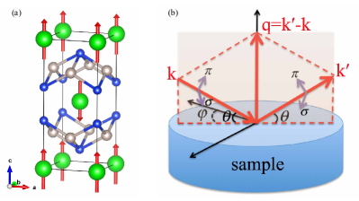
Figure 1: (Color online). (a) The crystal structure of URu₂Si₂. We assume a type-I antiferro-multipolar order on Uranium sites. (b) Illustration of experimental setup. A beam of polarized x-rays $\boldsymbol{k}$ is incident on the $[001]$ sample face with an angle $\theta$ and scattered by electrons, and then the scattered x-rays $\boldsymbol{k}^{\prime}$ with outgoing angle $\theta$ and specific polarization is analyzed. $\varphi$ is the azimuthal angle. For linear polarization, $\pi$ ($\sigma$) polarization is parallel (normal) to the scattering plane.

II methods

II.1 Atomic calculations

Fig. 1(a) is the crystal structure of URu₂Si₂, which has a body-centered tetragonal structure. In the present study, we assume a type-I antiferro-multipolar order on U sites, where sublattice A: U$(0,0,0)$ and sublattice B: U$(0.5,0.5,0.5)$ have opposite signs of the expectation value of the multipolar moment. The ordering wavevector is $Q_{\text{AF}}=(0,0,1)$. Fig. 1(b) is a typical experimental setup of REXS. A beam of polarized X-ray $\boldsymbol{k}$ is incident on the sample with an angle $\theta$ and then the scattered X-ray $\boldsymbol{k}^{\prime}$ with outgoing angle $\theta$ and specific polarization is analyzed. The double-differential cross section Ament et al. (2011) for REXS is,

$$\frac{\text{d}^{2}\sigma}{\text{d}\Omega\text{d}E}=r^{2}_{e}m^{2}\omega_{k^{\prime}}^{3}\omega_{k}\left|\mathcal{F}_{gg}\left(\boldsymbol{k},\boldsymbol{k}^{\prime},\hbar\omega_{k},\hbar\omega_{k^{\prime}},\boldsymbol{\epsilon},\boldsymbol{\epsilon}^{\prime}\right)\right|^{2},$$ (1)

where, $r_{e}=e^{2}/(4\pi\epsilon_{0}mc^{2})$ is the classical electron radius, $\mathcal{F}_{gg}$ is the scattering amplitude at zero temperature,

$$\mathcal{F}_{gg}\left(\boldsymbol{k},\boldsymbol{k}^{\prime},\hbar\omega_{k},\hbar\omega_{k^{\prime}},\boldsymbol{\epsilon},\boldsymbol{\epsilon}^{\prime}\right)=\sum_{n}\frac{\Braket{g}{\hat{\mathcal{D}}^{\prime\dagger}}{n}\Braket{n}{\hat{\mathcal{D}}}{g}}{\hbar\omega_{k}+E_{g}-E_{n}+i\Gamma/2},$$ (2)

where, $\boldsymbol{k}$ is the incoming light with energy $\hbar\omega_{k}$ and polarization $\boldsymbol{\epsilon}$, $\boldsymbol{k}^{\prime}$ is the outgoing light with energy $\hbar\omega_{k^{\prime}}$ and polarization $\boldsymbol{\epsilon}^{\prime}$, and $\boldsymbol{q}=\boldsymbol{k^{\prime}}-\boldsymbol{k}$ is the scattering vector. $\Ket{g},E_{g}$ is the ground state and $\Ket{n},E_{n}$ is the eigenstate of the intermediate Hamiltonian including a core-hole. $\Gamma$ is the lifetime width of the core hole. For U, $\Gamma\approx 8$ eV at the $L_{3}$ edge and $\Gamma\approx 3.5$ eV at the $M_{4}$ edge. $\hat{\mathcal{D}}$ and $\hat{\mathcal{D}}^{\prime\dagger}$ are the transition operators for absorption and emission processes,

$$\hat{\mathcal{D}} = \boldsymbol{P}^{(m)}\cdot\sum_{\boldsymbol{R}}\hat{\boldsymbol{D}}_{\boldsymbol{R}}^{(m)}$$ (3)

$$= \boldsymbol{P}^{(m)}\cdot\left(\sum_{\boldsymbol{R}}e^{i\boldsymbol{k}\cdot\boldsymbol{R}}\sum_{i}\hat{\boldsymbol{r}}_{\boldsymbol{R},i}^{(m)}\right),$$

$$\hat{\mathcal{D}}^{\prime\dagger} = \boldsymbol{P}^{(m)\prime\star}\cdot\sum_{\boldsymbol{R}}\hat{\boldsymbol{D}}_{\boldsymbol{R}}^{(m)\dagger}$$ (4)

$$= \boldsymbol{P}^{(m)\prime\star}\cdot\left(\sum_{\boldsymbol{R}}e^{-i\boldsymbol{k^{\prime}}\cdot\boldsymbol{R}}\sum_{i}\hat{\boldsymbol{r}}_{\boldsymbol{R},i}^{(m)\dagger}\right)$$

where, $\boldsymbol{R}$ is the site index, $i$ is the index of electron that is bound to site $\boldsymbol{R}$. $\boldsymbol{P}^{(m)}$ is a rank-$m$ tensor for geometry part including polarization and wavevector of photon, $\hat{\boldsymbol{r}}^{(m)}$ is a single particle rank-$m$ tensor operator of electron.

For E1-E1 transition,

$$\boldsymbol{P}^{(1)}\cdot\hat{\boldsymbol{r}}^{(1)} = \epsilon_{x}\hat{x}+\epsilon_{y}\hat{y}+\epsilon_{z}\hat{z},$$ (5)

$$\boldsymbol{P}^{(1)\prime\star}\cdot\hat{\boldsymbol{r}}^{(1)\dagger} = \epsilon_{x}^{\prime\star}\hat{x}+\epsilon_{y}^{\prime\star}\hat{y}+\epsilon_{z}^{\prime\star}\hat{z}.$$ (6)

For E2-E2 transition Nagao and Igarashi (2006),

$$(\hat{\boldsymbol{r}}^{(2)})_{1} = \frac{\sqrt{3}}{2}(\hat{x}^{2}-\hat{y}^{2}),$$ (7)

$$(\hat{\boldsymbol{r}}^{(2)})_{2} = \frac{1}{2}(3\hat{z}^{2}-\hat{r}^{2}),$$ (8)

$$(\hat{\boldsymbol{r}}^{(2)})_{3} = \sqrt{3}\hat{y}\hat{z},$$ (9)

$$(\hat{\boldsymbol{r}}^{(2)})_{4} = \sqrt{3}\hat{z}\hat{x},$$ (10)

$$(\hat{\boldsymbol{r}}^{(2)})_{5} = \sqrt{3}\hat{x}\hat{y},$$ (11)

and

$$\boldsymbol{P}^{(2)}_{1} = \frac{k}{3}\frac{\sqrt{3}}{2}(\epsilon_{x}\tilde{k}_{x}-\epsilon_{y}\tilde{k}_{y}),$$ (12)

$$\boldsymbol{P}^{(2)}_{2} = \frac{k}{3}\frac{1}{2}(2\epsilon_{z}\tilde{k}_{z}-\epsilon_{x}\tilde{k}_{x}-\epsilon_{y}\tilde{k}_{y}),$$ (13)

$$\boldsymbol{P}^{(2)}_{3} = \frac{k}{3}\frac{\sqrt{3}}{2}(\epsilon_{y}\tilde{k}_{z}+\epsilon_{z}\tilde{k}_{y}),$$ (14)

$$\boldsymbol{P}^{(2)}_{4} = \frac{k}{3}\frac{\sqrt{3}}{2}(\epsilon_{z}\tilde{k}_{x}+\epsilon_{x}\tilde{k}_{z}),$$ (15)

$$\boldsymbol{P}^{(2)}_{5} = \frac{k}{3}\frac{\sqrt{3}}{2}(\epsilon_{x}\tilde{k}_{y}+\epsilon_{y}\tilde{k}_{x}).$$ (16)

where, $k$ and $\tilde{\boldsymbol{k}}$ are the length and direction of the wavevector, respectively. We assume the absorption and emission process take place at the same site, then the scattering amplitude can be written as,

$$\mathcal{F}_{gg}\propto\sum_{\boldsymbol{R}}e^{-i\boldsymbol{q}\cdot\boldsymbol{R}}F_{gg}^{\boldsymbol{R}},$$ (17)

with

$$F_{gg}^{\boldsymbol{R}}=\sum_{n}\frac{\Braket{g}{\hat{\mathcal{D}}_{\boldsymbol{R}}^{\dagger}}{n}\Braket{n}{\hat{\mathcal{D}}_{\boldsymbol{R}}}{g}}{\hbar\omega_{\boldsymbol{k}}+E_{g}-E_{n}+i\Gamma/2}.$$ (18)

where $\hat{\mathcal{D}}_{\boldsymbol{R}}=\boldsymbol{P}^{(m)}\cdot\hat{\boldsymbol{D}}_{\boldsymbol{R}}^{(m)}$ and $\hat{\mathcal{D}}_{\boldsymbol{R}}^{\dagger}=\boldsymbol{P}^{(m)\prime\star}\cdot\hat{\boldsymbol{D}}_{\boldsymbol{R}}^{(m)\dagger}$.

We further make single atom approximation, i.e., approximating the states $\Ket{g}$ and $\Ket{n}$ as single atomic states. Then the total scattering amplitude can be written as the summation of the contributions from two sublattices A and B of U atoms,

$$\mathcal{F}_{gg}\propto\sum_{\boldsymbol{R}_{A}}e^{-i\boldsymbol{q}\cdot\boldsymbol{R}_{A}}F_{gg}^{\boldsymbol{R}_{A}}+\sum_{\boldsymbol{R}_{B}}e^{-i\boldsymbol{q}\cdot\boldsymbol{R}_{B}}F_{gg}^{\boldsymbol{R}_{B}},$$ (19)

where,

$$F^{\boldsymbol{R}_{A}}_{gg} = \sum_{n}\frac{\Braket{g^{A}}{\hat{\mathcal{D}}_{\boldsymbol{R}_{A}}^{\dagger}}{n^{A}}\Braket{n^{A}}{\hat{\mathcal{D}}_{\boldsymbol{R}_{A}}}{g^{A}}}{\hbar\omega_{k}+E_{g^{A}}-E_{n^{A}}+i\Gamma/2},$$ (20)

$$F^{\boldsymbol{R}_{B}}_{gg} = \sum_{n}\frac{\Braket{g^{B}}{\hat{\mathcal{D}}_{\boldsymbol{R}_{B}}^{\dagger}}{n^{B}}\Braket{n^{B}}{\hat{\mathcal{D}}_{\boldsymbol{R}_{B}}}{g^{B}}}{\hbar\omega_{k}+E_{g^{B}}-E_{n^{B}}+i\Gamma/2}.$$ (21)

$\Ket{g^{A}}(\Ket{n^{A}})$ and $\Ket{g^{B}}(\Ket{n^{B}})$ are the ground (intermediate) states of U atoms A and B, respectively. In calculation, we choose the ground states to induce opposite signs of the expectation value of multipolar moment at the A and B site.

We use the Cowan-Butler-Thole approach Cowan (1981); Butler (1981); Groot and Kotani (2008); Stavitski and de Groot (2010) to exactly diagonalize the atomic Hamiltonian for ground and excited configurations and then get the transition matrix. For URu₂Si₂, we assume a $5f^{2}$ ground configuration. For $M_{4}$-$E1$, $L_{3}$-$E1$ and $L_{3}$-$E2$ transitions, the excited configurations are $3d^{5}5f^{3}$, $2p^{5}5f^{2}6d^{1}$ and $2p^{5}5f^{3}$, respectively. The Slater integrals $F^{k},G^{k}$ and spin-orbit coupling (SOC) $\zeta$ of the valence and core electrons are calculated by the Hartree-Fock (HF) methods in Cowan’s code Cowan (1981). Usually, HF will overestimate them, so we rescale $F^{k},G^{k}$ by 80% and rescale SOC $\zeta$ by 92% for $2p$ core hole and 96% for $3d$ core hole, respectively. The parameters are listed in the Appendix.

According to Hund’s rule coupling, the $5f^{2}$ configuration has a ground state with total angular momentum $J=4$ under $SO(3)$ symmetry. With $D_{4h}$ crystalline electric field (CEF) symmetry, these nine ground state will split into five singlets and two doublets Kusunose and Harima (2011); Sundermann et al. (2016),

$$\Ket{A_{1g}^{(1)}(\alpha)} = \text{cos}\alpha\Ket{0}+\frac{\text{sin}\alpha}{\sqrt{2}}\left(\Ket{4}+\Ket{-4}\right),$$ (22)

$$\Ket{A_{1g}^{(2)}(\alpha)} = \text{sin}\alpha\Ket{0}-\frac{\text{cos}\alpha}{\sqrt{2}}\left(\Ket{4}+\Ket{-4}\right),$$ (23)

$$\Ket{A_{2g}} = \frac{i}{\sqrt{2}}\left(\Ket{4}-\Ket{-4}\right),$$ (24)

$$\Ket{B_{1g}} = \frac{1}{\sqrt{2}}\left(\Ket{2}+\Ket{-2}\right),$$ (25)

$$\Ket{B_{2g}} = \frac{i}{\sqrt{2}}\left(\Ket{2}-\Ket{-2}\right),$$ (26)

$$\Ket{E_{g}^{(1)}(\beta)} = \text{cos}\beta\Ket{\mp 1}+\text{sin}\beta\Ket{\pm 3},$$ (27)

$$\Ket{E_{g}^{(2)}(\beta)} = \text{sin}\beta\Ket{\mp 1}-\text{cos}\beta\Ket{\pm 3}.$$ (28)

In Ref. Kusunose and Harima (2011), the authors list the definition of the multipole up to rank-5. We will follow this definition in the present paper and only discuss multipole up to rank-4 that can, in principle, be detected via the $E2$ transition. We build different ground states which will induce dipole, quadrupole, octupole and hexadecapole orders.

The ground state that will induce $A_{2+}(A_{2-})$ order can be constructed by a linear combination of $\Ket{A_{2g}}$ and $\Ket{A_{1g}^{(2)}}$,

$$\Ket{g^{A(B)}}=\frac{1}{\sqrt{2}}\left(\Ket{A_{2g}}\pm e^{i\eta}\Ket{A_{1g}^{(2)}(40^{o})}\right),$$ (29)

where, we take plus sign for $\Ket{g^{A}}$ and minus sign for $\Ket{g^{B}}$. Note that the subscript $+(-)$ in $A_{2+}(A_{2-})$ means time-reversal even (odd). When $\eta=0$, it will induce a $A_{2+}$ hexadecapolar order $H_{z}^{\alpha}=\frac{\sqrt{35}}{2}\overline{J_{x}J_{y}(J_{x}^{2}-J_{y}^{2})}$, while $\eta=\pi/2$, it will induce a $A_{2-}$ dipolar order $J_{z}$ and octupolar order $T_{z}^{\alpha}=\frac{1}{2}\overline{J_{z}(5J_{z}^{2}-3J^{2})}$. This scheme is proposed by Haule and Kotliar Haule and Kotliar (2009) by a LDA+DMFT calculation. In their LDA+DMFT calculation, they also figure out $\alpha$ in $A_{1g}^{(2)}$ should be about $40^{\circ}$. $H_{z}^{\alpha}$ is proposed to be the primary OP in the HO phase. It can be also induced as a secondary OP in the hastatic order scheme Chandra et al. (2015).

The ground state that will induce $B_{1+}(B_{1-})$ order can be written as,

$$\Ket{g^{A(B)}}=\frac{1}{\sqrt{2}}\left(\Ket{B_{1g}}\pm e^{i\eta}\Ket{A_{1g}^{(2)}(40^{o})}\right),$$ (30)

When $\eta=0$, it will induce a $B_{1+}$ quadrupolar order Ohkawa and Shimizu (1999) $O_{22}=\frac{\sqrt{3}}{2}\overline{J_{x}^{2}-J_{y}^{2}}$ and hexadecapolar order $O_{42}=\frac{\sqrt{5}}{4}\overline{(J_{x}^{2}-J_{y}^{2})(7J_{z}^{2}-J^{2})}$, while $\eta=\pi/2$ it will induce a $B_{1-}$ octupolar order Kiss and Fazekas (2005) $T_{xyz}=\sqrt{15}\overline{J_{x}J_{y}J_{z}}$.

The ground state that will induce $B_{2+}(B_{2-})$ order can be written as,

$$\Ket{g^{A(B)}}=\frac{1}{\sqrt{2}}\left(\Ket{B_{2g}}\pm e^{i\eta}\Ket{A_{1g}^{(2)}(40^{o})}\right),$$ (31)

when $\eta=0$ it will induce a $B_{2+}$ quadrupolar order Ohkawa and Shimizu (1999) $O_{xy}=\sqrt{3}\overline{J_{x}J_{y}}$ and hexadecapolar order $H_{z}^{\beta}=\frac{\sqrt{5}}{2}\overline{J_{x}J_{y}(7J_{z}^{2}-J^{2})}$, while $\eta=\pi/2$, it will induce a $B_{2-}$ octupolar order Kiss and Fazekas (2005) $T_{z}^{\beta}=\frac{\sqrt{15}}{2}\overline{J_{z}(J_{x}^{2}-J_{y}^{2})}$.

II.2 REXS Experiment

URu₂Si₂ samples were grown using the Czocharalski method D. Matsuda et al. (2008). The residual resistivity ratio (RRR) was measured in various pieces of sample; the REXS experiment was performed on the sample with highest RRR (= 361). REXS measurements were performed across the U $L_{3}$ edge ($\approx$ 17.21 keV) at the 6-ID-B beamline of the Advanced Photon Source at Argonne National Laboratory. The sample was glued to a Cu holder using GE varnish. The holder was placed inside a Be dome filled with He gas, which in turn was mounted on the cold finger of a He closed cycle cryostat. A six circle diffractometer was used to move through reciprocal space. Measurements were performed using a scintillator point detector with $1\times 1$ mm² slits. Tetragonal notation with $a=b=4.108$ Å and $c=9.514$ Å is used throughout the paper.

III results and discussion

III.1 Azimuthal dependence for different multipolar order parameters

In REXS experiment, azimuthal measurements are used to identify the symmetry of the underlying OPs. Although Nagao et al. Nagao and Igarashi (2006) have figured out the analytic formula of the azimuthal dependences for $E2$ transition, we still explicitly calculate and plot the azimuthal dependences to show the symmetry difference for different multipolar OPs. The results for a $(0,0,3)$ reflection are plotted in Fig. 2. For each multipolar OP, both $\sigma\pi$ and $\sigma\sigma$ channels are plotted, and their intensity is normalized by the maximum of the $\sigma\pi$ channel. Fig. 2(a,b) plots the results of the $A_{2+}$ hexadecapole $H_{z}^{\alpha}$. It shows an eight-fold symmetry with a $\pi/8$ phase shift between the $\sigma\pi$ and $\sigma\sigma$ channels. The peak intensity of the $\sigma\sigma$ channel is about 2 orders of magnitude larger than that of the $\sigma\pi$ channel. The eight-fold symmetry is a characteristic of this $H_{z}^{\alpha}$ hexadecapolar OP. Fig. 2(c,d) shows the results of the $A_{2-}$ dipole $J_{z}$ and octupole $T_{z}^{\alpha}$. It shows a nonzero constant in the $\sigma\pi$ channel and no signal in the $\sigma\sigma$ channel. Fig. 2(e,f) displays the results of the $B_{1+}$ quadrupole $O_{22}$ and hexadecapole $O_{42}$. It shows a $d_{xy}$ wave pattern in the $\sigma\pi$ channel and $d_{x^{2}-y^{2}}$ wave pattern in the $\sigma\sigma$ channel. In Fig. 2(g,h) the results of $B_{1-}$ octupole $T_{xyz}$ shows a $d_{xy}$ wave pattern in the $\sigma\pi$ channel and no signal in the $\sigma\sigma$ channel. Fig. 2(i,j) plots the results of $B_{2+}$ quadrupole $O_{xy}$ and hexadecapole $H_{z}^{\beta}$ exhibiting a $d_{x^{2}-y^{2}}$ wave pattern in the $\sigma\pi$ channel and $d_{xy}$ pattern in the $\sigma\sigma$ channel. Finally, the results of the $B_{2-}$ octupole $T_{z}^{\beta}$ are shown in Fig. 2(k,l) where a $d_{x^{2}-y^{2}}$ wave pattern is seen in the $\sigma\pi$ channel and nothing is seen in the $\sigma\sigma$ channel. In general, we find that there are no signals in $\sigma\sigma$ channel for time-reversal broken OPs. The azimuthal dependence show different symmetries for different multipole, so it can be used to distinguish multipolar OPs.

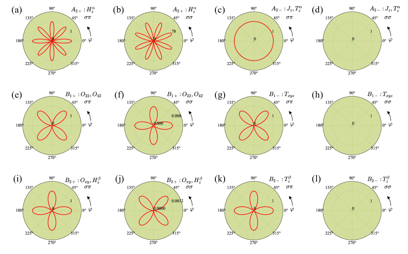
Figure 2: (Color online). The calculated azimuthal dependence of a $(0,0,3)$ reflection of $L_{3}$-$E2$ transition in both $\sigma\pi$ and $\sigma\sigma$ channels for different proposals of multipolar OPs. The incident photon energy is 17.167 keV and the azimuthal angle is defined with respect to $[100]$ direction. For each proposal, the intensity is normalized by the maximum intensity of its $\sigma\pi$ channel. (a,b) $A_{2+}$ hexadecapole $H_{z}^{\alpha}$, (c,d) $A_{2-}$ dipole $J_{z}$ and ocutpole $T_{z}^{\alpha}$, (e,f) $B_{1+}$ quadrupole $O_{22}$ and hexadecapole $O_{42}$, (g,h) $B_{1-}$ octupole $T_{xyz}$, (i,j) $B_{2+}$ quadrupole $O_{xy}$ and hexadecapole $H_{z}^{\beta}$, (k,l) $B_{2-}$ octupole $T_{z}^{\beta}$.

III.2 REXS Results

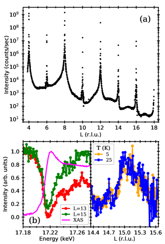
Figure 3: (a) X-ray diffraction $L$ dependence measured along $(0,0,L)$ direction using 17.215 keV and $\varphi=1.2^{\circ}$. (b) Energy dependence of (0,0,13) and (0,0,15) Bragg peaks together with the U $L_{3}$ edge XANES. (c) Temperature dependence of (0,0,15) Bragg peak.

The body centered tetragonal structure of $\mathrm{URu_{2}Si_{2}}$ forbids Bragg peaks with $H+K+L=2n+1$. We infer that the HO state breaks the body centered symmetry by creating inequivalent U sites, thus allowing Bragg peaks at these once forbidden positions. We performed an extensive search for HO Bragg peaks along $(0,0,L)$ and $(1,0,L)$ directions; results for the former are displayed in Fig. 3. Broad peaks are observed at $(0,0,2n+1)$. However, these peaks persist through the phase transition at $T_{HO}$, strongly suggesting that these are not related to the HO phase. Additionally, no resonance enhancement is observed across the U $L_{3}$ edge. This suggests that the HO is not accessible through the $E1$ or $E2$ transitions using experiments of this type. These results are consistent with former studies Amitsuka et al. (2010); Walker et al. (2011) in which no quadrupolar OPs are found. However, we still cannot exclude the possibility of octupole and hexadecapole due to the weak signal of the $E2$ transition.

Despite our negative result in the search for the HO, additional experiments are needed to definitely prove the existence (or absence) of the octupole or hexadecapole OPs. Designing experimental techniques to enhance the sensitivity to the $E2$ transition at U-$L_{3}$ edge is needed to observe higher rank multipoles. One of such techniques is the Borrmann spectroscopy Batterman and Cole (1964); Pettifer et al. (2008). The Borrmann effect refers to the anomalous transmission of X-rays through very perfect single-crystal slabs when they are in symmetric Laue diffraction condition Batterman and Cole (1964). This effect can be interpreted by the theory of dynamical diffraction of X-rays Batterman and Cole (1964). It is a consequence of multiple coherent interference of the incident and diffracted beams which produces a total electric field with almost zero amplitude but largely enhanced gradient at the crystal planes. The dipolar transition is thus suppressed because it is proportional to the amplitude of the electric field and, on the contrary, the quadrupolar transition will be largely enhanced because it is proportional to the gradient of the electric field. Therefore, we may have a chance to detect strong quadrupolar signal, for example at U-$L_{3}$ edge. In Ref. Pettifer et al., 2008, Pettifer et al. indeed observed very strong quadrupolar peak in the absorption spectrum at $L_{1}$, $L_{2}$ and $L_{3}$ edges of Gadolinium in a $4f$ compound gadolinium gallium garnet. However, no results of $5f$ compounds have been reported, so it is worth to try in $5f$ compounds, such as URu₂Si₂. Borrmann spectroscopy requires samples that are much thicker than the nominal X-ray penetration depth and sufficiently perfect that at least some x-rays can transmit through the sample without encountering defects, which may be a challenge for sample growth.

Polarization analysis of the outgoing X-rays can also be advantageous (despite the strong reduction in X-ray throughput that it imposes) because, as we will demonstrate, the HO Bragg peak should be observed in the $\sigma\pi$ channel. Additionally, identifying the energy and cross-section of the $L_{3}$- $E2$ transition will greatly facilitate the search for superlattice peaks.

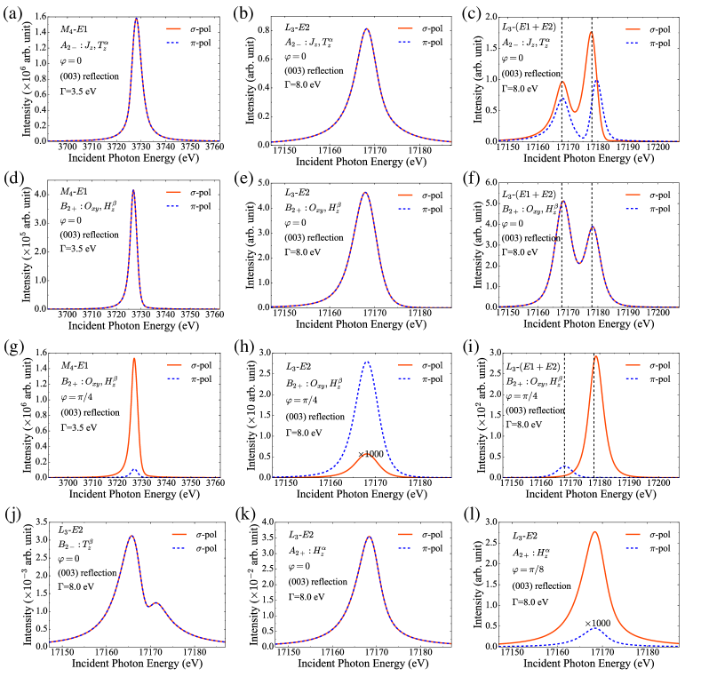
Figure 4: (Color online). $(0,0,3)$ REXS intensity as a function of incident photon energy and polarization. The incoming light is linearly polarized and the polarization of the outgoing light is not analyzed. We compare the results of the $M_{4}$-$E1$ transition with the $L_{3}$-$E2$ transition and the $L_{3}$-($E1$ + $E2$) transition. We consider different ordering schemes: (a,b,c) Antiferro-dipole $J_{z}$ and antiferro-octupole $T_{z}^{\alpha}$ at $\varphi=0$. (d,e,f) Antiferro-quadrupole $O_{xy}$ and antiferro-hexadecapole $H_{z}^{\beta}$ at $\varphi=0$. (g,h,i) Antiferro-quadrupole $O_{xy}$ and antiferro-hexadecapole $H_{z}^{\beta}$ at $\varphi=\frac{\pi}{4}$. (j) Antiferro-octupole $T_{z}^{\beta}$ at $\varphi=0$. (k) Antiferro-hexadecapole $H_{z}^{\alpha}$ at $\varphi=0$. (l) Antiferro-hexadecapole $H_{z}^{\alpha}$ at $\varphi=\pi/8$.

III.3 Intensity estimation of the $L_{3}$-$E2$ transition

We further justify the negative experimental results by estimating the intensity of the $L_{3}$-$E2$ transition. Usually, the intensity of the $E2$ transition will be much weaker than that of the $E1$ transition. This is mainly caused by the very small overlap integral of $r^{2}$ between the core hole and valence orbitals. Thus, it is critical to give an estimation of the relative intensity of the $L_{3}$-$E2$ transition compared with known experiments which have strong intensity, such as the $M_{4}$-$E1$ transition. Roughly, the relative intensity between $L_{3}$-$E2$ and $M_{4}$-$E1$ is,

$$\frac{I(L_{3}-E2)}{I(M_{4}-E1)}\propto\left(\frac{k}{3}\frac{\omega_{L_{3}}}{\omega_{M_{4}}}\frac{\Braket{2p}{r^{2}}{5f}}{\Braket{3d}{r}{5f}}\right)^{4}\left(\frac{\Gamma_{M_{4}}}{\Gamma_{L_{3}}}\right)^{2},$$ (32)

and that between $L_{3}$-$E2$ and $L_{3}$-$E1$ is,

$$\frac{I(L_{3}-E2)}{I(L_{3}-E1)}\propto\left(\frac{k}{3}\frac{\Braket{2p}{r^{2}}{5f}}{\Braket{2p}{r}{6d}}\right)^{4},$$ (33)

where, $\omega_{L_{3}}$ and $\omega_{M_{4}}$ are the X-ray frequency of the $L_{3}$ and $M_{4}$ edges, their ratio is about 4.6. Based on the HF calculations, the overlap integral ratio $\Braket{2p}{r^{2}}{5f}/\Braket{3d}{r}{5f}\approx 0.013$ and $\Braket{2p}{r^{2}}{5f}/\Braket{2p}{r}{6d}\approx 0.2$, respectively. $\Gamma_{M_{4}}$ and $\Gamma_{L_{3}}$ are the core-hole lifetime width for $M_{4}$ and $L_{3}$ edge, respectively, and their ratio is $\Gamma_{M_{4}}/\Gamma_{L_{3}}\approx 0.4$. For the $L_{3}$ edge, $k/3\approx 2.9$. Thus, the intensity of $L_{3}$-$E2$ is about $10^{-4}$ times smaller than that of $M_{4}$-$E1$ and $10^{-1}$ times smaller than that of $L_{3}$-$E1$. Here, we should note that $6d$ orbitals are much broader in URu₂Si₂, which will lead to larger overlap integrals than those based on the atomic $6d$ orbitals, so $L_{3}$-$E2$ is not just one order of magnitude smaller than that of $L_{3}$-$E1$. We may expect larger overlap integrals for the $M_{3}$-$E2$ ($3p_{3/2}\rightarrow 5f$) transition, so we also calculate the relative intensity between $M_{3}$-$E2$ and $M_{4}$-$E1$. The results show that the intensity of $M_{3}$-$E2$ is also about $10^{-4}$ times smaller than that of $M_{4}$-$E1$. The reason is that, although the calculated overlap integral $\Braket{3p}{r^{2}}{5f}$ is about 14 times larger than that of $\Braket{2p}{r^{2}}{5f}$, both of the X-ray frequency and wavevector of $M_{3}$ edge is about 0.25 times smaller than that of $L_{3}$ edge, as a result, the enhancement effect from the larger overlap integral is cancelled out. The intensity of $M_{3}$-$E2$ is not stronger than that of $L_{3}$-$E2$.

However, this rough estimation does not consider many details of the scattering process, such as the ground state and the intermediate excited states, the interference effects of intermediate states, the smearing effect of core-hole lifetime width and the geometry of the experimental setup. To give a better estimation, we exactly diagonalize the atomic ground and excited Hamiltonians to get the eigenstates and the transition matrix, and then we choose different ground states and experimental geometries to calculate the cross section according to Eqn. 1 and Eqn. 2.

The calculated results of a $(0,0,3)$ reflection are shown in Fig. 4. The azimuthal angle $\varphi$ is defined with respect to the $[100]$ direction and the polarization of outgoing light is not analyzed. We plot both the $\sigma$ and $\pi$ polarizations of the incident light. The difference of energy levels between $6d$ and $5f$ is set to be 10 eV. We assume a type-I antiferro-multipolar order with $Q_{AF}=(0,0,1)$ in the simulation. Fig. 4(a,b,c) are the results for the ground state (Eqn. 29) that induces $A_{2-}$ orders: dipole $J_{z}$ and octupole $T_{z}^{\alpha}$. The $E1$ transition can only detect $J_{z}$ but $E2$ can detect both of them. The azimuthal angle is set to be $\varphi=0$. For this ground state, the intensity of $L_{3}$-$E2$ is about $10^{-6}$ times smaller than that of $M_{4}$-$E1$. However, the intensity of $L_{3}$-$E2$ is almost the same order of magnitude as that of $L_{3}$-$E1$ transition. In Fig. 4(c), the left peak is from the $E2$ transition and the right peak is from the $E1$ transition. Fig. 4(d,e,f,g,h,i) plots the results for the ground state (Eqn. 31) that induces $B_{2+}$ order: quadrupole $O_{xy}$ and hexadecapole $H_{z}^{\beta}$. In Fig. 4(d,e,f) the azimuthal angle is $\varphi=0$. We find that the intensity of $L_{3}$-$E2$ transition is $10^{-5}$ times smaller than that of $M_{4}$-$E1$ transition and has the same order of magnitude as that of $L_{3}$-$E1$. In Fig. 4(g,h,i), the azimuthal angle is set to be $\varphi=\pi/4$. For $\sigma$ polarization, the intensity of $L_{3}$-$E2$ is about $10^{-9}$ times smaller than that of $M_{4}$-$E1$ and $10^{-5}$ smaller than that of $L_{3}$-$E1$. However, for $\pi$ polarization, it is only $10^{-5}$ times smaller than that of $M_{4}$-$E1$ and much larger than that of $L_{3}$-$E1$ so that there is only a $E2$ peak. Fig. 4(j) is the result for the ground state (Eqn. 31) that induces $B_{2-}$ octupolar order $T_{z}^{\beta}$. The intensity is at least 8 order of magnitude smaller than that of $M_{4}$-$E1$. Another $B_{1-}$ octupole $T_{xyz}$ has the same order of magnitude as that of $T_{z}^{\beta}$. Fig. 4(k,l) are the results for the ground state (Eqn. 29) that induces the $A_{2+}$ hexadecapolar order $H_{z}^{\alpha}$. For $\varphi=0$, both $\sigma$ and $\pi$ polarizations are at least 7 order of magnitude smaller than that of $M_{4}$-$E1$. For $\varphi=\pi/8$, $\sigma$ polarization is about 5 order of magnitude smaller than that of $M_{4}$-$E1$. We emphasize that the atomic calculation underestimate the intensity of $L_{3}$-$E1$ transition due to the itinerant character of $6d$ orbitals, so the intensity of $L_{3}$-$E1$ should be much larger than that of $L_{3}$-$E2$ in reality.

Based on these atomic results, we find that there are many factors that will affect the REXS cross-section, such as the interference of the intermediate states, the interference effect of core-hole lifetime width, the experimental geometry and the details of the ground states. Overall, the intensity of $L_{3}$-$E2$ transition is at least 5 or 6 orders of magnitude smaller than that of $M_{4}$-$E1$, so the signal of $L_{3}$-$E2$ transition is indeed very weak compared with $M_{4}$-$E1$. We also note that the $5f$ electrons are not completely localized and they have partial itinerant character in URu₂Si₂, which leads to the importance of the band effects in the REXS cross-section. To account for these effects, the combination of more advanced first-principle calculations, such as density functional theory plus dynamical mean-field theory (DFT+DMFT), with REXS cross-section calculations is needed. Despite this, the simple atomic simulations still give us preliminary estimations about the strength of the $E2$ transition.

To further confirm the weakness of $L_{3}$-$E2$ signal, we estimate the flux of the scattered photons by calculating the absolute value of the cross-section. For a typical flux of $10^{11}\text{ph}/\text{s}/100\text{meV}/(100\times 100\mu m^{2})$, a rough upper bound of the flux of scattered photon is $10^{4}\text{ph}/\text{s}/\text{eV}/\text{rad}$ for $M_{4}$-$E1$ transition, while it is $10^{-1}\sim 10^{-2}\text{ph}/\text{s}/\text{eV}/\text{rad}$ for $L_{3}$-$E2$ transition. This makes it very difficult to be detected in experiments, which is consistent with the experimental results.

IV summary

In summary, we have studied the possibility to detect multipolar OPs in URu₂Si₂ by REXS in the U $L_{3}$-$E2$ transition channel. The REXS experiments do not find any clear signal indicating multipolar OPs. An estimation based on atomic calculations indicates that the intensity of the $L_{3}$-$E2$ transition is indeed much smaller than that of $M_{4}$-$E1$ transition and the flux of the scattered photons is too small such that it is very difficult to detect the $E2$ signal. It seems that it is still not practical to use the $E2$ transition of currently available REXS experiment to detect the multipolar OPs. Developing experimental techniques to enhance $E2$ signal is urgently needed to identify the multipolar OPs not only in URu₂Si₂ but also in other compounds, such as UO₂, NpO₂ and Ce_1-xLa_xB₆ Santini et al. (2009).

V acknowledgments

We thank Frank de Groot for valuable discussions. This work was supported by the U.S. Department of energy, Office of Science, Basic Energy Sciences as a part of the Computational Materials Science Program through the Center for Computational Design of Functional Strongly Correlated Materials and Theoretical Spectroscopy. G.F. and D.M. were supported by the U.S. Department of Energy, Office of Science, Office of Basic Energy Sciences, under Contract No. DE-SC00112704, and Early Career Award Program under Award No. 1047478. X.L. is supported by MOST (Grant No.2015CB921302) and CAS (Grant No. XDB07020200). This research used resources of the Advanced Photon Source, a U.S. Department of Energy (DOE) Office of Science User Facility operated for the DOE Office of Science by Argonne National Laboratory under Contract No. DE-AC02-06CH11357. Work at Los Alamos National Laboratory was performed under the auspices of the U.S. Department of Energy, Office of Basic Energy Sciences, Division of Materials Sciences and Engineering.

Appendix A Slater integrals and spin-orbit coupling parameters

Table 1: Slater integrals and spin-orbit coupling parameters for ground configuration $5f^{2}$ (in eV).

$F^{0}_{ff}$	$F^{2}_{ff}$	$F^{4}_{ff}$	$F^{6}_{ff}$	$\zeta_{5f}$
0.291	7.611	4.979	3.655	0.261

Table 2: Slater integrals and spin-orbit coupling parameters for excited configuration $2p^{5}5f^{3}$ (in eV).

$F^{0}_{ff}$	$F^{2}_{ff}$	$F^{4}_{ff}$	$F^{6}_{ff}$	$F^{0}_{pf}$	$F^{2}_{pf}$	$G^{2}_{pf}$	$G^{4}_{pf}$
0.306	7.984	5.232	3.845	0.005	0.497	0.082	0.053
$\zeta_{5f}$	$\zeta_{2p}$
0.302	2517.292

Table 3: Slater integrals and spin-orbit coupling parameters for excited configuration $2p^{5}5f^{2}6d^{1}$ (in eV).

$F^{0}_{ff}$	$F^{2}_{ff}$	$F^{4}_{ff}$	$F^{6}_{ff}$	$F^{0}_{pf}$	$F^{2}_{pf}$	$G^{2}_{pf}$	$G^{4}_{pf}$
0.307	8.278	5.447	4.011	0.102	0.528	0.087	0.056
$F^{0}_{pd}$	$F^{2}_{pd}$	$G^{1}_{pd}$	$G^{3}_{pd}$	$F^{0}_{fd}$	$F^{2}_{fd}$	$F^{4}_{fd}$	$G^{1}_{fd}$
0.022	0.272	0.238	0.142	0.139	3.750	2.050	1.938
$G^{3}_{fd}$	$G^{5}_{fd}$	$\zeta_{5f}$	$\zeta_{6d}$	$\zeta_{2p}$
1.562	1.213	0.321	0.435	2517.236

Table 4: Slater integrals and spin-orbit coupling parameters for excited configuration $3d^{5}5f^{3}$ (in eV).

$F^{0}_{ff}$	$F^{2}_{ff}$	$F^{4}_{ff}$	$F^{6}_{ff}$	$F^{0}_{df}$	$F^{2}_{df}$	$F^{4}_{df}$
0.307	8.020	5.258	3.865	0.102	2.051	0.952
$G^{1}_{df}$	$G^{3}_{df}$	$G^{5}_{df}$	$\zeta_{5f}$	$\zeta_{3d}$
1.602	0.969	0.678	0.301	70.449

References

- Palstra et al. (1985) T. T. M. Palstra, A. A. Menovsky, J. v. d. Berg, A. J. Dirkmaat, P. H. Kes, G. J. Nieuwenhuys, and J. A. Mydosh, Phys. Rev. Lett. 55, 2727 (1985).
- Broholm et al. (1987) C. Broholm, J. K. Kjems, W. J. L. Buyers, P. Matthews, T. T. M. Palstra, A. A. Menovsky, and J. A. Mydosh, Phys. Rev. Lett. 58, 1467 (1987).
- Broholm et al. (1991) C. Broholm, H. Lin, P. T. Matthews, T. E. Mason, W. J. L. Buyers, M. F. Collins, A. A. Menovsky, J. A. Mydosh, and J. K. Kjems, Phys. Rev. B 43, 12809 (1991).
- MacLaughlin et al. (1988) D. E. MacLaughlin, D. W. Cooke, R. H. Heffner, R. L. Hutson, M. W. McElfresh, M. E. Schillaci, H. D. Rempp, J. L. Smith, J. O. Willis, E. Zirngiebl, C. Boekema, R. L. Lichti, and J. Oostens, Phys. Rev. B 37, 3153 (1988).
- Amitsuka et al. (2007) H. Amitsuka, K. Matsuda, I. Kawasaki, K. Tenya, M. Yokoyama, C. Sekine, N. Tateiwa, T. Kobayashi, S. Kawarazaki, and H. Yoshizawa, Journal of Magnetism and Magnetic Materials 310, 214 (2007).
- Amitsuka et al. (1999) H. Amitsuka, M. Sato, N. Metoki, M. Yokoyama, K. Kuwahara, T. Sakakibara, H. Morimoto, S. Kawarazaki, Y. Miyako, and J. A. Mydosh, Phys. Rev. Lett. 83, 5114 (1999).
- Butch et al. (2010) N. P. Butch, J. R. Jeffries, S. Chi, J. B. Leão, J. W. Lynn, and M. B. Maple, Phys. Rev. B 82, 060408 (2010).
- Santini and Amoretti (1994) P. Santini and G. Amoretti, Phys. Rev. Lett. 73, 1027 (1994).
- Santini (1998) P. Santini, Phys. Rev. B 57, 5191 (1998).
- Ohkawa and Shimizu (1999) F. J. Ohkawa and H. Shimizu, Journal of Physics: Condensed Matter 11, L519 (1999).
- Santini et al. (2000) P. Santini, G. Amoretti, R. Caciuffo, F. Bourdarot, and B. Fåk, Phys. Rev. Lett. 85, 654 (2000).
- Kiss and Fazekas (2005) A. Kiss and P. Fazekas, Phys. Rev. B 71, 054415 (2005).
- Hanzawa (2007) K. Hanzawa, Journal of Physics: Condensed Matter 19, 072202 (2007).
- Haule and Kotliar (2009) K. Haule and G. Kotliar, Nat. Phys. 5, 796 (2009).
- Cricchio et al. (2009) F. Cricchio, F. Bultmark, O. Grånäs, and L. Nordström, Phys. Rev. Lett. 103, 107202 (2009).
- Harima et al. (2010) H. Harima, K. Miyake, and J. Flouquet, Journal of the Physical Society of Japan 79, 033705 (2010).
- Kusunose and Harima (2011) H. Kusunose and H. Harima, Journal of the Physical Society of Japan 80, 084702 (2011).
- Ikeda et al. (2012) H. Ikeda, M. Suzuki, R. Arita, T. Takimoto, T. Shibauchi, and Y. Matsuda, Nat. Phys. 8, 528 (2012).
- Maple et al. (1986) M. B. Maple, J. W. Chen, Y. Dalichaouch, T. Kohara, C. Rossel, M. S. Torikachvili, M. W. McElfresh, and J. D. Thompson, Phys. Rev. Lett. 56, 185 (1986).
- Ikeda and Ohashi (1998) H. Ikeda and Y. Ohashi, Phys. Rev. Lett. 81, 3723 (1998).
- Mineev and Zhitomirsky (2005) V. P. Mineev and M. E. Zhitomirsky, Phys. Rev. B 72, 014432 (2005).
- Rau and Kee (2012) J. G. Rau and H.-Y. Kee, Phys. Rev. B 85, 245112 (2012).
- Gor’kov and Sokol (1992) L. P. Gor’kov and A. Sokol, Phys. Rev. Lett. 69, 2586 (1992).
- Chandra et al. (2002) P. Chandra, P. Coleman, J. A. Mydosh, and V. Tripathi, Nature 417, 831 (2002).
- Varma and Zhu (2006) C. M. Varma and L. Zhu, Phys. Rev. Lett. 96, 036405 (2006).
- Elgazzar et al. (2009) S. Elgazzar, J. Rusz, M. Amft, P. M. Oppeneer, and J. A. Mydosh, Nat Mater 8, 337 (2009).
- Fujimoto (2011) S. Fujimoto, Phys. Rev. Lett. 106, 196407 (2011).
- Dubi and Balatsky (2011) Y. Dubi and A. V. Balatsky, Phys. Rev. Lett. 106, 086401 (2011).
- Chandra et al. (2013) P. Chandra, P. Coleman, and R. Flint, Nature 493, 621 (2013).
- Chandra et al. (2015) P. Chandra, P. Coleman, and R. Flint, Phys. Rev. B 91, 205103 (2015).
- Mydosh and Oppeneer (2011) J. A. Mydosh and P. M. Oppeneer, Rev. Mod. Phys. 83, 1301 (2011).
- Mydosh and Oppeneer (2014) J. Mydosh and P. Oppeneer, Philosophical Magazine 94, 3642 (2014).
- Buhot et al. (2014) J. Buhot, M.-A. Méasson, Y. Gallais, M. Cazayous, A. Sacuto, G. Lapertot, and D. Aoki, Phys. Rev. Lett. 113, 266405 (2014).
- Kung et al. (2015) H.-H. Kung, R. E. Baumbach, E. D. Bauer, V. K. Thorsmølle, W.-L. Zhang, K. Haule, J. A. Mydosh, and G. Blumberg, Science 347, 1339 (2015), http://science.sciencemag.org/content/347/6228/1339.full.pdf .
- Kung et al. (2016) H.-H. Kung, S. Ran, N. Kanchanavatee, V. Krapivin, A. Lee, J. A. Mydosh, K. Haule, M. B. Maple, and G. Blumberg, Phys. Rev. Lett. 117, 227601 (2016).
- Ament et al. (2011) L. J. P. Ament, M. van Veenendaal, T. P. Devereaux, J. P. Hill, and J. van den Brink, Reviews of Modern Physics 83, 705 (2011).
- Matsumura et al. (2013) T. Matsumura, H. Nakao, and Y. Murakami, Journal of the Physical Society of Japan 82, 021007 (2013).
- Isaacs et al. (1990) E. D. Isaacs, D. B. McWhan, R. N. Kleiman, D. J. Bishop, G. E. Ice, P. Zschack, B. D. Gaulin, T. E. Mason, J. D. Garrett, and W. J. L. Buyers, Phys. Rev. Lett. 65, 3185 (1990).
- Nagao and ichi Igarashi (2005) T. Nagao and J. ichi Igarashi, Journal of the Physical Society of Japan 74, 765 (2005).
- Amitsuka et al. (2010) H. Amitsuka, T. Inami, M. Yokoyama, S. Takayama, Y. Ikeda, I. Kawasaki, Y. Homma, H. Hidaka, and T. Yanagisawa, Journal of Physics: Conference Series 200, 012007 (2010).
- Walker et al. (2011) H. C. Walker, R. Caciuffo, D. Aoki, F. Bourdarot, G. H. Lander, and J. Flouquet, Phys. Rev. B 83, 193102 (2011).
- dos Reis et al. (2016) R. D. dos Reis, L. S. I. Veiga, D. Haskel, J. C. Lang, Y. Joly, F. G. Gandra, and N. M. Souza-Neto, (2016), arXiv:1601.02443 [cond-mat.str-el] .
- Nagao and Igarashi (2006) T. Nagao and J.-i. Igarashi, Phys. Rev. B 74, 104404 (2006).
- Cowan (1981) R. D. Cowan, The Theory of Atomic Structure and Spectra (University of California Press, Berkeley, 1981).
- Butler (1981) P. H. Butler, Point Group Symmetry Applications: Methods and Tables (Plenum Press, New York, 1981).
- Groot and Kotani (2008) F. D. Groot and A. Kotani, Core level spectroscopy of solids (CRC press, 2008).
- Stavitski and de Groot (2010) E. Stavitski and F. M. de Groot, Micron 41, 687 (2010).
- Sundermann et al. (2016) M. Sundermann, M. W. Haverkort, S. Agrestini, A. Al-Zein, M. Moretti Sala, Y. Huang, M. Golden, A. de Visser, P. Thalmeier, L. H. Tjeng, and A. Severing, Proceedings of the National Academy of Sciences (2016), 10.1073/pnas.1612791113.
- D. Matsuda et al. (2008) T. D. Matsuda, D. Aoki, S. Ikeda, E. Yamamoto, Y. Haga, H. Ohkuni, R. Settai, and Y. Onuki, J. Phys. Soc. Japan 77, 362 (2008).
- Batterman and Cole (1964) B. W. Batterman and H. Cole, Rev. Mod. Phys. 36, 681 (1964).
- Pettifer et al. (2008) R. F. Pettifer, S. P. Collins, and D. Laundy, Nature 454, 196 (2008).
- Santini et al. (2009) P. Santini, S. Carretta, G. Amoretti, R. Caciuffo, N. Magnani, and G. H. Lander, Rev. Mod. Phys. 81, 807 (2009).