The multi-line slope method for the measure of the effective magnetic field of the cool stars: an application to the solar like cycle of $\epsilon$ Eri.

Abstract

A method for the determination of integrated longitudinal stellar fields from low-resolution spectra is the so-called slope method, which is based on the regression of the Stokes $V$ signal against the first derivative of Stokes $I$. Here we investigate the possibility to extend this technique to measure the magnetic fields of cool stars from high resolution spectra. For this purpose we developed a multi-line modification to the slope method, called multi-line slope method. We tested this technique by analysing synthetic spectra computed with the Cossam code and real observations obtained with the high resolution spectropolarimeters Narval, HARPSpol and Catania Astrophysical Observatory Spectropolarimeter (CAOS). We show that the multi-line slope method is a fast alternative to the Least Squares Deconvolution (LSD) technique for the measurement of the effective magnetic fields of cool stars. Using a Fourier transform on the effective magnetic field variations of the star $\epsilon$ Eri, we find that the long term periodicity of the field corresponds to the 2.95 yr period of the stellar dynamo, revealed by the variation of the activity index.

1 Introduction

Magnetic fields are among the most elusive physical phenomena that play an important role in the physics of the atmosphere of late-type stars; their direct observation is difficult since their effects are usually hidden in the typical noise of astronomical observations.

Indicators of stellar magnetism are chromospheric Ca lines (Schrijver et al., 1989) and coronal X-ray emission (Pevtsov et al., 2003) both of which however are not directly related to the field strength. As reported by Judge & Thompson (2012), an empirical correlation between Zeeman signals of magnetic field and chromospheric indices has been found in the Sun and in other stars, like $\xi$ Boo (Morgenthaler et al., 2010).

Measuring and monitoring the behaviour of the magnetic field of late type stars is important in order to better understand dynamo theories. It is commonly accepted that physical processes at the origin of the magnetic field in cool stars are the same as in the Sun, but with a different set of parameters, such as temperature, gravity and stellar rotation (Reiners, 2012). The magnetic field is an essential ingredient to chromospheric and coronal heating, it also plays a role in the accretion of circumstellar material onto the stellar surface (Bouvier et al., 2007), in the theory of the formation of exoplanets, and in star-planet interaction (Preusse et al., 2006; Strugarek et al., 2015). The impact of magnetic fields on stellar activity can mimic the modulation of the stellar radial velocity caused by the presence of exoplanets (Dumusque et al., 2012), leading to false detections (Queloz et al., 2001), among them the planetary systems of HD 219542 (Desidera et al., 2004), HD 200466 (Carolo et al., 2014) and HD 99492 (Kane et al., 2016).

The polarisation signal due to the Zeeman effect is so small in cool stars that the current instrumentation is not able to detect it in individual spectral lines. For this reason several techniques are being developed in order to detect magnetic signals. Semel & Li (1996) proposed a multi-line technique to add the polarisation signal originating from several spectral lines into one pseudo profile, with an higher signal to noise. The most used method to add spectral profiles is the Least square deconvolution (Donati et al., 1997). However, there are other techniques such the Principal Component Analysis (Semel et al., 2009) or the Zeeman Component Decomposition (Sennhauser & Berdyugina, 2010).

In this work we present an alternative method to measure the integrated longitudinal magnetic field strength of cool stars. We extend to high resolution spectroscopy the method applied by Bagnulo et al. (2002) to low resolution spectra. Our technique, hereafter called multi-line slope method, allows to measure the field from the slope of Stokes $V$ versus the spectral derivative of Stokes $I$. We apply the multi-line slope method to high resolution data of the K2V star $\epsilon$ Eri. We analyse data from archives of NARVAL (Aurière, 2003) and HARPSpol (Snik et al., 2011; Piskunov et al., 2011) and new observations obtained with the spectropolarimeter CAOS (Leone et al., 2016).

The paper develops as follow. In Sect. 2 we describe the data-set of observations of $\epsilon$ Eri. In Sect. 3 we describe the general slope method, in Sect. 4 we introduce the multi-line approach and we subsequently test it numerically. Sect. 5 presents a comparison of the multi-line slope method with the LSD technique. In Sect. 6 we discuss the measurements of the magnetic field of $\epsilon$ Eri and in Sect. 7 we report the final conclusions of the work.

2 Observations

2.1 CAOS

We started to observe the star $\epsilon$ Eri using the spectropolarimeter Catania Astrophysical Observatory Spectropolarimeter (CAOS) in 2014. The instrument is fiber linked to the 0.91 m telescope of the Catania Astrophysical Observatory (G. M. Fracastoro Stellar Station, Serra La Nave, Mt. Etna, Italy).

Stokes $V$ observations are recorded through a Savart plate and a $\lambda/4$ wave-plate, with exposures at angles of 45°and 135°. Following Tinbergen & Rutten (1992), single exposures of a polarimeter are affected by two functions $G$ and $F(t)$, time independent and time dependent respectively:

$${\rm i_{o}=0.5\,(I+V)\,G_{o}\,F(t)\,\,\,\,;\,\,\,\,i_{s}=0.5\,(I-V)\,G_{s}\,F(t)}$$ (1)

From the ratios of the single exposures:

$${\rm R_{V}^{4}=\frac{i_{1o}}{i_{2o}}\frac{i_{2s}}{i_{1s}}\frac{i_{4o}}{i_{3o}}\frac{i_{3s}}{i_{4s}}\,\,;\,\,R_{N}^{4}=\frac{i_{1o}}{i_{2o}}\frac{i_{2s}}{i_{1s}}\frac{i_{3o}}{i_{4o}}\frac{i_{4s}}{i_{3s}}}$$ (2)

We compute Stokes $V$ and the null profile (Donati et al., 1997):

$${\rm\frac{V}{I}=\frac{R_{V}-1}{R_{V}+1}\,\,;\,\,\frac{N}{I}=\frac{R_{N}-1}{R_{N}+1}}$$ (3)

The stability of the wavelength calibration in time is of crucial importance for the combination of the exposures. We calibrate a Thorium-Argon reference lamp to a precision of $10^{-4}$Å. In order to achieve high accuracy of the measurements, we take particular care of the thermal stability of the spectrograph which is better than 0.01 K.

2.2 Data from archives

In this work we use all the available spectropolarimetric observations of $\epsilon$ Eri. The archival data consist of HARPSpol and NARVAL observations. HARPSpol in located on the 3.6 telescope in La Silla while Narval is located on the 2.2 m Telescope Bernard Lyot.

The raw science and the calibration files of the HARPSpol observations were downloaded from the ESO archive and they refer to observations taken in January 2010 and February 2011. We performed the data reduction by using IRAF packages and we computed Stokes $V$ through Eq. 2 and Eq. 3.

NARVAL data were downloaded from the PolarBase database (Petit et al., 2014) and they refer to six different epochs: January 2007, January 2008, January 2010, October 2011, October 2012 and October 2013.

The complete logbook of the observations is in Table 5.

3 The slope method

The slope method is based on the assumption of weak field approximation. If we assume that the Zeeman pattern can be approximated by a classical triplet and if the Zeeman separation $\Delta\lambda_{B}$ is small compared to the intrinsic broadening of a spectral line, the emergent circular polarisation from a point on the surface of a star can be written as function of the spectral derivative of Stokes $I$ (Unno, 1956):

$${\rm V(\lambda,\theta)=\Delta\lambda_{B}\,cos\phi\,\frac{dI(\lambda,\theta)}{d\lambda}}$$ (4)

where $\phi$ and $\theta$ are respectively the angle between the magnetic field vector and the line of sight and the angle between the local surface normal and the line of sight and the Zeeman separation is given by:

$${\rm\Delta\lambda_{B}=4.67\,10^{-13}\,g_{{\rm eff}}\,\lambda^{2}\,B}$$ (5)

where ${\rm g_{eff}}$ is the effective Landé factor, $B$ is the field strength expressed in Gauss and $\lambda$ is the wavelength in Ångstrom.

Previous Eq. 4 is strictly valid for a single element of the stellar surface. Landstreet (1982) noted that the extension to the stellar (spatially unresolved) case runs into difficulties related to 1) stellar rotation which Doppler shifts the local profiles, and 2) because both $\Delta\lambda_{B}$ and the angle $\phi$ vary over the visible stellar disk. Assuming that the velocity broadening is small compared to the intrinsic (magnetic) broadening, he showed that the observed Stokes V is related to the observed Stokes $I$ by:

$${\rm\frac{V}{I}=-4.67\,10^{-13}\,g_{{\rm eff}}\,\lambda^{2}B_{eff}\,\frac{dI}{d\lambda}\,\frac{1}{I}}$$ (6)

where $\rm B_{eff}$ is the integral over the visible hemisphere of the magnetic field component along the line of sight, usually called the effective magnetic field, expressed in Gauss.

Bagnulo et al. (2002) introduced the idea to measure the effective magnetic field of faint stars through the application of Eq. 6 to low resolution (R$\leq$5000) spectra. However, this equation holds if line profiles are shaped by the magnetic field and not by the instrumental broadening. A condition that let the method suggested by Bagnulo and co-workers well suited for early-type stars, whose Balmer lines dominate at low resolution. For example, Kolenberg & Bagnulo (2009) found no evidence of magnetic fields in RR-Lyr stars, Leone (2007) observed some magnetic A-type stars to test the capability of the William Hershel Telescope of measuring the stellar magnetic field, Leone et al. (2011) gave an upper limit for the magnetic field in central stars of planetary nebulae and Hubrig et al. (2016) detected magnetic fields in Wolf-Rayet stars.

4 The multi-line slope method

Eq. 6 holds for any spectral line shaped by the magnetic field and, in principle, the simultaneous application to a large number of spectral lines can result in a very sensitive measurement of the field, as it is usual for radial velocities when thousands of spectral lines result in a cross-correlation function.

Bagnulo et al. (2002) have pointed out that Eq. 6 is restricted to unblended lines, so that the method cannot be applied to metal lines as observed at low resolution spectroscopy. We propose an extension of the slope method to the unblended lines of late-type stars observed at high resolution. This multi-line approach presents the advantage of taking into account the correct line-by-line $g_{\rm eff}$ value. Leone (2007) have adopted an average values, while Bagnulo et al. (2012) pointed out how the use of an average Landé factor limits the precision of the measurement of the effective magnetic field from circular polarisation, since the value of $g_{\rm eff}$ varies among the lines; for many lines, the actual circular polarisation will vary from the average by up to 25%.

The process of selection started with a synthetic spectrum computed by SYNTHE (Kurucz, 1993; Sbordone et al., 2004). First we removed all the lines weaker than the noise level and the lines in the region of strong lines, like H$\alpha$ and H$\beta$, and telluric lines. The exclusion of very broad and strong spectral lines is mainly justified by the presence of line cores dominated by saturation and not by magnetic fields.

In order to select the most sensitive transitions, we included only lines whose effective Landé factor is larger than 0.7. Atomic parameters are taken from the VALD database (Piskunov et al., 1995).

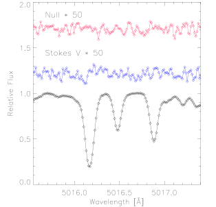
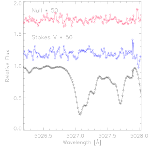
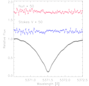
Figure 1: Example of selections on the spectra of $\epsilon$ Eri observed with HARPSpol on 5 January 2010. From the top to the bottom we reported examples of selected unblended lines, unselected blend lines and unselected strong lines.

In order to find and remove blends, we evaluated the FWHM (in ${\rm km}$ ${\rm s^{-1}}$) and the position of the centroid of each line through a gaussian fit and we discarded all the transitions whose radial velocity or the FWHM was distant more than 3$\sigma$ from the averaged value. This is possible since data were acquired with an échelle spectrograph in which $\frac{\Delta\lambda}{\lambda}\approx constant$. Fig. 1 shows examples of selected and unselected spectral lines. In average a thousand of spectral lines are selected for the measure.

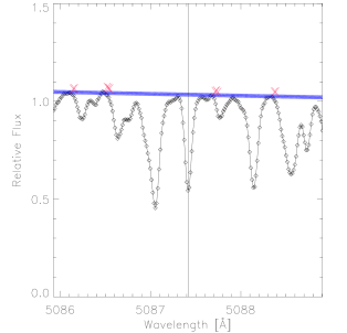
Figure 2: Example of normalisation of Stokes $I$; the linear pseudo continuum is reported in blue and the points used for the fit are in red.

Another possible source of error is the normalisation to the continuum (Bagnulo et al., 2012). In order to limit the impact, we computed the pseudo continuum level of each line through the linear fit of the highest ten points in a region of 3 Å centered on the wavelength of the transition, half on the right and half on the left (Fig. 2).

For each line (with index $j$) we computed the quantity

$${\rm x_{ij}={\rm-4.67\,10^{-13}\,\lambda_{0j}^{2}\,g_{eff_{j}}\frac{1}{I_{ij}(\lambda)}\frac{dI_{ij}(\lambda)}{d\lambda_{ij}}}}$$ (7)

where $i$ extends over the pixels. It is possible to note that Eq. 7 allows the use of the effective Landé factor $g_{{\rm eff}}$ of each particular line instead of the average value. The spectral derivative ${\rm\frac{dI_{ij}(\lambda)}{d\lambda_{ij}}}$ was computed using a 3-point Lagrange interpolation. Spikes in the spectra, due for example to cosmic rays, can affect the measurement of the magnetic field. To avoid this we performed a clipping of the null profile, rejecting all $V/I$ points whose $N/I$ is more than $5\sigma$ from the average (Bagnulo et al., 2006).

We determined the magnetic field through minimisation of $\chi^{2}$ as given by

$${\rm\chi^{2}=\sum_{ij}\frac{\left(y_{ij}-B_{eff}\,\,x_{ij}-b\right)^{2}}{\sigma_{ij}^{2}}}$$ (8)

where $b$ is a constant term related to the residual instrumental polarisation (Bagnulo et al., 2002). We used $y_{ij}=\frac{V_{ij}}{I_{ij}}$ for the measurement of the magnetic field and $y_{ij}=\frac{N_{ij}}{I_{ij}}$ for the estimation of systematic errors. This is possible because the null profile is, in principle, related to systematic errors due to observations or to the data reduction procedure. Finally, the total error was given by the quadratic sum of the systematic error and the standard error of the fit. In the case of a good measurement, we expected that the slope of $\frac{N_{ij}}{I_{ij}}$ is zero within the error range (Leone, 2007).

Fig. 3 shows an example of the magnetic field measurements obtained with the application of the multi-line slope method to high resolution spectra of the cool star $\epsilon$ Eri observed by HARPSpol using a total of 3900 lines.

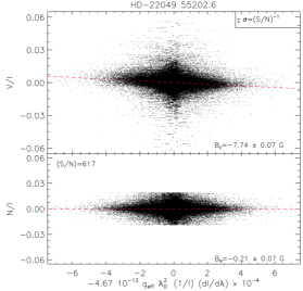
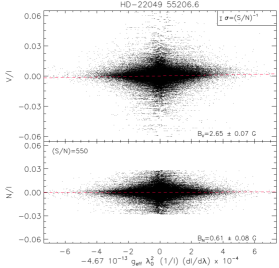
Figure 3: Magnetic field measurements of $\epsilon$ Eri from HARPSpol data. In the top panels we plot the Stokes $V$ profiles and in the bottom panels the null profiles, both as a function of the spectral derivative of Stokes $I$. The presence of the magnetic field is reflected in the slope of the distribution. The flat distribution of the null profile confirms the good quality of the measure. Figure refers, from top to the bottom, to the observation made on the nights of 5, 7 and 9 January 2010. The sizes of the typical error bar are showed in the figures; S/N is calculated from the standard deviation of the Null profile’s points.

Numerical tests

Table 1: Results of effective magnetic field measurement from the multi-line slope method ($B_{{\rm ms}}$) and from the slope method and from the slope method applied on all the simulated data points in the spectral region ($B_{\rm{slope}}$) vs rotational velocity. The input effective magnetic field is $B_{\rm inp}=-6.45$ ${\rm G}$.

				CAOS					NARVAL					HARPSpol
				R=$55000$					R=$65000$					R=$115000$
				2.5 px per FWHM					2.5 px per FWHM					4.1 px per FWHM
${\rm v}$ ${\rm sin(i)}$				Bms	$\Delta$Binp-ms	Lines	Bslope	$\Delta$Binp-slope	Bms	$\Delta$Binp-ms	Lines	Bslope	$\Delta$Binp-slope	Bms	$\Delta$Binp-ms	Lines	Bslope	$\Delta$Binp-slope
$\rm[km$ ${\rm s^{-1}]}$				${\rm[G]}$	(%)		${\rm[G]}$	(%)	${\rm[G]}$	(%)		${\rm[G]}$	(%)	${\rm[G]}$	(%)		${\rm[G]}$	(%)
0				-6.59	2	697	-8.60	33	-6.69	4	697	-8.46	31	-6.33	-2	697	-7.72	20
3				-7.28	13	688	-9.18	42	-7.21	12	688	-9.12	41	-7.08	10	688	-8.83	37
6				-8.13	26	615	-10.04	56	-8.24	28	615	-10.15	57	-8.20	27	615	-10.17	58
9				-8.49	32	537	-10.57	64	-8.66	34	537	-10.67	65	-8.57	33	537	-10.53	63
12				-8.53	32	411	-10.72	66	-8.51	32	411	-10.70	66	-8.44	31	411	-10.48	63
15				-8.74	35	301	-10.74	66	-8.69	35	301	-10.67	65	-8.50	32	301	-10.43	62
18				-8.85	37	236	-10.80	67	-8.64	34	236	-10.57	64	-8.54	32	236	-10.43	62
21				-8.99	39	187	-10.74	67	-9.08	41	187	-10.66	65	-8.80	36	187	-10.39	61
24				-9.43	46	146	-10.77	67	-9.31	44	146	-10.57	64	-9.17	42	146	-10.31	60
27				-9.29	44	104	-10.60	64	-9.40	46	104	-10.67	65	-9.23	43	104	-10.29	60
30				-9.92	54	61	-10.58	64	-10.37	61	61	-10.65	65	-10.02	55	61	-10.29	60
33				-10.79	67	48	-10.76	67	-10.31	60	48	-10.80	67	-10.25	59	48	-10.34	60

Table 2: Results of effective magnetic field measurement from the multi-line slope method ($B_{{\rm ms}}$) and from the slope method applied on all the simulated data points in the spectral region from 500 nm to 600 nm ($B_{\rm{slope}}$) vs effective magnetic field strength. The rotational velocity is ${\rm v}$ ${\rm sin(i)}$=3 ${\rm km}$ ${\rm s^{-1}}$.

				CAOS					NARVAL					HARPSpol
				R=$55000$					R=$65000$					R=$115000$
				2.5 px per FWHM					2.5 px per FWHM					4.1 px per FWHM
Binp				Bms	$\Delta$Binp-ms	Lines	Bslope	$\Delta$Binp-slope	Bms	$\Delta$Binp-ms	Lines	Bslope	$\Delta$Binp-slope	Bms	$\Delta$Binp-ms	Lines	Bslope	$\Delta$Binp-slope
${\rm[G]}$				${\rm[G]}$	(%)		${\rm[G]}$	(%)	${\rm[G]}$	(%)		${\rm[G]}$	(%)	${\rm[G]}$	(%)		${\rm[G]}$	(%)
0.63				0.66	5	1344	0.91	43	0.72	13	1344	0.93	46	0.70	10	1344	0.89	40
6.35				7.37	16	1342	9.23	45	7.17	13	1342	9.09	43	7.07	11	1342	8.87	40
65				75	18	1348	91	44	75	18	1348	91	43	73	15	1348	88	39
635				684	8	1341	819	29	681	7	1341	815	28	649	2	1341	788	24
3175				2323	-27	675	2740	-14	2155	-32	675	2495	-21	1516	-52	675	1697	-47

Table 3: Results of effective magnetic field measurement from the multi-line slope method ($B_{\rm ms}$) vs S/N ratio. The input effective magnetic field is $B_{inp}=6.35$ G and ${\rm v}$ ${\rm sin(i)}$=3 ${\rm km}$ ${\rm s^{-1}}$. $\sigma$B_ms is the standard deviation of the measures in the simulation (details in the text). The spectral region is between 500 nm to 600 nm.

				CAOS				NARVAL				HARPSpol
				R=$55000$				R=$65000$				R=$115000$
				2.5 px per FWHM				2.5 px per FWHM				4.1 px per FWHM
S/N				Bms	$\sigma$Bms	$\Delta$Binp-ms	Lines	Bms	$\sigma$Bms	$\Delta$Binp-ms	Lines	Bms	$\sigma$Bms	$\Delta$Binp-ms	Lines
				${\rm[G]}$	${\rm[G]}$	(%)		${\rm[G]}$	${\rm[G]}$	(%)		${\rm[G]}$	${\rm[G]}$	(%)
100				4.18	5.50	-34	1274	6.13	4.88	-3	1348	5.98	1.66	-6	1537
250				8.13	1.88	28	1310	7.34	2.21	16	1375	6.90	0.63	9	1512
500				7.18	1.62	13	1322	7.14	0.66	12	1382	6.76	0.34	6	1517
1000				7.41	0.50	17	1333	7.13	0.34	12	1389	6.92	0.18	9	1519

Table 4: Results of the effective magnetic field measurement from the multi-line slope method ($B_{{\rm ms}}$) and from the slope method applied on all the simulated data points in a region from 500 nm to 550 nm ($B_{\rm{slope}}$) in the case of decentered dipole model for the magnetic field geometry.

				CAOS					NARVAL					HARPSpol
				R=$55000$					R=$65000$					R=$115000$
				2.5 px per FWHM					2.5 px per FWHM					4.1 px per FWHM
Binp				Bms	$\Delta$Binp-ms	Lines	Bslope	$\Delta$Binp-slope	Bms	$\Delta$Binp-ms	Lines	Bslope	$\Delta$Binp-slope	Bms	$\Delta$Binp-ms	Lines	Bslope	$\Delta$Binp-slope
${\rm[G]}$				${\rm[G]}$	(%)		${\rm[G]}$	(%)	${\rm[G]}$	(%)		${\rm[G]}$	(%)	${\rm[G]}$	(%)		${\rm[G]}$	(%)
-1.45				-1.34	-7	350	-1.77	22	-1.34	-8	362	-1.78	23	-1.26	-13	384	-1.70	17

To test the capabilities of the multi-line slope method we computed synthetic spectra using COSSAM (Codice per la Sintesi Spettrale nelle Atmosfere Magnetiche) (Stift et al., 2012). It is a fully parallelised code that solves the polarised radiative transfer equation for a stellar atmosphere permeated by a magnetic field under the assumption of local thermal equilibrium (LTE). The code calculates the emergent Stokes $IQUV$ spectrum integrated over the visible stellar disk. Details of design decisions and implementation can be found in Stift & Dubois (1998) and Stift (1998).

All synthetic profiles were convolved with the respective FWHM of CAOS, NARVAL and HARPSpol and resampled to conform with the wavelength binnings. Simulations were performed considering a dipolar magnetic field geometry centered on the star, with ${\rm i=135}$°, ${\beta=50}$°, considering a zero phase.

First, we tested the effects of the rotational velocity on the measurements; results are shown in Table 1. One can see that for very low values of rotational velocity (lower than 5 ${\rm km}$ ${\rm s^{-1}}$), the results of the multi-line slope method differ with respect to the input by the order of 20%. This difference increases with rotational velocity, and for ${\rm v}\,{\rm sin(i)}$ > 30 ${\rm km}$ ${\rm s^{-1}}$ it exceeds 50%. For this we blame large rotational velocity values which affect the shape of the line profile and its derivative in a non-negligible way.

A second simulation tests the effects of the field strength in the measure, in the case of low rotational velocity (${\rm v}$ ${\rm sin(i)}$ = 3 ${\rm km}$ ${\rm s^{-1}}$). We can see from Table 2 that the multi-line slope method gives results which differ by some 20% from the input value for field strength less than 1000 G. For values larger than 1000 G, the method underestimates the field with the discrepancy increasing with the spectral resolution. These findings may be explained by the fact that with higher resolution and higher field values Zeeman splitting is dominant and so the first derivative of Stokes $I$ is no longer simply related to Stokes $V$ through Eq. 6.

We can conclude that the assumption of small velocity broadening made in Eq. 6 is valid. Therefore, in the case of very low stellar rotational velocity – ${\rm v}$ ${\rm sin(i)}$ < 5 ${\rm km}$ ${\rm s^{-1}}$ – and low effective field strength – ${\rm B_{eff}<1kG}$ – the multi-line slope method is a valid technique for measuring the effective magnetic field.

The simulations of Table 1 and Table 2 also show the advantage of the multi-line approach. Indeed we can note how the technique allows to retrieve results closer to the input, better than 20% with respect to the slope method applied on all the simulated data points in the spectral region; this behaviour is systematic, except for the case of large field strengths.

The first two simulations were computed without consider the effects of the degradation due to the photon noise. A third simulation tests the capabilities of the multi-line slope method to retrieve the effective magnetic field with spectra of finite S/N ratio.

For each point in the synthetic spectra, we generated a random number, from a normal distribution with a mean zero and a standard deviation of one, and we divided it by the wanted value of S/N and by the square root of the synthetic Stokes $I$. This noise $\eta$ was added on the combination of Stokes profiles:

$$\begin{array}[]{c}{\rm s_{1}=(I+V)+\eta}\\ {\rm s_{2}=(I-V)+\eta}\end{array}$$ (9)

that can be used to compute the noise synthetic profiles $\widetilde{\rm I}$ and $\widetilde{\rm V}$ through:

$$\begin{array}[]{c}{\rm\widetilde{I}=\frac{s_{1}+s_{2}}{2}}\\ {\rm\widetilde{V}=\frac{s_{1}-s_{2}}{2}}\end{array}$$ (10)

Each measure was repeated 100 times with different random numbers, in order to compute the average B_ms and the standard deviation $\sigma$B_ms.

Results of Table 3 show that, for low field values, the errors and the differences between input and results decrease at higher resolution. The simulations reveal that a minimum S/N of 250 is needed in Stokes $V$ in order to measure the effective magnetic field with an error lower than 3$\sigma$, in the case of CAOS resolution.

All the previous simulation were computed considering a dipolar magnetic field geometry, centered on the star. In order to test the impact of the different geometry, we performed a measure considering a more general model, using a decentered dipole (Stift, 1974). Results on Table 4 shows that the method can be applied also in this case and, for this reason, we can conclude that choice of dipolar configuration do not impact the measure.

5 Comparison with the Least Squares Deconvolution (LSD) technique

Magnetic field measurements from high resolution spectropolarimetric data are often made using Least Squares Deconvolution. This method is based on the assumption that all the spectral lines have the same profile and that they can be added linearly. The LSD method can extract an average Stokes profile that can be used for the measurement of the effective magnetic field through the first order moment of LSD Stokes $V$ (Kochukhov et al., 2010):

$${\rm B_{eff}=-7.145\,\times\,10^{6}\frac{\int v\,Z^{v}\,dv}{\lambda_{0}\bar{g}\int Z^{I}\,dv}}$$ (11)

where $Z^{v}$ is the Stokes $V$ LSD profile, $Z^{I}$ the Stokes $I$ LSD profile, $\lambda_{0}$ and $\bar{g}$ are (arbitrary) quantities adopted for the normalisation of weights of the Stokes $V$ LSD profile.

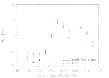
Figure 4: Comparison between the multi-line slope method (black) and LSD (red) for the $\epsilon$ Eri HARPSpol observations of January 2010 (Piskunov et al., 2011; Olander, 2013).

In order to compare the results of the multi-line slope method with the LSD results, we measure the effective magnetic field of $\epsilon$ Eri from the observations of HARPSpol made in 2010, published by Piskunov et al. (2011). The quantitative values of the LSD measures are taken from Olander (2013). We can see in Fig. 4 that in general the results are in agreement; however the multi-line slope method gives results systematically lower than the LSD measures. The reasons for this have yet to be determined.

We conclude that the multi-line slope method can be used as an alternative technique to LSD for the measurement of the effective magnetic fields of cool stars. It has the advantage of being easier and faster to compute; on the other hand, LSD can retrieve the shape of the profile, allowing the detection of magnetic field configurations with zero average value. At least in principle, the slope method can also point out a zero average field when the $V/I$ scatter is larger than $N/I$ scatter.

6 The magnetic field of $\epsilon$ Eridani

Figure 5: Magnetic curves of $\epsilon$ Eri folded with the period of rotation of the star $P_{rot}=11.35$ d (Fröhlich, 2007). Cross, diamonds and plus refers to observations obtained respectively with NARVAL, HARPSpol and CAOS. Zero phase is equal to MJD 54101 (Jeffers et al., 2014). Magnetic curves are obtained by a fitting through Eq. 12 (see text).

Epsilon Eridani (HD 22049, HIP 16537) is one of the brightest and best studied solar analogues. It is a K2V star with an effective temperature of $5146$ K, a mass of 0.856 M_☉ and ${\rm v}$  ${\rm sin(i)}=2.4$ ${\rm km}$ ${\rm s^{-1}}$ (Valenti & Fischer, 2005). Infrared observations show that the star is surrounded by a debris disk (Greaves et al., 2005) with density inhomogeneities that can be explained by the existence of exoplanets (Backman et al., 2009).

Actually, the existence of planets in the system orbiting $\epsilon$ Eri is an open question. Hatzes et al. (2000) ascribed the long-period radial velocity (RV) variation to the presence of a planetary companion. This presence was confirmed by Benedict et al. (2006) who estimated a period $P_{\rm orbital}=6.85\pm 0.03$ yr and a companion mass of $M=1.55\pm 0.24$ M_J. Anglada-Escudé & Butler (2012) however concluded that the RV variability of $\epsilon$ Eri is probably due to stellar activity cycles (not strictly periodic) rather than to the presence of a planet. The presence of a planet was not confirmed from the velocity measurements analysed by Zechmeister et al. (2013) nor from imaging either (Janson et al., 2015; Mizuki et al., 2016).

The stellar activity of $\epsilon$ Eri over 45 years was studied by Metcalfe et al. (2013) who found a short cycle of 2.95 yr modulated by a long cycle of 12.7 yr. The magnetic field could play an important role in this star. In order to study the long term variation of it, Jeffers et al. (2014) performed spectropolarimetric observations; they collected Stokes $I$ and $V$ profiles at six epochs in a range of seven years, using the spectropolarimeters NARVAL and HARPSpol. They found that the large-scale magnetic field is highly variable, with no common pattern over the years, and they concluded that more observations were needed to investigate the magnetic activity of $\epsilon$ Eri.

Table 5: Effective magnetic field measures of $\epsilon$Eri.

MJD		$B_{{\rm eff}}$ [G]		Instrument		MJD		$B_{{\rm eff}}$ [G]		Instrument
54122.256		-12.97 $\pm$	0.21		NARVAL	55605.505		2.15 $\pm$	0.25		HARPS
54127.316		7.49 $\pm$	0.60		NARVAL	55606.504		0.72 $\pm$	0.16		HARPS
54128.313		7.53 $\pm$	0.31		NARVAL	55836.623		6.80 $\pm$	0.05		NARVAL
54130.354		0.69 $\pm$	0.26		NARVAL	55838.638		7.94 $\pm$	0.10		NARVAL
54133.326		-14.41 $\pm$	0.11		NARVAL	55843.622		4.53 $\pm$	0.14		NARVAL
54135.316		-9.87 $\pm$	0.18		NARVAL	55845.503		4.39 $\pm$	0.09		NARVAL
54140.328		6.43 $\pm$	0.12		NARVAL	55846.521		4.85 $\pm$	0.44		NARVAL
54485.380		-3.83 $\pm$	0.37		NARVAL	55850.517		9.00 $\pm$	0.12		NARVAL
54487.305		-1.00 $\pm$	0.06		NARVAL	55866.516		1.32 $\pm$	0.14		NARVAL
54488.321		-1.69 $\pm$	0.06		NARVAL	55874.464		11.18 $\pm$	0.12		NARVAL
54489.325		-3.68 $\pm$	0.21		NARVAL	55876.594		7.16 $\pm$	0.15		NARVAL
54490.345		-7.72 $\pm$	0.21		NARVAL	55877.552		4.95 $\pm$	0.13		NARVAL
54491.328		-9.77 $\pm$	0.33		NARVAL	55882.540		4.54 $\pm$	0.19		NARVAL
54492.327		-10.31 $\pm$	0.29		NARVAL	55887.432		9.88 $\pm$	0.08		NARVAL
54493.339		-9.36 $\pm$	0.08		NARVAL	56202.533		1.14 $\pm$	0.07		NARVAL
54494.383		-7.37 $\pm$	0.06		NARVAL	56203.533		1.07 $\pm$	0.23		NARVAL
54495.352		-7.01 $\pm$	0.08		NARVAL	56205.556		-3.79 $\pm$	0.17		NARVAL
54499.348		2.53 $\pm$	0.17		NARVAL	56206.543		-3.74 $\pm$	0.10		NARVAL
54501.331		-5.01 $\pm$	0.06		NARVAL	56214.494		-4.65 $\pm$	0.39		NARVAL
54502.330		-9.18 $\pm$	0.17		NARVAL	56224.617		-3.89 $\pm$	0.13		NARVAL
54503.330		-9.60 $\pm$	0.14		NARVAL	56229.541		-5.57 $\pm$	0.26		NARVAL
54506.339		-7.12 $\pm$	0.08		NARVAL	56230.540		-0.56 $\pm$	0.19		NARVAL
54507.284		-8.19 $\pm$	0.27		NARVAL	56232.517		5.25 $\pm$	0.07		NARVAL
54508.342		-6.94 $\pm$	0.07		NARVAL	56238.554		-11.85 $\pm$	0.14		NARVAL
54509.347		-3.64 $\pm$	0.20		NARVAL	56244.508		4.31 $\pm$	0.16		NARVAL
54510.343		0.45 $\pm$	0.29		NARVAL	56246.476		-0.15 $\pm$	0.38		NARVAL
54511.350		-0.11 $\pm$	0.07		NARVAL	56254.483		0.02 $\pm$	0.49		NARVAL
54512.341		-2.49 $\pm$	0.16		NARVAL	56555.500		-3.44 $\pm$	0.05		NARVAL
55199.609		-4.04 $\pm$	0.04		HARPS	56556.500		0.56 $\pm$	0.06		NARVAL
55200.593		-7.02 $\pm$	0.27		HARPS	56557.500		3.50 $\pm$	0.23		NARVAL
55201.650		-8.48 $\pm$	0.08		HARPS	56575.500		-17.29 $\pm$	0.10		NARVAL
55202.593		-7.74 $\pm$	0.13		HARPS	56576.500		-11.61 $\pm$	0.14		NARVAL
55203.550		-5.54 $\pm$	0.37		HARPS	56577.500		-4.70 $\pm$	0.28		NARVAL
55204.569		-0.20 $\pm$	0.16		HARPS	56578.500		-2.34 $\pm$	0.13		NARVAL
55205.593		4.19 $\pm$	0.14		HARPS	56921.608		6.02 $\pm$	1.64		CAOS
55206.570		2.65 $\pm$	0.35		HARPS	56922.557		5.67 $\pm$	0.42		CAOS
55207.617		-0.66 $\pm$	0.06		HARPS	56922.578		4.52 $\pm$	0.20		CAOS
55209.558		2.52 $\pm$	0.13		HARPS	56941.499		2.12 $\pm$	0.49		CAOS
55210.587		0.62 $\pm$	0.11		HARPS	56946.504		-0.36 $\pm$	2.12		CAOS
55211.575		-3.27 $\pm$	0.14		HARPS	56947.504		-3.12 $\pm$	2.54		CAOS
55224.311		-5.36 $\pm$	0.08		NARVAL	56949.551		-1.12 $\pm$	0.16		CAOS
55231.306		-2.42 $\pm$	0.72		NARVAL	57044.323		4.65 $\pm$	0.15		CAOS
55241.276		5.21 $\pm$	0.31		NARVAL	57630.549		-10.58 $\pm$	1.39		CAOS
55242.271		1.78 $\pm$	0.12		NARVAL	57630.580		-6.10 $\pm$	2.34		CAOS
55600.534		-1.66 $\pm$	0.05		HARPS	57634.617		-6.12 $\pm$	1.31		CAOS
55601.509		-0.78 $\pm$	0.09		HARPS	57723.443		-6.41 $\pm$	1.64		CAOS
55602.599		-1.44 $\pm$	0.04		HARPS	57724.413		-9.74 $\pm$	2.13		CAOS

The multi-line slope method measures of all available high resolution spectropolarimetric data are reported in Table 5. Fig. 5 shows the highly variable behaviour of the effective magnetic field of the star, folded with the rotational period; we noted that some curves are characterised by a change of polarity of the field (Narval 2007, HARPSpol 2010 and Narval 2013), in others the magnetic field has the same sign as in the case of NARVAL 2011. Sinusoidal fits, showed in Fig. 5, are obtained using:

$${\rm f(t)=A_{0}+A_{1}\,sin\left(2\pi\,\frac{t-t_{0}}{P}+A_{2}\right)+A_{3}\,sin\left(4\pi\,\frac{t-t_{0}}{P}+A_{4}\right)}$$ (12)

where ${\rm t}$ is the time in days, ${\rm t_{0}}$ is a reference time equal to MJD 54101 (Jeffers et al., 2014), ${\rm P}$ is the variability period assumed as the rotational one, ${\rm A_{1}}$ and ${\rm A_{3}}$ are amplitudes (expressed in Gauss), ${\rm A_{2}}$ and ${\rm A_{4}}$ are phase shifts and ${\rm A_{0}}$ represents the level of the variation of the curves (in Gauss); fit of the data of CAOS and HARPS 2011 are obtained using a single wave (${\rm A_{3}}={\rm A_{4}}=0$) because the few number of measured points in their magnetic curves and the magnetic curve of Jan 2010 is obtained using both HARPSpol and NARVAL data.

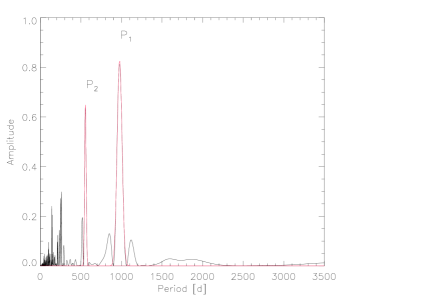
Figure 6: Top: Cleaned Fourier transform of the effective magnetic field of $\epsilon$ Eri (black) (Deeming, 1975; Roberts et al., 1987) and gaussian fit of the main periods (red). Bottom: Effective magnetic field measures (Table 5) folded with the two periods. Cross, diamonds and plus refers to observations obtained respectively with NARVAL, HARPSpol and CAOS.

Figure 7: S-index measures (Metcalfe et al., 2013) folded with the period $P_{1}$.

In order to find periodicities in the effective magnetic field we computed the Fourier transform following Deeming (1975). We deconvolved in the frequency domain using the CLEAN algorithm (Roberts et al., 1987) in order to limit the effects of artefacts caused by the incompleteness of the sampling. The results are reported in Fig. 6. Fitting a Gaussian, we estimated the position of the main peaks at $P_{1}=976\pm 70$ d and $P_{2}=555\pm 22$ d; errors are assumed to be as large as the FWHM of the Gaussian. We noted that $P_{1}$ is close to the 2.95 yr period found by Metcalfe et al. (2013) (Fig. 7). Indeed, the period corresponds to that one found by Lehmann et al. (2015) analysis the magnetic field from the Zeeman broadening.

Table 6: Table of the values of A₀.

MJDaverage		A0
		[G]
54131.030		-3.15 $\pm$	0.21
54498.337		-6.08 $\pm$	0.03
55205.339		-2.19 $\pm$	0.04
55603.330		-0.31 $\pm$	0.04
55860.543		7.12 $\pm$	0.03
56225.684		-0.58 $\pm$	0.04
56568.214		-8.27 $\pm$	0.67
56949.516		2.34 $\pm$	0.67
57668.720		-8.17 $\pm$	0.67

Another analysis can be performed on the variation of the level of the curves ${\rm A_{0}}$. This is done in order to separate the short-time sinusoidal variations – due to stellar rotation – from long-term changes in the constant term ${\rm A_{0}}$, obtained by Eq. 12. The values of ${\rm A_{0}}$ are reported in Table 6 with the average time of the magnetic curves. The Fourier transform (Fig. 8) exhibits periods near to those of the effective magnetic field at $P_{1}=1099\pm 71$ d and $P_{2}=517\pm 17$ d. In order to find the best period we computed $\chi^{2}$ for a sinusoidal fit to the ${\rm A_{0}}$ values, folded with the two periods. The results, reported in the bottom panel of Fig. 8, reveal that $P_{1}$ is the best period.

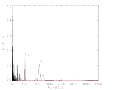
Figure 8: Top: Cleaned Fourier transform of $A_{0}$ (black) (Deeming, 1975; Roberts et al., 1987) and gaussian fit of the main periods (red). Bottom: $A_{0}$ folded with the two periods.

7 Conclusion

We have introduced an extension to a method developed by Bagnulo et al. (2002) for measuring the effective magnetic field of stars from low resolution spectropolarimetry by means of a regression of Stokes $V$ against the spectral derivative of Stokes $I$. Our multi-line slope method, based on high resolution spectropolarimetry, instead uses similar information from the Stokes profiles of a large number of unblended lines. We carried out tests of the new method, using the polarised radiative transfer code Cossam, concluding that results are satisfactory for stars with low rotational velocities (${\rm v}$ ${\rm sin(i)}$ < 5 ${\rm km}$ ${\rm s^{-1}}$) and field strengths (${\rm B_{eff}<1kG}$).

The comparison with the popular Least Square Deconvolution shows that the multi-line slope method can be an easy-to-use and fast alternative for measuring the effective magnetic field of late-type stars. LSD on the other hand offers the advantage of retrieving the shape of the Stokes profile; this makes it possible to infer the presence of a magnetic field with zero average value.

Finally, we applied the technique to all the available spectropolarimetric data of the star $\epsilon$ Eri. We separated the short-time variation of the effective magnetic field, due to stellar rotation, from the long-term variation through the coefficient $A_{0}$ (defined in Eq. 12); we used a Fourier transform to discover that the best-fit period of the variation of $A_{0}$ ($P_{1}=1099\pm 71$ d) is close to the short cycle period in the S-index found by Metcalfe et al. (2013) and to the period of the magnetic field found by the analysis of the Zeeman broadening (Lehmann et al., 2015). Direct measurements of the effective magnetic field thus open up the possibility to determine the periods of the cycles of active cool stars.

References

- Anglada-Escudé & Butler (2012) Anglada-Escudé G., Butler R. P., 2012, ApJS, 200, 15
- Aurière (2003) Aurière M., 2003, in Arnaud J., Meunier N., eds, EAS Publications Series Vol. 9, EAS Publications Series. p. 105
- Backman et al. (2009) Backman D., et al., 2009, ApJ, 690, 1522
- Bagnulo et al. (2002) Bagnulo S., Szeifert T., Wade G. A., Landstreet J. D., Mathys G., 2002, A&A, 389, 191
- Bagnulo et al. (2006) Bagnulo S., Landstreet J. D., Mason E., Andretta V., Silaj J., Wade G. A., 2006, A&A, 450, 777
- Bagnulo et al. (2012) Bagnulo S., Landstreet J. D., Fossati L., Kochukhov O., 2012, A&A, 538, A129
- Benedict et al. (2006) Benedict G. F., et al., 2006, AJ, 132, 2206
- Bouvier et al. (2007) Bouvier J., et al., 2007, A&A, 463, 1017
- Carolo et al. (2014) Carolo E., et al., 2014, A&A, 567, A48
- Deeming (1975) Deeming T. J., 1975, Ap&SS, 36, 137
- Desidera et al. (2004) Desidera S., et al., 2004, A&A, 420, L27
- Donati et al. (1997) Donati J.-F., Semel M., Carter B. D., Rees D. E., Collier Cameron A., 1997, MNRAS, 291, 658
- Dumusque et al. (2012) Dumusque X., et al., 2012, Nature, 491, 207
- Fröhlich (2007) Fröhlich H.-E., 2007, Astronomische Nachrichten, 328, 1037
- Greaves et al. (2005) Greaves J. S., et al., 2005, ApJ, 619, L187
- Hatzes et al. (2000) Hatzes A. P., et al., 2000, ApJ, 544, L145
- Hubrig et al. (2016) Hubrig S., Scholz K., Hamann W.-R., Schöller M., Ignace R., Ilyin I., Gayley K. G., Oskinova L. M., 2016, MNRAS, 458, 3381
- Janson et al. (2015) Janson M., Quanz S. P., Carson J. C., Thalmann C., Lafrenière D., Amara A., 2015, A&A, 574, A120
- Jeffers et al. (2014) Jeffers S. V., Petit P., Marsden S. C., Morin J., Donati J.-F., Folsom C. P., 2014, A&A, 569, A79
- Judge & Thompson (2012) Judge P. G., Thompson M. J., 2012, in Mandrini C. H., Webb D. F., eds, IAU Symposium Vol. 286, Comparative Magnetic Minima: Characterizing Quiet Times in the Sun and Stars. pp 15–26 (arXiv:1201.4625), doi:10.1017/S1743921312004589
- Kane et al. (2016) Kane S. R., et al., 2016, ApJ, 820, L5
- Kochukhov et al. (2010) Kochukhov O., Makaganiuk V., Piskunov N., 2010, A&A, 524, A5
- Kolenberg & Bagnulo (2009) Kolenberg K., Bagnulo S., 2009, A&A, 498, 543
- Kurucz (1993) Kurucz R. L., 1993, SYNTHE spectrum synthesis programs and line data
- Landstreet (1982) Landstreet J. D., 1982, ApJ, 258, 639
- Lehmann et al. (2015) Lehmann L. T., Künstler A., Carroll T. A., Strassmeier K. G., 2015, Astronomische Nachrichten, 336, 258
- Leone (2007) Leone F., 2007, MNRAS, 382, 1690
- Leone et al. (2011) Leone F., Martínez González M. J., Corradi R. L. M., Privitera G., Manso Sainz R., 2011, ApJ, 731, L33
- Leone et al. (2016) Leone F., et al., 2016, AJ, 151, 116
- Metcalfe et al. (2013) Metcalfe T. S., et al., 2013, ApJ, 763, L26
- Mizuki et al. (2016) Mizuki T., et al., 2016, A&A, 595, A79
- Morgenthaler et al. (2010) Morgenthaler A., et al., 2010, in Boissier S., Heydari-Malayeri M., Samadi R., Valls-Gabaud D., eds, SF2A-2010: Proceedings of the Annual meeting of the French Society of Astronomy and Astrophysics. p. 269 (arXiv:1012.0198)
- Olander (2013) Olander T., 2013, The magnetic field of ε Eri
- Petit et al. (2014) Petit P., Louge T., Théado S., Paletou F., Manset N., Morin J., Marsden S. C., Jeffers S. V., 2014, PASP, 126, 469
- Pevtsov et al. (2003) Pevtsov A. A., Fisher G. H., Acton L. W., Longcope D. W., Johns-Krull C. M., Kankelborg C. C., Metcalf T. R., 2003, ApJ, 598, 1387
- Piskunov et al. (1995) Piskunov N. E., Kupka F., Ryabchikova T. A., Weiss W. W., Jeffery C. S., 1995, A&AS, 112, 525
- Piskunov et al. (2011) Piskunov N., et al., 2011, The Messenger, 143, 7
- Preusse et al. (2006) Preusse S., Kopp A., Büchner J., Motschmann U., 2006, A&A, 460, 317
- Queloz et al. (2001) Queloz D., et al., 2001, A&A, 379, 279
- Reiners (2012) Reiners A., 2012, Living Reviews in Solar Physics, 9
- Roberts et al. (1987) Roberts D. H., Lehar J., Dreher J. W., 1987, AJ, 93, 968
- Sbordone et al. (2004) Sbordone L., Bonifacio P., Castelli F., Kurucz R. L., 2004, Memorie della Societa Astronomica Italiana Supplementi, 5, 93
- Schrijver et al. (1989) Schrijver C. J., Cote J., Zwaan C., Saar S. H., 1989, ApJ, 337, 964
- Semel & Li (1996) Semel M., Li J., 1996, Sol. Phys., 164, 417
- Semel et al. (2009) Semel M., Ramírez Vélez J. C., Martínez González M. J., Asensio Ramos A., Stift M. J., López Ariste A., Leone F., 2009, A&A, 504, 1003
- Sennhauser & Berdyugina (2010) Sennhauser C., Berdyugina S. V., 2010, A&A, 522, A57
- Snik et al. (2011) Snik F., et al., 2011, in Kuhn J. R., Harrington D. M., Lin H., Berdyugina S. V., Trujillo-Bueno J., Keil S. L., Rimmele T., eds, Astronomical Society of the Pacific Conference Series Vol. 437, Solar Polarization 6. p. 237 (arXiv:1010.0397)
- Stift (1974) Stift M. J., 1974, MNRAS, 169, 471
- Stift (1998) Stift M. J., 1998, (Astro)physical supercomputing: Ada95 as a safe, object oriented alternative. Springer Berlin Heidelberg, Berlin, Heidelberg, pp 128–139, doi:10.1007/BFb0055000, http://dx.doi.org/10.1007/BFb0055000
- Stift & Dubois (1998) Stift M. J., Dubois P. F., 1998, Computers in Physics, 12, 150
- Stift et al. (2012) Stift M. J., Leone F., Cowley C. R., 2012, MNRAS, 419, 2912
- Strugarek et al. (2015) Strugarek A., Brun A. S., Matt S. P., Réville V., 2015, ApJ, 815, 111
- Tinbergen & Rutten (1992) Tinbergen J., Rutten R., 1992
- Unno (1956) Unno W., 1956, PASJ, 8, 108
- Valenti & Fischer (2005) Valenti J. A., Fischer D. A., 2005, ApJS, 159, 141
- Zechmeister et al. (2013) Zechmeister M., et al., 2013, A&A, 552, A78