Hyperspectral Unmixing: Ground Truth Labeling, Datasets, Benchmark Performances and Survey

Abstract

Hyperspectral unmixing (HU) is a very useful and increasingly popular preprocessing step for a wide range of hyperspectral applications. However, the HU research has been constrained a lot by three factors: (a) the number of hyperspectral images (especially the ones with ground truths) are very limited; (b) the ground truths of most hyperspectral images are not shared on the web, which may cause lots of unnecessary troubles for researchers to evaluate their algorithms; (c) the codes of most state-of-the-art methods are not shared, which may also delay the testing of new methods.

Accordingly, this paper deals with the above issues from the following three perspectives: (1) as a profound contribution, we provide a general labeling method for the HU. With it, we labeled up to 15 hyperspectral images, providing 18 versions of ground truths. To the best of our knowledge, this is the first paper to summarize and share up to 15 hyperspectral images and their 18 versions of ground truths for the HU. Observing that the hyperspectral classification (HyC) has much more standard datasets (whose ground truths are generally publicly shared) than the HU, we propose an interesting method to transform the HyC datasets for the HU research. (2) To further facilitate the evaluation of HU methods under different conditions, we reviewed and implemented the algorithm to generate a complex synthetic hyperspectral image. By tuning the hyper-parameters in the code, we may verify the HU methods from four perspectives. The code would also be shared on the web. (3) To provide a standard comparison, we reviewed up to 10 state-of-the-art HU algorithms, then selected the 5 most benchmark HU algorithms, and compared them on the 15 real hyperspectral datasets. The experiment results are surely reproducible; the implemented codes would be shared on the web.

I Introduction

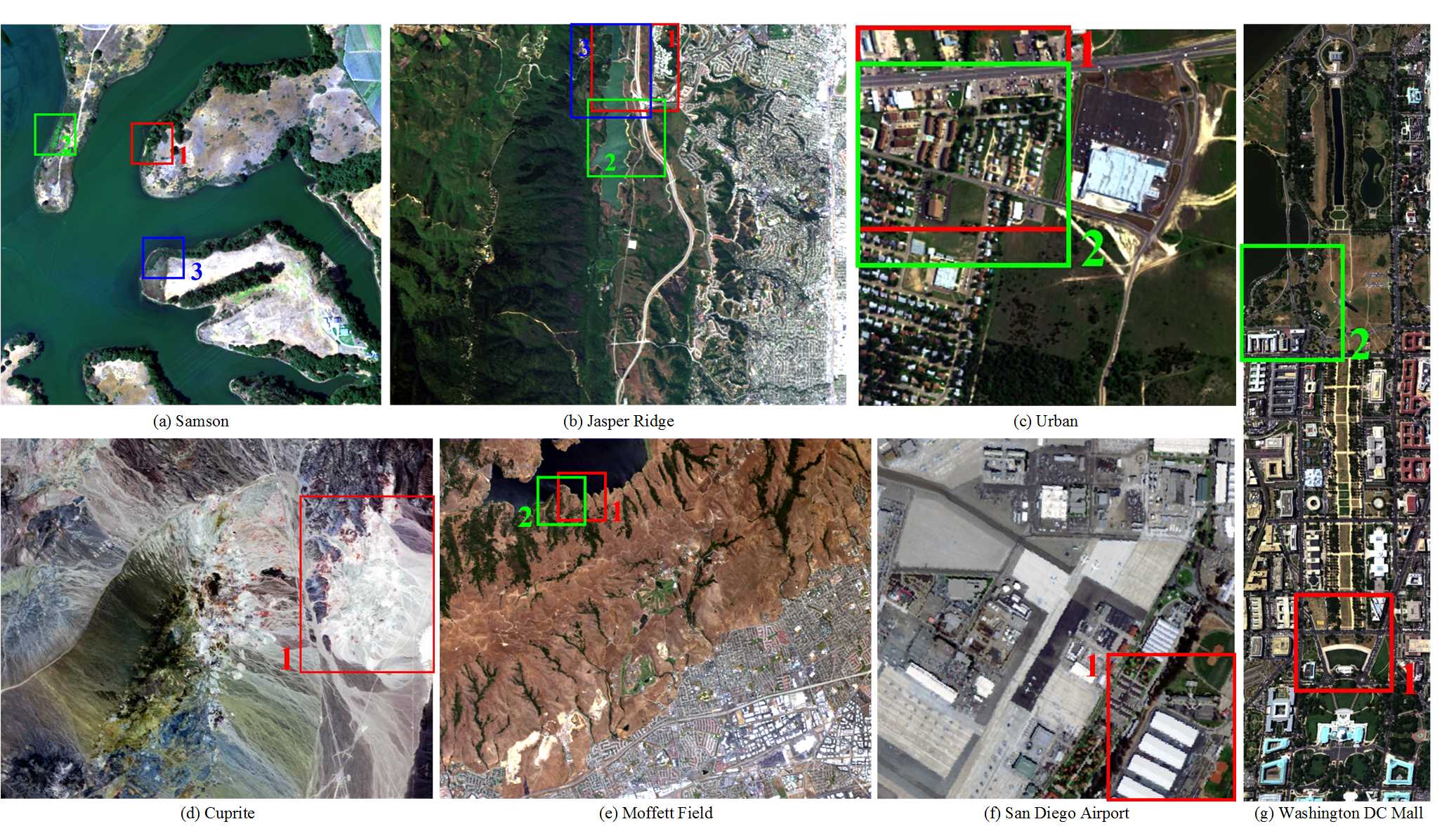
Figure 1: The illustration of 7 popular hyperspectral images where we select 15 subimages (i.e., ROIs) and provide 18 versions of ground truths for the HU study. They are [a] Samson (3 ROIs), [b] Jasper Ridge (3 ROIs), [c] Urban (the full image and 2 ROIs), [d] Cuprite (1 ROI), [e] Moffett Field (2 ROIs), [f] San Diego Airport (1 ROI), and [g] Washington DC Mall (2 ROIs). In Section V and Table I, we provide very detailed information about the 15 ROIs.

Hyperspectral remote sensing has been widely used in lots of applications since it can capture a 3D image cube at hundreds of contiguous bands across the electromagnetic spectrum, providing substantial information of the scene [1]. However, due to the microscopic material mixing, multiple scattering and low spatial resolution of hyperspectral sensors, the pixel spectra are inevitably mixed with various substances [2, 1], resulting in lots of mixed pixels. Accordingly, hyperspectral unmixing (HU) is an essential processing step for various hyperspectral image applications, such as high-resolution hyperspectral imaging [3, 4, 5, 6, 7, 8], hyperspectral enhancement [9], sub-pixel mapping [10], hyperspectral compression and reconstruction [11], detection and identification substances in the scene [9, 12], hyperspectral visualization [13, 14], etc.

TABLE I: The 15 real hyperspectral (sub-) images and their information, including the image size, the numbers of all spectral bands and the selected bands, the endmembers numbers, the illustration of scenes and their 18 versions of ground truths etc.

Real Datasets	Image sizes		Number of bands		# End-	Ground truth	The top-left pixel in	Subimages
	# row	# column	# all bands	# selected bands	member	shown in	original image	shown in
1. Samson#1	95	95	156	156	3	Fig. 2a	$\left(252,\,332\right)$	Fig. 1a
2. Samson#2	95	95			3	Fig. 2b	$\left(232,\,93\right)$
3. Samson#3	95	95			3	Fig. 2c	$\left(634,\,455\right)$
4. Jasper Ridge#1	115	115	224	198	5	Fig. 3a	$\left(1,\,272\right)$	Fig. 1b
5. Jasper Ridge#2	100	100			4	Fig. 3b	$\left(105,\,269\right)$
6. Jasper Ridge#3	122	104			4	Fig. 3c	$\left(1,\,246\right)$
7, 8, 9. Urban	307	307	221	162	4, 5, 6	Figs. 4a, 4b, 4c	$\left(1,\,1\right)$	Fig. 1c
10. Urban#1	160	168			6	Fig. 5a	$\left(1,\,1\right)$
11. Urban#2	160	168			6	Fig. 5b	$\left(40,\,1\right)$
12. Cuprite	250	190	224	188	12	Fig. 6	$\left(86,\,425\right)$	Fig. 1d
13. Moffett Field#1	60	60	224	196	3	Fig. 7a	$\left(54,\,172\right)$	Fig. 1e
14. Moffett Field#2	60	60			3	Fig. 7b	$\left(62,\,146\right)$
15, 16. San Deigo Airport	160	140	224	189	4, 5	Figs. 8a, 8b	$\left(241,\,261\right)$	Fig. 1f
17. Washington DC Mall#1	150	150	224?	191	6	Fig. 9a	$\left(549,\,160\right)$	Fig. 1g
18. Washington DC Mall#2	180	160			6	Fig. 9b	$\left(945,\,90\right)$

The HU aims to decompose each (mixed) pixel into a set of “pure” pixels (called endmembers such as the spectra of grass, water etc.), weighted by the corresponding proportions, called abundances [15, 14, 16]. Formally, given a hyperspectral image with $L$ channels and $N$ pixels, each pixel $\mathbf{y}\in\mathbb{R}_{+}^{L}$ is assumed to be a composite of $K$ endmembers $\left\{\mathbf{m}_{k}\right\}_{k=1}^{K}\in\mathbb{R}_{+}^{L}$. The linear combinatorial model is the most commonly used one

$$\mathbf{x}=\sum_{k=1}^{K}\mathbf{m}_{k}a_{k},\quad\mathbf{\text{s.t.}}\>a_{k}\geq 0\ \text{and\ }\sum_{k=1}^{K}a_{k}=1,$$ (1)

where $a_{k}$ is the composite abundance of the $k^{\text{th}}$ endmember. In the unsupervised setting, both endmembers $\left\{\mathbf{m}_{k}\right\}_{k=1}^{K}$ and abundances $\left\{a_{k}\right\}_{k=1}^{K}$ are unknown, which makes the HU a challenging problem [17, 18, 19, 20, 21, 22, 23, 24, 25, 26].

The HU is a very hot research topic—tens or even hundreds HU papers have been published each year. However, the HU research has been constrained a lot since the commonly used datasets (especially their ground truths), are generally not shared on the web. Such case will surely hinder the development of new methods; the researchers, who are interested in the HU, will have to make great efforts to do the preparation works—they have to find the hyperspectral datasets and their ground truths, which generally ends up with failures. Instead, they have to label the hyperspectral images, which is very challenging and needs lots of techniques.

In order to promote the HU research, we write this paper from the following five perspectrives:

1). This is the first paper to introduce a general method to label hyperspectral images for the HU research. We provide the method to label the endmembers & abundances (in Sections IV-A, IV-B), as well as the method to evaluate the labeling results (in Section IV-C). The hyperspectral classification (HyC) is similar to the HU task; it has much more standard datasets with publicly available ground truths. We propose an interesting method to transform the benchmark HyC datasets for the HU research. Please refer to Section IV.

2). Moreover, we are the first to summarize the information of 15 most commonly used hypserpectral images as well as their 18 versions of ground truths for the HU. All of them will be shared on the web as a standard dataset for the evaluation of new HU methods (cf. Section V, Table I and Fig. 1).

3). We reviewed and implemented the method to generate a complex synthetic hyperspectral image for the HU research in Section VI. This synthetic image is widely used in the papers [27, 28, 2, 12, 29, 30, 31, 32]. The code will be also shared on the web.

4). We reviewed 10 state-of-the-art methods, summarized their main ideas and algorithms as well as pointed out their internal relations. Besides, we provide the codes of 5 successful state-of-the-art HU methods. Please refer to Section III.

5). The 5 most popular methods are implemented and compared on the 15 real hyperspectral images. We provide their results as the benchmark HU performance in Section VII.

II The three categories of HU methods

In general, existing HU methods can be classified into three categories: supervised methods [9, 11], weakly supervised methods [33, 34] and unsupervised methods [35, 36, 28, 12, 37, 15]. The endmember is given beforehand in the supervised setting; only the abundance is required to estimate. Although, the HU task is simplified in this setting, it is usually intractable to obtain feasible endmembers, thus, hampering the acquisition of good HU estimations.

Accordingly, the weakly supervised methods [33, 34] were proposed. A large library of material spectra had been collected by a field spectrometer beforehand. Then, the HU task becomes the problem of finding an optimal subset of material spectra in the library that can best represent all the pixels in the hyperspectral image [33] as well as their abundance maps. Unfortunately, the library is far from optimal because the spectra in it are not standardly unified. First, for different hyperspectral sensors, the spectral signatures of the same material can be very inconsistent. Second, for the hyperspectral images recorded by different sensors, both the number of spectral bands and the electromagnetic range of recorded spectra can be largely different as well—for example, some images (like Samson) have $156$ channels covering the spectra from $401\ nm$ to $889\ nm$, while other images (like Cuprite and Jasper Ridge) have $224$ channels covering the spectra from $370\ nm$ to $2,480\ nm$. Finally, the recording conditions are very different—some hyperspectral images are captured far from the outer space, while some hyperspectral images are obtained from the airplane or even in the lab. Due to the atmospheric effects etc., the different recording conditions would result in different spectral appearances. In short, the weakness of the spectral library brings side effects into this kind of methods.

More commonly, the endmembers are learned from the hyperspectral image itself to ensure the spectral coherence [9]—the unsupervised HU methods are preferred, where both the endmember and abundances are learned from the hyperspectral image. Specifically, unsupervised HUs can be categorized into two types: geometric methods [38, 39, 40, 41, 42, 43] and statistical ones [44, 45, 46, 47, 48]. The geometric methods usually exploit the simplex to model the distribution of pixel spectra. The N-FINDR [49] and Vertex Component Analysis (VCA) [39] are the most benchmark geometric methods. For the N-FINDR, the endmembers are extracted by inflating a simplex inside the hyperspectral pixel space and treating the vertices of a simplex with the largest volume as endmembers [49]. The VCA [39] projects all the residual pixel onto a direction orthogonal to the simplex spanned by the chosen endmembers; the new endmember is identified as the extreme of the projection. Although these methods are simple and fast, they suffer from the requirement of pure pixels, which is usually unreliable in practice [28, 12, 50].

Accordingly, many statistical methods have been proposed for or applied to the HU problem, among which the Nonnegative Matrix Factorization (NMF) [51] and its extensions are the most popular. In (the following) Section III, we will review the NMF and its extensions in detail.

III Review of the state-of-the-art HU methods

Notations. For clear modeling, the boldface uppercase letter (e.g. $\mathbf{X}$) and lowercase letter ($\mathbf{x}$) are used to represent matrices and vectors respectively. Given a matrix $\mathbf{X}\triangleq\left\{X_{ln}\right\}\in\mathbb{R}^{L\times N}$, $\mathbf{x}^{l}\in\mathbb{R}^{1\times N}$ is the $l^{\text{th}}$ row vector and $\mathbf{x}_{n}\in\mathbb{R}^{L}$ denotes the $n^{\text{th}}$ column vector. $X_{ln}$ is the $\left(l,n\right)$-th element in the matrix. $\mathbf{X}\geq\mathbf{0}$ or $\mathbf{X}\in\mathbb{R}_{+}^{L\times N}$ represent a nonnegative matrix. The $\ell_{2,1}$-norm of matrices is defined as $\left\|\mathbf{X}\right\|_{2,1}=\sum_{l}^{L}\left(\sum_{n}^{N}X_{ln}^{2}\right)^{1/2}$.

Formalization. In the HU modeling, the hyperspectral image with $L$ channles (or bands) and $N$ pixels, is represented by a nonnegative matrix $\mathbf{X}\triangleq\left[\mathbf{x}_{1},\mathbf{x}_{2},\cdots,\mathbf{x}_{N}\right]\in\mathbb{R}_{+}^{L\times N}$. From the perspective of the linear mixture assumption, the goal of HU is to find two nonnegative matrices to well approximate $\mathbf{X}$ with their product:

$$\min_{\mathbf{M},\mathbf{A}}\ \mathbf{\text{loss}}\left\{\mathbf{X},\widetilde{\mathbf{X}}\right\}+\lambda\Psi\left(\mathbf{A}\right)+\alpha\Phi\left(\mathbf{M}\right),$$ (2)

s.t. $$\ \widetilde{\mathbf{X}}=\mathbf{M}\mathbf{A},\mathbf{M}\geq\mathbf{0},\mathbf{A}\geq\mathbf{0},$$

where $\widetilde{\mathbf{X}}$ is the approximation of the original hyperspectral image; $\mathbf{M}\triangleq\left[\mathbf{m}_{1},\cdots,\mathbf{m}_{K}\right]\in\mathbb{R}_{+}^{L\times K}$ is the endmember matrix that consists of $K$ pure pixel spectra and $K\ll\min\left\{L,N\right\}$; $\mathbf{A}\triangleq\left[\mathbf{a}_{1},\cdots,\mathbf{a}_{N}\right]\in\mathbb{R}_{+}^{K\times N}$ is the abundance matrix—the $n^{\text{th}}$ column vector $\mathbf{a}_{n}$ contains all the $K$ abundances at pixel $\mathbf{x}_{n}$; $\mathbf{\text{loss}}\left\{\cdot,\cdot\right\}$ is a loss function measuring the difference between two terms; $\Psi\left(\mathbf{A}\right)$ is some kind of constraints on the abundance maps; $\Phi\left(\mathbf{M}\right)$ is the constraint on the endmembers.

III-A Nonnegative Matrix Factorization (i.e., NMF) [51, 52]

When the $\mathbf{\text{loss}}\left\{\cdot,\cdot\right\}$ is the Euclidean loss, the objective (2) becomes the standard NMF problem [14, 51, 52], which is commonly used in a wide range of applications including the HU [53, 27, 28, 14, 12, 37]. Since (2) is non-convex w.r.t. the two variables (i.e., $\mathbf{M}$ and $\mathbf{A}$) together [51, 52], it is unrealistic to find global minima. Alternatively, Lee and Seung [51, 52] have proposed the multiplicative update rules as follows:

$$M_{lk}\leftarrow\frac{M_{lk}\left(\mathbf{X}\mathbf{A}^{\top}\right)_{lk}}{\left(\mathbf{M}\mathbf{A}\mathbf{A}^{\top}\right)_{lk}},\quad A_{kn}\leftarrow\frac{A_{kn}\left(\mathbf{M}^{\top}\mathbf{X}\right)_{kn}}{\left(\mathbf{M}^{\top}\mathbf{M}\mathbf{A}\right)_{kn}},$$ (3)

which have been proved to be non-increasing. Apart from (3), there are other optimization algorithms to solve the problem (2), such as the active-set [54], the alternation nonnegative least least squares [55] and the projected gradient descent [56].

Although NMF is well adapted to face analyses [57, 58] and documents clustering [59, 60], the objective function (2) is non-convex, naturally resulting in a large solution space [52]. Many extension methods have been proposed by employing suitable priors to restrict the solution space. For the HU task, the priors are imposed either on abundances [12, 61, 53] (cf. Section III-B) or on endmembers [27, 37] (cf. Section III-C).

III-B The NMF extensions with constraints on the abundances

This section reviews the NMF extensions that impose constraints only on the abundance. That is, $\Psi\left(\mathbf{A}\right)$ is effective and $\Phi\left(\mathbf{M}\right)=0$; the updating rule for the endmember is given in (3) by default. Specifically, the sparse constraints [62, 12, 15, 16, 14, 63] and the spatial (like, manifold, graph) constraint [64, 61, 15, 63] are the most popular ones.

III-B1 W-NMF [61] (or G-NMF [64])

The local neighborhood weight regularized NMF (W-NMF) [61] assumes that hyperspectral pixels are distributed on a manifold; the authors exploit appropriate weights in the local neighborhood to enhance the spectral unmixing. Specifically, W-NMF employs both the spectral and spatial information to construct the weight matrix $\mbox{$\mathbf{W}$}\in\mathbb{R}_{+}^{N\times N}$ [65], where $W_{ij}$ is the similarity between the pixel $i$ and $j$. While, G-NMF [64] is a general NMF extension, which only employs the pixel feature to form the graph.

In W-NMF (or G-NMF), the constraint on the abundance is $\Psi\left(\mathbf{A}\right)=\text{Tr}\left(\mathbf{A}\mathbf{L}\mathbf{A}^{\intercal}\right)$, where $\mathbf{L}=\mathbf{D}-\mathbf{W}$ is the graph Laplacian learned from the hyperspectral image, and $\mathbf{D}$ is the degree matrix whose diagonal elements are column sums of $\mathbf{W}$. The updating rule of abundances for the W-NMF is

$$A_{kn}\leftarrow\frac{A_{kn}\left(\mathbf{M}^{\top}\mathbf{Y}+\lambda\mathbf{A}\mathbf{W}\right)_{kn}}{\left(\mathbf{M}^{\top}\mathbf{M}\mathbf{A}+\lambda\mathbf{A}\mathbf{D}\right)_{kn}},$$ (4)

where $\lambda$ is a balancing parameter for the Graph constraint.

III-B2 Typical Sparsity constrained NMF (e.g., $\ell_{1}$-NMF [62] and $\ell_{1/2}$-NMF [12])

The sparsity constrained NMFs [62, 12, 2, 15, 14, 16] are the most successful methods for the HU task. Those methods assume that most hyperspectral pixels are mixed with parts of (not all) endmembers, and exploits all kinds of sparse constraints on the abundance. The $\ell_{1}$-norm is one of the most benchmark sparsity constraint. Considering it gives the $\ell_{1}$-NMF [62], where the constraint is $\Psi\left(\mathbf{A}\right)=\left\|\mathbf{A}\right\|_{1}=\sum_{k,n}\left|A_{kn}\right|$. The updating rule for the abundance is

$$A_{kn}\leftarrow\frac{A_{kn}\left(\mathbf{M}^{\top}\mathbf{Y}\right)_{kn}}{\left(\mathbf{M}^{\top}\mathbf{M}\mathbf{A}+\lambda\right)_{kn}}.$$ (5)

Although the $\ell_{1}$-NMF makes sense, the lasso constraint [66, 67] could not enforce further sparse when the full additivity constraint is used, limiting the effectiveness [12]. Accordingly, Dr. Qian proposed the state-of-the-art $\ell_{1/2}$-norm constrained NMF, where $\Psi\left(\mathbf{A}\right)=\left\|\mathbf{A}\right\|_{1/2}\approx\sum_{k,n}\left|A_{kn}+\xi\right|^{1/2}$, $\xi$ is a small positive value to ensure the numerical condition. The updating rule for the abundance is given as

$$A_{kn}\leftarrow\frac{A_{kn}\left(\mathbf{M}^{\top}\mathbf{Y}\right)_{lk}}{\left(\mathbf{M}^{\top}\mathbf{M}\mathbf{A}+0.5\lambda\left(\mathbf{A}+\xi\right)^{-1/2}\right)_{lk}}.$$ (6)

where $\lambda$ in Eqs. (5) and (6) are the balancing parameter for the sparsity constraints [62, 12].

III-B3 DgS-NMF [14] and RRLbS [16]

To reduce the solution space, the state-of-the-art HU methods exploit various constraints on the abundances and on the endmembers. However, they generally employ an identical strength of constraints on all the factors, which may not meet the practical situation. Instead, Dr. Zhu [14] observed that the mixed level of each pixel varies over image grids. Based on this prior, he proposed a novel method to learn a data-guided map (DgMap, i.e., $\mathbf{h}\in\mathbb{R}_{+}^{N}$), which aims to describe the mixed level of each pixel. Through this DgMap, the $\ell_{p}\left(0<p<1\right)$ constraint is applied in an adaptive manner. For each pixel, the choice of $p$ is tightly related to the corresponding value in the DgMap.

In DgS-NMF, the sparsity constraint on the abundance is $\Psi\left(\mathbf{A}\right)=\sum_{k,n}\left(A_{kn}\!+\!\xi\right)^{1\!-H_{kn}}$, where $\mathbf{H}=\mathbf{1}_{K}\mathbf{h}^{\intercal}\in\mathbb{R}_{+}^{K\times N}$, $\mathbf{h}\in\mathbb{R}_{+}^{N}$ is the DgMap, and $\xi$ is a small positive value to ensure numerical conditions. The updating rule for the abundance is

$$A_{kn}\leftarrow\frac{A_{kn}\left(\mathbf{M}^{\top}\mathbf{Y}\right)_{kn}}{\left(\mathbf{M}^{\top}\mathbf{M}\mathbf{A}+\lambda\left(\mathbf{1}-\mathbf{H}\right)\circ\left(\mathbf{A}+\xi\right)^{-\mathbf{H}}\right)_{kn}},$$ (7)

where $\circ$ is the Hadamard product between matrices. Note that the $\ell_{1}$-NMF and $\ell_{1/2}$-NMF are special cases of the DgS-NMF. Given a constant DgMap with all elements equal to zero, the DgS-NMF turns into the $\ell_{1}$-NMF. Whereas if each element in the DgMap is equal to $1/2$, the DgMap guided sparsity constraint turns into the $\ell_{1/2}$ norm based sparse regularization.

DgS-NMF [14] is an interesting method. However, a heuristic algorithm is proposed in [14] to learn the DgMap, which is ineffective for the vast smooth areas in the image. It is expected that the more accurate DgMap constraint would bias the solution to the more satisfactory local minima. Besides, the state-of-the-art method generally ignores the badly degraded (i.e., outlier) channels in the hyperspectral image. To address the above two problems, a robust representation and learning-based sparsity (RRLbS) method is proposed in [16] by emphasizing both robust representation and learning-based sparsity. Specifically, the $\mathbf{\text{loss}}\left\{\cdot,\cdot\right\}$ in (2) is set as the $\ell_{2,1}$-norm based loss. The new loss is better at preventing the outlier channels from dominating the objective. The constraint in RRLbS is $\Psi\left(\mathbf{A}\right)=\sum_{k,n}\left(A_{kn}+\xi\right)^{1-H_{kn}}$, which is similar to the DgS-NMF. However, due to the robust loss function and the simultaneous learning process for DgMaps, the updating rule in RRLbS is quite different from that of DgS-NMF:

$$M_{lk} \leftarrow\frac{M_{lk}\left(\mathbf{U}\mathbf{X}\mathbf{A}^{\top}\right)_{lk}}{\left(\mathbf{U}\mathbf{M}\mathbf{A}\mathbf{A}^{\top}\right)_{lk}},$$ (8)

$$A_{kn} \leftarrow\frac{A_{kn}\left(\mathbf{M}^{\top}\mathbf{U}\mathbf{X}\right)_{kn}}{\left(\mathbf{M}^{\top}\mathbf{U}\mathbf{M}\mathbf{A}+\lambda\left(1-\mathbf{H}\right)\circ\left(\mathbf{A}+\xi\right)^{-\mathbf{H}}\right)_{kn}},$$ (9)

where $\mathbf{U}\in\mathbb{R}_{+}^{L\times L}$ is a nonnegative diagonal matrix. The most direct clue to estimate DgMap $\mathbf{h}\in\mathbb{R}_{+}^{N}$ is its crucial dependence upon abundances. Once getting the stable abundance $\mathbf{A}$, $\mathbf{h}=\left\{h_{n}\right\}_{n=1}^{N}$ could be efficiently estimated as follows:

$$\mathbf{H}=\mathbf{1}_{K}\mathbf{h}^{\top},h_{n}=S\left(\mathbf{a}_{n}\right),\ \forall n\in\left\{1,2,\cdots,N\right\}$$ (10)

where $S\left(\mathbf{a}_{n}\right)$ is the Gini index [68, 16] that measures the sparsity of column vectors in $\mathbf{A}$. The above updating process for $\left\{\mathbf{M},\mathbf{A}\right\}$ and $\mathbf{h}$ is iterated, which is expected to generate a sequence of ever improved estimates until convergences.

III-B4 Structure (or Graph) and Sparsity constrained NMF (SS-NMF [15] and GL-NMF [63])

There are two methods [15, 63] considering both the spatial (like graph) constraint and the sparsity constraint. In the Stucutred sparsed NMF (SS-NMF), the constraint is $\Psi\left(\mathbf{A}\right)=\text{Tr}\left(\mathbf{A}\mathbf{L}\mathbf{A}^{\top}\right)+\frac{\alpha}{\lambda}\left\|\mathbf{A}\right\|_{1}$, where the graph Laplacian $\mathbf{L}$ is learned via a novel method that considers both the spectral and spatial information in the hyperspectral image. The updating rule for the abundance is as follows:

$$A_{kn}\leftarrow\frac{A_{kn}\left(\mathbf{M}^{\top}\mathbf{X}+\lambda\mathbf{A}\mathbf{W}\right)_{kn}}{\left(\mathbf{M}^{\top}\mathbf{M}\mathbf{A}+\lambda\mathbf{A}\mathbf{D}+\alpha\right)_{kn}}.$$ (11)

In GL-NMFE [63], the constraint is $\Psi\left(\mathbf{A}\right)=\text{Tr}\left(\mathbf{A}\mathbf{L}\mathbf{A}^{\top}\right)+\frac{\alpha}{\lambda}\left\|\mathbf{A}\right\|_{1/2}$, where the authors ignore the spatial information inherent in the hyperspectral image and only employ the spectral information to construct the graph Laplacian $\mathbf{L}$. The updating rule for the abundance is:

$$A_{kn}\leftarrow\frac{A_{kn}\left(\mathbf{M}^{\top}\mathbf{X}+\lambda\mathbf{A}\mathbf{W}\right)_{kn}}{\left(\mathbf{M}^{\top}\mathbf{M}\mathbf{A}+\lambda\mathbf{A}\mathbf{D}+1/2\alpha\mathbf{A}^{-1/2}\right)_{kn}}.$$ (12)

III-B5 Correntropy based NMF (CE-NMF) [2]

It is well known that the Euclidean loss is prone to outliers [69, 70]. Accordingly, Dr. Wang employed the correntropy metric to measure the reconstruction error; the $\ell_{1}$ norm based sparse constraint is considered, resulting in the new robust objective

$$\min_{\mathbf{M}\geq\mathbf{0},\mathbf{A}\geq\mathbf{0}} \sum_{l=1}^{L}\left[\!\!-\exp\!\left(\!\!-\frac{\left\|\mathbf{x}^{l}\!-\!\left(\mathbf{M}\mathbf{A}\right)^{l}\right\|_{2}^{2}}{\sigma^{2}}\right)\!\!\right]\!+\!2\lambda\left\|\mathbf{A}\right\|_{1}\!.$$ (13)

A half-quadratic optimization technique is proposed to convert the complex optimization problem (13) into an iteratively reweighted NMF problem. As a result, the optimization can adaptively assign small weights to noisy channels and emphasize on noise-free channels. The updating rule is

$$\widehat{M}_{lk}\leftarrow\frac{\widehat{M}_{lk}\left(\widehat{\mathbf{X}}\mathbf{A}^{\intercal}\right)_{lk}}{\left(\widehat{\mathbf{M}}\mathbf{A}\mathbf{A}^{\intercal}\right)_{lk}},\quad A_{kn}\leftarrow\frac{A_{kn}\left(\widehat{\mathbf{M}}^{\intercal}\widehat{\mathbf{X}}\right)_{kn}}{\left(\widehat{\mathbf{M}}^{\intercal}\widehat{\mathbf{M}}\mathbf{A}+\lambda\right)_{kn}},$$ (14)

where $\widehat{\mathbf{X}}\!=\!\mathbf{U}^{1/2}\mathbf{X}$, $\widehat{\mathbf{M}}\!=\!\mathbf{U}^{1/2}\mathbf{M}$ and $\mathbf{U}\in\mathbb{R}_{+}^{L\times L}$ is a diagonal matrix with the $l^{\text{th}}$ element as $U_{ll}=\exp\left(-\frac{\left\|\mathbf{x}^{l}-\left(\mathbf{M}\mathbf{A}\right)^{l}\right\|_{2}^{2}}{\sigma^{2}}\right)$.

III-C The NMF extensions with constraints on the endmembers

We review the NMF extensions that impose constraints only on the endmember. That is, $\Phi\left(\mathbf{M}\right)$ is effective and $\Psi\left(\mathbf{A}\right)=0$

III-C1 Minimum Volume Constrained NMF (MVC-NMF) [27]

The MVC-NMF combines the property of both the geometric methods and statistical methods. It aims to find the endmembers, which compose the minimum volume simplex that circumscribes the hyperspectral data scatters. Given the endmembers, the simplex volume is defined as

$$\Phi\left(\mathbf{M}\right)=\frac{1}{\left(K-1\right)!}\left|\text{det}\left(\left[\mathbf{m}_{2}\!-\!\mathbf{m}_{1},\cdots,\mathbf{m}_{K}\!-\!\mathbf{m}_{1}\right]\right)\right|.$$ (15)

The standard Euclidean is used to measure the representation error. For the sake of easy optimization, the objective function is finalized as $\min_{\mathbf{M},\mathbf{A}}f\left(\mathbf{M},\mathbf{A}\right)$ where

$$f\left(\mathbf{M},\mathbf{A}\right)=\frac{1}{2}\left\|\mathbf{X}-\mathbf{M}\mathbf{A}\right\|_{F}^{2}+\frac{\lambda}{2\left(K-1\right)!}\text{det}^{2}\left(\!\left[\mathbf{1}_{K},\widehat{\mathbf{M}}^{\top}\right]^{\top}\!\right)$$

where $\widehat{\mathbf{M}}$ is a low dimensional transform of $\mathbf{M}$, i.e., $\widehat{\mathbf{M}}=\mathbf{P}^{\intercal}\left(\mathbf{M}-{\bf\bm{\mu}\mathbf{1}}_{K}^{\intercal}\right)$; $\mathbf{P}\in\mathbb{R}^{L\times\left(K-1\right)}$ is formed by the $K-1$ most significant principle components of hyperspectral data $\mathbf{X}$ and $\bm{\mu}$ is the mean of data $\mathbf{X}$. The updating rule is based on the projected gradient algorithm, which is given as follows:

$$\mathbf{M}^{\left(t+1\right)} =\max\left\{\mathbf{0},\ \mathbf{M}^{\left(t\right)}-\alpha^{\left(t\right)}\nabla_{\mathbf{M}}f\left(\mathbf{M}^{\left(t\right)},\mathbf{A}^{\left(t\right)}\right)\right\}$$ (16)

$$\mathbf{A}^{\left(t+1\right)} =\max\left\{\!\mathbf{0},\ \mathbf{A}^{\left(t\right)}-\beta^{\left(t\right)}\nabla_{\mathbf{A}}f\left(\mathbf{M}^{\left(t+1\right)},\mathbf{A}^{\left(t\right)}\right)\!\right\}$$ (17)

where $\alpha^{\left(t\right)}$ and $\beta^{\left(t\right)}$ are the learning rates. They can be fixed at small values or determined by the Armijo rule [71, 27].

III-C2 Endmember Dissimilarity Constrained NMF (EDC-NMF) [37]

Inspired by the MVC-NMF [27], Dr. Wan proposed the Endmember Dissimilarity Constrained NMF (EDC-NMF). The core assumption is that due to the high spectral resolution of hyperspectral sensors, the endmember spectra should be smooth itself and different as much as possible from each other. The EDC constraint on the endmember is

$$\Phi\left(\mathbf{M}\right)=\sum_{i=1}^{K-1}\sum_{j=i+1}^{K}\left\|\nabla\mathbf{m}_{i}-\nabla\mathbf{m}_{j}\right\|_{2}^{2},$$ (18)

where $\nabla\mathbf{m}_{i}$=$\left[m_{2,i}-m_{1,i},\cdots,m_{L,i}-m_{L-1,i}\right]$ is the gradient along the spectral dimension.

The multiplicative update rule is used to optimize the objective function, resulting in the algorithms for the abundances in (3) and for the endmembers as follows

$$M_{lk}\leftarrow\frac{M_{lk}\left(\mathbf{X}\mathbf{A}^{\top}-0.5\lambda\nabla_{\mathbf{M}}\Phi\left(\mathbf{M}\right)\right)_{lk}}{\left(\mathbf{M}\mathbf{A}\mathbf{A}^{\top}\right)_{lk}},$$ (19)

where $\nabla_{\mathbf{M}}\Phi\left(\mathbf{M}\right)=2\mathbf{H}\mathbf{H}^{\top}\mathbf{M}\mathbf{T}$; $\mathbf{T}$ is a specially designed matrix, i.e., $\mathbf{T}=K\mathbf{I}_{K}-\mathbf{1}_{K\times K},$ $\mathbf{I}_{K}$ is a $K\times K$ identical matrix and $\mathbf{1}_{K\times K}$ is a matrix whose all elements are $1$; $\mathbf{H}=\left[-\mathbf{p}^{\top};\mathbf{I}_{L-1}\right]+\left[-\mathbf{I}_{L-1};\mathbf{q}^{\top}\right]$, $\mathbf{I}_{L-1}$ is a $\left(L-1\right)\times\left(L-1\right)$ identical matrix, $\mathbf{p}=\left[1,0,\cdots 0\right]^{\top}\in\mathbb{R}^{L-1}$ and $\mathbf{q}=\left[0,\cdots,0,1\right]^{\top}\in\mathbb{R}^{L-1}$.

The derivative over endmembers, i.e., $\nabla_{\mathbf{M}}\Phi\left(\mathbf{M}\right)$, introduces negative values to the updating rule (19). To make up this problem, the negative elements in the endmember matrix are required to project to a given nonnegative value after each iteration. Consequently, the regularization parameter $\lambda$ couldn’t be chosen freely, limiting the efficacy of EDC-NMF.

IV How to Label Ground Truths in the HU?

In the HU, the ground truth labeling consists of two parts: (1) the endmember labeling, and (2) the abundance labeling. Both parts are challenging. There is only one paper [36] briefly introducing the ground truth labeling on the HYDICE urban image. As a result, this is the first paper to provide a general method to label the hyperspectral images for the HU task.

IV-A The Endmember labeling 

The endmember is the “pure” material in the image [1]. What is the “pure” material? From the Chemistry perspective, the “pure” material (i.e. endmember) can be the pure substance. However, this ideal assumption makes the HU impossible to solve—there can be thousands of “pure” substance in the image scene. Such case leads to much more unknown variables than the observation itself in the hyperspectral image, which is obviously a severely underconstrained problem [72].

Alternatively, it is widely accepted that the notion of “pure material” is subjective and problem dependent [1], which is similar with the determination of classes in the hyperspectral classificiation task. Such setting requires lots of professional analyses and understandings of the image scene [73]. Taking the Cuprite image for example, it may take Earth scientists several weeks to analyze all the endmembers in the scene. The good news is that three factors make it easy to determine endmembers: (1) there are many HU papers publishing the endmember information of the common hyperspectral images, such as the HYDICE urban [12, 36, 28], Cuprite [39, 12, 63], Washington DC Mall [37], Moffett Field [45, 74, 75] etc; (2) for the images whose scenes are simple, it is easy to determine the endmembers, e.g., the Samson [15], Japser Ridge [14, 16] and San Deigo Airport [76] etc. (3) the existing methods, like virtual dimensionality (VD) [77], is also helpful to determine the number of endmembers in the hyperspectral image.

After the determination of endmembers, we need their spectral signatures, which could be obtained as below:

1). They can be manually chosen from the hyperspectral image. In some images, the “pure” pixels have been explicitly marked in the published papers. For example, the endmembers for the Washington DC Mall image are explicitly marked in Fig. 13 in [37]. In the HYDICE urban, the location of the endmember pixel for “asphalt” is provided in the paper [36], which is then compared with the asphalt spectrum in the standard spectral library. In other hyperpsectral images, like the Jasper Ridge, Samson, etc., we may have to select the endmembers from the image based on our understandings.

2). The endmember signature can be found in the USGS mineral spectral library. The Cuprite hyperspectral image is one of the typical hyperspectral image [37] in this type.

IV-B The Abundance labeling 

The abundance provides the composite percentage of all endmembers at each pixel (cf. Section III). Since the abundance is continuous between 0 and 1, it is impossible to manually label the abundances—Human can not tell the difference between 30% and 40% of an endmember at a pixel; besides, it is too tedious and labor intensive to label all pixels. Instead, we propose a learning method to label the abundance.

Given the determined $K$ endmembers, the abundance labeling becomes a least square problem with the nonnegative and full additivity constraints, which is indeed the supervised unmixing problem as reviewd in Section II. Such algorithm is far more easier than the unsupervised unmixing methods. The general quadratic programming algorithm with constraints (like the quadprog in Matlab) is helpful to estimate the abundances. Moreover, we may make use of the state-of-the-art unmxing methods reviewed in Section III-A and III-B by treating the endmembers as a fixed input rather than unknown variables and by only updating the abundances. The state-of-the-art unmxing methods are promising to achieve very good ground truths because of the different priors on the abundance.

IV-C How to verify our labeling ground truth for the HU study?

What is a good ground truth for the given hyperspectral image? To verify it, we come up with two evaluation methods:

1). compare our labeling result with the ground truth posted on the published papers. It is necessary to ensure the high similarity between them. Note that, only the illustration of ground truths (not the ground truth itself) is posted in the paper. Accordingly, we can only compare them visually, not quantitatively. For example, we may compare the shape of the endmember signatures and the illustration of abundances.

2). check the labeling result based on our understanding of the hyperspectral image—the labeling result should be consistent with our understanding of the image.

3). it is reasonable to assume that similar pixels have similar abundances [15, 63]. Based on this assumption, we will click many pixels to evaluate their signature’s similarities, and then to check their abundance’s similarity. Those two kinds of similarities should be consistent as well.

4). for the hyperspectral images, like Cuprite, the ground truth endmembers are selected from the standard spectral library [14, 12, 63, 37, 39]. We don’t have to verify it.

We may have to try the different settings on the candidate endmembers, on the supervised unmixing algorithms for the abundance labeling, and on the hyper parameters etc (as shown in Algorithm 1), to make a better ground truth.

Algorithm 1 to label the ground truth for the HU study

Input a hyperspectral image $\mathbf{X}\in\mathbb{R}_{+}^{L\times N}$, with $N$ pixels.

1:  set the endmembers and the endmember number $K$.

2:  repeat

3:     endmember labeling via the method in Section IV-A.

4:     abundance labeling via the method in Section IV-B.

5:     verify the ground truth labeling.

6:  until meeting the criteria in Section IV-C

Output the ground truth $\mathbf{M}\in\mathbb{R}_{+}^{L\times K}$ and $\mathbf{A}\in\mathbb{R}_{+}^{K\times N}$.

IV-D How to transform the benchmark hyperspectral classification (HyC) datasets for the HU research?

Compared with the HU datasets, the datasets for the hypserpectral classification (HyC) task have three obvious advantages. (1) It is well known that the HyC task has much more benchmark datasets than the HU task. (2) Different from the HU datasets whose ground truths are mostly unavailable on the web, the HyC datasets and their ground truths are mostly available on the web. (3) the labeling process as well as the label itself for the HyC image are much easier to understand. Thus, it would be promising to transform the benchmark HyC datasets for the HU study. However, there is a big gap between the HyC task and the HU task, which makes the transformation process challenging. In this paper, we are the first to propose a promising method to accomplish this transformation task.

Our method consists of three process steps listed as below:

1). The number of classes should be consistent with the number of endmembers. Due to the supervised information involved in the training process, the HyC algorithms are generally able to handle more classes than the number of endmembers in the HU. Accordingly, we have to combine the similar classes to reduce the number of endmembers.

2). Candidate endmember labeling. We need the endmember signatures. Given the training labels for the HyC image, we may select a set of high quality pixels from the pixel set of each class. The endmember signature can be set as the mean or median signature of all the selected pixels in that class.

3). Abundance labeling. Suppose we are given a hyperspectral image $\mathbf{X}\in\mathbb{R}^{L\times N}$, with $L$ channels and $N$ samples. The label of all pixels, i.e., $\mathbf{Y}\in\mathbb{R}^{K\times N}$, could be predicted via the state-of-the-art classification algorithms [20, 78], where each column $\mathbf{y}_{n}\in\mathbb{R}^{K},\forall n\in\left\{1,\cdots,N\right\}$ is the 0-1 binary label vector. That is, if pixel $n$ is in the $k^{\text{th}}$ class, we define the label vector $\mathbf{y}_{n}=\left[0,\cdots,0,1,0,\cdots,0\right]^{\top}\in\mathbb{R}^{K}$ with only the $k^{\text{th}}$ element equal to 1, all the others equal to 0 [79]. There are two ways to treat the candidate endmember obtained in the 2nd step. We may treat them as the final endmembers. Accordingly, the abundance labeling becomes the supervised unmixing problem with a special anchoring constraint as follows:

$$\min_{\mathbf{A}}\ \mathbf{\text{loss}}\left\{\mathbf{X},\widetilde{\mathbf{X}}\right\}+\lambda\Upsilon\left(\mathbf{A}\right),\mathbf{\text{s.t.}}\ \widetilde{\mathbf{X}}=\mathbf{M}\mathbf{A},\mathbf{M}\geq\mathbf{0},\mathbf{A}\geq\mathbf{0},$$

where $\Upsilon\left(\mathbf{A}\right)=\Psi\left(\mathbf{A}\right)+\frac{\alpha}{\lambda}\left\|\mathbf{A}-\mathbf{Y}\right\|_{F}^{2}$ is the constraint on the abundance; $\Psi\left(\mathbf{A}\right)$ is the state-of-the-art sparse/spatial (or both) constraints reviewed in Section III-B; $\left\|\mathbf{A}-\mathbf{Y}\right\|_{F}^{2}$ is the anchoring constraint; its aim is to keeps the abundance around the high accuracy classification results.

We may also treat the candidate endmember, obtained in the 2nd step, as a good initialization of $\mathbf{M}$, and update both the endmember $\mathbf{M}$ and abundance $\mathbf{A}$. The general model is

$$\min_{\mathbf{M},\mathbf{A}}\ \mathbf{\text{loss}}\left\{\mathbf{X},\widetilde{\mathbf{X}}\right\}+\lambda\Upsilon\left(\mathbf{A}\right),\mathbf{\text{s.t.}}\ \widetilde{\mathbf{X}}=\mathbf{M}\mathbf{A},\mathbf{M}\geq\mathbf{0},\mathbf{A}\geq\mathbf{0},$$

where $\Upsilon\left(\mathbf{A}\right)$ is the abundance constraint reviewed right above.

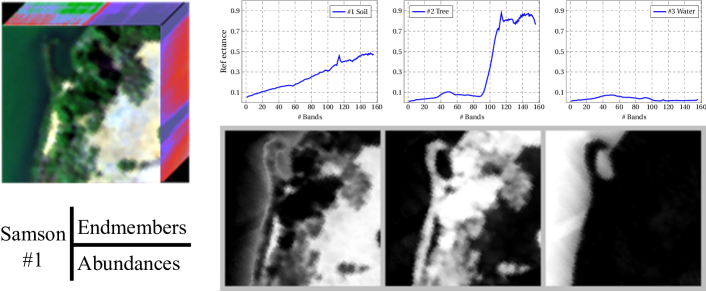
(a) Samson#1 and its 3 endmembers: #1 Soil, #2 Tree and #3 Water.

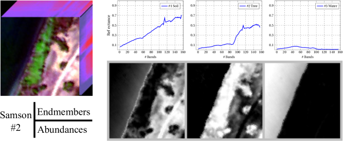
(b) Samson#2 and its 3 endmembers: #1 Soil, #2 Tree and #3 Water.

(c) Samson#3 and its 3 endmembers: #1 Soil, #2 Tree and #3 Water.

Figure 2: The three subimages selected from the Samson hyperspectral image. They are Samson#1, Samson#2 and Samson#3 respectively, as shown in Figs 2a, 2b and 2c. Besides, we provide the illustration of the ground truth endmembers and abundance maps for each subimage.

V Summarization of the 15 Real Hyperspectral Images and their 18 Ground Truths

V-A Samson’s three subimages

The Samson image is illustrated in Fig. 1a, where there are $952\times 952$ pixels [15, 16, 14, 80]. Each pixel is observed at 156 bands covering the electromagnetic spectra from $401\thinspace nm$ to $889\,nm$. As a result, the spectral resolution is highly up to $3.13\,nm$. This data is in good condition and not degraded by the blank channels or badly noised channels. The original image is very large, which could be computationally expensive for the HU study. Accordingly, three subimages are selected due to that they contain large transitional areas which consist of lots of mixed pixels. We name the three ROIs as Samson#1, Samson#2 and Samson#3 respectively for convenience. Please refer to the Fig. 1a and Table I for their information, e.g., their locations, sizes, scenes, number of bands etc.

All of three ROIs have $95\times 95$ pixels. The first ROI (i.e., Samson#1) starts from the $\left(252,\,332\right)$-th pixel in the original image, cf., Figs. 1a and 2a. The top-left pixel in Samson#2 corresponds to the $\left(232,\,93\right)$-th pixel in the original image, cf., Figs. 1a and 2b. Samson#3’s first pixel is the $\left(643,\,455\right)$-th pixel in the Samson image, cf., Figs. 1a and 2c. Specifically, there are three endmembers in this image, i.e., "#1 Soil", "#2 Tree" and "#3 Water" respectively, as shown in Fig. 2.

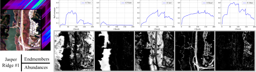
(a) Jasper Ridge#1 and its five endmembers “#1 Road”, “#2 Soil”, “#3 Water”, “#4 Tree” and “#5 Other” respectively.

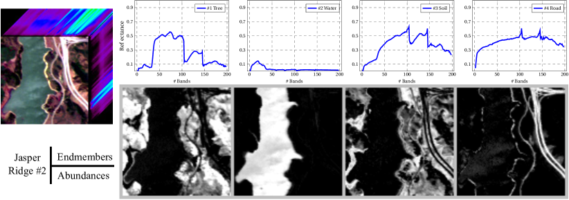
(b) Jasper Ridge#2 and its four endmembers “#1 Road”, “#2 Soil”, “#3 Water” and “#4 Tree” respectively.

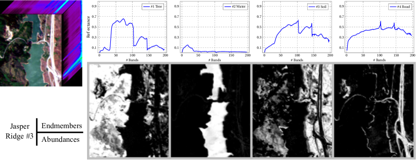
(c) Jasper Ridge#3 and its four endmembers “#1 Road”, “#2 Soil”, “#3 Water” and “#4 Tree” respectively.

Figure 3: The three subimages selected from the Jasper Ridge hyperspectral image. They are Jasper Ridge#1, Jasper Ridge#2 and Jasper Ridge#3 respectively as shown in Figs 3a, 3b and 3c. Besides, we provide the illustration of the endmembers and the abundance maps for each subimage.

V-B Jasper Ridge’s three subimages

Jasper Ridge is a popular hyperspectral image [81, 82], as shown in Fig. 1b. It was captured via the AVIRIS (Airborne Visible/Infrared Imaging Spectrometer) sensor by the Jet Propulsion Laboratory (JPL). The ground sample distance (GSD) is $20\thinspace m$ [82]. There are $512\times 614$ pixels in it. Each pixel is recorded at 224 electromagnetic bands ranging from $380\thinspace nm$ to $2,500\thinspace nm$. The spectral resolution is highly up to $9.46\,nm$. Due to the dense water vapor and atmospheric effects, we remove the spectral bands 1–3, 108–112, 154–166 and 220–224, remaining 198 bands. This is a common preprocessing step if the HU methods do not focus on the robust learning [83, 2, 16, 20, 84, 78].

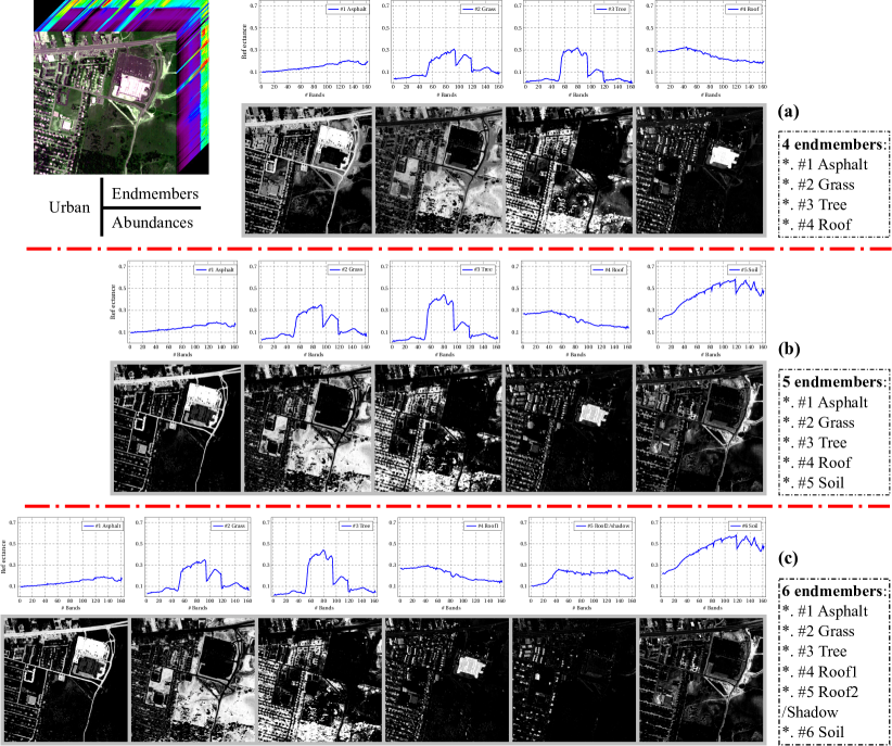
Figure 4: The three versions of ground truths for the Urban hyperspectral image. (a) illustrates the ground truth that has 4 endmembers; (b) shows the ground truth that has 5 endmembers; (c) the ground truth that has 6 endmembers.

Since the full hyperspectral image, as shown in Fig. 1b, is too complex to get the ground truth, we consider three subimages, named as Jasper Ridge#1, Jasper Ridge#2 and Jasper Ridge#3 respectively. Please refer to the Fig. 1b and Table I for their information. The first subimage (i.e., Jasper Ridge#1) consists of $115\times 115$ pixels, whose top-left pixel is the $(1,\thinspace 272)$-th pixel in the original image. There are five endmembers in Jasper Ridge#1, i.e., “#1 Road”, “#2 Soil”, “#3 Water”, “#4 Tree” and “#5 Other”, as shown in Fig. 3a.

Jasper Ridge#2 contains $100\times 100$ pixels. The first pixel is the $\left(105,\,269\right)$-th pixel in the original image. There are four endmembers latent in this subimage: “#1 Road”, “#2 Soil”, “#3 Water” and “#4 Tree”, as shown in Fig. 3b. Since we provided the information of this subimage in the papers [14, 15, 16] and published the data (including the ground truth) on the homepage [85] in 2015, it has been widely used in more than 10 HU papers [82, 86, 30, 87, 31, 88, 89, 90, 2, 91] to verify the state-of-the-art algorithms. The third subimage (i.e., Jasper Ridge#3) consists of $122\times 104$ pixels. The first (i.e., top-left) pixel is the $\left(1,\,246\right)$-th pixel in the original image. There are four endmembers latent in the Jasper Ridge#3: “#1 Road”, “#2 Soil”, “#3 Water” and “#4 Tree”, as shown in Fig. 3c.

V-C HYDICE Urban and its two subimages

HYDICE Urban is one of the most widely used hyperspectral image for the HU research [36, 28, 92, 15, 16, 2, 93, 94, 95, 96, 31, 12, 97]. It was recorded by the HYDICE (Hyperspectral Digital Image Collection Experiment) sensor in October 1995, whose scene is an urban area at Copperas Cove, TX, U.S. There are $307\times 307$ pixels in this image; each pixel corresponds to a $2\times 2\thinspace m^{2}$ region in the scene. The image has 210 spectral bands ranging from $400\thinspace nm$ to $2,500\thinspace nm$, resulting in a very high spectral resolution of $10\thinspace nm$. After removing the badly degraded bands 1–4, 76, 87, 101–111, 136–153 and 198–210 (due to dense water vapor and atmospheric effects), we remain 162 bands. There are three versions of ground truths for the HYDICE Urban hyperspectral image:

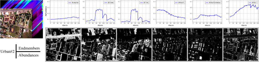
(a) Urban#1 and its six endmembers “#1 Asphalt”, “#2 Grass”, “#3 Tree”, “#4 Roof₁”, “#5 Roof2/shado” and “6 Soil” respectively.

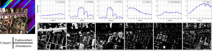
(b) Urban#2 and its six endmembers “#1 Asphalt”, “#2 Grass”, “#3 Tree”, “#4 Roof₁”, “#5 Roof2/shado” and “6 Soil” respectively.

Figure 5: The two challenging subimages selected from the Urban hyperspectral image, i.e., Urban#1 and Urban#2, respectively. Besides, we provide the illustration of the endmembers and their abundance maps for each subimage.

1). In the early HU papers [36, 28, 15, 16, 2, 12, 94, 31], it is widely accepted that there are four endmembers in the HYDICE Urban. They are “#1 Asphalt Road”, “#2 Grass”, “#3 Tree” and “#4 Roof”, as shown in Fig. 4a.

2). Recently, the analyse on Urban image become more and more precise. The “#1 Asphalt Road” is divided into “#1 Asphalt” and “#6 Soil” whereas the “#4 Roof” is divided into “#4 Roof₁” and “#5 Roof₂/shadow”. In other words, the number of endmembers rises to six [12, 97]; they are “#1 Asphalt”, “#2 Grass”, “#3 Tree”, “#4 Roof₁”, “#5 Roof2/shado” and “6 Soil”, as shown in shown in Fig. 4c.

(a) Cuprite

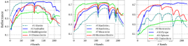
(b) The ground truth endmember spectrum.

Figure 6: (a) is the Cuprite hyperspectral image, which is selected in from the image scene in Fig. 1d, and (b) displays the ground truth endmember spectra.

3). Apart from the above two versions of ground truths, we introduce a new ground truth that consists of 5 endmembers: “#1 Asphalt”, “#2 Grass”, “#3 Tree”, “#4 Roof” and “5 Soil”, as shown in Fig. 4b. Compared with the first version, the “#1 Asphalt Road” is divided into “#1 Asphalt” and “#5 Soil”. Compared with the second version, we merge “#4 Roof₁” and “#5 Roof₂/shadow” into “#4 Roof”.

To make it more challenging, we select two subimages from the Urban image (cf. Fig. 1c). In them, the small objects, like small houses, vehicles and small grasslands etc., are the main scene, causing lots of transitional areas. Such case surely leads to lots of mixed pixels due to the low spatial resolution of hyperspectral sensors. The first subimage (i.e., Urban#1) has $160\times 168$ pixels, whose first pixel is the $\left(1,\,1\right)$-th pixel in the original image. The second subimage (i.e., Urban#2) starts from the $\left(40,\,1\right)$-th pixel in the original image. It also has $160\times 168$ pixels. There are six endmembers: "#1 Asphalt", "#2 Grass", "#3 Tree", “#4 Roof₁”, "#5 Roof2/shadow", and "6 Soil" in both Urban#1 (cf., Fig. 5a) and Urban#2 (cf., Fig. 5b).

V-D Cuprite

Cuprite is the most benchmark and challenging hyperspectral image for the HU research [98, 99, 100, 101, 102, 103, 14, 50, 53, 12, 37, 39], which is captured by the AVIRIS sensor. It covers a Cuprite area in Las Vegas, NV, U.S. There are 224 spectral bands in the Cuprite image, ranging from $370\thinspace nm$ to $2,480\thinspace nm$. After removing the noisy bands (i.e., 1–2 and 221–224) and the water absorption bands (i.e., 104–113 and 148–167), it remains 188 bands. In this paper, a subimage of $250\times 190$ pixels is considered, which is widely used in the state-of-the-art HU papers [39, 12, 50, 14]. Please refer to Fig. 1d for the illustration of its position, image size and scene etc.

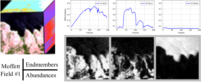
(a) Moffett Field#1 and its three endmembers.

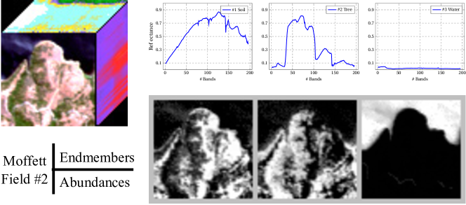
(b) Moffett Field#2 and its three endmembers.

Figure 7: The two subimages selected from the Moffett Field hyperspectral image. They are Moffett Field#1 and Moffett Field#2, respectively, as shown in Figs 7a and 7b. There are 3 endmembers, i.e., “#1 Soil”, “#2 Tree” and “#3 Water” in both subimages. Besides, we provide the illustration of the endmembers and their abundance maps for each subimage.

In this subimage, there are 14 types of minerals (or endmembers), whose spectra can be obtained from the ENVI software. There are very minor differences between the variants of the same type of mineral, for example Kaolinite₁ and Kaolinite₃ are very similar in signature. The researchers have their own thoughts, resulting in different versions of ground truths. In [39], there are 14 endmembers; while there are 10 endmembers in [12]; then Dr. Lu hold that there are 12 endmembers in the Cuprite. Here we agree with Dr. Lu’s setting. Please refer to Fig. 6 for the illustration of the 12 endmembers. Because there are small differences in the setting of endmembers among the papers [50, 53, 12, 37, 39], the results of the state-of-the-art methods in those papers might be different from each other.

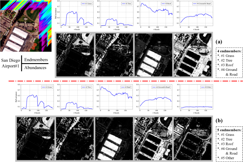
Figure 8: Two versions of HU ground truths for the San Diego Airport hyperspectral image: (a) illustrates the ground truth that has 4 endmembers; (b) shows the ground truth that has 5 endmembers. (best viewed in color)

V-E Moffett Field

The Moffett Field hyperspectral image is illustrated in Fig. 1e. It was captured via the AVIRIS sensor by the JPL in 1997 and was used in a number of state-of-the-art papers [104, 105, 106, 107, 108, 109]. There are $512\times 614$ pixels and 224 spectral bands, ranging the electromagnetic spectra from $400\thinspace nm$ to $2500\thinspace nm$. The spectral resolution is up to $9.38\thinspace nm$. The full image can be found in [110]. It consists of a large area of water (that appears in dark pixel at the top of the image) and a coastal area composed of trees and soil. Due to the water vapor and atmospheric effects, we remove the noisy spectral bands. After this process, there remains 196 bands.

The original image is very large in size and too complex to analyze because the spatial resolution is low and the object is very small in the scene. In this paper, we select two subimages for the HU study. Please refer to Fig.1e for their locations, image sizes and scenes etc. The first subimage (named Moffett Field#1) consists of $60\times 60$ pixels, whose first (top-left) pixel is the $\left(54,\,172\right)$-th pixel in the original image. The second subimage (named Moffett Field#2) also has $60\times 60$ pixels. Its first pixel is the $\left(62,\,146\right)$-th pixel in the full image. A similar subimage with Moffett Field#1 was used in [109, 111], where the authors hold that there are three endmembers. In this paper, we agree with their setting. The three endmembers for both Moffett Field#1 and Moffett Field#2 are “#1 Soil”, “#2 Tree” and “#3 Water”, respectively, as shown in Figs. 7a and 7b.

V-F San Diego Airport

San Diego Airport is a popular airborne hyperspectral image collected by the AVIRIS sensor [76, 112, 113, 114]. There are $400\times 400$ pixels and 224 spectral bands, as illustrated in Fig. 1f. After removing the noisy bands with the water vapor and atmospheric effects, including the bands 1–6, 33–35, 97, 107–113, 153–166, and 221–224, there remains 189 spectral bands. In this paper, we select a subimage for the HU study. It has $160\times 140$ pixels. The top-left pixel is the $\left(241,\,261\right)$-th pixel in the original image, as shown in Fig. 1f. There are two endmember settings: (1) the first setting has 4 endmembers, i.e., “#1 Grass”, “#2 Tree”, “#3 Roof” and “#4 Ground & Road”, as shown in Fig. 8a; (2) the second setting has 5 endmembers, i.e., “#1 Grass”, “#2 Tree”, “#3 Roof”, “#4 Ground & Road” and “#5 Other”, as shown in Fig. 8b.

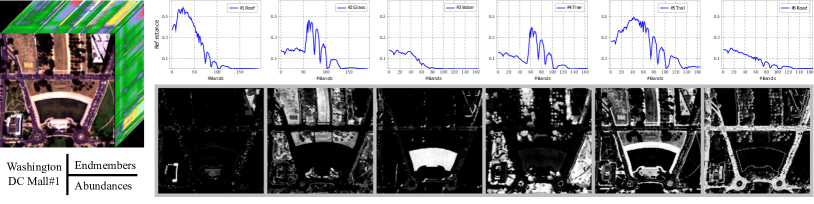
(a) WDM#1 and its six endmembers.

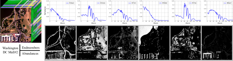
(b) WDM#2 and its six endmembers.

Figure 9: Two challenging subimages selected from the Washington DC Mall image: WDM#1 and WDM#2 as shown in Figs 9a and 9b. For each subimage, we give the illustration of the ground truth endmembers and abundances.

V-G Washington DC Mall (WDM)

The Washington DC Mall (i.e., WDM), an airborne hyperspectral image flightline over the Washington DC Mall (cf. Fig. 9g), is used to verify a lot of research works [115, 31, 102, 28, 116, 37]. It was collected by the HYDICE sensor. The full image can be downloaded from the webpage. There are $1208\times 307$ pixels and $210$ spectral channels, covering the the electromagnetic spectra from $400\thinspace nm$ to $2400\thinspace nm$. The spectral resolution is up to $9.52\thinspace nm$. After removing the bands with water vapor and atmospheric effects, including 103–106, 138–148, and 207–210, there remains 191 bands [102].

In this paper, we select two subimages for the HU study, i.e., WDM#1 and WDM#2 respectively. Please refer to Fig. 9g and Table I for their information like locations and scenes etc. The first subimage (i.e. WDM#1) has $150\times 150$ pixels, whose first pixel starts from the $\left(549,\,160\right)$-th pixel in the original image. WDM#1 has been used in [37], where they provide the rough locations of the six endmember; however, they did not share the ground truth on the Internet. The six endmembers are “#1 Roof”, “#2 Grass”, “#3 Water”, “#4 Tree”, “#5 Trail” and “#6 Road” respectively, as shown in Fig. 9a. The second subimage (i.e. WDM#2) has $180\times 160$ pixels, whose left-top pixel is the $\left(945,\,90\right)$-th pixel in the original image. The six endmembers are “#1 Road”, “#2 Grass”, “#3 Trail”, “#4 Water”, “#5 Tree” and “#6 Roof” respectively, as shown in Fig. 9b.

VI The Simulated Hyperspectral Image

This section provides the method to generate a complex synthetic image [27, 28, 2, 12, 29, 30, 31, 32] for the HU research. It consists of two steps. First, 15 true spectra are chosen from the United States Geological Survey (USGS) digital spectral library as the candidate endmembers. Their signature are shown in Fig. 10. The first $K$ spectra are selected as the true endmember, where $2\leq K\leq 15$ is the number of endmembers.

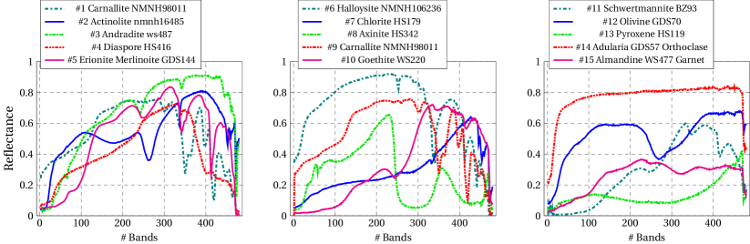
Figure 10: The signature of 15 candidate endmembers used for the simulation of hyperspectral images. Each signature is observed at 480 spectral bands.

Second, we use the method in [27, 28, 2, 12, 30, 32] to generate the abundance maps, which has the following steps:

1). We divide an image of $z^{2}\times z^{2}\mbox{$\left(z\in\mathbb{Z}^{+}\right)$}$ pixels into $z\times z$ regions. The default setting is $z=8$.

2). Each region is filled up with a type of ground cover, which means the abundance of that endmember is 1 in the whole region. Note that, this process is randomly implemented.

3). To generate the mixed pixels, we use the $\left(z+1\right)\times\left(z+1\right)$ spatial low-pass filter. Such process causes large transitional areas, where there are lots of mixed pixels.

4). To remove pure pixels and generate sparse abundances, we replace the pixels whose largest abundance is larger than 0.8 with a mixture of two endmembers with equal abundances.

Now both endmembers $\widehat{\mathbf{M}}$ and abundances $\widehat{\mathbf{A}}$ have been generated. Based on them, a perfect hyperspectral image is created as $\widehat{\mathbf{Y}}=\widehat{\mathbf{M}}\widehat{\mathbf{A}}$. To simulate a more real remote sensing image that contains complex noises, we add the zero-mean Gaussian (or some other) noise to the generate the image data. The Signal-to-Noise Ratio (SNR) is defined as follows:

$$\text{SNR}=10\log_{10}\left\{\frac{\mathbb{E}\left[\mathbf{y}^{\top}\mathbf{y}\right]}{\mathbb{E}\left[\mathbf{n}^{\top}\mathbf{n}\right]}\right\}.$$ (20)

With the above synthetic hyperspectral image, we can verify the HU algorithmss from the following four perspectives:

• Robustness analysis to the noise corruptions, e.g., $\text{SNR$\in\left\{\infty,35,\cdots,10\thinspace\text{dB}\right\}$ }.$

• Generalization to the pixel number, which is set by $z$.

• Robustness to the endmember number $\left\{K\!\mid\!2\!\leq\!K\!\leq\!15\right\}$.

• Generalization to the number of bands in the image.

We will provide the full codes for this simulated dataset.

TABLE II: The performances of five benchmark HU algorithms on the Samson#1, Samson#2 and Samson#3 hyperspectral images.

Samson #1	Endmembers	Spectral Angle Distance (SAD)					Root Mean Square Error (RMSE)
		VCA	NMF	$\ell_{1}$-NMF	$\ell_{1/2}$-NMF	G-NMF	VCA	NMF	$\ell_{1}$-NMF	$\ell_{1/2}$-NMF	G-NMF
	#1 Soil	0.1531	0.0861	0.0582	0.0902	0.0529	0.1765	0.1110	0.0930	0.0990	0.0993
	#2 Tree	0.0487	0.0556	0.0545	0.0410	0.0576	0.1372	0.0886	0.0798	0.0919	0.0734
	#3 Water	0.1296	0.1560	0.1233	0.0410	0.1609	0.1748	0.0757	0.0511	0.0344	0.0750
	Avg.	0.1105	0.0992	0.0787	0.0574	0.0905	0.1628	0.0918	0.0746	0.0751	0.0826
Samson #2	Endmembers	Spectral Angle Distance (SAD)					Root Mean Square Error (RMSE)
		VCA	NMF	$\ell_{1}$-NMF	$\ell_{1/2}$-NMF	G-NMF	VCA	NMF	$\ell_{1}$-NMF	$\ell_{1/2}$-NMF	G-NMF
	#1 Soil	0.4239	0.2793	0.1780	0.2074	0.2647	0.1504	0.1633	0.1425	0.1719	0.1583
	#2 Tree	0.1118	0.1150	0.0542	0.0559	0.1161	0.1483	0.1710	0.1341	0.1683	0.1663
	#3 Water	0.0662	0.0804	0.0778	0.0731	0.0821	0.1055	0.0610	0.0360	0.0395	0.0610
	Avg.	0.2006	0.1582	0.1033	0.1121	0.1543	0.1347	0.1318	0.1042	0.1266	0.1285
Samson #3	Endmembers	Spectral Angle Distance (SAD)					Root Mean Square Error (RMSE)
		VCA	NMF	$\ell_{1}$-NMF	$\ell_{1/2}$-NMF	G-NMF	VCA	NMF	$\ell_{1}$-NMF	$\ell_{1/2}$-NMF	G-NMF
	#1 Soil	0.0454	0.0422	0.0315	0.0316	0.0509	0.0801	0.0792	0.0326	0.0498	0.0870
	#2 Tree	0.0600	0.0714	0.0425	0.0429	0.0781	0.0771	0.0802	0.0319	0.0427	0.0895
	#3 Water	0.1134	0.1155	0.1129	0.1135	0.1158	0.0217	0.0263	0.0072	0.0134	0.0321
	Avg.	0.0729	0.0764	0.0623	0.0627	0.0816	0.0596	0.0619	0.0239	0.0353	0.0695

TABLE III: The SAD performances of five benchmark HU algorithms on the Cuprite hyperspectral images.

Endmembers	Spectral Angle Distance (SAD)
	VCA	NMF	$\ell_{1}$-NMF	$\ell_{1/2}$-NMF	G-NMF
#1 Alunite	0.1584	0.1640	0.1618	0.1458	0.1632
#2 Andradite	0.0773	0.1166	0.1253	0.0783	0.1279
#3 Buddingtonite	0.0999	0.1343	0.1391	0.1456	0.1406
#4 Dumortierite	0.1033	0.1202	0.1212	0.1067	0.1211
#5 Kaolinite1	0.0892	0.1042	0.0951	0.1004	0.1001
#6 Kaolinite2	0.0682	0.1120	0.1024	0.0763	0.1125
#7 Muscovite	0.1912	0.2440	0.2490	0.2228	0.2489
#8 Montmorillonite	0.0721	0.1165	0.0980	0.0769	0.1209
#9 Nontronite	0.0784	0.1115	0.1036	0.0940	0.1232
#10 Pyrope	0.0907	0.0966	0.0935	0.0831	0.1045
#11 Sphene	0.0702	0.0952	0.0903	0.0788	0.0923
#12 Chalcedony	0.0870	0.1811	0.1719	0.1542	0.1513
Avg.	0.0988	0.1330	0.1293	0.1136	0.1339

TABLE IV: The performances of five benchmark HU algorithms on the HYDICE Urban image, which has three versions of ground truths.

V1: 4 endmembers	Endmembers	Spectral Angle Distance (SAD)					Root Mean Square Error (RMSE)
		VCA	NMF	$\ell_{1}$-NMF	$\ell_{1/2}$-NMF	G-NMF	VCA	NMF	$\ell_{1}$-NMF	$\ell_{1/2}$-NMF	G-NMF
	#1 Asphalt	0.2152	0.2114	0.1548	0.1349	0.2086	0.2884	0.2041	0.2279	0.3225	0.2056
	#2 Grass	0.3547	0.3654	0.2876	0.0990	0.3716	0.3830	0.2065	0.2248	0.3387	0.2078
	#3 Tree	0.2115	0.1928	0.0911	0.0969	0.1934	0.2856	0.1870	0.1736	0.2588	0.1824
	#4 Roof	0.7697	0.7370	0.7335	0.5768	0.7377	0.1638	0.1395	0.1861	0.1782	0.1389
	Avg.	0.3877	0.3767	0.3168	0.2269	0.3778	0.2802	0.1843	0.2031	0.2746	0.1837
V2: 5 endmembers	Endmembers	Spectral Angle Distance (SAD)					Root Mean Square Error (RMSE)
		VCA	NMF	$\ell_{1}$-NMF	$\ell_{1/2}$-NMF	G-NMF	VCA	NMF	$\ell_{1}$-NMF	$\ell_{1/2}$-NMF	G-NMF
	#1 Asphalt	0.3009	0.3284	0.1664	0.1837	0.3502	0.2898	0.2941	0.3080	0.3408	0.2944
	#2 Grass	0.3547	0.4575	0.1826	0.1143	0.5539	0.3634	0.3417	0.2048	0.3099	0.3823
	#3 Tree	0.4694	0.2337	0.1335	0.0658	0.2402	0.3092	0.2513	0.1245	0.2944	0.2887
	#4 Roof	0.4066	0.4134	0.4801	0.0834	0.4340	0.2202	0.1548	0.1101	0.1751	0.1581
	#5 Soil	1.0638	1.0478	1.0948	0.0290	0.9651	0.2791	0.2755	0.2797	0.3125	0.2796
	Avg.	0.5191	0.4962	0.4115	0.0952	0.5087	0.2923	0.2635	0.2054	0.2865	0.2806
V3: 6 endmembers	Endmembers	Spectral Angle Distance (SAD)					Root Mean Square Error (RMSE)
		VCA	NMF	$\ell_{1}$-NMF	$\ell_{1/2}$-NMF	G-NMF	VCA	NMF	$\ell_{1}$-NMF	$\ell_{1/2}$-NMF	G-NMF
	#1 Asphalt	0.2441	0.3322	0.2669	0.3092	0.3274	0.2555	0.2826	0.2803	0.3389	0.2787
	#2 Grass	0.3058	0.4059	0.3294	0.0792	0.3787	0.2696	0.3536	0.2937	0.2774	0.3184
	#3 Tree	0.6371	0.2558	0.2070	0.0623	0.2629	0.3212	0.2633	0.1859	0.2701	0.2404
	#4 Roof1	0.2521	0.3701	0.4370	0.0680	0.3264	0.2500	0.1662	0.1358	0.1541	0.1725
	#5 Roof2/	0.7451	0.6223	0.5330	0.1870	0.6831	0.2157	0.1603	0.2136	0.1660	0.1441
	Shadow
	#6 Soil	1.1061	0.9978	1.0371	0.0287	0.9859	0.2714	0.2505	0.2594	0.3542	0.2547
	Avg.	0.5484	0.4974	0.4684	0.1224	0.4941	0.2639	0.2461	0.2281	0.2601	0.2348

TABLE V: The performances of five benchmark HU algorithms on the Urban#1 and Urbann#2 hyperspectral sub-images.

Urban #1	Endmembers	Spectral Angle Distance (SAD)					Root Mean Square Error (RMSE)
		VCA	NMF	$\ell_{1}$-NMF	$\ell_{1/2}$-NMF	G-NMF	VCA	NMF	$\ell_{1}$-NMF	$\ell_{1/2}$-NMF	G-NMF
	#1 Asphalt	0.2166	0.3172	0.1843	0.2761	0.3273	0.2962	0.2544	0.2663	0.2475	0.2488
	#2 Grass	1.3196	0.5520	1.1585	0.6055	0.4975	0.4199	0.2727	0.3864	0.2982	0.2720
	#3 Tree	0.1696	0.1221	0.0708	0.1034	0.1188	0.1934	0.1648	0.2271	0.1602	0.1709
	#4 Roof1	0.2475	0.3403	0.3632	0.3537	0.3686	0.3176	0.1871	0.1411	0.1782	0.1695
	#5 Roof2/	0.9453	0.6446	0.3751	0.6482	0.6075	0.1965	0.1957	0.2693	0.2080	0.2020
	Shadow
	#6 Soil	0.3329	0.4991	0.2179	0.4191	0.4560	0.2409	0.2661	0.2509	0.2843	0.2696
	Avg.	0.5386	0.4125	0.3950	0.4010	0.3959	0.2774	0.2235	0.2568	0.2294	0.2222
Urban #2	Endmembers	Spectral Angle Distance (SAD)					Root Mean Square Error (RMSE)
		VCA	NMF	$\ell_{1}$-NMF	$\ell_{1/2}$-NMF	G-NMF	VCA	NMF	$\ell_{1}$-NMF	$\ell_{1/2}$-NMF	G-NMF
	#1 Asphalt	0.2112	0.2693	0.2319	0.4158	0.2874	0.2724	0.2710	0.2617	0.4366	0.2488
	#2 Grass	1.2238	0.2990	0.3400	0.2348	0.3526	0.3673	0.2341	0.2662	0.2809	0.2430
	#3 Tree	0.1778	0.1263	0.1203	0.1037	0.1212	0.1910	0.1636	0.1776	0.2120	0.1732
	#4 Roof1	0.2012	0.4419	0.4462	0.4320	0.4304	0.3693	0.1360	0.1239	0.1341	0.1359
	#5 Roof2/	1.0188	0.5260	0.5151	0.3300	0.5371	0.1857	0.2244	0.2249	0.2448	0.2030
	Shadow
	#6 Soil	0.4134	0.5414	0.4434	0.0786	0.5253	0.2235	0.2619	0.2675	0.4651	0.2535
	Avg.	0.5410	0.3673	0.3495	0.2658	0.3757	0.2682	0.2152	0.2203	0.2956	0.2096

TABLE VI: The HU results of five benchmark HU algorithms on the JasperRidge#1, JasperRidge#2 and JasperRidge#3 hyperspectral images.

Jasper Ridge #1	Endmembers	Spectral Angle Distance (SAD)					Root Mean Square Error (RMSE)
		VCA	NMF	$\ell_{1}$-NMF	$\ell_{1/2}$-NMF	G-NMF	VCA	NMF	$\ell_{1}$-NMF	$\ell_{1/2}$-NMF	G-NMF
	#1 Tree	0.3381	0.1325	0.0553	0.0458	0.0743	0.2651	0.1327	0.0928	0.1032	0.0752
	#2 Water	0.2573	0.2823	0.0300	0.0303	0.2923	0.2711	0.1384	0.0714	0.0911	0.1366
	#3 Soil	0.3062	0.2125	0.1318	0.0534	0.2005	0.2567	0.2221	0.2536	0.2631	0.1837
	#4 Road	0.6053	0.4843	0.6352	0.5525	0.5411	0.2361	0.1876	0.2064	0.2389	0.1908
	#5 Other	0.7156	0.6463	1.0503	0.8187	0.6742	0.2842	0.1601	0.1357	0.1451	0.1669
	Avg.	0.4445	0.3516	0.3805	0.3001	0.3565	0.2626	0.1682	0.1520	0.1683	0.1506
Jasper Ridge #2	Endmembers	Spectral Angle Distance (SAD)					Root Mean Square Error (RMSE)
		VCA	NMF	$\ell_{1}$-NMF	$\ell_{1/2}$-NMF	G-NMF	VCA	NMF	$\ell_{1}$-NMF	$\ell_{1/2}$-NMF	G-NMF
	#1 Tree	0.2565	0.2130	0.0680	0.0409	0.2781	0.3268	0.1402	0.0636	0.0707	0.1740
	#2 Water	0.2474	0.2001	0.3815	0.1682	0.2530	0.3151	0.1106	0.0660	0.1031	0.1375
	#3 Soil	0.3584	0.1569	0.0898	0.0506	0.3246	0.2936	0.2557	0.2463	0.2679	0.2840
	#4 Road	0.5489	0.3522	0.4118	0.3670	0.2776	0.2829	0.2450	0.2344	0.2737	0.2279
	Avg.	0.3528	0.2305	0.2378	0.1567	0.2833	0.3046	0.1879	0.1526	0.1789	0.2058
Jasper Ridge #3	Endmembers	Spectral Angle Distance (SAD)					Root Mean Square Error (RMSE)
		VCA	NMF	$\ell_{1}$-NMF	$\ell_{1/2}$-NMF	G-NMF	VCA	NMF	$\ell_{1}$-NMF	$\ell_{1/2}$-NMF	G-NMF
	#1 Tree	0.1168	0.0992	0.0969	0.1081	0.1117	0.1522	0.1000	0.1182	0.1017	0.1164
	#2 Water	0.2763	0.3124	0.0513	0.0474	0.3369	0.1467	0.1248	0.0418	0.0651	0.1298
	#3 Soil	0.5364	0.3748	0.3525	0.2419	0.3414	0.2475	0.2663	0.2536	0.2289	0.2247
	#4 Road	0.4235	0.2997	0.3906	0.4098	0.2200	0.2105	0.2163	0.1707	0.1834	0.1688
	Avg.	0.3383	0.2715	0.2228	0.2018	0.2525	0.1892	0.1769	0.1461	0.1448	0.1599

TABLE VII: The performances of five benchmark HU algorithms on the Moffett Field#1 and Moffett Field#2 hyperspectral images.

Moffett Field#1	Endmembers	Spectral Angle Distance (SAD)					Root Mean Square Error (RMSE)
		VCA	NMF	$\ell_{1}$-NMF	$\ell_{1/2}$-NMF	G-NMF	VCA	NMF	$\ell_{1}$-NMF	$\ell_{1/2}$-NMF	G-NMF
	#1 Soil	0.0760	0.0475	0.0884	0.0717	0.1006	0.2492	0.0923	0.0912	0.0943	0.1085
	#2 Tree	0.0418	0.0432	0.0332	0.0357	0.0477	0.0992	0.0540	0.0595	0.0590	0.0842
	#3 Water	0.3946	0.3528	0.3471	0.3432	0.3697	0.2751	0.1006	0.0790	0.0839	0.1219
	Avg.	0.1708	0.1478	0.1563	0.1502	0.1727	0.2078	0.0823	0.0766	0.0791	0.1049
Moffett Field#2	Endmembers	Spectral Angle Distance (SAD)					Root Mean Square Error (RMSE)
		VCA	NMF	$\ell_{1}$-NMF	$\ell_{1/2}$-NMF	G-NMF	VCA	NMF	$\ell_{1}$-NMF	$\ell_{1/2}$-NMF	G-NMF
	#1 Soil	0.0509	0.0398	0.0360	0.0258	0.0402	0.1120	0.1685	0.0456	0.0703	0.1701
	#2 Tree	0.0406	0.0419	0.0684	0.0592	0.0422	0.0403	0.0600	0.0286	0.0417	0.0595
	#3 Water	0.2793	0.3224	0.0555	0.0726	0.3247	0.1072	0.1771	0.0348	0.0501	0.1779
	Avg.	0.1236	0.1347	0.0533	0.0525	0.1357	0.0865	0.1352	0.0364	0.0540	0.1359

TABLE VIII: The HU results of five benchmark algorithms on the WDM#1 and WDM#2 subimages. WDM denotes Washington DC Mall.

WDM #1	Endmembers	Spectral Angle Distance (SAD)					Root Mean Square Error (RMSE)
		VCA	NMF	$\ell_{1}$-NMF	$\ell_{1/2}$-NMF	G-NMF	VCA	NMF	$\ell_{1}$-NMF	$\ell_{1/2}$-NMF	G-NMF
	#1 Roof	0.18175	0.23343	0.24818	0.22110	0.21093	0.12021	0.16432	0.16577	0.16744	0.17293
	#2 Grass	0.24779	0.16813	0.17883	0.17013	0.17285	0.18837	0.19286	0.19132	0.19167	0.19202
	#3 Water	0.18327	0.17505	0.16717	0.17077	0.17099	0.33159	0.20351	0.20051	0.20236	0.19769
	#4 Tree	0.13241	0.15310	0.15853	0.14407	0.15898	0.15137	0.14405	0.14417	0.14449	0.14406
	#5 Trail	0.17445	0.26442	0.26116	0.26343	0.27032	0.30302	0.26970	0.27523	0.27606	0.28636
	#6 Road	0.42313	0.35212	0.34244	0.37354	0.36481	0.36034	0.29809	0.29570	0.30967	0.29885
	Avg.	0.22380	0.22437	0.22605	0.22384	0.22481	0.24248	0.21209	0.21212	0.21528	0.21532
WDM #2	Endmembers	Spectral Angle Distance (SAD)					Root Mean Square Error (RMSE)
		VCA	NMF	$\ell_{1}$-NMF	$\ell_{1/2}$-NMF	G-NMF	VCA	NMF	$\ell_{1}$-NMF	$\ell_{1/2}$-NMF	G-NMF
	#1 Asphalt	0.72505	0.81097	0.70794	0.75846	0.83643	0.33940	0.33944	0.33806	0.34125	0.34041
	#2 Grass	1.17554	1.41735	0.07486	1.17832	1.44942	0.45647	0.46033	0.33928	0.44229	0.46026
	#3 Tree	0.98158	0.69179	0.11641	0.14168	0.63707	0.21752	0.18320	0.23490	0.21929	0.18256
	#4 Roof1	0.15295	0.04880	0.03986	0.03278	0.04388	0.24413	0.25255	0.25370	0.26166	0.25228
	#5 Roof2/	0.18843	0.09550	1.18046	0.31077	0.08978	0.35982	0.38600	0.26782	0.35865	0.38359
	Shadow
	#6 Soil	0.22996	0.73903	0.80175	0.93171	0.73604	0.26711	0.18963	0.16798	0.16017	0.18300
	Avg.	0.57558	0.63391	0.48688	0.55895	0.63210	0.31408	0.30186	0.26696	0.29722	0.30035

TABLE IX: The performances of five benchmark HU algorithms on the San Diego Aiport image, which has two versions of ground truths.

V1: 4 endmembers	Endmembers	Spectral Angle Distance (SAD)					Root Mean Square Error (RMSE)
		VCA	NMF	$\ell_{1}$-NMF	$\ell_{1/2}$-NMF	G-NMF	VCA	NMF	$\ell_{1}$-NMF	$\ell_{1/2}$-NMF	G-NMF
	#1 Grass	1.0476	0.7738	0.1811	0.0474	0.7763	0.3164	0.3403	0.2675	0.2692	0.3255
	#2 Tree	0.1891	0.1904	0.7613	0.8001	0.1709	0.2257	0.2338	0.2672	0.2851	0.2336
	#3 Roof	0.3844	0.5240	0.4924	0.4608	0.5224	0.4508	0.3361	0.3101	0.3491	0.3348
	#4 Ground	0.2187	0.2543	0.1313	0.0609	0.2487	0.3719	0.2593	0.2283	0.2964	0.2562
	/Road
	Avg.	0.4600	0.4356	0.3915	0.3423	0.4296	0.3412	0.2924	0.2683	0.2999	0.2875
V2: 5 endmembers	Endmembers	Spectral Angle Distance (SAD)					Root Mean Square Error (RMSE)
		VCA	NMF	$\ell_{1}$-NMF	$\ell_{1/2}$-NMF	G-NMF	VCA	NMF	$\ell_{1}$-NMF	$\ell_{1/2}$-NMF	G-NMF
	#1 Grass	0.4806	0.3382	0.3560	0.2957	0.2544	0.3249	0.2916	0.2964	0.2754	0.2906
	#2 Tree	0.1592	0.1361	0.1439	0.1624	0.1430	0.2209	0.2267	0.2212	0.2176	0.2207
	#3 Roof	0.6239	0.6509	0.6293	0.6205	0.6409	0.3299	0.2538	0.2626	0.2715	0.2563
	#4 Ground	0.2509	0.2276	0.2200	0.2047	0.2501	0.3443	0.2544	0.2622	0.2566	0.2581
	/Road
	#5 Other	0.4856	0.5421	0.5586	0.5861	0.6157	0.3382	0.2665	0.2735	0.2781	0.2696
	Avg.	0.4000	0.3790	0.3815	0.3739	0.3808	0.3117	0.2586	0.2632	0.2599	0.2591

VII Experiments Results of 5 Benchmark HU methods on the 18 Hyperspectral Images

In this section, we compare 5 benchmarks HU methods on the 15 hyperspectral images summarized in Section V. The selected 5 methods are widely compared against the state-of-the-art HU methods. The aim is to provide benchmark HU results, saving other’s effort to evaluate their new HU methods.

VII-A Five Benchmark Methods Compared in this Section

1). Vertex Component Analysis [39] (VCA) is a classic geometric method. The code is available on http://www.lx.it.pt/bioucas/code.htm.

2). Nonnegative Matrix Factorization [51] (NMF) is a benchmark statistical method. The code is obtained from http://www.cs.helsinki.fi/u/phoyer/software.html.

3). Nonnegative sparse coding [62] ($\ell_{1}$-NMF) is a classic sparse regularized NMF method. The code is download from http://www.cs.helsinki.fi/u/phoyer/software.html.

4). $\ell_{1/2}$ sparsity-constrained NMF [12] ($\ell{}_{\text{1/2}}$-NMF) is a state-of-the-art method that could get sparser results than $\ell_{1}$-NMF. Since the code is unavailable, we implement it.

5). Graph regularized NMF [64, 61] (G-NMF) is an interesting algorithm that transfers graph information inherent in the hyperspectral image into the abundance space.

We will share the code for all the above five algorithms.

VII-B Experiment Settings and Experiment Results

Generally, there are one or two hyper-parameters in the 5 benchmark methods. We use the coarse to fine grid search method to find the best hyper-parameters [15, 16, 14]. The initialization of the endmembers $\mathbf{M}$ and abundances $\mathbf{A}$ is very important to the final HU results [37]. We employ the same benchmark algorithm, i.e., VCA [39], to initialize $\mathbf{M}$ and $\mathbf{A}$ for the five methods on all the 15 datasets. There are two advantages: (1) it is helpful to generate the reproducible results by the VCA; (2) VCA is really simple, effective and solid.

Two evaluation metrics are used to obtain the quantitative comparison results: (1) the Spectral Angle Distance (SAD) [63, 53, 15, 16, 14] is used to verify the performance of the estimated endmembers; (2) the Root Mean Square Error (RMSE) [12, 15, 117, 16, 14] is for the evaluation of the estimated abundances. To get a valid results, each experiment is repeated 50 times and the mean result is provided in the Tables II, III, V, V, VI, VII, VIII, IX. In short, we summarize the tables that display the results on all the 15 datasets:

1). Table II summarizes the experiment results of all the five benchmark algorithms (reviewed in Section VII-A). There are three tables, displaying the HU results on the three subimages, i.e., Samson#1, Samson#2 and Samson#3 respectively.

2). In Table III, the HU results on the Cuprite image are summarized. Note that the ground truth abundance is not available; only the endmember results are compared.

3). Table V illustrates the HU results of 5 benchmark algorithms on the full HYDICE Urban image. There are 3 versions of ground truths for the Urban images. Accordingly, we summarize 3 versions of HU results in the 3 sub-tables.

4). In Table V, the HU results on the two subimages, Urban#1 and Urban#2, are summarized. There are six endmembers as shown in the Table V.

5). In Table VI, the experiment results on the 3 subimages from the JasperRidge is displayed. The 3 subimage are JasperRidge#1, JasperRidge#2 and JasperRidge#3.

6). Table VII illustrates the HU results on the 2 subimags selected from Moffett Field. They are Moffett Field#1 and Moffett Field#2 respectively as shown in the Table.

7). Table VIII illustrates the HU results on the 2 subimags selected from the Washington DC Mall. They are WDM#1 and WDM#2 respectively.

8). Table IX displays the HU results on the two versions of ground truths on the San Diego Airport dataset.

VIII Conclusion

Hyperspectral unmixing (HU) is an important preprocessing step for a great number of hyperpsectral applications. To promote the HU research, we accomplished this paper by emphasizing on the generation of standard HU datasets (with ground truths) and the summarization of benchmark results of the state-of-the-art HU algorithms. Specifically, this is the first paper to propose a general labeling method for the HU. Via it, we summarized and labeled up to 15 hyperpsectral images. To further enrich the HU datasets, an interesting method has been proposed to transform the hyperspectral classification datasets for the HU research. Besides, we reviewed and implemented a widely accepted algorithm to generate a very complex simulated hyperpsectral image for the HU study. Such synthetic dataset is helpful to verify the HU algorithms under four different conditions.

To summarize the benchmark HU results, we reviewed up to 10 state-of-the-art HU algorithms, and selected the five most benchmark HU algorithms for the comparison. Those HU algorithms are compared on the 15 hyperpsectral images. To the best of our knowledge, this is the first paper to compare the benchmark algorithms on so many real hyperpsectral images. The experient results on this paper may provide a valid baseline for the evaluation of new HU algorithms.

References

- [1] J. Bioucas-Dias and A. Plaza, “Hyperspectral unmixing overview: Geometrical, statistical, and sparse regression-based approaches,” IEEE Journal of Selected Topics in Applied Earth Observations and Remote Sensing, vol. 5, no. 2, pp. 354 –379, april 2012.
- [2] Y. Wang, C. Pan, S. Xiang, and F. Zhu, “Robust hyperspectral unmixing with correntropy-based metric,” IEEE Transactions on Image Processing, vol. 24, no. 11, pp. 4027–4040, 2015.
- [3] R. Kawakami, J. Wright, Y.-W. Tai, Y. Matsushita, M. Ben-Ezra, and K. Ikeuchi, “High-resolution hyperspectral imaging via matrix factorization,” IEEE Conference on Computer Vision and Pattern Recognition, vol. 0, pp. 2329–2336, 2011.
- [4] C. Lanaras, E. Baltsavias, and K. Schindler, “Hyperspectral super-resolution by coupled spectral unmixing,” in IEEE International Conference on Computer Vision, 2015, pp. 3586–3594.
- [5] W. Dong, F. Fu, G. Shi, X. Cao, J. Wu, G. Li, and X. Li, “Hyperspectral image super-resolution via non-negative structured sparse representation,” IEEE Transactions on Image Processing, vol. 25, no. 5, pp. 2337–2352, 2016.
- [6] C. Ma, X. Cao, X. Tong, Q. Dai, and S. Lin, “Acquisition of high spatial and spectral resolution video with a hybrid camera system,” International journal of computer vision, vol. 110, no. 2, pp. 141–155, 2014.
- [7] N. Akhtar, F. Shafait, and A. Mian, “Sparse spatio-spectral representation for hyperspectral image super-resolution,” in European Conference on Computer Vision. Springer, 2014, pp. 63–78.
- [8] ——, “Bayesian sparse representation for hyperspectral image super resolution,” in IEEE Conference on Computer Vision and Pattern Recognition, 2015, pp. 3631–3640.
- [9] Z. Guo, T. Wittman, and S. Osher, “L1 unmixing and its application to hyperspectral image enhancement,” in Defense, Security, and Sensing, ser. Society of Photo-Optical Instrumentation Engineers (SPIE) Conference Series, vol. 7334, no. 1. The International Society for Optical Engineering., Apr. 2009, p. 73341M.
- [10] K. C. Mertens, L. P. C. Verbeke, E. I. Ducheyne, and R. R. D. Wulf, “Using genetic algorithms in sub-pixel mapping,” International Journal of Remote Sensing (IJRS), vol. 24, no. 21, pp. 4241–4247, 2003.
- [11] C. Li, T. Sun, K. Kelly, and Y. Zhang, “A compressive sensing and unmixing scheme for hyperspectral data processing,” IEEE Transactions on Image Processing (TIP), vol. 21, no. 3, pp. 1200–1210, March 2012.
- [12] Y. Qian, S. Jia, J. Zhou, and A. Robles-Kelly, “Hyperspectral unmixing via sparsity-constrained nonnegative matrix factorization,” IEEE Transactions on Geoscience and Remote Sensing, vol. 49, no. 11, pp. 4282 –4297, nov 2011.
- [13] S. Cai, Q. Du, and R. Moorhead, “Hyperspectral imagery visualization using double layers,” IEEE Transactions on Geoscience and Remote Sensing (TGRS), vol. 45, no. 10, pp. 3028–3036, Oct 2007.
- [14] F. Zhu, Y. Wang, B. Fan, S. Xiang, G. Meng, and C. Pan, “Spectral unmixing via data-guided sparsity,” IEEE Transactions on Image Processing (TIP), vol. 23, no. 12, pp. 5412–5427, Dec 2014.
- [15] F. Zhu, Y. Wang, S. Xiang, B. Fan, and C. Pan, “Structured sparse method for hyperspectral unmixing,” ISPRS Journal of Photogrammetry and Remote Sensing, vol. 88, no. 0, pp. 101–118, 2014.
- [16] F. Zhu, Y. Wang, B. Fan, G. Meng, and C. Pan, “Effective spectral unmixing via robust representation and learning-based sparsity,” CoRR, vol. abs/1409.0685, 2014. [Online]. Available: http://arxiv.org/abs/1409.0685
- [17] G. Cheng, Y. Wang, Y. Gong, F. Zhu, and C. Pan, “Urban road extraction via graph cuts based probability propagation,” in Image Processing (ICIP), 2014 IEEE International Conference on. IEEE, 2014, pp. 5072–5076.
- [18] G. Cheng, Y. Wang, F. Zhu, and C. Pan, “Road extraction via adaptive graph cuts with multiple features,” in Image Processing (ICIP), IEEE International Conference on. IEEE, 2015, pp. 3962–3966.
- [19] G. Cheng, F. Zhu, S. Xiang, Y. Wang, and C. Pan, “Accurate urban road centerline extraction from vhr imagery via multiscale segmentation and tensor voting,” Neurocomputing, vol. 205, pp. 407–420, 2016.
- [20] ——, “Semisupervised hyperspectral image classification via discriminant analysis and robust regression,” IEEE J. of Selected Topics in Applied Earth Observations and Remote Sensing, vol. 9, no. 2, pp. 595–608, 2016.
- [21] G. Cheng, F. Zhu, S. Xiang, and C. Pan, “Road centerline extraction via semisupervised segmentation and multidirection nonmaximum suppression,” IEEE Geoscience and Remote Sensing Letters, vol. 13, no. 4, pp. 545–549, 2016.
- [22] J. Yao, X. Zhu, F. Zhu, and J. Huang, “Deep correlational learning for survival prediction from multi-modality datay,” in International Conference on Medical Image Computing and Computer Assisted Intervention (MICCAI), 2017.
- [23] X. Zhu, J. Yao, F. Zhu, and J. Huang, “Wsisa: Making survival prediction from whole slide histopathological images,” in IEEE Conference on Computer Vision and Pattern Recognition, 2017, pp. 7234 – 7242.
- [24] Z. Xu, S. Wang, F. Zhu, and J. Huang, “Seq2seq fingerprint: An unsupervised deep molecular embedding for drug discovery,” in ACM Conference on Bioinformatics, Computational Biology, and Health Informatics (ACM-BCB), 2017.
- [25] F. Zhu and P. Liao, “Effective warm start for the online actor-critic reinforcement learning based mhealth intervention,” in The Multi-disciplinary Conference on Reinforcement Learning and Decision Making, 2017, pp. 6 – 10.
- [26] F. Zhu, P. Liao, X. Zhu, Y. Yao, and J. Huang, “Cohesion-based online actor-critic reinforcement learning for mhealth intervention,” arXiv:1703.10039, 2017.
- [27] L. Miao, H. Qi, and H. Qi, “Endmember extraction from highly mixed data using minimum volume constrained nonnegative matrix factorization,” IEEE Transactions on Geoscience and Remote Sensing (TGRS), vol. 45, no. 3, pp. 765–777, 2007.
- [28] S. Jia and Y. Qian, “Constrained nonnegative matrix factorization for hyperspectral unmixing,” IEEE Transactions on Geoscience and Remote Sensing, vol. 47, no. 1, pp. 161–173, 2009.
- [29] W. Wang and Y. Qian, “Parallel adaptive sparsity-constrained nmf algorithm for hyperspectral unmixing,” in Geoscience and Remote Sensing Symposium (IGARSS), 2016 IEEE International. IEEE, 2016, pp. 6137–6140.
- [30] L. Tong, J. Zhou, Y. Qian, X. Bai, and Y. Gao, “Nonnegative-matrix-factorization-based hyperspectral unmixing with partially known endmembers,” IEEE Transactions on Geoscience and Remote Sensing, vol. 54, no. 11, pp. 6531–6544, 2016.
- [31] L. Tong, J. Zhou, X. Li, Y. Qian, and Y. Gao, “Region-based structure preserving nonnegative matrix factorization for hyperspectral unmixing,” IEEE Journal of Selected Topics in Applied Earth Observations and Remote Sensing, vol. 10, no. 4, pp. 1575–1588, 2017.
- [32] Y. Qian, F. Xiong, S. Zeng, J. Zhou, and Y. Y. Tang, “Matrix-vector nonnegative tensor factorization for blind unmixing of hyperspectral imagery,” IEEE Transactions on Geoscience and Remote Sensing, vol. 55, no. 3, pp. 1776–1792, 2017.
- [33] M.-D. Iordache, J. M. Bioucas-Dias, and A. Plaza, “Sparse unmixing of hyperspectral data.” IEEE Transactions Geoscience and Remote Sensing (TGRS), vol. 49, no. 6, pp. 2014–2039, 2011.
- [34] M.-D. Iordache, J. Bioucas-Dias, and A. Plaza, “Total variation spatial regularization for sparse hyperspectral unmixing,” IEEE Transactions on Geoscience and Remote Sensing (TGRS), vol. 50, no. 11, pp. 4484–4502, 2012.
- [35] J. Bayliss, J. A. Gualtieri, and R. F. Cromp, “Analyzing hyperspectral data with independent component analysis,” in Proc. SPIE, vol. 3240. SPIE, 1997, pp. 133–143.
- [36] S. Jia and Y. Qian, “Spectral and spatial complexity-based hyperspectral unmixing,” IEEE Transactions on Geoscience and Remote Sensing (TGRS), vol. 45, no. 12, pp. 3867–3879, 2007.
- [37] N. Wang, B. Du, and L. Zhang, “An endmember dissimilarity constrained non-negative matrix factorization method for hyperspectral unmixing,” IEEE Journal of Selected Topics in Applied Earth Observations and Remote Sensing, vol. 6, no. 2, pp. 554–569, 2013.
- [38] J. M. Boardman, F. A. Kruse, and R. O. Green, “Mapping target signatures via partial unmixing of aviris data,” in Proc. Summ. JPL Airborne Earth Sci. Workshop, vol. 1, 1995, pp. 23–26.
- [39] J. M. P. Nascimento and J. M. B. Dias, “Vertex component analysis: a fast algorithm to unmix hyperspectral data,” IEEE Transactions on Geoscience and Remote Sensing (TGRS), vol. 43, no. 4, pp. 898–910, 2005.
- [40] C.-I. Chang, C.-C. Wu, W. Liu, and Y. C. Ouyang, “A new growing method for simplex-based endmember extraction algorithm,” IEEE Transactions on Geoscience and Remote Sensing (TGRS), vol. 44, no. 10, pp. 2804–2819, 2006.
- [41] J. Li and J. M. Bioucas-Dias, “Minimum volume simplex analysis: A fast algorithm to unmix hyperspectral data.” in IEEE Geoscience and Remote Sensing Symposium, vol. 4, 2008, pp. III–250–III–253.
- [42] J. Bioucas-Dias, “A variable splitting augmented lagrangian approach to linear spectral unmixing,” in Workshop on Hyperspectral Image and Signal Processing: Evolution in Remote Sensing, Aug 2009, pp. 1–4.
- [43] G. Martin and A. Plaza, “Spatial-spectral preprocessing prior to endmember identification and unmixing of remotely sensed hyperspectral data,” IEEE Journal of Selected Topics in Applied Earth Observations and Remote Sensing, vol. 5, no. 2, pp. 380–395, 2012.
- [44] J. Wang and C.-I. Chang, “Applications of independent component analysis in endmember extraction and abundance quantification for hyperspectral imagery,” IEEE Transactions on Geoscience and Remote Sensing (TGRS), vol. 44, no. 9, pp. 2601–2616, 2006.
- [45] N. Dobigeon, S. Moussaoui, M. Coulon, J.-Y. Tourneret, and A. O. Hero, “Joint bayesian endmember extraction and linear unmixing for hyperspectral imagery,” IEEE Transactions on Signal Process (TSP), vol. 57, no. 11, pp. 4355–4368, 2009.
- [46] J. M. Bioucas-Dias, “A variable splitting augmented lagrangian approach to linear spectral unmixing,” in Workshop on Hyperspectral Image and Signal Processing: Evolution in Remote Sensing, 2009, pp. 1–4.
- [47] J. M. P. Nascimento and J. M. Bioucas-Dias, “Hyperspectral unmixing based on mixtures of dirichlet components,” IEEE Transactions on Geoscience and Remote Sensing (TGRS), vol. 50, no. 3, pp. 863–878, 2012.
- [48] N. Yokoya, J. Chanussot, and A. Iwasaki, “Nonlinear unmixing of hyperspectral data using semi-nonnegative matrix factorization,” IEEE Transactions on Geoscience and Remote Sensing (TGRS), vol. 52, no. 2, pp. 1430–1437, 2014.
- [49] M. E. Winter, “N-findr: an algorithm for fast autonomous spectral end-member determination in hyperspectral data,” in SPIE Conference Imaging Spectrometry, 1999, pp. 266–275.
- [50] X. Lu, H. Wu, Y. Yuan, P. Yan, and X. Li, “Manifold regularized sparse nmf for hyperspectral unmixing,” IEEE Transactions on Geoscience and Remote Sensing (TGRS), vol. 51, no. 5, pp. 2815–2826, 2013.
- [51] D. D. Lee and H. S. Seung, “Learning the parts of objects with nonnegative matrix factorization,” Nature, vol. 401, no. 6755, pp. 788–791, Oct 1999.
- [52] ——, “Algorithms for non-negative matrix factorization,” in Advances in Neural Information Processing Systems (NIPS). MIT Press, 2000, pp. 556–562.
- [53] X. Liu, W. Xia, B. Wang, and L. Zhang, “An approach based on constrained nonnegative matrix factorization to unmix hyperspectral data,” IEEE Transactions on Geoscience and Remote Sensing (TGRS), vol. 49, no. 2, pp. 757–772, 2011.
- [54] H. Kim and H. Park, “Nonnegative matrix factorization based on alternating nonnegativity constrained least squares and active set method,” SIAM Journal on Matrix Analysis and Applications, vol. 30, no. 2, pp. 713–730, 2008.
- [55] M. W. Berry, M. Browne, A. N. Langville, V. P. Pauca, and R. J. Plemmons, “Algorithms and applications for approximate nonnegative matrix factorization.” Computational Statistics Data Analysis, vol. 52, no. 1, pp. 155–173, 2007.
- [56] C.-J. Lin, “Projected gradient methods for nonnegative matrix factorization,” Neural Computation, vol. 19, no. 10, pp. 2756–2779, 2007.
- [57] S. Z. Li, X. Hou, H. Zhang, and Q. Cheng, “Learning spatially localized, parts-based representation,” in IEEE International Conference on Computer Vision (CVPR), 2001, pp. 207–212.
- [58] R. Sandler et al., “Nonnegative matrix factorization with earth mover’s distance metric for image analysis,” IEEE Transactions on Pattern Analysis and Machine Intelligence (PAMI), vol. 33, no. 8, pp. 1590–1602, 2011.
- [59] W. Xu, X. Liu, and Y. Gong, “Document clustering based on non-negative matrix factorization,” in International Conference on Research and Development in Information Retrieval (SIGIR), 2003, pp. 267–273.
- [60] F. Shahnaz, M. W. Berry, V. P. Pauca, and R. J. Plemmons, “Document clustering using nonnegative matrix factorization,” Elsevier Journal Information Processing & Management, vol. 42, no. 2, pp. 373–386, 2006.
- [61] J. Liu, J. Zhang, Y. Gao, C. Zhang, and Z. Li, “Enhancing spectral unmixing by local neighborhood weights,” IEEE Journal of Selected Topics in Applied Earth Observations and Remote Sensing, vol. 5, no. 5, pp. 1545–1552, 2012.
- [62] P. O. Hoyer, “Non-negative sparse coding,” in IEEE Workshop Neural Networks for Signal Processing, 2002, pp. 557–565.
- [63] X. Lu, H. Wu, Y. Yuan, P. Yan, and X. Li, “Manifold regularized sparse nmf for hyperspectral unmixing,” IEEE Transactions on Geoscience and Remote Sensing, vol. 51, no. 5, pp. 2815–2826, 2013.
- [64] D. Cai, X. He, J. Han, and T. S. Huang, “Graph regularized nonnegative matrix factorization for data representation,” IEEE Transactions on Pattern Analysis and Machine Intelligence (PAMI), vol. 33, no. 8, pp. 1548 –1560, aug 2011.
- [65] D. Lunga, S. Prasad, M. M. Crawford, and O. K. Ersoy, “Manifold-learning-based feature extraction for classification of hyperspectral data: A review of advances in manifold learning,” IEEE Signal Process. Mag., vol. 31, no. 1, pp. 55–66, 2014.
- [66] R. Tibshirani, “Regression shrinkage and selection via the lasso,” Journal of the Royal Statistical Society, vol. 58, no. 1, pp. 267–288, 1996.
- [67] D. L. Donoho, “Compressed sensing,” IEEE Transactions Information Theory, vol. 52, no. 4, pp. 1289–1306, 1996.
- [68] N. Hurley and S. Rickard, “Comparing measures of sparsity,” IEEE Transactions on Information Theory, vol. 55, no. 10, pp. 4723–4741, Oct. 2009.
- [69] F. Nie, H. Huang, X. Cai, and C. H. Ding, “Efficient and robust feature selection via joint -norms minimization,” in Advances in Neural Information Processing Systems (NIPS). Curran Associates, Inc., 2010, pp. 1813–1821.
- [70] H. Wang, F. Nie, and H. Huang, “Robust distance metric learning via simultaneous l1-norm minimization and maximization,” in International Conference on Machine Learning (ICML), T. Jebara and E. P. Xing, Eds. JMLR Workshop and Conference Proceedings, 2014, pp. 1836–1844.
- [71] D. P. Bertsekas, Constrained optimization and Lagrange multiplier methods. Academic press, 2014.
- [72] A. Levin, D. Lischinski, and Y. Weiss, “A closed-form solution to natural image matting,” IEEE Transactions on Pattern Analysis and Machine Intelligence (PAMI), vol. 30, no. 2, pp. 228–242, 2008.
- [73] D. Landgrebe et al., “Multispectral data analysis: A signal theory perspective,” Purdue Univ., West Lafayette, IN, 1998.
- [74] N. Dobigeon, J.-Y. Tourneret, and C.-I. Chang, “Semi-supervised linear spectral unmixing using a hierarchical bayesian model for hyperspectral imagery,” IEEE Transactions on Signal Processing, vol. 56, no. 7, pp. 2684–2695, 2008.
- [75] N. Yokoya, J. Chanussot, and A. Iwasaki, “Nonlinear unmixing of hyperspectral data using semi-nonnegative matrix factorization,” IEEE T. Geoscience and Remote Sensing, vol. 52, no. 2, pp. 1430–1437, 2014.
- [76] N. Gillis and R. J. Plemmons, “Sparse nonnegative matrix underapproximation and its application to hyperspectral image analysis,” Linear Algebra and its Applications, vol. 438, no. 10, pp. 3991–4007, 2013.
- [77] C.-I. Chang and Q. Du, “Estimation of number of spectrally distinct signal sources in hyperspectral imagery,” IEEE Transactions on geoscience and remote sensing, vol. 42, no. 3, pp. 608–619, 2004.
- [78] H. Li, Y. Wang, S. Xiang, J. Duan, F. Zhu, and C. Pan, “A label propagation method using spatial-spectral consistency for hyperspectral image classification,” International Journal of Remote Sensing, vol. 37, no. 1, pp. 191–211, 2016.
- [79] S. Xiang, F. Nie, G. Meng, C. Pan, and C. Zhang, “Discriminative least squares regression for multiclass classification and feature selection,” IEEE transactions on neural networks and learning systems, vol. 23, no. 11, pp. 1738–1754, 2012.
- [80] F. Zhu, “Unsupervised hyperspectral unmixing methods,” Ph.D. dissertation, 2015.
- [81] Envi-Tutorials, “Envi classic vegetation hyperspectral analysis. http://www.exelisvis.com/Learn/WhitepapersDetail/TabId/802/PID/2627/TagID/129/TagName/hyperspectralimagery/Default.aspx,” 2013.
- [82] C. Rodarmel and J. Shan, “Principal component analysis for hyperspectral image classification,” Surveying and Land Information Science, vol. 62, no. 2, p. 115, 2002.
- [83] F. Zhu, B. Fan, X. Zhu, Y. Wang, S. Xiang, and C. Pan, “10,000+ times accelerated robust subset selection (ARSS),” in Proc. Assoc. Adv. Artif. Intell. (AAAI), 2015, pp. 3217–3224. [Online]. Available: http://arxiv.org/abs/1409.3660
- [84] X. Hu, Y. Wang, F. Zhu, and C. Pan, “Learning-based fully 3d face reconstruction from a single image,” in Acoustics, Speech and Signal Processing (ICASSP), 2016 IEEE International Conference on. IEEE, 2016, pp. 1651–1655.
- [85] F. Zhu, “Hyperspectral unmixing datasets & ground truths on http://www.escience.cn/people/feiyunZHU/Dataset_GT.html,” 2014.
- [86] H. M. Vargas and H. A. Fuentes, “Colored coded-apertures for spectral image unmixing,” in SPIE Remote Sensing. International Society for Optics and Photonics, 2015, pp. 964 320–964 320.
- [87] Z. Shu, J. Zhou, L. Tong, X. Bai, and C. Zhao, “Multilayer manifold and sparsity constrainted nonnegative matrix factorization for hyperspectral unmixing,” in Image Processing (ICIP), 2015 IEEE International Conference on. IEEE, 2015, pp. 2174–2178.
- [88] S. Vasuki et al., “Clustering based band selection for endmember extraction using simplex growing algorithm in hyperspectral images,” Multimedia Tools and Applications, vol. 76, no. 6, pp. 8355–8371, 2017.
- [89] V. S. K. Ganesan and S. Vasuki, “Maximin distance based band selection for endmember extraction in hyperspectral images using simplex growing algorithm,” Multimedia Tools and Applications, pp. 1–17.
- [90] Y. Fu, J. Gao, X. Hong, and D. Tien, “Low rank representation on riemannian manifold of square root densities,” arXiv preprint arXiv:1508.04198, 2015.
- [91] H. K. Aggarwal and A. Majumdar, “Hyperspectral unmixing in the presence of mixed noise using joint-sparsity and total variation,” IEEE Journal of Selected Topics in Applied Earth Observations and Remote Sensing, vol. 9, no. 9, pp. 4257–4266, 2016.
- [92] Q. Yuan, L. Zhang, and H. Shen, “Hyperspectral image denoising employing a spectral-spatial adaptive total variation model,” IEEE Transactions on Geoscience and Remote Sensing (TGRS), vol. 50, no. 10, pp. 3660–3677, Oct 2012.
- [93] J. Sigurdsson, M. O. Ulfarsson, J. R. Sveinsson, and J. M. Bioucas-Dias, “Sparse distributed multitemporal hyperspectral unmixing,” IEEE Transactions on Geoscience and Remote Sensing, 2017.
- [94] W. He, H. Zhang, and L. Zhang, “Sparsity-regularized robust non-negative matrix factorization for hyperspectral unmixing,” IEEE Journal of Selected Topics in Applied Earth Observations and Remote Sensing, vol. 9, no. 9, pp. 4267–4279, 2016.
- [95] H. Kim and H. Park, “Sparse non-negative matrix factorizations via alternating non-negativity-constrained least squares for microarray data analysis,” Bioinformatics, vol. 23, no. 12, pp. 1495–1502, Jun. 2007.
- [96] W. He, H. Zhang, and L. Zhang, “Total variation regularized reweighted sparse nonnegative matrix factorization for hyperspectral unmixing,” IEEE Transactions on Geoscience and Remote Sensing, 2017.
- [97] Z. Wu, S. Ye, J. Liu, L. Sun, and Z. Wei, “Sparse non-negative matrix factorization on gpus for hyperspectral unmixing,” IEEE Journal of Selected Topics in Applied Earth Observations and Remote Sensing, vol. 7, no. 8, pp. 3640–3649, 2014.
- [98] A. Agathos, J. Li, J. M. Bioucas-Dias, and A. Plaza, “Robust minimum volume simplex analysis for hyperspectral unmixing,” in Signal Processing Conference (EUSIPCO), 2014 Proceedings of the 22nd European. IEEE, 2014, pp. 1582–1586.
- [99] Q. Wei, M. Chen, J.-Y. Tourneret, and S. Godsill, “Unsupervised nonlinear spectral unmixing based on a multilinear mixing model,” IEEE Transactions on Geoscience and Remote Sensing, 2017.
- [100] S. Bernabé, G. Botella, G. Martín, M. Prieto-Matias, and A. Plaza, “Parallel implementation of a full hyperspectral unmixing chain using opencl,” IEEE Journal of Selected Topics in Applied Earth Observations and Remote Sensing, vol. 10, no. 6, pp. 2452–2461, 2017.
- [101] X. Wang, Y. Zhong, L. Zhang, and Y. Xu, “Spatial group sparsity regularized nonnegative matrix factorization for hyperspectral unmixing,” IEEE Transactions on Geoscience and Remote Sensing, 2017.
- [102] W. Wang, Y. Qian, and Y. Y. Tang, “Hypergraph-regularized sparse nmf for hyperspectral unmixing,” IEEE Journal of Selected Topics in Applied Earth Observations and Remote Sensing, vol. 9, no. 2, pp. 681–694, 2016.
- [103] E. Martel, R. Guerra, S. López, and R. Sarmiento, “A gpu-based processing chain for linearly unmixing hyperspectral images,” IEEE Journal of Selected Topics in Applied Earth Observations and Remote Sensing, vol. 10, no. 3, pp. 818–834, 2017.
- [104] W. Li, G. Wu, and Q. Du, “Transferred deep learning for anomaly detection in hyperspectral imagery,” IEEE Geoscience and Remote Sensing Letters, vol. 14, no. 5, pp. 597–601, 2017.
- [105] Q. Wang, W. Shi, P. M. Atkinson, and Q. Wei, “Approximate area-to-point regression kriging for fast hyperspectral image sharpening,” IEEE Journal of Selected Topics in Applied Earth Observations and Remote Sensing, vol. 10, no. 1, pp. 286–295, 2017.
- [106] L. Zhang, W. Wei, Y. Zhang, H. Yan, F. Li, and C. Tian, “Locally similar sparsity-based hyperspectral compressive sensing using unmixing,” IEEE Transactions on Computational Imaging, vol. 2, no. 2, pp. 86–100, 2016.
- [107] F. W. Chen, “Archiving and distribution of 2-d geophysical data using image formats with lossless compression,” IEEE Geoscience and Remote Sensing Letters, vol. 2, no. 1, pp. 64–68, 2005.
- [108] E. Christophe, D. Léger, and C. Mailhes, “Quality criteria benchmark for hyperspectral imagery,” IEEE Transactions on Geoscience and Remote Sensing, vol. 43, no. 9, pp. 2103–2114, 2005.
- [109] N. Dobigeon and J.-Y. Tourneret, “Spectral unmixing of hyperspectral images using a hierarchical bayesian model,” in Acoustics, Speech and Signal Processing, 2007. ICASSP 2007. IEEE International Conference on, vol. 3. IEEE, 2007, pp. III–1209.
- [110] MoffettField, “Aviris free data. jet propulsion lab. (jpl). california inst. technol., pasadena, ca. http://aviris.jpl.nasa.gov/html/aviris.freedata.html,” 2006.
- [111] O. Eches, N. Dobigeon, and J.-Y. Tourneret, “Enhancing hyperspectral image unmixing with spatial correlations,” IEEE Transactions on Geoscience and Remote Sensing, vol. 49, no. 11, pp. 4239–4247, 2011.
- [112] R. Zhao, B. Du, and L. Zhang, “A robust nonlinear hyperspectral anomaly detection approach,” IEEE Journal of Selected Topics in Applied Earth Observations and Remote Sensing, vol. 7, no. 4, pp. 1227–1234, 2014.
- [113] C. Zhao, W. Deng, Y. Yan, and X. Yao, “Progressive line processing of kernel rx anomaly detection algorithm for hyperspectral imagery,” Sensors, vol. 17, no. 8, p. 1815, 2017.
- [114] M. Vafadar and H. Ghassemian, “Hyperspectral anomaly detection using outlier removal from collaborative representation,” in Pattern Recognition and Image Analysis (IPRIA), 2017 3rd International Conference on. IEEE, 2017, pp. 13–19.
- [115] X. Xu, X. Tong, A. Plaza, Y. Zhong, H. Xie, and L. Zhang, “Using linear spectral unmixing for subpixel mapping of hyperspectral imagery: A quantitative assessment,” IEEE Journal of Selected Topics in Applied Earth Observations and Remote Sensing, vol. 10, no. 4, pp. 1589–1600, 2017.
- [116] L. David, “Hyperspectral image data analysis as a high dimensional signal processing problem,” IEEE Signal processing Mag, vol. 19, no. 1, pp. 17–28, 2002.
- [117] K. Canham, A. Schlamm, A. Ziemann, B. Basener, and D. W. Messinger, “Spatially adaptive hyperspectral unmixing,” IEEE Transactions on Geoscience and Remote Sensing (TGRS), vol. 49, no. 11, pp. 4248–4262, 2011.