Bordered Floer homology and incompressible surfaces

Abstract.

We show that bordered Heegaard Floer homology detects homologically essential compressing disks and bordered-sutured Floer homology detects partly boundary parallel tangles and bridges, in natural ways. For example, there is a bimodule $\mathbf{\Lambda}$ so that the tensor product of $\widehat{\mathit{CFD}}(Y)$ and $\mathbf{\Lambda}$ is $\operatorname{Hom}$-orthogonal to $\widehat{\mathit{CFD}}(Y)$ if and only if the boundary of $Y$ admits an essential compressing disk. In the process, we sharpen a nonvanishing result of Ni’s. We also extend Lipshitz-Ozsváth-Thurston’s “factoring” algorithm for computing $\widehat{\mathit{HF}}$ [LOT14] to compute bordered-sutured Floer homology, to make both results on detecting incompressibility practical. In particular, this makes Zarev’s tangle invariant manifestly combinatorial.

1. Introduction

Around the turn of the century, Ozsváth and Szabó introduced a new family of 3-manifold invariants, now called Heegaard Floer homology [OSz04c]. These invariants, which are isomorphic to Seiberg-Witten Floer homology [Tau10a, Tau10b, Tau10c, Tau10d, Tau10e, KLT10a, KLT10b, KLT10c, KLT11, KLT12, CGH12b, CGH12c, CGH12a], have led to remarkable new theorems in 3-manifold topology. Instrumental in their success is some of the geometric information they are known to carry: Heegaard Floer homology detects the Thurston norm on the homology of a 3-manifold [OSz04a] and whether a 3-manifold fibers over a circle with fiber in a given homology class [Ni09]. The goal of this paper is to develop some more, albeit related, geometric properties detected by Heegaard Floer homology.

While studying the Cosmetic Surgery problem, Ni proved a non-vanishing theorem for Heegaard Floer homology twisted by a closed $2$-form $\omega$ [Ni13]; this is quoted as Theorem 3.1 below. (See also [HN10, Theorem 2.2], [HN13, Corollary 5.2].) Using a little homological algebra, we strengthen Ni’s result to prove:

Theorem 1.1.

Fix a closed, oriented $3$-manifold $Y$ and a closed $2$-form $\omega\in\Omega^{2}(Y)$. Then $\widehat{\underline{\mathit{HF}}}(Y;\Lambda_{\omega})=0$ if and only if $Y$ contains $2$-sphere $S$ so that $\int_{S}\omega\neq 0$.

By contrast, in the untwisted case, results of Ozsváth-Szabó [OSz04b, Proposition 5.1] and Hedden-Ni [HN10, Theorem 2.2] imply that Heegaard Floer homology is always non-vanishing:

Theorem 1.2.

For any closed, oriented $3$-manifold $Y$ we have $\widehat{\mathit{HF}}(Y)\neq 0$.

(This result is well-known to experts, but we do not know a reference. An extension to link complements is Theorem 3.3, below.)

Recall that a compressing disk for a closed surface $\Sigma$ in a $3$-manifold $Y$ is an embedded, closed disk $D$ in $Y$ with $\partial D=D\cap\Sigma$ is an essential curve in $\Sigma$. A compressing disk $D$ is homologically essential if $0\neq[\partial D]\in H_{1}(\Sigma)$. (Cf. Remark 4.5.)

Let $Y$ be a $3$-manifold with boundary. Using Theorem 1.1 we show that bordered Floer homology detects whether $\partial Y$ is essentially incompressible, in the following sense:

Theorem 1.3.

Fix any pointed matched circle $\mathcal{Z}$ representing a surface of genus $k$. There is a type $\mathit{DA}$ bimodule ${}^{\mathcal{A}(\mathcal{Z})}\mskip-1.80002mu\mathbf{\Lambda}(\mathcal{Z})_{\mathcal{A}(\mathcal{Z})}$ with the following property. Suppose $\partial Y$ is a surface of genus $k$. Choose any parametrization $\phi\nobreak\mskip 2.0mu\mathpunct{}\nonscript\mkern-3.0mu{:}\penalty 300\mskip 6.0mu plus 1.0muF(-\mathcal{Z})\to\partial Y$. Then

(1.4) $$H_{*}\operatorname{Mor}_{\mathcal{A}(\mathcal{Z})}\bigl{(}{}^{\mathcal{A}(\mathcal{Z})}\mskip-1.80002mu\widehat{\mathit{CFD}}(Y,\phi),{}^{\mathcal{A}(\mathcal{Z})}\mskip-1.80002mu\mathbf{\Lambda}(\mathcal{Z})_{\mathcal{A}(\mathcal{Z})}\boxtimes{}^{\mathcal{A}(\mathcal{Z})}\mskip-1.80002mu\widehat{\mathit{CFD}}(Y,\phi)\bigr{)}=0$$

if and only if $\partial Y$ has a homologically essential compressing disk.

One could abbreviate Equation 1.4 by saying that $\widehat{\mathit{CFD}}(Y)$ and $\mathbf{\Lambda}(\mathcal{Z})\boxtimes\widehat{\mathit{CFD}}(Y)$ are $\operatorname{Hom}$-orthogonal. (The terminology is justified by the fact that the Euler characteristic of the morphism complex is a bilinear form on the Grothendieck group of dg modules or type $D$ structures. In the case of bordered Floer homology, this bilinear form is closely related to the symplectic form on $H_{1}(F(\mathcal{Z}))$ [HLW17].)

Heegaard Floer homology seems not to detect connected sums, and consequently it seems unlikely that bordered Floer homology detects boundary sums. This is the main reason for the restriction to homologically essential compressing disks in Theorem 1.3. (See also Remark 4.5.)

Theorem 1.3 gives a simple procedure to detect incompressibility of surfaces $\Sigma$ in closed $3$-manifolds $Y$, and incompressibility of Seifert surfaces $\Sigma$ for nontrivial knots, as long as $\Sigma$ is not an (embedded) connected sum. Specifically, let $Y^{\prime}=Y\setminus\mathrm{nbd}(\Sigma)$. Then $\partial Y^{\prime}$ is incompressible if and only if $\Sigma$ is incompressible, so apply Theorem 1.3 to $Y^{\prime}$.

Remark 1.5.

In the case that $b_{1}(Y)=g(\partial Y)=1$, The fact that bordered Floer homology detects whether $\partial Y$ is incompressible is immediate from a result of Gillespie’s [Gil16, Corollary 2.7].

We also prove a relative version of Theorem 1.3, using Zarev’s bordered-sutured Floer homology [Zar09]. A tangle $(Y,T)$ is a properly embedded $1$-manifold with boundary $T$ in compact, oriented $3$-manifold $Y$ with connected boundary. Two tangles are equivalent if they are isotopic fixing the boundary. For a tangle $(Y,T)$, an interval component $T_{0}$ of $T$ is called boundary parallel, if it is isotopic, in $Y\setminus(T\setminus T_{0})$, to an arc in $\partial Y$. Further, $(Y,T)$ is called partly boundary parallel if it has an interval component which is boundary parallel, and it is called boundary parallel if $T$ has no closed component and all of its components are boundary parallel. In $B^{3}$, a tangle is boundary parallel if it consists of a collection of bridges.

Convention 1.6.

A tangle is nullhomologous if every component is trivial in $H_{1}(Y,\partial Y)$. From now on, tangle means nullhomologous tangle. We also require that any tangle under consideration intersect every component of $\partial Y$.

Note that $T$ being nullhomologous implies that every component of $T$ has both endpoints on the same component of $\partial Y$.

Construction 1.7.

Given a tangle $(Y,T)$, we can make $Y(T)=Y\setminus\mathrm{nbd}(T)$ into a bordered-sutured manifold $\mathcal{Y}_{\Gamma}(T)$ by:

• declaring $\partial Y\setminus\mathrm{nbd}(\partial T)$ to be bordered boundary and $\partial\mathrm{nbd}(T)$ to be sutured boundary,

• placing two meridional sutures around each closed component of $T$,

• placing two longitudinal sutures running along each interval component of $T$, and

• choosing a parametrization of the bordered boundary of $Y(T)$ by some arc diagram $-\mathcal{Z}$ for a surface $F(-\mathcal{Z})$ with $2n$ boundary components.

Let $\Gamma$ denote the set of sutures. Note that there are many equally valid choices of longitudinal sutures, so $\Gamma$ is not unique.

Further, for any interval component $T_{i}$ of $T$, let $\Gamma_{i}$ be the set of sutures obtained from $\Gamma$ by replacing the longitudinal sutures for each interval component $T_{j}$ of $T\setminus T_{i}$ with sutures parallel to the boundary, so that $\partial\Gamma_{i}=\partial\Gamma$. Note that for each $T_{j}$, the new sutures decompose the corresponding annulus component of $\partial\mathrm{nbd}(T)$ into two disks and an annulus. Again, $\Gamma_{i}$ is not unique. Let $\mathcal{Y}_{\Gamma_{i}}(T)$ be the resulting bordered-sutured manifold for some choice of $\Gamma_{i}$.

Note that the tangle $T$ induces a pairing of the boundary components of $F(-\mathcal{Z})$.

Theorem 1.8.

For any arc diagram $-\mathcal{Z}$ as above and pairing of the boundary components of $F(-\mathcal{Z})$ there is a type $\mathit{DA}$ bimodule ${}^{\mathcal{A}(\mathcal{Z})}\mskip-1.80002mu\boldsymbol{\tau}_{\mathcal{A}(\mathcal{Z})}$ with the following property. Given a null-homologous tangle $(Y,T)$,

$$H_{*}\operatorname{Mor}_{\mathcal{A}(\mathcal{Z})}\bigl{(}{}^{\mathcal{A}(\mathcal{Z})}\mskip-1.80002mu\widehat{\mathit{BSD}}(\mathcal{Y}_{\Gamma}(T)),{}^{\mathcal{A}(\mathcal{Z})}\mskip-1.80002mu\boldsymbol{\tau}_{\mathcal{A}(\mathcal{Z})}\boxtimes{}^{\mathcal{A}(\mathcal{Z})}\mskip-1.80002mu\widehat{\mathit{BSD}}(\mathcal{Y}_{\Gamma}(T))\bigr{)}=0$$

if and only if $T$ is partly boundary parallel.

Similarly, for any pair of boundary components of $F(-\mathcal{Z})$, for instance specified by a choice of interval component $T_{i}$ of $T$, there is a DA bimodule ${}^{\mathcal{A}(\mathcal{Z})}\mskip-1.80002mu\boldsymbol{\tau}^{i}_{\mathcal{A}(\mathcal{Z})}$ so that

(1.9) $$H_{*}\operatorname{Mor}_{\mathcal{A}(\mathcal{Z})}\bigl{(}{}^{\mathcal{A}(\mathcal{Z})}\mskip-1.80002mu\widehat{\mathit{BSD}}(\mathcal{Y}_{\Gamma_{i}}(T)),{}^{\mathcal{A}(\mathcal{Z})}\mskip-1.80002mu\boldsymbol{\tau}^{i}_{\mathcal{A}(\mathcal{Z})}\boxtimes{}^{\mathcal{A}(\mathcal{Z})}\mskip-1.80002mu\widehat{\mathit{BSD}}(\mathcal{Y}_{\Gamma_{i}}(T))\bigr{)}=0$$

if and only if $T_{i}$ is boundary parallel.

(The bimodule $\boldsymbol{\tau}$ consists of boundary Dehn twists on half the components, while $\boldsymbol{\tau}^{i}$ is the boundary Dehn twist on one of the two specified components.)

Corollary 1.10.

A tangle $(Y,T)$ with no closed components is boundary parallel if and only if Equation 1.9 holds for all components of $T$.

Finally, note that $\widehat{\mathit{CFD}}(Y,\phi_{i})$ is algorithmically computable from a Heegaard decomposition of $Y$ [LOT14]. Essentially the same algorithm also computes bordered-sutured Floer homology, though this has not been spelled-out in detail in the literature. The bimodule $\mathbf{\Lambda}(\mathcal{Z})$ is described below explicitly, but involves power series, so it is not immediately obvious if Theorems 1.3 and 1.8 give effective criteria. Nonetheless, the underlying techniques are effective, and we give computationally effective versions of Theorems 1.3 and 1.8 in Section 7.

This paper is organized as follows. Section 2 collects some background results on Heegaard Floer homology with Novikov coefficients, sutured Floer homology, bordered Floer homology, and bordered-sutured Floer homology. Section 3 proves the non-vanishing theorems we need for Heegaard Floer homology, Theorems 1.1 and 1.2, as well as a non-vanishing result for sutured Floer homology, Theorem 3.3. Section 4 shows that bordered Floer homology detects essential compressing disks for 3-manifolds with connected boundary, Theorem 1.3. An extension to disconnected boundary is given in Section 5. Section 6 proves that bordered-sutured Floer homology detects partly boundary parallel tangles, Theorem 1.8. The long final section of the paper (Section 7) is devoted to showing that these results are effective and, at least plausibly, computationally useful. The main work in that section is extending the “factoring” algorithm for computing $\widehat{\mathit{HF}}$ [LOT14] to compute bordered-sutured Floer homology; this extension seems of independent interest.

Acknowledgments. We thank Nick Addington, Paolo Ghiggini, Jake Rasmussen, and Sarah Rasmussen for helpful conversations. A similar result to Theorem 1.1 appears in forthcoming work of Juhász-Levine-Marengon. RL also thanks the Isaac Newton Institute for Mathematical Sciences, Cambridge, for support and hospitality during the programme “Homology theories in low-dimensional topology,” supported by EPSRC grant no EP/K032208/1, where part of this work undertaken.

2. Background

2.1. Variants on Novikov coefficients

Fix a closed $3$-manifold $Y$ and a field $\mathbf{k}$. Let $\Lambda$ denote the universal Novikov field with coefficients in $\mathbf{k}$, so elements of $\Lambda$ are formal sums $\sum_{a_{i}\to\infty}c_{a_{i}}T^{a_{i}}$ where $\{a_{i}\}_{i=0}^{\infty}$ is a sequence of real numbers with $\lim_{i\to\infty}a_{i}=\infty$, $c_{a_{i}}\in\mathbf{k}$, and $T$ is a formal variable. Any closed $2$-form $\omega$ induces a map $e_{\omega}\nobreak\mskip 2.0mu\mathpunct{}\nonscript\mkern-3.0mu{:}\penalty 300\mskip 6.0mu plus 1.0muH_{2}(Y)\to\mathbb{R}$ by setting $e_{\omega}(A)=\int_{A}\omega$.

Write elements of the group ring $\mathbf{k}[H_{2}(Y)]$ as formal finite sums $\sum_{i}n_{i}e^{\alpha_{i}}$ where $n_{i}\in\mathbf{k}$, $\alpha_{i}\in H_{2}(Y)$, and $e$ is just notation. Using the map $e_{\omega}$ one may define a map $\psi_{\omega}\nobreak\mskip 2.0mu\mathpunct{}\nonscript\mkern-3.0mu{:}\penalty 300\mskip 6.0mu plus 1.0mu\mathbf{k}[H_{2}(Y)]\to\Lambda$ as

$$\psi_{\omega}(e^{\alpha})=T^{e_{\omega}(\alpha)}.$$

The map $\psi_{\omega}$ gives the Novikov ring $\Lambda$ the structure of a $\mathbf{k}[H_{2}(Y)]$-module, denoted by $\Lambda_{\omega}$. Thus, we can consider Heegaard Floer homology with coefficients in $\Lambda_{\omega}$ [OSz04b, Section 8] and, in particular, $\widehat{\underline{\mathit{HF}}}(Y;\Lambda_{\omega})$. Up to isomorphism, $\widehat{\underline{\mathit{HF}}}(Y;\Lambda_{\omega})$ depends only on the cohomology class of $\omega$ [Ni09, Proposition 2.1].

Let $I_{\omega}=\ker(e_{\omega})$. The map $\psi_{\omega}$ induces an injective map $\mathbf{k}[H_{2}(Y)/I_{\omega}]\to\Lambda_{\omega}$ and thus a field homomorphism

$$\imath_{\omega}\nobreak\mskip 2.0mu\mathpunct{}\nonscript\mkern-3.0mu{:}\penalty 300\mskip 6.0mu plus 1.0mu\mathbf{k}(H_{2}(Y)/I_{\omega})\to\Lambda_{\omega}$$

where $\mathbf{k}(H_{2}(Y)/I_{\omega})$ is the field of fractions of $\mathbf{k}[H_{2}(Y)/I_{\omega}]$. Let $R_{\omega}=\mathbf{k}[H_{2}(Y)/I_{\omega}]$ and $K_{\omega}=\mathbf{k}(H_{2}(Y)/I_{\omega})$. Since

$$\widehat{\underline{\mathit{HF}}}(Y;\Lambda_{\omega})\cong H_{*}\left(\widehat{\underline{{\mathit{CF}}}}(Y;R_{\omega})\otimes_{R_{\omega}}\Lambda_{\omega}\right)\cong H_{*}\left(\widehat{\underline{{\mathit{CF}}}}(Y;K_{\omega})\otimes_{K_{\omega}}\Lambda_{\omega}\right)$$

and $K_{\omega}$ is a field, the universal coefficients theorem implies that

$$\widehat{\underline{\mathit{HF}}}(Y;\Lambda_{\omega})\cong\widehat{\underline{\mathit{HF}}}(Y;K_{\omega})\otimes_{K_{\omega}}\Lambda_{\omega}.$$

Furthermore, since $K_{\omega}$ and $\Lambda_{\omega}$ are fields,

(2.1) $$\dim_{\Lambda_{\omega}}\left(\widehat{\underline{\mathit{HF}}}(Y;\Lambda_{\omega})\right)=\dim_{K_{\omega}}\left(\widehat{\underline{\mathit{HF}}}(Y;K_{\omega})\right).$$

Lemma 2.2.

For any closed $2$-form $\omega\in\Omega^{2}(Y)$, we have

$$\dim_{\Lambda_{\omega}}\left(\widehat{\underline{\mathit{HF}}}(Y;\Lambda_{\omega})\right)\geq\dim_{\mathbf{k}(H_{2}(Y))}\left(\widehat{\underline{\mathit{HF}}}(Y;\mathbf{k}(H_{2}(Y)))\right).$$

Proof.

(by Nick Addington) The chain group $\widehat{\mathit{CF}}(Y;\mathbf{k}[H_{2}(Y)])$ is the free $\mathbf{k}[H_{2}(Y)]$-module generated by the intersection points of $\mathbb{T}_{\alpha}$ and $\mathbb{T}_{\beta}$. Let $N=\#(\mathbb{T}_{\alpha}\cap\mathbb{T}_{\beta})$. Then the differential $\partial$ is represented by an $N\times N$ matrix $D\in M_{N\times N}(\mathbf{k}[H_{2}(Y)])$.

For any subgroup $I$ of $H_{2}(Y)$ let $\operatorname{rank}_{\mathbf{k}[H_{2}(Y)/I]}(D)$ be the largest $n$ such that there is an $n\times n$ minor of $D$ which has a nonvanishing determinant in $\mathbf{k}[H_{2}(Y)/I]$. Thus,

$$\operatorname{rank}_{\mathbf{k}[H_{2}(Y)]}(D)\geq\operatorname{rank}_{\mathbf{k}[H_{2}(Y)/I]}(D).$$

On the other hand, if the quotient group $H_{2}(Y)/I$ has no torsion then

$$\dim_{\mathbf{k}(H_{2}(Y)/I)}\left(\widehat{\underline{\mathit{HF}}}(Y;\mathbf{k}(H_{2}(Y)/I))\right)=N-2\operatorname{rank}_{\mathbf{k}[H_{2}(Y)/I]}(D).$$

Therefore, for such $I$,

$$\dim_{\mathbf{k}(H_{2}(Y)/I)}\left(\widehat{\underline{\mathit{HF}}}(Y;\mathbf{k}(H_{2}(Y)/I))\right)\geq\dim_{\mathbf{k}(H_{2}(Y))}\left(\widehat{\underline{\mathit{HF}}}(Y;\mathbf{k}(H_{2}(Y)))\right)$$

and the claim follows from the Equation (2.1). ∎

Definition 2.3.

A closed $2$-form $\omega$ is generic if the corresponding map $e_{\omega}$ is injective.

Corollary 2.4.

Let $\omega\in\Omega^{2}(Y)$ be a generic closed $2$-form. Then for any closed $2$-form $\omega^{\prime}\in\Omega^{2}(Y)$ we have

$$\dim_{\Lambda_{\omega^{\prime}}}(\widehat{\underline{\mathit{HF}}}(Y;\Lambda_{\omega^{\prime}}))\geq\dim_{{\Lambda_{\omega}}}(\widehat{\underline{\mathit{HF}}}(Y;\Lambda_{\omega})).$$

We conclude this section by recalling the Künneth theorem for Novikov coefficients (stated in [Ni09, Section 2.3]):

Lemma 2.5.

Suppose that $Y\cong Y_{1}\#Y_{2}$, $\omega_{i}\in H^{2}(Y_{i};\mathbb{R})$, and $\omega=\omega_{1}\#\omega_{2}$. Then

$$\widehat{\underline{\mathit{HF}}}(Y;\Lambda_{\omega})\cong\widehat{\underline{\mathit{HF}}}(Y_{1};\Lambda_{\omega_{1}})\otimes_{\Lambda}\widehat{\underline{\mathit{HF}}}(Y_{2};\Lambda_{\omega_{2}})$$

as $\Lambda$-vector spaces.

Proof.

This follows from the definitions of the twisted complexes and the (easy) proof of the Künneth theorem for untwisted $\widehat{\mathit{HF}}$ [OSz04b, Proposition 6.1]. ∎

2.2. Sutured Floer homology

For the reader’s convenience, we recall a few of the basic definitions and properties of sutured Floer homology.

A sutured manifold (without toroidal sutures) is an oriented $3$-manifold-with-boundary $Y$ along with a set $\Gamma$ of pairwise disjoint circles in $\partial Y$, called sutures, which divide the boundary of $Y$ into positive and negative regions, denoted $R_{+}(\Gamma)$ and $R_{-}(\Gamma)$, so that $\partial R_{+}(\Gamma)=\partial R_{-}(\Gamma)=\Gamma$. Note that we may oriented the components of $\Gamma$ by the induced orientation from $R_{+}(\Gamma)$. The sutured manifold $(Y,\Gamma)$ is called balanced if $\chi(R_{+}(\Gamma))=\chi(R_{-}(\Gamma))$ and all components of $\partial Y$ intersect $\Gamma$. Moreover, $(Y,\Gamma)$ is called taut if $Y$ is irreducible and $R_{+}(\Gamma)$ and $R_{-}(\Gamma)$ are incompressible and Thurston-norm minimizing in $H_{2}(Y,\Gamma)$.

Given a sutured manifold $(Y,\Gamma)$, the sutured Floer complex $\mathit{SFC}(Y,\Gamma)$ is defined as an extension of $\widehat{\mathit{CF}}$ [Juh06]. Unlike $\widehat{\mathit{HF}}(Y)$, sutured Floer homology can vanish:

Theorem 2.6.

[Juh06, Proposition 9.18] If an irreducible balanced sutured manifold $(Y,\Gamma)$ is not taut then $\mathit{SFH}(Y,\Gamma)=0$.

If one decomposes a balanced sutured manifold along a surface then the sutured Floer homology of the resulting sutured manifold is a direct summand of the sutured Floer homology of the original sutured manifold [Juh08, Theorem 1.3]. As a corollary of this, Juhász shows:

Theorem 2.7.

[Juh08, Theorem 1.4] If $(Y,\Gamma)$ is a taut, balanced sutured manifold then $\mathit{SFH}(Y,\Gamma)\neq 0$.

2.3. Bordered Floer homology

In this section, we review some aspects of bordered Floer homology, mainly to fix notation.

2.3.1. Bordered basics

In bordered Floer homology, a surface is represented by a pointed matched circle $\mathcal{Z}=(Z,\mathbf{a},M,z)$ where $Z$ is an oriented circle, $\mathbf{a}$ is $4k$ points in $Z$, $M$ is a pairing of points in $\mathbf{a}$, and $z\in Z\setminus\mathbf{a}$. There is a requirement that attaching $1$-handles to $[0,1]\times Z$ along $\{1\}\times\mathbf{a}$, according to the matching $M$, gives a surface of genus $k$ (with two boundary components); the result of filling in these two boundary components with disks is denoted $F(\mathcal{Z})$ [LOT08, Section 3.2]. Given a pointed matched circle $\mathcal{Z}$, reversing the orientation of $Z$ gives a new pointed matched circle $-\mathcal{Z}$, and $F(-\mathcal{Z})=-F(\mathcal{Z})$, the orientation reverse of $F(\mathcal{Z})$.

Associated to a pointed matched circle $\mathcal{Z}$ is a dg algebra $\mathcal{A}(\mathcal{Z})$ over $\mathbb{F}_{2}$. A basis for $\mathcal{A}(\mathcal{Z})$ over $\mathbb{F}_{2}$ is given by strand diagrams, which consist of a subset of $\mathbf{a}$ and a collection of intervals in $Z\setminus\{z\}$ with endpoints on $\mathbf{a}$, satisfying some conditions. In particular, a strand diagram $b$ has a support $[b]\in H_{1}(Z\setminus\{z\},\mathbf{a})\cong\mathbb{Z}^{4k-1}$. Also, corresponding to any subset $\mathbf{s}$ of the matched pairs in $\mathbf{a}$ is a basic idempotent $I(\mathbf{s})$. These basic idempotents span a subalgebra $\mathcal{I}(\mathcal{Z})\subset\mathcal{A}(\mathcal{Z})$; in fact, as a ring, $\mathcal{I}(\mathcal{Z})\cong\mathbb{F}_{2}^{2^{2k}}$.

A bordered $3$-manifold is a $3$-manifold $Y$ together with a homeomorphism $\phi\nobreak\mskip 2.0mu\mathpunct{}\nonscript\mkern-3.0mu{:}\penalty 300\mskip 6.0mu plus 1.0muF(\mathcal{Z})\to\partial Y$ for some pointed matched circle $\mathcal{Z}$. Given a bordered $3$-manifold $Y$, there is a corresponding left dg module ${}^{\mathcal{A}(-\mathcal{Z})}\mskip-1.80002mu\widehat{\mathit{CFD}}(Y)$ over $\mathcal{A}(-\mathcal{Z})$ [LOT08, Section 6.1] and right $A_{\infty}$-module $\widehat{\mathit{CFA}}(Y)_{\mathcal{A}(\mathcal{Z})}$ over $\mathcal{A}(\mathcal{Z})$ [LOT08, Section 7.1]. In fact, $\widehat{\mathit{CFD}}(Y)$ has a special form: it is a type $D$ structure or twisted complex, a generalization of projective modules.

The bordered invariants relate to the Heegaard Floer complex $\widehat{\mathit{CF}}$ via the pairing theorem: given bordered $3$-manifolds $(Y_{0},\phi_{0}\nobreak\mskip 2.0mu\mathpunct{}\nonscript\mkern-3.0mu{:}\penalty 300\mskip 6.0mu plus 1.0muF(\mathcal{Z})\to\partial Y_{0})$ and $(Y_{1},\phi_{1}\nobreak\mskip 2.0mu\mathpunct{}\nonscript\mkern-3.0mu{:}\penalty 300\mskip 6.0mu plus 1.0muF(-\mathcal{Z})\to\partial Y_{1})$ there is a closed $3$-manifold $Y_{0}\ {}_{\phi_{0}}\!\cup_{\phi_{1}}Y_{1}$ obtained by gluing the boundaries together as prescribed by $\phi_{0}$ and $\phi_{1}$, and a chain homotopy equivalence

$$\widehat{\mathit{CF}}(Y_{0}\ {}_{\phi_{0}}\!\cup_{\phi_{1}}Y_{1})\simeq\widehat{\mathit{CFA}}(Y_{0},\phi_{0})_{\mathcal{A}(\mathcal{Z})}\boxtimes{}^{\mathcal{A}(\mathcal{Z})}\mskip-1.80002mu\widehat{\mathit{CFD}}(Y_{1},\phi_{1})$$

[LOT08, Theorem 1.2]. Here $\boxtimes$ is a version of the (derived) tensor product between an $A_{\infty}$-module and a type $D$ structure [LOT08, Section 2.4]. Subscripts indicate $A_{\infty}$-actions, and superscripts type $D$ structures, so $\boxtimes$ satisfies a kind of Einstein convention.

To keep notation simple, we will generally denote $\widehat{\mathit{CFA}}(Y_{0},\phi_{0})$ by $\widehat{\mathit{CFA}}(Y_{0})$, $\widehat{\mathit{CFD}}(Y_{1},\phi_{1})$ by $\widehat{\mathit{CFD}}(Y_{1})$, and $Y_{0}\ {}_{\phi_{0}}\!\cup_{\phi_{1}}Y_{1}$ by $Y_{0}\cup_{\partial}Y_{1}$.

There are also dualities relating $\widehat{\mathit{CFD}}(Y)^{*}$ (the dual type $D$ structure to $\widehat{\mathit{CFD}}(Y)$) and $\widehat{\mathit{CFA}}(-Y)$, which lead to pairing theorems in terms of morphism complexes: with notation as above,

$$\widehat{\mathit{CF}}(Y_{0}\cup_{\partial}Y_{1}) \simeq\operatorname{Mor}^{\mathcal{A}(\mathcal{Z})}(\widehat{\mathit{CFD}}(-Y_{0}),\widehat{\mathit{CFD}}(Y_{1}))$$

$$\simeq\operatorname{Mor}_{\mathcal{A}(-\mathcal{Z})}(\widehat{\mathit{CFA}}(-Y_{0}),\widehat{\mathit{CFA}}(Y_{1}))$$

[LOT11, Theorem 1].

There are generalizations to manifolds with multiple boundary components [LOT15]. In particular, given a $3$-manifold $Y$ with two boundary components, $\partial_{0}Y$ and $\partial_{1}Y$; a framed arc from $\partial_{0}Y$ to $\partial_{1}Y$; and homeomorphisms $F(\mathcal{Z}_{0})\to\partial_{0}Y$ and $F(\mathcal{Z}_{1})\to\partial_{1}Y$ there are corresponding bimodules $\widehat{\mathit{CFAA}}(Y)_{\mathcal{A}(\mathcal{Z}_{0}),\mathcal{A}(\mathcal{Z}_{1})}$, ${}^{\mathcal{A}(-\mathcal{Z}_{0})}\mskip-1.80002mu\widehat{\mathit{CFDA}}(Y)_{\mathcal{A}(\mathcal{Z}_{1})}$, and ${}^{\mathcal{A}(-\mathcal{Z}_{0}),\mathcal{A}(-\mathcal{Z}_{1})}\mskip-1.80002mu\widehat{\mathit{CFDD}}(Y)$. Here, for instance, $\widehat{\mathit{CFAA}}(Y)$ is an $A_{\infty}$-bimodule with two right actions, by $\mathcal{A}(\mathcal{Z}_{0})$ and $\mathcal{A}(\mathcal{Z}_{1})$. (The appearance of bimodules with commuting right or commuting left actions is an artifact of the original definitions, and is sometimes convenient, sometimes inconvenient.) One can drill out a neighborhood of the framed arc to obtain a bordered $3$-manifold $Y_{\mathrm{dr}}$ with one boundary component. The bimodules $\widehat{\mathit{CFDD}}(Y)$ and $\widehat{\mathit{CFAA}}(Y)$ are determined by $\widehat{\mathit{CFD}}(Y_{\mathrm{dr}})$ and $\widehat{\mathit{CFA}}(Y_{\mathrm{dr}})$ by induction and restriction functors associated to maps of the algebras [LOT15, Section 6]. The bimodule $\widehat{\mathit{CFDA}}(Y)$ is also determined by, say, $\widehat{\mathit{CFA}}(Y_{\mathrm{dr}})$, but in a more complicated way. These satisfy analogues of the pairing theorem for these bimodules, where one always glues type $D$ boundaries to type $A$ boundaries [LOT15, Theorems 11 and 12].

2.3.2. Bordered-sutured Floer homology

Next, we recall some definitions and properties of bordered-sutured Floer homology [Zar09], as well as the reformulation of the bordered-sutured pairing theorem in terms of morphism complexes [Zar10].

A sutured surface $(F,\gamma)$ is an oriented surface-with-boundary $F$ with no closed components together with a finite set $\gamma$ of marked points on $\partial F$, such that $\gamma$ intersects all boundary components of $F$ and splits $\partial F$ as $\partial F=S_{+}(\gamma)\cup_{\gamma}S_{-}(\gamma)$ with $\partial S_{+}(\gamma)=\partial S_{-}(\gamma)=\gamma$. Sutured surfaces can be parametrized by arc diagrams, a generalization of pointed matched circles. An arc diagram $\mathcal{Z}=(Z,\mathbf{a},M)$ is a finite collection $Z$ of oriented, closed intervals together with a set $\mathbf{a}$ of $2k$ points of $Z$ and a pairing $M$ of $\mathbf{a}$. It is required that the pairing $M$ is nondegenerate, i.e., attaching $1$-handles to $[0,1]\times Z$ along $\{0\}\times\mathbf{a}$ as specified by the pairing $M$ results in a surface-with-boundary $F$ such that $\partial Z$ intersects all boundary components of $F$. This surface along with the set of points $\gamma=\{1\}\times\partial Z$ and the division $S_{+}(\gamma)=\{1\}\times Z$ and $S_{-}(\gamma)$ its complement, is a sutured surface denoted by $F(\mathcal{Z})$.

Let $\bar{F}(\mathcal{Z})$ denote the sutured surface obtained from $F(\mathcal{Z})$ by reversing the orientation of the underlying surface and switching $S_{+}$ and $S_{-}$. Let $-F(\mathcal{Z})$ be the sutured surface obtained from $F(\mathcal{Z})$ by reversing the orientation of the underlying surface but not switching $S_{+}$ and $S_{-}$. So, if we think of $\gamma$ as oriented as the boundary of $S_{+}$ then the orientation of $\gamma$ in $-F(\mathcal{Z})$ is reversed.

Given sutured surfaces $(F,\gamma)$ and $(F^{\prime},\gamma^{\prime})$, a sutured cobordism $(Y,\Gamma)$ from $(F,\gamma)$ to $(F^{\prime},\gamma^{\prime})$ is an oriented $3$-manifold $Y$ with boundary, together with a decomposition $\partial Y\cong\partial_{s}Y\cup(-F\amalg F^{\prime})$ and a properly embedded $1$-manifold-with-boundary $\Gamma$ in $\partial_{s}Y$ satisfying the following:

• $Y$ has no closed components,

• $\pi_{0}(\Gamma)\to\pi_{0}(\partial_{s}Y)$ is surjective and $\partial\Gamma=\gamma\amalg\gamma^{\prime}$, and

• $\Gamma$ divides $\partial_{s}Y=R_{+}\cup_{\Gamma}R_{-}$ such that $\partial R_{+}\cap\partial R_{-}=\Gamma$. Furthermore, $R_{\bullet}\cap F=S_{\bullet}(\gamma)$ and $R_{\bullet}\cap F^{\prime}=S_{\bullet}(\gamma^{\prime})$ for $\bullet\in\{+,-\}$.

A sutured cobordism from the empty set to the empty set is a sutured manifold. Given a sutured cobordism $(Y,\Gamma)$, let $-(Y,\Gamma)$ be the cobordism obtained by reversing the orientation of $Y$ and $m(Y,\Gamma)$, the mirror of $(Y,\Gamma)$, be the cobordism obtained by reversing the orientation of $Y$ and switching the roles of $R_{+}$ and $R_{-}$.

Given arc diagrams $\mathcal{Z}$ and $\mathcal{Z}^{\prime}$, a sutured cobordism $(Y,\Gamma)$ from $F(\mathcal{Z})$ to $F(\mathcal{Z}^{\prime})$ is called a bordered-sutured cobordism. The subspace $-F(\mathcal{Z})\amalg F(\mathcal{Z}^{\prime})$ of $\partial Y$ is called the bordered boundary and $\partial_{s}Y$ is called the sutured boundary. Note that the bordered boundary of $-(Y,\Gamma)$ is $-F(\mathcal{Z}^{\prime})\amalg F(\mathcal{Z})$ while the bordered boundary of $m(Y,\Gamma)$ is $-\bar{F}(\mathcal{Z})\amalg\bar{F}(\mathcal{Z}^{\prime})$.

If one of $\mathcal{Z}$ or $\mathcal{Z}^{\prime}$ is empty then $(Y,\Gamma)$ is called a bordered-sutured manifold.

Definition 2.8.

A bordered-sutured Heegaard diagram is a $4$-tuple $(\Sigma,\boldsymbol{\alpha},\boldsymbol{\beta},\mathbf{z})$ where

• $\Sigma$ is a compact surface with boundary,

• $\mathbf{z}=\mathbf{z}^{c}\cup\mathbf{z}^{a}$ is a subspace of $\partial\Sigma$ such that $\mathbf{z}^{c}$ is a disjoint union of some components of $\partial\Sigma$ and $\mathbf{z}^{a}$ is a finite set of disjoint arcs in $\partial\Sigma\setminus\mathbf{z}^{c}$. Furthermore, $\mathbf{z}$ splits the boundary as $\partial\Sigma\setminus\mathrm{int}(\mathbf{z})=\partial_{L}\Sigma\amalg\partial_{R}\Sigma$,

• $\boldsymbol{\beta}$ is a set of pairwise disjoint circles in the interior of $\Sigma$,

• $\boldsymbol{\alpha}=\boldsymbol{\alpha}^{a,L}\amalg\boldsymbol{\alpha}^{a,R}\amalg\boldsymbol{\alpha}^{c}$ is a set of pairwise disjoint, properly embedded arcs and circles in $\Sigma$, so that for $\bullet\in\{L,R\}$, each element of $\boldsymbol{\alpha}^{a,\bullet}$ is an arc with boundary on $\partial_{\bullet}\Sigma$, while each element of $\boldsymbol{\alpha}^{c}$ is a circle.

We require that $\mathbf{z}$ intersects every component of $\partial\Sigma$, $\Sigma\setminus\boldsymbol{\beta}$, and $\Sigma\setminus\boldsymbol{\alpha}$.

Any bordered-sutured Heegaard diagram $\mathcal{H}$ specifies two arc diagrams:

$$\begin{split}&\mathcal{Z}_{L}(\mathcal{H})=(\partial_{L}\Sigma,\boldsymbol{\alpha}^{a,L}\cap\partial_{L}\Sigma,M_{L})\\ &\mathcal{Z}_{R}(\mathcal{H})=(\partial_{R}\Sigma,\boldsymbol{\alpha}^{a,R}\cap\partial_{R}\Sigma,M_{R})\end{split}$$

where $M_{L}$ and $M_{R}$ are the matchings that pair the endpoints of each arc in $\boldsymbol{\alpha}^{a,L}$ and $\boldsymbol{\alpha}^{a,R}$, respectively.

Given a bordered-sutured Heegaard diagram $\mathcal{H}$ we get a bordered-sutured cobordism $\mathcal{Y}(\mathcal{H})$ from $F(-\mathcal{Z}_{L}(\mathcal{H}))$ to $F(\mathcal{Z}_{R}(\mathcal{H}))$ as follows. Let $Y$ be the $3$-manifold obtained from $\Sigma\times[0,1]$ by attaching $2$-handles along the $\alpha$-circles in $\Sigma\times\{0\}$ and $\beta$-circles in $\Sigma\times\{1\}$. The $\alpha$-arcs specify two embedded sutured surfaces

$$\begin{split}&F(\mathcal{Z}_{L}(\mathcal{H}))=\left(\partial_{L}\Sigma\times[0,1]\cup\mathrm{nbd}(\boldsymbol{\alpha}^{a,L})\times\{0\},(\partial_{L}\Sigma\cap\mathbf{z})\times\{1\}\right)\\ &F(\mathcal{Z}_{R}(\mathcal{H}))=\left(\partial_{R}\Sigma\times[0,1]\cup\mathrm{nbd}(\boldsymbol{\alpha}^{a,R})\times\{0\},(\partial_{R}\Sigma\cap\mathbf{z})\times\{1\}\right)\end{split}$$

in $\partial Y$. Finally, let $\Gamma=\mathbf{z}\times\{0\}$, and let $R_{+}$ (respectively $R_{-}$) be the closure of the union of the components of $\partial Y\setminus(F(\mathcal{Z}_{L})\cup F(\mathcal{Z}_{R})\cup\Gamma)$ that intersect $\Sigma\times\{1\}$ (respectively $\Sigma\times\{0\}$). Thus, $R_{+}$ is the result of performing surgery on the $\beta$-circles in $\mathcal{H}$ and $R_{-}$ is the result of performing surgery on the $\alpha$-circles and deleting neighborhoods of the $\alpha$-arcs.

Associated to an arc diagram $\mathcal{Z}$ is a dg algebra $\mathcal{A}(\mathcal{Z})$, spanned by strand diagrams; if $\mathcal{Z}$ corresponds to a pointed matched circle, $\mathcal{A}(\mathcal{Z})$ is the same as the bordered algebra associated to the pointed matched circle. Next, let $\mathcal{Y}$ be a bordered-sutured cobordism from $F(\mathcal{Z})$ to $F(\mathcal{Z}^{\prime})$. To $\mathcal{Y}$, Zarev associates bordered-sutured bimodules ${}^{\mathcal{A}(\mathcal{Z}),\mathcal{A}(-\mathcal{Z}^{\prime})}\mskip-1.80002mu\widehat{\mathit{BSDD}}(\mathcal{Y})$, ${}^{\mathcal{A}(\mathcal{Z})}\mskip-1.80002mu\widehat{\mathit{BSDA}}(\mathcal{Y})_{\mathcal{A}(\mathcal{Z}^{\prime})}$, and $\widehat{\mathit{BSAA}}(\mathcal{Y})_{\mathcal{A}(-\mathcal{Z}),\mathcal{A}(\mathcal{Z}^{\prime})}$ [Zar09]. If $\mathcal{Z}$ is empty then, $\widehat{\mathit{BSDA}}(\mathcal{Y})$ is a right $\mathcal{A}_{\infty}$-module over $\mathcal{A}(\mathcal{Z}^{\prime})$ denoted by $\widehat{\mathit{BSA}}(\mathcal{Y})_{\mathcal{A}(\mathcal{Z}^{\prime})}$, while if $\mathcal{Z}^{\prime}$ is empty, $\widehat{\mathit{BSDA}}(\mathcal{Y})$ is a left type $D$ structure over $\mathcal{A}(\mathcal{Z})$ denoted ${}^{\mathcal{A}(\mathcal{Z})}\mskip-1.80002mu\widehat{\mathit{BSD}}(\mathcal{Y})$. Furthermore, if both $\mathcal{Z}$ and $\mathcal{Z}^{\prime}$ are empty, i.e., $\mathcal{Y}$ is a sutured manifold, then $\widehat{\mathit{BSDA}}(\mathcal{Y})$ is the sutured Floer complex. Similar statements are true for the other bimodules. Finally, if $\mathcal{Y}$ is a bordered-sutured manifold with bordered boundary $\bar{F}(\mathcal{Z})$, then ${}^{\mathcal{A}(\mathcal{Z})}\mskip-1.80002mu\widehat{\mathit{BSD}}(\mathcal{Y})$ is a type $D$ structure over $\mathcal{A}(\mathcal{Z})$ and $\widehat{\mathit{BSA}}(\mathcal{Y})_{\mathcal{A}(-\mathcal{Z})}$ is an $A_{\infty}$-module over $\mathcal{A}(-\mathcal{Z})$. A similar statement is true for bimodules associated with bordered-sutured cobordisms from $\bar{F}(\mathcal{Z})$ or to $\bar{F}(\mathcal{Z}^{\prime})$.

Suppose that $\mathcal{Y}$ is a cobordism from $F(\mathcal{Z}_{1})$ to $F(\mathcal{Z}_{2})$. We can also regard $\mathcal{Y}$ as a cobordism from $F\bigl{(}\mathcal{Z}_{1}\amalg(-\mathcal{Z}_{2})\bigr{)}$ to the empty set. There is an evident isomorphism $\mathcal{A}(\mathcal{Z}_{1}\amalg(-\mathcal{Z}_{2}))\cong\mathcal{A}(\mathcal{Z}_{1})\otimes_{\mathbb{F}_{2}}\mathcal{A}(-\mathcal{Z}_{2})$. Furthermore, a type $\mathit{DD}$ structure over $\mathcal{A}(\mathcal{Z}_{1})$ and $\mathcal{A}(-\mathcal{Z}_{2})$ is exactly the same as a type $D$ structure over $\mathcal{A}(\mathcal{Z}_{1})\otimes_{\mathbb{F}_{2}}\mathcal{A}(-\mathcal{Z}_{2})$. With respect to these identifications,

$${}^{\mathcal{A}(\mathcal{Z}_{1}),\mathcal{A}(-\mathcal{Z}_{2})}\mskip-1.80002mu\widehat{\mathit{BSDD}}(\mathcal{Y})\cong{}^{\mathcal{A}(\mathcal{Z}_{1})\otimes_{\mathbb{F}_{2}}\mathcal{A}(-\mathcal{Z}_{2})}\mskip-1.80002mu\widehat{\mathit{BSD}}(\mathcal{Y}).$$

So, in the bordered-sutured setting, one is justified in talking about the module $\widehat{\mathit{BSD}}$ associated to a cobordism from $F(\mathcal{Z}_{1})$ to $F(\mathcal{Z}_{2})$. Also, computing the modules $\widehat{\mathit{BSD}}$ associated to all bordered-sutured manifolds is equivalent to computing the bimodules $\widehat{\mathit{BSDD}}$ associated to all bordered-sutured cobordisms. (Similar statements hold for $\widehat{\mathit{BSA}}$ and $\widehat{\mathit{BSAA}}$, but are slightly complicated by the fact that an $A_{\infty}$ $(\mathcal{A}_{1},\mathcal{A}_{2})$-bimodule is not quite the same as an $A_{\infty}$-module over $\mathcal{A}_{1}\otimes_{\mathbb{F}_{2}}\mathcal{A}_{2}$.)

Given a bordered-sutured Heegaard diagram $\mathcal{H}$, we may switch $\alpha$ circles and arcs with $\beta$ circles to get a diagram with $\beta$ arcs, called a $\beta$-bordered-sutured Heegaard diagram, and denoted by $\mathcal{H}^{\beta}$. This diagram represents the mirror $m(\mathcal{Y}(\mathcal{H}))$.

The algebras $\mathcal{A}(\mathcal{Z})$ satisfy $\mathcal{A}(-\mathcal{Z})=\mathcal{A}(\mathcal{Z})^{\mathrm{op}}$ so, for instance, we can regard ${}^{\mathcal{A}(\mathcal{Z})}\mskip-1.80002mu\widehat{\mathit{BSD}}(\mathcal{Y})$ as a right type $D$ structure $\widehat{\mathit{BSD}}(\mathcal{Y})^{\mathcal{A}(-\mathcal{Z})}$ over $\mathcal{A}(-\mathcal{Z})$. Similarly, $\widehat{\mathit{BSD}}(m(\mathcal{Y}))^{\mathcal{A}(\mathcal{Z})}$ is a left type $D$ structure over $\mathcal{A}(-\mathcal{Z})$ or a right type $D$ structure over $\mathcal{A}(\mathcal{Z})$. In fact, since given a Heegaard diagram $\mathcal{H}$ for $\mathcal{Y}$, $\mathcal{H}^{\beta}$ represents $m(\mathcal{Y})$, it is immediate from the definitions that

(2.9) $$\widehat{\mathit{BSD}}(m(\mathcal{Y}))^{\mathcal{A}(\mathcal{Z})}\cong\left({}^{\mathcal{A}(\mathcal{Z})}\mskip-1.80002mu\widehat{\mathit{BSD}}(\mathcal{Y})\right)^{*}$$

[Zar10, Proposition 3.11].

Zarev’s construction has a pairing theorem as follows:

Theorem 2.10.

[Zar09, Theorem 10.4] Let $\mathcal{Z}_{i}$ be an arc diagram for $i=1,2,3$. Given bordered-sutured cobordisms $\mathcal{Y}_{1}$ from $F(\mathcal{Z}_{1})$ to $F(\mathcal{Z}_{2})$ and $\mathcal{Y}_{2}$ from $F(\mathcal{Z}_{2})$ to $F(\mathcal{Z}_{3})$ we have

$${}^{\mathcal{A}(\mathcal{Z}_{1})}\mskip-1.80002mu\widehat{\mathit{BSDA}}(\mathcal{Y}_{1})_{\mathcal{A}(\mathcal{Z}_{2})}\boxtimes{}^{\mathcal{A}(\mathcal{Z}_{2})}\mskip-1.80002mu\widehat{\mathit{BSDA}}(\mathcal{Y}_{2})_{\mathcal{A}(\mathcal{Z}_{3})}\simeq{}^{\mathcal{A}(\mathcal{Z}_{1})}\mskip-1.80002mu\widehat{\mathit{BSDA}}\bigl{(}\mathcal{Y}_{1}\cup_{F(\mathcal{Z}_{2})}\mathcal{Y}_{2}\bigr{)}_{\mathcal{A}(\mathcal{Z}_{3})}.$$

Similar statements hold for tensor products of the other types of bimodules, as long as one tensors together one type $A$ and one type $D$ action. In particular, if $\mathcal{Z}_{1}$ and $\mathcal{Z}_{3}$ are empty, then $\mathcal{Y}_{1}\cup_{F(\mathcal{Z}_{2})}\mathcal{Y}_{2}$ is a sutured manifold and

$$\mathit{SFC}\bigl{(}\mathcal{Y}_{1}\cup_{F(\mathcal{Z}_{2})}\mathcal{Y}_{2}\bigr{)}\simeq\widehat{\mathit{BSA}}(\mathcal{Y}_{1})_{\mathcal{A}(\mathcal{Z}_{2})}\boxtimes{}^{\mathcal{A}(\mathcal{Z}_{2})}\mskip-1.80002mu\widehat{\mathit{BSD}}(\mathcal{Y}_{2})$$

As in the bordered case, one can reformulate the pairing theorem in terms of morphism complexes [Zar10]. Suppose $\mathcal{Y}_{1}$ and $\mathcal{Y}_{2}$ are bordered-sutured manifolds with bordered boundary $F(-\mathcal{Z})$. From $m(\mathcal{Y}_{1})$ one gets a bordered-sutured manifold with bordered boundary $F(\mathcal{Z})$ by gluing the negative twisting slice $\mathcal{TW}_{F(-\mathcal{Z}),-}$. This negative twisting slice is a bordered-sutured cobordism from $\bar{F}(-\mathcal{Z})$ to $F(\mathcal{Z})$ obtained from $[0,1]\times F(\mathcal{Z})$ by making the sutures veer left, the minimum amount possible [Zar10, Definition 2.8].

There is a particular $(\alpha,\beta)$-bordered Heegaard diagram for the negative twisting slice $\mathcal{TW}_{F(-\mathcal{Z}),-}$ with the property that

(2.11) $${}_{\mathcal{A}(\mathcal{Z})}\widehat{\mathit{BSAA}}(\mathcal{TW}_{F(-\mathcal{Z}),-})_{\mathcal{A}(\mathcal{Z})}\simeq{}_{\mathcal{A}(\mathcal{Z})}\mathcal{A}(\mathcal{Z})_{\mathcal{A}(\mathcal{Z})}$$

[Zar10, Proposition 3.12]. Note that we always treat the $\beta$-boundary of $\mathcal{TW}_{F(-\mathcal{Z}),-}$ as corresponding to the left action of $\widehat{\mathit{BSAA}}(\mathcal{TW}_{F(-\mathcal{Z}),-})$, while Zarev treats the $\beta$-boundary as the right action. This means the algebras that show up Formula (2.11) are the opposites of the algebras in Zarev’s result.

The diagram $\mathcal{TW}_{F(\mathcal{Z}),-}$ was also discovered by Auroux [Aur10] and, in other papers, has been denoted $\mathsf{AZ}(-\mathcal{Z})$ [LOT11].

Formula (2.9) and Theorem 2.10 imply that

$$\widehat{\mathit{BSA}}(m(\mathcal{Y}_{1})\cup\mathcal{TW}_{F(-\mathcal{Z}),-})_{\mathcal{A}(\mathcal{Z})}\simeq\left(\widehat{\mathit{BSD}}(\mathcal{Y}_{1})^{*}\right)^{\mathcal{A}(\mathcal{Z})}\boxtimes{}_{\mathcal{A}(\mathcal{Z})}\mathcal{A}(\mathcal{Z})_{\mathcal{A}(\mathcal{Z})}.$$

Recall that for any type $D$ structures ${}^{\mathcal{A}(\mathcal{Z})}\mskip-1.80002muP$ and ${}^{\mathcal{A}(\mathcal{Z})}\mskip-1.80002muQ$,

$$\operatorname{Mor}^{\mathcal{A}(\mathcal{Z})}({}^{\mathcal{A}(\mathcal{Z})}\mskip-1.80002muP,{}^{\mathcal{A}(\mathcal{Z})}\mskip-1.80002muQ)=(P^{*})^{\mathcal{A}(\mathcal{Z})}\boxtimes{}_{\mathcal{A}(\mathcal{Z})}\mathcal{A}(\mathcal{Z})_{\mathcal{A}(\mathcal{Z})}\boxtimes{}^{\mathcal{A}(\mathcal{Z})}\mskip-1.80002muQ$$

[LOT11, Proposition 2.7]. So, applying the pairing theorem again, we obtain:

Theorem 2.12.

[Zar10] Let $\mathcal{Y}_{1}=(Y_{1},\Gamma_{1})$ and $\mathcal{Y}_{2}=(Y_{2},\Gamma_{2})$ be bordered-sutured $3$-manifolds with bordered boundaries parametrized by $F(-\mathcal{Z})$. Then

$$\operatorname{Mor}^{\mathcal{A}(\mathcal{Z})}({}^{\mathcal{A}(\mathcal{Z})}\mskip-1.80002mu\widehat{\mathit{BSD}}(\mathcal{Y}_{1}),{}^{\mathcal{A}(\mathcal{Z})}\mskip-1.80002mu\widehat{\mathit{BSD}}(\mathcal{Y}_{2}))\simeq\mathit{SFC}(m(\mathcal{Y}_{1})\cup\mathcal{TW}_{F(-\mathcal{Z}),-}\cup\mathcal{Y}_{2}).$$

Given an arc diagram $\mathcal{Z}$ and a component $C$ of $\partial F(\mathcal{Z})$ there is a corresponding bordered-sutured cobordism $\tau_{C}$ from $F(\mathcal{Z})$ to $F(\mathcal{Z})$, the Dehn twist along $C$, obtained from the identity bordered sutured cobordism $[0,1]\times F(\mathcal{Z})$ by performing a right-veering Dehn twist on the sutures in $[0,1]\times C$.

Next, fix an arc diagram $\mathcal{Z}$ so that $\partial F(\mathcal{Z})$ has $2n$ components $C_{1},\dots,C_{2n}$, which we think of as identified in pairs via $C_{i}\leftrightarrow C_{i+n}$. Let ${}^{\mathcal{A}(\mathcal{Z})}\mskip-1.80002mu\boldsymbol{\tau}_{\mathcal{A}(\mathcal{Z})}$ be the type $\mathit{DA}$ bimodule corresponding to performing Dehn twists on exactly half of these pairs:

$$\begin{split}{}^{\mathcal{A}(\mathcal{Z})}\mskip-1.80002mu\boldsymbol{\tau}_{\mathcal{A}(\mathcal{Z})}&={}^{\mathcal{A}(\mathcal{Z})}\mskip-1.80002mu\widehat{\mathit{BSDA}}(\tau_{C_{1}}\circ\tau_{C_{2}}\circ\cdots\circ\tau_{C_{n}})_{\mathcal{A}(\mathcal{Z})}\\ &\simeq{}^{\mathcal{A}(\mathcal{Z})}\mskip-1.80002mu\widehat{\mathit{BSDA}}(\tau_{C_{1}})_{\mathcal{A}(\mathcal{Z})}\boxtimes\cdots\boxtimes{}^{\mathcal{A}(\mathcal{Z})}\mskip-1.80002mu\widehat{\mathit{BSDA}}(\tau_{C_{n}})_{\mathcal{A}(\mathcal{Z})}.\end{split}$$

Then, Theorem 2.12 has the following corollary:

Corollary 2.13.

Let $(Y,T)$ be a tangle and $\mathcal{Y}_{\Gamma}(T)$ be a bordered-sutured manifold corresponding to $(Y,T)$ as in Construction 1.7. Let $D(Y,T)=-\mathcal{Y}_{\Gamma}(T)\cup\mathcal{Y}_{\Gamma}(T)$ be the double of $\mathcal{Y}_{\Gamma}(T)$. Then

$$\operatorname{Mor}^{\mathcal{A}(\mathcal{Z})}\bigl{(}{}^{\mathcal{A}(\mathcal{Z})}\mskip-1.80002mu\widehat{\mathit{BSD}}(\mathcal{Y}_{\Gamma}(T)),{}^{\mathcal{A}(\mathcal{Z})}\mskip-1.80002mu\boldsymbol{\tau}_{\mathcal{A}(\mathcal{Z})}\boxtimes{}^{\mathcal{A}(\mathcal{Z})}\mskip-1.80002mu\widehat{\mathit{BSD}}(\mathcal{Y}_{\Gamma}(T))\bigr{)}\simeq\mathit{SFC}(D(Y,T)).$$

Proof.

The negative twisting slice introduces a negative half boundary Dehn twist at each endpoint of the tangle, and hence a negative Dehn twist on each component of the doubled tangle. The bimodule $\boldsymbol{\tau}$ undoes these Dehn twists. ∎

2.3.3. Twisted coefficients

Given a bordered $3$-manifold $(Y,\phi\nobreak\mskip 2.0mu\mathpunct{}\nonscript\mkern-3.0mu{:}\penalty 300\mskip 6.0mu plus 1.0muF(\mathcal{Z})\to\partial Y)$, there are totally twisted bordered Floer modules $\underline{\widehat{\mathit{CFA}}}(Y,\phi)_{\mathcal{A}(\mathcal{Z})}$ and ${}^{\mathcal{A}(-\mathcal{Z})}\mskip-1.80002mu\underline{\widehat{\mathit{CFD}}}(Y,\phi)$, which are equipped with (free) actions of $\mathbb{F}_{2}[H_{2}(Y,\partial Y)]$ commuting with the structure maps over $\mathcal{A}(\mathcal{Z})$ and $\mathcal{A}(-\mathcal{Z})$, respectively [LOT08, Sections 6.4 and 7.4]. So, given an $\mathbb{F}_{2}[H_{2}(Y,\partial Y)]$-module $M$, we can extend scalars and define

$$\underline{\widehat{\mathit{CFA}}}(Y,\phi;M) =\underline{\widehat{\mathit{CFA}}}(Y,\phi)\otimes_{\mathbb{F}_{2}[H_{2}(Y,\partial Y)]}M$$

$$\underline{\widehat{\mathit{CFD}}}(Y,\phi;M) =\underline{\widehat{\mathit{CFD}}}(Y,\phi)\otimes_{\mathbb{F}_{2}[H_{2}(Y,\partial Y)]}M.$$

Then, $\underline{\widehat{\mathit{CFA}}}(Y,\phi;M)$ is an $A_{\infty}$-module over the dg algebra $\mathcal{A}(\mathcal{Z})\otimes_{\mathbb{F}_{2}}\mathbb{F}_{2}[H_{2}(Y,\partial Y)]$ over the ground ring $\mathcal{I}(\mathcal{Z})\otimes_{\mathbb{F}_{2}}\mathbb{F}_{2}[H_{2}(Y,\partial Y)]$, and $\underline{\widehat{\mathit{CFD}}}(Y,\phi;M)$ is a type $D$ structure over the dg algebra $\mathcal{A}(-\mathcal{Z})\otimes_{\mathbb{F}_{2}}\mathbb{F}_{2}[H_{2}(Y,\partial Y)]$ over the ground ring $\mathcal{I}(-\mathcal{Z})\otimes_{\mathbb{F}_{2}}\mathbb{F}_{2}[H_{2}(Y,\partial Y)]$

Suppose that $Y_{0}$ and $Y_{1}$ are bordered $3$-manifolds, $Y=Y_{0}\cup_{\partial}Y_{1}$, and $F=\partial Y_{0}\subset Y$. Then there is an abelian group homomorphism $H_{2}(Y)\to H_{2}(Y,F)\cong H_{2}(Y_{0},\partial Y_{0})\oplus H_{2}(Y_{1},\partial Y_{1})$, which induces a ring homomorphism $i\nobreak\mskip 2.0mu\mathpunct{}\nonscript\mkern-3.0mu{:}\penalty 300\mskip 6.0mu plus 1.0mu\mathbb{F}_{2}[H_{2}(Y)]\to\mathbb{F}_{2}[H_{2}(Y,F)]$. In particular, via $i$ we can regard $\mathbb{F}_{2}[H_{2}(Y,F)]$ as an $\mathbb{F}_{2}[H_{2}(Y)]$-module and so use $\mathbb{F}_{2}[H_{2}(Y,F)]$ as a coefficient system for $\widehat{\underline{{\mathit{CF}}}}(Y)$. More generally, given an $\mathbb{F}_{2}[H_{2}(Y,F)]$-module $M$ we can restrict scalars along $i$ to obtain a $\mathbb{F}_{2}[H_{2}(Y)]$-module $i^{*}M$.

The following is the totally twisted pairing theorem:

Theorem 2.14.

[LOT08, Theorem 9.44] Given bordered $3$-manifolds $Y_{0}$ and $Y_{1}$ with boundaries $F=F(\mathcal{Z})$ and $-F(\mathcal{Z})$, respectively, there is a homotopy equivalence of differential $\mathbb{F}_{2}[H_{2}(Y,F)]$-modules

$$\underline{\widehat{\mathit{CFA}}}(Y_{0})\boxtimes\underline{\widehat{\mathit{CFD}}}(Y_{1})\simeq\widehat{\underline{{\mathit{CF}}}}\bigl{(}Y;\mathbb{F}_{2}[H_{2}(Y,F)]\bigr{)}.$$

(The reference refines this slightly to keep track of $\mathrm{spin}^{c}$-structures.)

From this we can deduce a general twisted-coefficient pairing theorem:

Corollary 2.15.

Fix bordered $3$-manifolds $Y_{0}$ and $Y_{1}$ with boundaries $F(\mathcal{Z})$ and $-F(\mathcal{Z})$. Let $Y=Y_{0}\cup_{\partial}Y_{1}$ and $F=\partial Y_{0}$. Given modules $M$ over $\mathbb{F}_{2}[H_{2}(Y_{0},\partial Y_{0})]$ and $N$ over $\mathbb{F}_{2}[H_{2}(Y_{1},\partial Y_{1})]$ there is a homotopy equivalence

(2.16) $$\underline{\widehat{\mathit{CFA}}}(Y_{0};M)\boxtimes\underline{\widehat{\mathit{CFD}}}(Y_{1};N)\simeq\widehat{\underline{{\mathit{CF}}}}(Y;M\otimes_{\mathbb{F}_{2}}N).$$

of differential modules over $\mathbb{F}_{2}[H_{2}(Y,F)]=\mathbb{F}_{2}[H_{2}(Y_{0},\partial Y_{0})]\otimes\mathbb{F}_{2}[H_{2}(Y_{1},\partial Y_{1})]$.

Proof.

The left side of Equation (2.16) is

$$\bigl{(}\underline{\widehat{\mathit{CFA}}}(Y_{0}) \otimes_{\mathbb{F}_{2}[H_{2}(Y_{0},\partial Y_{0})]}M\bigr{)}\boxtimes\bigl{(}\underline{\widehat{\mathit{CFD}}}(Y_{1})\otimes_{\mathbb{F}_{2}[H_{2}(Y_{1},\partial Y_{1})]}N\bigr{)}$$

$$=\bigl{(}\underline{\widehat{\mathit{CFA}}}(Y_{0})\boxtimes\underline{\widehat{\mathit{CFD}}}(Y_{1})\bigr{)}\otimes_{\mathbb{F}_{2}[H_{2}(Y_{0},\partial Y_{0})]\otimes\mathbb{F}_{2}[H_{2}(Y_{1},\partial Y_{1})]}(M\otimes_{\mathbb{F}_{2}}N)$$

while the right side is

$$\widehat{\underline{{\mathit{CF}}}}\bigl{(}Y; \mathbb{F}_{2}[H_{2}(Y)]\bigr{)}\otimes_{\mathbb{F}_{2}[H_{2}(Y)]}(M\otimes_{\mathbb{F}_{2}}N)$$

$$=\widehat{\underline{{\mathit{CF}}}}\bigl{(}Y;\mathbb{F}_{2}[H_{2}(Y)]\bigr{)}\otimes_{\mathbb{F}_{2}[H_{2}(Y)]}\mathbb{F}_{2}[H_{2}(Y,F)]\otimes_{\mathbb{F}_{2}[H_{2}(Y,F)]}(M\otimes_{\mathbb{F}_{2}}N)$$

$$=\widehat{\underline{{\mathit{CF}}}}\bigl{(}Y;\mathbb{F}_{2}[H_{2}(Y,F)]\bigr{)}\otimes_{\mathbb{F}_{2}[H_{2}(Y,F)]}(M\otimes_{\mathbb{F}_{2}}N).$$

So, the isomorphism follows from Theorem 2.14. ∎

3. Non-vanishing results

Fix a field $\mathbf{k}$. Except as indicated, in this section $\Lambda$ denotes the Novikov ring over $\mathbf{k}$ and Floer homology groups have coefficients in $\mathbf{k}$ or modules over $\mathbf{k}$.

The goal of this section is to deduce Theorem 1.1 from a non-vanishing theorem of Ni’s, specifically:

Theorem 3.1.

[Ni13, Theorem 3.6] Suppose $Y$ is a closed, irreducible $3$-manifold and $F$ a surface in $Y$ such that:

• $F$ is Thurston-norm minimizing,

• $F$ is incompressible, and

• no subsurface of $F$ is nullhomologous.

Then there exists a nonempty open set $U\subset H_{1}(Y;\mathbb{R})$ so that for any $\omega\in U$,

$$\underline{\mathit{HF}}^{+}(Y,{\textstyle\frac{1}{2}}x(F);\Lambda_{\omega})\neq 0\qquad\text{and}\qquad\widehat{\underline{\mathit{HF}}}(Y,{\textstyle\frac{1}{2}}x([F]);\Lambda_{\omega})\neq 0.$$

(Here, $x([F])$ is the Thurston norm of the homology class of $F$, and the notation ${\textstyle\frac{1}{2}}x(F)$ indicates a certain set of $\mathrm{spin}^{c}$-structures.)

(Ni proves Theorem 3.1 for $\mathbf{k}=\mathbb{R}$, but the result for general ground fields $\mathbf{k}$ is then immediate from the universal coefficients theorem.)

Corollary 3.2.

Let $Y$ be a closed, orientable $3$-manifold with no $S^{1}\times S^{2}$ connected summands. Then, there exists a non-empty open set of closed $2$-forms $U\subset\Omega^{2}(Y)$ such that for any $\omega\in U$,

$$\widehat{\underline{\mathit{HF}}}(Y;\Lambda_{\omega})\neq 0.$$

Proof.

Write $Y=Y_{1}\#\cdots\#Y_{n}$ where each $Y_{i}$ is irreducible. By the Künneth theorem (Lemma 2.5), it suffices to prove the result for each $Y_{i}$. If $b_{1}(Y_{i})=0$ then $\widehat{\underline{\mathit{HF}}}(Y_{i};\Lambda_{\omega_{i}})=\widehat{\mathit{HF}}(Y_{i})\otimes_{\mathbf{k}}\Lambda$, so $\chi(\widehat{\underline{\mathit{HF}}}(Y_{i};\Lambda_{\omega_{i}}))=|H_{1}(Y_{i})|\neq 0$ [OSz04b, Proposition 5.1]. If $b_{1}(Y_{i})>0$ then choose a Thurston-norm minimizing, connected surface $F$ in $Y_{i}$ which represents some non-zero class in $H_{2}(Y_{i})$. Since $Y_{i}$ contains no essential, nonseparating $S^{2}$, the surface $F$ is incompressible. So, Theorem 3.1 implies that $0\neq\widehat{\underline{\mathit{HF}}}(Y_{i},{\textstyle\frac{1}{2}}x([F]);\Lambda_{\omega})\subset\widehat{\underline{\mathit{HF}}}(Y_{i};\Lambda_{\omega})$, as desired. ∎

Proof of Theorem 1.1.

The “if” direction is essentially the same as an argument of Ni’s [Ni09, Lemma 2.1]. Specifically, suppose $Y$ contains a $2$-sphere $S$ with $\int_{S}\omega\neq 0$. It follows that $S$ is homologically essential, and hence nonseparating. Thus, $Y$ decomposes as $Y=Y_{0}\#(S^{1}\times S^{2})$ such that $S=\{p\}\times S^{2}$ for a point $p$ in $S^{1}$. (The submanifold $(S^{1}\times S^{2})\setminus B^{3}$ of $Y$ is a neighborhood of $S$ union an arc connecting the two sides of $S$.) Let $\omega_{0}\in\Omega^{2}(Y_{0})$ and $\omega^{\prime}\in\Omega^{2}(S^{1}\times S^{2})$ be closed $2$-forms such that $\omega_{0}\#\omega^{\prime}=\omega$. Since $\int_{S}\omega\neq 0$, then $\int_{S}\omega^{\prime}\neq 0$ and so, by direct calculation, $\widehat{\underline{\mathit{HF}}}(S^{1}\times S^{2};\Lambda_{\omega^{\prime}})=0$. So, the claim follows from the Künneth theorem, Lemma 2.5.

For the “only if” direction, split $Y=Y_{0}\#^{k}(S^{1}\times S^{2})$ where $Y_{0}$ has no homologically essential embedded $S^{2}$. If $\int_{S^{2}}\omega\neq 0$ for the generator of the second homology of some summand then we are done. Otherwise, by the Künneth theorem, it suffices to show that $\widehat{\underline{\mathit{HF}}}(Y_{0};\Lambda_{\omega_{0}})\neq 0$, where $\omega_{0}\in\Omega^{2}(Y_{0})$ denotes the restriction of $\omega$. By Corollary 3.2, there is an open set of closed $2$-forms $U\subset\Omega^{2}(Y_{0})$ such that for any $\alpha\in U$ we have $\widehat{\underline{\mathit{HF}}}(Y_{0};\Lambda_{\alpha})\neq 0$. In particular, there is a generic closed $2$-form $\tilde{\omega}\in\Omega^{2}(Y_{0})$ such that $\widehat{\underline{\mathit{HF}}}(Y_{0};\Lambda_{\tilde{\omega}})\neq 0$. It then follows from Corollary 2.4 that $\widehat{\underline{\mathit{HF}}}(Y_{0};\Lambda_{\omega_{0}})\neq 0$. ∎

Proof of Theorem 1.2.

Split $Y=Y_{1}\#...\#Y_{n}$ such that every $Y_{i}$ is irreducible. Then, by the connected sum formula

$$\widehat{\mathit{HF}}(Y)=\widehat{\mathit{HF}}(Y_{1})\otimes...\otimes\widehat{\mathit{HF}}(Y_{n}).$$

So, it is enough to prove the theorem for an irreducible closed $3$-manifold.

If $Y$ is a rational homology sphere then the result follows from the fact that $\chi(\widehat{\mathit{HF}}(Y))\neq 0$ [OSz04b, Proposition 5.1] and so $\widehat{\mathit{HF}}(Y)\neq 0$.

Otherwise, if $b_{1}(Y)>0$, then let $F$ be a Thurston norm minimizing surface in $Y$ such that $[F]\neq 0$ in $H_{2}(Y)$. Then, $F$ is taut and a result of Hedden-Ni [HN10, Theorem 2.2] implies that $\widehat{\mathit{HF}}(Y,[F],{\textstyle\frac{1}{2}}x(F))\otimes\mathbb{Q}\neq 0$ and thus $\widehat{\mathit{HF}}(Y)\neq 0$. ∎

Theorem 1.2 has an extension to the sutured Floer homology of link complements. Let $L$ be a link in a closed, oriented $3$-manifold $Y$. We make $Y(L)=Y\setminus\mathrm{nbd}(L)$ into a sutured manifold by adding two parallel copies with opposite orientation of a homologically essential curve on each component of $\partial\mathrm{nbd}(L)$ as sutures. Denote the set of sutures by $\Gamma$.

Recall that a sutured manifold $(Y,\Gamma)$ is irreducible if every embedded $S^{2}$ in $Y$ bounds a $3$-ball. Otherwise, $Y$ is reducible.

Theorem 3.3.

There is a suture $\gamma\in\Gamma$ which bounds an embedded disk in $Y(L)$ if and only if $\mathit{SFH}(Y(L),\Gamma)=0$.

Proof.

Consider a decomposition of $(Y(L),\Gamma)$ as

$$(Y(L),\Gamma)=(Y_{0},\Gamma_{0})\#...\#(Y_{k},\Gamma_{k})\#Y_{k+1}\#...\#Y_{n}\#\left(\#^{m}(S^{1}\times S^{2})\right)$$

so that:

• for any $k+1\leq i\leq n$, $Y_{i}$ is an irreducible closed $3$-manifold,

• for any $0\leq i\leq k$, $(Y_{i},\Gamma_{i})$ is an irreducible sutured manifold where $\Gamma_{i}=\Gamma\cap Y_{i}$.

Denote the sublink of $L$ whose corresponding set of sutures is $\Gamma_{i}$ by $L_{i}$.

It follows from the connected sum formula for sutured Floer homology  [Juh06, Proposition 9.15] that

$$\mathit{SFH}(Y(L),\Gamma)=\left(\bigotimes_{i=0}^{k}\mathit{SFH}(Y_{i},\Gamma_{i})\right)\otimes\left(\bigotimes_{j=k+1}^{n}\widehat{\mathit{HF}}(Y_{j})\right)\otimes(\mathbf{k}^{2})^{\otimes(m+k)}.$$

Thus, Theorem 1.2 implies that $\mathit{SFH}(Y(L),\Gamma)=0$ if and only if $\mathit{SFH}(Y_{i},\Gamma_{i})=0$ for some $0\leq i\leq k$.

Suppose $\mathit{SFH}(Y_{i},\Gamma_{i})=0$ for some $i$. The surfaces $R_{+}(\Gamma_{i})$ and $R_{-}(\Gamma_{i})$ are Thurston-norm minimizing in $H_{2}(Y_{i},\Gamma_{i})$. Therefore, Theorem 2.7 implies that $R(\Gamma_{i})$ is compressible. Since all connected components of $R(\Gamma_{i})$ are annuli, there is a suture $\gamma\in\Gamma_{i}$ which is null-homotopic. Thus, the loop theorem gives a properly embedded disk in $Y_{i}$ whose boundary is $\gamma$.

Conversely, if a suture $\gamma\in\Gamma_{i}$ bounds a disk $D$ in $Y(L)$, then $\gamma$ is null-homotopic in $Y(L)$ and so in $Y_{i}$. Thus, by loop theorem the irreducible sutured manifold $(Y_{i},\Gamma_{i})$ is not taut. It follows from Theorem 2.6 that $\mathit{SFH}(Y_{i},\Gamma_{i})=0$, which implies $\mathit{SFH}(Y(L),\Gamma)=0$. ∎

4. Bordered Heegaard Floer homology detects incompressible surfaces

The goal of this section is to prove Theorem 1.3. We start by defining the bimodule ${}^{\mathcal{A}(\mathcal{Z})}\mskip-1.80002mu\mathbf{\Lambda}(\mathcal{Z})_{\mathcal{A}(\mathcal{Z})}$. Fix a pointed matched circle $\mathcal{Z}$ for a surface of genus $k$. Fix also, once and for all, $4k-1$ real numbers $\lambda_{1},\dots,\lambda_{4k-1}$ which are linearly independent over $\mathbb{Q}$; for instance, $\lambda_{1}=\sqrt{2},\lambda_{2}=\sqrt{3},\lambda_{3}=\sqrt{5},\cdots$. There is an induced injection $\psi\nobreak\mskip 2.0mu\mathpunct{}\nonscript\mkern-3.0mu{:}\penalty 300\mskip 6.0mu plus 1.0mu\mathbb{Z}^{4k-1}\to\mathbb{R}$ which sends the $i^{\text{th}}$ standard basis vector to $\lambda_{i}$.

Recall that a strand diagram $a\in\mathcal{A}(\mathcal{Z})$ has a support $[a]\in\mathbb{Z}^{4k-1}$.

Definition 4.1.

As a $\Lambda\otimes_{\mathbb{F}_{2}}\mathcal{I}(\mathcal{Z})$-module, define $\mathbf{\Lambda}(\mathcal{Z})=\Lambda\otimes_{\mathbb{F}_{2}}\mathcal{I}(\mathcal{Z})$. The structure maps $\delta^{1}_{n}$ on $\mathbf{\Lambda}(\mathcal{Z})$ are defined to vanish if $n\neq 2$, and $\delta^{1}_{2}\nobreak\mskip 2.0mu\mathpunct{}\nonscript\mkern-3.0mu{:}\penalty 300\mskip 6.0mu plus 1.0mu\mathbf{\Lambda}(\mathcal{Z})\otimes\mathcal{A}(\mathcal{Z})\to\mathcal{A}(\mathcal{Z})\otimes\mathbf{\Lambda}(\mathcal{Z})$ is a homomorphism of $\Lambda$-vector spaces. So, it only remains to define $\delta^{1}(i\otimes a)$ for $i$ a basic idempotent (viewed as a generator of $\mathbf{\Lambda}(\mathcal{Z})$) and $a$ a strand diagram. Define

$$\delta^{1}_{2}(i\otimes a)=\begin{cases}a\otimes T^{\psi([a])}j&\text{if }ia\neq 0,\text{ where }aj\neq 0\\ 0&\text{otherwise}.\end{cases}$$

It is immediate from the definitions that ${}^{\mathcal{A}(\mathcal{Z})}\mskip-1.80002mu\mathbf{\Lambda}(\mathcal{Z})_{\mathcal{A}(\mathcal{Z})}$ is a type $\mathit{DA}$ bimodule over $\mathcal{A}(\mathcal{Z})$ and, in fact, over $\mathcal{A}(\mathcal{Z})\otimes_{\mathbb{F}_{2}}\Lambda$.

The homomorphism $\psi$ also induces an element $[\psi]\in H^{2}(Y,\partial Y;\mathbb{R})=\operatorname{Hom}(H_{2}(Y,\partial Y),\mathbb{R})$ as follows. The identification of $\partial Y$ with $F(\mathcal{Z})$ gives an embedding $\iota\nobreak\mskip 2.0mu\mathpunct{}\nonscript\mkern-3.0mu{:}\penalty 300\mskip 6.0mu plus 1.0muH_{1}(\partial Y)\hookrightarrow\mathbb{Z}^{4k-1}$. So, given an element $A\in H_{2}(Y,\partial Y)$ there is a corresponding element $\iota(\partial A)\in\mathbb{Z}^{4k-1}$. Define $[\psi](A)=\psi(\iota(\partial A))\in\mathbb{R}$.

Next, let $(-Y)\cup_{\partial}Y$ be the double of $Y$ along its boundary. Via the homomorphism

$$H^{2}(Y,\partial Y;\mathbb{R})\cong H^{2}((-Y)\cup_{\partial}Y,-Y;\mathbb{R})\to H^{2}((-Y)\cup_{\partial}Y;\mathbb{R})$$

we can view $[\psi]$ as an element of $H^{2}((-Y)\cup_{\partial}Y;\mathbb{R})$ and hence there is a corresponding Novikov coefficient system $\Lambda_{[\psi]}$ on $(-Y)\cup_{\partial}Y$. Note that $[\psi]$ vanishes on $A\in H_{2}((-Y)\cup_{\partial}Y)$ if and only if $A\cdot[\partial Y]=0\in H_{1}(\partial Y)$. (This uses the fact that the $\lambda_{i}$ are linearly independent over $\mathbb{Q}$.) This intersection product agrees with the second map in the Mayer-Vietoris sequence

$$H_{2}(-Y)\oplus H_{2}(Y)\to H_{2}((-Y)\cup_{\partial}Y)\to H_{1}(\partial Y),$$

so $[\psi](A)=0$ if and only if $A$ comes from $H_{2}(-Y)\oplus H_{2}(Y)$. In other words, $[\psi]$ is in the image of the map $H^{1}(\partial Y)\to H^{2}((-Y)\cup_{\partial}Y)$ from the Mayer-Vietoris sequence.

Finally, given a bordered $3$-manifold $(Y,\phi\nobreak\mskip 2.0mu\mathpunct{}\nonscript\mkern-3.0mu{:}\penalty 300\mskip 6.0mu plus 1.0muF(-\mathcal{Z})\to\partial Y)$, the composition

$$H_{2}(Y,\partial Y)\stackrel{{\scriptstyle\partial}}{{\longrightarrow}}H_{1}(\partial Y)\stackrel{{\scriptstyle\phi_{*}^{-1}}}{{\longrightarrow}}H_{1}(F(-\mathcal{Z}))\stackrel{{\scriptstyle[\psi]}}{{\longrightarrow}}\mathbb{R}$$

makes the universal Novikov ring $\Lambda$ into an algebra over $\mathbb{F}_{2}[H_{2}(Y,\partial Y)]$. Call this coefficient system $\Lambda_{\psi}$ and the resulting twisted bordered module $\underline{\widehat{\mathit{CFD}}}(Y;\Lambda_{\psi})$. It is straightforward from the definitions that

(4.2) $$\underline{\widehat{\mathit{CFD}}}(Y;\Lambda_{\psi})\cong{}^{\mathcal{A}(\mathcal{Z})}\mskip-1.80002mu\mathbf{\Lambda}(\mathcal{Z})_{\mathcal{A}(\mathcal{Z})}\boxtimes{}^{\mathcal{A}(\mathcal{Z})}\mskip-1.80002mu\widehat{\mathit{CFD}}(Y).$$

Lemma 4.3.

Fix a bordered $3$-manifold $(Y,\phi\nobreak\mskip 2.0mu\mathpunct{}\nonscript\mkern-3.0mu{:}\penalty 300\mskip 6.0mu plus 1.0muF(-\mathcal{Z})\to\partial Y)$. Then there is a quasi-isomorphism

$$\operatorname{Mor}_{\mathcal{A}(\mathcal{Z})}({}^{\mathcal{A}(\mathcal{Z})}\mskip-1.80002mu\widehat{\mathit{CFD}}(Y,\phi),{}^{\mathcal{A}(\mathcal{Z})}\mskip-1.80002mu\mathbf{\Lambda}(\mathcal{Z})_{\mathcal{A}(\mathcal{Z})}\boxtimes{}^{\mathcal{A}(\mathcal{Z})}\mskip-1.80002mu\widehat{\mathit{CFD}}(Y,\phi))\simeq\widehat{\underline{{\mathit{CF}}}}((-Y)\cup_{\partial}Y;\Lambda_{[\psi]}).$$

Proof.

Since $\widehat{\mathit{CFA}}(-Y,\phi)$ is dual to $\widehat{\mathit{CFD}}(Y,\phi)$ [LOT11, Theorem 2], the statement is equivalent to

$$\widehat{\mathit{CFA}}(-Y,\phi)_{\mathcal{A}(\mathcal{Z})}\boxtimes{}^{\mathcal{A}(\mathcal{Z})}\mskip-1.80002mu\mathbf{\Lambda}(\mathcal{Z})_{\mathcal{A}(\mathcal{Z})}\boxtimes{}^{\mathcal{A}(\mathcal{Z})}\mskip-1.80002mu\widehat{\mathit{CFD}}(Y,\phi))\simeq\widehat{\underline{{\mathit{CF}}}}((-Y)\cup_{\partial}Y;\Lambda_{[\psi]}).$$

So, the result follows from Equation (4.2) and the twisted pairing theorem, Corollary 2.15. ∎

Call an element of $H^{1}(\partial Y;\mathbb{R})$ generic if the induced map $H_{1}(\partial Y)\to\mathbb{R}$ is an embedding. The element $[\psi]\in H^{2}((-Y)\cup_{\partial}Y)$ is the image of a generic element of $H^{1}(\partial Y;\mathbb{R})$. Since we continue to think of real cohomology classes as represented by differential forms, we will use integral signs to represent the pairing between homology and cohomology. The following is a variant on a well-known lemma in 3-manifold topology (cf. [GL15, Lemma 3.4], [Hak68, Section 7]):

Lemma 4.4.

Let $Y$ be a $3$-manifold with connected boundary and $\omega$ a generic element of $H^{1}(\partial Y;\mathbb{R})$. Let $\omega^{\prime}$ be the induced element of $H^{2}((-Y)\cup Y;\mathbb{R})$. There is an embedded sphere $S$ in $(-Y)\cup_{\partial}Y$ with $\int_{S}\omega^{\prime}\neq 0$ if and only if there is an embedded disk in $(Y,\partial Y)$ with $\int_{\partial D}\omega\neq 0$.

Since $\omega$ is generic, the condition that $\int_{\partial D}\omega\neq 0$ is equivalent to $[\partial D]\neq 0\in H_{1}(\partial Y)$.

Proof.

If there is an embedded disk in $(Y,\partial Y)$ with $\int_{\partial D}\omega\neq 0$ then, letting $S=(-D)\cup_{\partial}D\subset(-Y\cup_{\partial}Y)$, we have $\int_{S}\omega^{\prime}=\int_{\partial D}\omega\neq 0$.

For the converse, suppose there is an embedded sphere $S$ in $(-Y)\cup_{\partial}Y$ with $\int_{S}\omega\neq 0$. Perturbing $S$ slightly, we may assume that $S$ is transverse to $\partial Y$, so $Z=S\cap\partial Y$ is an embedded $1$-manifold in $S$. If $Z$ has a single component then we can take $D$ to be either hemisphere of $S\setminus Z$. So, we will inductively reduce the number of components of $Z$, while preserving the properties that:

• $\int_{S}\omega^{\prime}\neq 0$ and

• there is an open neighborhood $U\subset(-Y)\cup_{\partial}Y$ of $\partial Y$ so that $S\cap U$ is an embedded submanifold. That is, $S$ is embedded near $\partial Y$.

At the intermediate steps, $S$ may not itself be embedded. Our goal is to find a disk $D$ in $Y$ or $-Y$ which is embedded near $\partial Y$ and so that $\int_{\partial D}\omega=\int_{D}\omega^{\prime}\neq 0$. Dehn’s lemma then gives an embedded disk $D^{\prime}$ in $Y$ with the same boundary, proving the result.

So, choose an innermost circle $Z_{0}$ in $Z$ and let $D_{0}$ be the disk in $S$ bounded by $Z_{0}$. Without loss of generality, suppose $D_{0}\subset Y$. Let $S_{0}=(-D_{0})\cup_{Z_{0}}D_{0}$ be the double of $D_{0}$, which is a sphere in $(-Y)\cup_{\partial}Y$, embedded near $\partial Y$. Since $\int_{\partial D}\omega=\int_{S}\omega^{\prime}$, if $\int_{S}\omega^{\prime}\neq 0$ then we are done. If $\int_{S}\omega^{\prime}=0$ then $S^{\prime}=(S\setminus D_{0})\cup(-D_{0})$ is another sphere in $(-Y)\cup_{\partial}Y$, and we can isotope $S^{\prime}$ to intersect $\partial Y$ in $Z\setminus Z_{0}$. In particular, $S^{\prime}$ is still embedded near $\partial Y$. So, by induction on the number of components of $Z$, we are done. ∎

Proof of Theorem 1.3.

By Lemma 4.3, we want to show that $\widehat{\underline{\mathit{HF}}}((-Y)\cup_{\partial}Y;\Lambda_{[\psi]})=0$ if and only if $\partial Y$ has a homologically essential compressing disk. By Lemma 4.4, $\partial Y$ has a homologically essential compressing disk if and only if $(-Y)\cup_{\partial}Y$ contains an embedded sphere $S$ with $\int_{S}[\psi]\neq 0$. By Theorem 1.1, this condition is equivalent to $\widehat{\underline{\mathit{HF}}}((-Y)\cup_{\partial}Y;\Lambda_{[\psi]})=0$. ∎

Remark 4.5.

Call a compressing disk $D$ in $Y$ weakly homologically essential if $[D]\neq 0\in H_{2}(Y,\partial Y)$. If $Y$ has no $S^{2}\times S^{1}$ summands then the totally twisted bordered Floer module $\underline{\widehat{\mathit{CFD}}}(Y,\partial Y)$ detects whether $\partial Y$ has a weakly homologically essential compressing disk, as follows. Choose an injection $\omega\nobreak\mskip 2.0mu\mathpunct{}\nonscript\mkern-3.0mu{:}\penalty 300\mskip 6.0mu plus 1.0muH_{2}(Y,\partial Y)\to\mathbb{R}$, making the universal Novikov field into a module $\Lambda_{\omega}$ over $\mathbb{F}_{2}[H_{2}(Y,\partial Y)]$. From $\underline{\widehat{\mathit{CFD}}}(Y,\partial Y)$ we can construct $\underline{\widehat{\mathit{CFD}}}(Y,\partial Y;\Lambda_{\omega})$. Then

$$H_{*}\operatorname{Mor}(\widehat{\mathit{CFD}}(Y,\partial Y),\underline{\widehat{\mathit{CFD}}}(Y,\partial Y;\Lambda_{\omega}))=0$$

if and only if $\partial Y$ has a weakly homologically essential compressing disk. To see this, imitate the proof of Lemma 4.4 to show that $Y$ has a weakly homologically essential compressing disk if and only if the double of $Y$ has a homologically essential $2$-sphere $S$ such that $\omega$ evaluates nontrivially on $[S\cap Y]\in H_{2}(Y,\partial Y)$. Then apply Theorem 1.1.

5. Multiple boundary components

Theorem 1.3 has generalizations to manifolds with multiple boundary components. For notational simplicity we will focus on the case of manifolds with two boundary components; there are no essential differences in the general case.

So, consider a compact $3$-manifold $Y$ with boundary components $\partial_{L}Y$ and $\partial_{R}Y$. Choosing parametrizations $\phi_{L}\nobreak\mskip 2.0mu\mathpunct{}\nonscript\mkern-3.0mu{:}\penalty 300\mskip 6.0mu plus 1.0muF(\mathcal{Z}_{L})\to\partial_{L}Y$ and $\phi_{R}\nobreak\mskip 2.0mu\mathpunct{}\nonscript\mkern-3.0mu{:}\penalty 300\mskip 6.0mu plus 1.0muF(\mathcal{Z}_{R})\to\partial_{R}Y$ and a framed arc $\gamma$ in $Y$ from $\phi_{L}(z)$ to $\phi_{R}(z)$ makes $Y$ into an arced cobordism. There is a corresponding left-left type $\mathit{DD}$ structure ${}^{\mathcal{A}(-\mathcal{Z}_{L}),\mathcal{A}(-\mathcal{Z}_{R})}\mskip-1.80002mu\widehat{\mathit{CFDD}}(Y)$ [LOT15, Section 6]. Equivalently, we can think of $\widehat{\mathit{CFDD}}(Y)$ as a left type $D$ structure over $\mathcal{A}(-\mathcal{Z}_{L})\otimes_{\mathbb{F}_{2}}\mathcal{A}(-\mathcal{Z}_{R})$.

The endomorphism complex of ${}^{\mathcal{A}(-\mathcal{Z}_{L})\otimes_{\mathbb{F}_{2}}\mathcal{A}(-\mathcal{Z}_{R})}\mskip-1.80002mu\widehat{\mathit{CFDD}}(Y)$ does not compute the Heegaard Floer homology of the double of $Y$. Rather, if we let $K=(-\gamma)\cup_{\partial}\gamma\subset(-Y)\cup_{\partial}Y$ then

(5.1) $$\operatorname{Mor}^{\mathcal{A}(-\mathcal{Z}_{L})\otimes_{\mathbb{F}_{2}}\mathcal{A}(-\mathcal{Z}_{R})}({}^{\mathcal{A}(-\mathcal{Z}_{L})\otimes_{\mathbb{F}_{2}}\mathcal{A}(-\mathcal{Z}_{R})}\mskip-1.80002mu\widehat{\mathit{CFDD}}(Y),{}^{\mathcal{A}(-\mathcal{Z}_{L})\otimes_{\mathbb{F}_{2}}\mathcal{A}(-\mathcal{Z}_{R})}\mskip-1.80002mu\widehat{\mathit{CFDD}}(Y))\\ \simeq\widehat{\mathit{CFK}}\bigl{(}[(-Y)\cup_{\partial}Y]_{-1}(K),K^{\prime}\bigr{)}$$

where $K^{\prime}$ is the core of the surgery torus in the result of $-1$-surgery on $K$ [LOT11, Theorem 6].

To obtain the Heegaard Floer homology of $(-Y)\cup_{\partial}Y$ involves an extra bimodule, denoted $\widehat{\mathit{BSDA}}(\mathsf{TC}(\mathcal{Z}))$ in earlier work [LT16] (see also [Han16]). We can think of an arced cobordism $(Y,\phi_{L},\phi_{R},\gamma)$ as a bordered-sutured manifold $Y(\gamma)$ by deleting a neighborhood of $\gamma$ and placing two longitudinal sutures along the result (using the framing). In this setting, Formula (5.1) follows from Theorem 2.12; the surgery comes from the two twisting slices. For a pointed matched circle $\mathcal{Z}$, if we think of $F(\mathcal{Z})$ as a surface with one boundary component (i.e., think of $\mathcal{Z}$ as an arc diagram) then the bordered-sutured cobordism $\mathsf{TC}(\mathcal{Z})$ is obtained from $[0,1]\times F(\mathcal{Z})$ by attaching a $3$-dimensional $2$-handle to $\{1/2\}\times(\partial F(\mathcal{Z}))$. The bordered boundary of $\mathsf{TC}(\mathcal{Z})$ is $\{0,1\}\times F(\mathcal{Z})$. The remainder of $\partial\mathsf{TC}(\mathcal{Z})$ consists of two $2$-disks. There is a single (arc) suture on each of these $2$-disks, so $R_{+}$ and $R_{-}$ each consists of two disks, one on each component of $\partial\mathsf{TC}(\mathcal{Z})$.

It follows that

$$\bigl{(}-Y(\gamma)\bigr{)}\cup_{F(-\mathcal{Z}_{L})\amalg F(-\mathcal{Z}_{R})}\bigl{(}\mathsf{TC}(-\mathcal{Z}_{R})\cup_{F(-\mathcal{Z}_{R})}Y(\gamma)\bigr{)}\cong(-Y\cup_{\partial}Y)\setminus\mathbb{D}^{3},$$

as sutured manifolds. Thus, the following result is the natural generalization of Theorem 1.3:

Theorem 5.2.

Fix a compact, connected, oriented 3-manifold $Y$ with two boundary components, $\partial_{L}Y$ and $\partial_{R}Y$. Make $Y$ into an arced cobordism with boundary $F(-\mathcal{Z}_{L})$ and $F(-\mathcal{Z}_{R})$ for some pointed matched circles $\mathcal{Z}_{L}$ and $\mathcal{Z}_{R}$. Then

(5.3) $$H_{*}\operatorname{Mor}^{\mathcal{A}(\mathcal{Z}_{L})\otimes\mathcal{A}(\mathcal{Z}_{R})}\bigl{(}\widehat{\mathit{CFDD}}(Y),\mathbf{\Lambda}(\mathcal{Z}_{R})\boxtimes_{\mathcal{A}(\mathcal{Z}_{R})}\widehat{\mathit{BSDA}}(\mathsf{TC}(\mathcal{Z}_{R}))\boxtimes_{\mathcal{A}(\mathcal{Z}_{R})}\widehat{\mathit{CFDD}}(Y)\bigr{)}=0$$

if and only if $\partial_{R}Y$ is compressible.

Proof.

From the discussion above, the left side of Formula (5.3) computes $\widehat{\underline{\mathit{HF}}}((-Y)\cup_{\partial}Y;\Lambda_{\omega})$ where $\omega\in H^{2}((-Y)\cup_{\partial}Y;\mathbb{R})$ is the image of $[\psi]\in H^{1}(\partial_{R}Y;\mathbb{R})$ under the composition

$$H^{1}(\partial_{R}Y;\mathbb{R})\to H^{2}(Y,\partial Y;\mathbb{R})\cong H^{2}((-Y)\cup_{\partial}Y,-Y;\mathbb{R})\to H^{2}((-Y)\cup_{\partial}Y;\mathbb{R})$$

(see Section 4). So, the result follows from an analogue of Lemma 4.4:

Lemma 5.4.

Let $Y$ be a compact $3$-manifold with boundary $\partial_{L}Y\amalg\partial_{R}Y$ and $\omega$ a generic element of $H^{1}(\partial_{R}Y;\mathbb{R})$. Let $\omega^{\prime}$ be the induced element of $H^{2}((-Y)\cup_{\partial}Y;\mathbb{R})$. There is an embedded sphere $S$ in $(-Y)\cup_{\partial}Y$ with $\int_{S}\omega^{\prime}\neq 0$ if and only if there is an embedded disk in $(Y,\partial_{R}Y)$ with $\int_{\partial D}\omega\neq 0$.

The proof of Lemma 5.4 is similar to the proof of Lemma 4.4 and is left to the reader. ∎

Note in particular that one can use Theorem 5.2 to test whether Seifert surfaces are incompressible (from either side).

6. Partly boundary parallel tangles

In this section, we prove Theorem 1.8.

Suppose $Y$ is an oriented $3$-manifold and $T$ is a tangle in $Y$. (Recall our convention that all components of all tangles are assumed to be nullhomologous.) An embedded disk $(D,\partial D)$ in $(Y\setminus T,\partial Y)$ is called essential, if $D$ is not isotopic relative boundary, in $Y\setminus T$, to an embedded disk in $\partial Y$. The tangle $(Y,T)$ is called irreducible if it has no essential disk, and otherwise, it is called reducible. Let $L$ denote the nullhomologous link specified by doubling $T$ i.e., $L=-T\cup_{\partial T}T$ in the closed $3$-manifold $X=-Y\cup_{\partial Y}Y$.

Corresponding to $(Y,T)$, there is a bordered-sutured manifold $\mathcal{Y}_{\Gamma}(T)=(Y(T),\Gamma)$ with bordered and sutured boundaries as described in Construction 1.7. Further, for any interval component $T_{i}$ of $T$, we can modify $\Gamma$ to get a new set $\Gamma_{i}$ of sutures and a bordered-sutured manifold $\mathcal{Y}_{\Gamma_{i}}(T)=(Y(T),\Gamma_{i})$. Let $F(-\mathcal{Z})$ be the bordered boundary of $\mathcal{Y}_{\Gamma}(T)$ (and $\mathcal{Y}_{\Gamma_{i}}(T)$). The double $D(Y,T)=-\mathcal{Y}_{\Gamma}(T)\cup_{F(\mathcal{Z})}\mathcal{Y}_{\Gamma}(T)$ is the sutured manifold constructed from $X(L)=X\setminus\mathrm{nbd}(L)$ by adding a pair of meridional sutures on any closed components of $-T$ or $T$ and a pair of longitudinal sutures on the rest of the components. Note that despite there being many choices of longitudinal sutures in $\Gamma$, the sutures $-\Gamma\cup_{\partial}\Gamma$ of $D(Y,T)$ are independent of this choice.

Moreover, for any choice of interval component $T_{i}$ of $T$, one may construct a sutured manifold from $X(L)$ by adding a pair of longitudinal sutures along $-T_{i}\cup_{\partial}T_{i}$ and a pair of meridional sutures around the rest of the components. Denote this sutured manifold by $D_{i}(Y,T)$.

Proof of Theorem 1.8.

By Corollary 2.13 we have:

$$\mathit{SFH}(D(Y,T))\cong H_{*}\operatorname{Mor}^{\mathcal{A}(\mathcal{Z})}\left({}^{\mathcal{A}(\mathcal{Z})}\mskip-1.80002mu\widehat{\mathit{BSD}}(\mathcal{Y}_{\Gamma}(T)),{}^{\mathcal{A}(\mathcal{Z})}\mskip-1.80002mu\boldsymbol{\tau}_{\mathcal{A}(\mathcal{Z})}\boxtimes{}^{\mathcal{A}(\mathcal{Z})}\mskip-1.80002mu\widehat{\mathit{BSD}}(\mathcal{Y}_{\Gamma}(T))\right).$$

Therefore,

$$H_{*}\operatorname{Mor}_{\mathcal{A}(\mathcal{Z})}\left({}^{\mathcal{A}(\mathcal{Z})}\mskip-1.80002mu\widehat{\mathit{BSD}}(\mathcal{Y}_{\Gamma}(T)),{}^{\mathcal{A}(\mathcal{Z})}\mskip-1.80002mu\boldsymbol{\tau}_{\mathcal{A}(\mathcal{Z})}\boxtimes{}^{\mathcal{A}(\mathcal{Z})}\mskip-1.80002mu\widehat{\mathit{BSD}}(\mathcal{Y}_{\Gamma}(T))\right)=0.$$

if and only if $\mathit{SFH}(D(Y,T))=0$.

Choose a set $D=\{D_{1},\dots,D_{n}\}$ of essential disks in $(Y,T)$ so that for the decomposition

$$Y\setminus\mathrm{nbd}(D)=Y_{0}\amalg\cdots\amalg Y_{n}$$

all pairs $(Y_{i},T_{i}=Y_{i}\cap T)$ are irreducible. Note that some $T_{i}$ might be empty. This decomposition corresponds to a decomposition of the form

$$D(Y,T)=D(Y_{0},T_{0})\#\cdots\#D(Y_{k},T_{k})\#\bigl{(}\#^{n-k}(S^{1}\times S^{2})\bigr{)}$$

By the connected sum formula, $\mathit{SFH}(D(Y,T))=0$ if and only if for some $0\leq i\leq k$ we have $\mathit{SFH}(D(Y_{i},T_{i}))=0$. Therefore, it is enough to prove the theorem for an irreducible tangle.

Assume $(Y,T)$ is irreducible. It follows from Theorem 3.3 that $\mathit{SFH}(D(Y,T))=0$ if and only if there is a suture $\gamma$ that bounds an embedded disk in $X(L)$. Since $L$ is nullhomologous, meridional sutures are homologically essential. So, $\gamma$ is a longitudinal suture and the corresponding component of $L$ bounds a disk in $X\setminus L$. Therefore, $\mathit{SFH}(D(Y,T))=0$ is equivalent to existence of an interval component $T_{0}$, such that $-T_{0}\cup_{\partial}T_{0}$ bounds a disk in $X\setminus L$. It remains to show that $-T_{0}\cup_{\partial}T_{0}$ bounding a disk in $X\setminus L$ is equivalent to $T_{0}$ being partly boundary parallel. One direction, that $T_{0}$ partly boundary parallel implies $-T_{0}\cup_{\partial}T_{0}$ bounds a disk, is obvious. For the other, let $D$ denote the corresponding embedded disk in $X\setminus L$ where $\partial D=-T_{0}\cup_{\partial}T_{0}$ and $Z=D\cap\partial Y$. If $Z$ is a single arc connecting the points in $\partial T_{0}$, then $T$ is partly boundary parallel. If $Z$ has some circle components, consider an innermost circle $Z_{0}$ in $Z$ which bounds an empty disk $D_{0}\subset D$. Since $(Y,T)$ is irreducible, we can isotope $D$ so that after the isotopy it intersects $\partial Y$ at $Z\setminus Z_{0}$. Continue this process until $Z$ has only one component, and we are done.

For the second part, note that the sutured manifold $m(\mathcal{Y}_{\Gamma_{i}}(T))\cup\mathcal{TW}_{F(-\mathcal{Z}),-}\cup\mathcal{Y}_{\Gamma_{i}}(T)$ is obtained from $D_{i}(Y,T)$ by a negative Dehn twist on the component corresponding to $-T_{i}\cup_{\partial}T_{i}$. Thus,

$$H_{*}\operatorname{Mor}_{\mathcal{A}(\mathcal{Z})}\left({}^{\mathcal{A}(\mathcal{Z})}\mskip-1.80002mu\widehat{\mathit{BSD}}(\mathcal{Y}_{\Gamma_{i}}(T)),{}^{\mathcal{A}(\mathcal{Z})}\mskip-1.80002mu\boldsymbol{\tau}^{i}_{\mathcal{A}(\mathcal{Z})}\boxtimes{}^{\mathcal{A}(\mathcal{Z})}\mskip-1.80002mu\widehat{\mathit{BSD}}(\mathcal{Y}_{\Gamma_{i}}(T))\right)\cong\mathit{SFH}(D_{i}(Y,T)),$$

where ${}^{\mathcal{A}(\mathcal{Z})}\mskip-1.80002mu\boldsymbol{\tau}^{i}_{\mathcal{A}(\mathcal{Z})}$ is the DA bimodule corresponding to performing Dehn twist on one of the components of $\partial F(-\mathcal{Z})$ specified by $T_{i}$. On the other hand, since $L$ is nullhomologous, the meridional sutures do not bound disks, so $\mathit{SFH}(D_{i}(Y,T))=0$ if and only if the longitudinal suture corresponding to $-T_{i}\cup_{\partial}T_{i}$ bounds a disk in $X(L)$. Equivalently, $-T_{i}\cup_{\partial}T_{i}$ bounds a disk in $X\setminus L$. The rest of the proof is completely similar to the proof of the first part. ∎

7. Computationally effective versions

Finally, we show that Theorems 1.3 and 1.8 can be adapted for machine verification. (This is not the first algorithm for detecting incompressibility.) There are three barriers to applying these theorems to verify incompressibility and partial boundary parallelness:

1. Computing ${}^{\mathcal{A}(\mathcal{Z})}\mskip-1.80002mu\widehat{\mathit{CFD}}(Y,\phi)$ (Theorem 1.3) or ${}^{\mathcal{A}(\mathcal{Z})}\mskip-1.80002mu\widehat{\mathit{BSD}}(\mathcal{Y}_{\Gamma}(T))$ (Theorem 1.8).

2. In the case of Theorem 1.8, computing the bimodule ${}^{\mathcal{A}(\mathcal{Z})}\mskip-1.80002mu\boldsymbol{\tau}_{\mathcal{A}(\mathcal{Z})}$.

3. Computing the homology of the morphism complex.

The difficulty in (🌧1) and (🌧2) is that the bordered or bordered-sutured modules are defined by counting pseudoholomorphic curves. The difficulty in (🌧3) is that a general element of the Novikov ring $\Lambda$ consists of infinitely much data—the sequence $a_{i}$ of real numbers—and so is not well-adapted to computer linear algebra.

7.1. Computing bordered and bordered-sutured modules

For $\widehat{\mathit{CFD}}$, (🌧1) was addressed in earlier work of Ozsváth, Thurston, and the second author [LOT14, Section 8]. The strategy is to decompose $Y$ as the union of a handlebody $H_{0}$ and a compression body $H_{1}$, glued via a diffeomorphism $\psi$. For standard parametrizations $\phi_{0}$ of $\partial H_{0}$ and $\phi_{1}\amalg\phi^{\prime}_{1}$ of $\partial H_{1}$ it is straightforward to compute $\widehat{\mathit{CFA}}(H_{0},\phi_{0})$ and $\widehat{\mathit{CFDA}}(H_{1},\phi_{1}\amalg\phi^{\prime}_{1})$, say. One then factors $\phi_{1}^{-1}\circ\psi\circ\phi_{0}=\psi_{1}\circ\cdots\circ\psi_{n}$ as a product of generators of the mapping class groupoid, called arcslides. One also factors $\phi^{-1}\circ\phi^{\prime}_{1}$ into arcslides $\chi_{1}\circ\cdots\circ\chi_{m}$. The bimodules $\widehat{\mathit{CFDD}}(\psi_{i})$ and $\widehat{\mathit{CFDD}}(\chi_{i})$ are complicated but can be described explicitly (cf. Section 7.1.2); this is the main work. One can then compute the type $\mathit{DA}$ bimodules for these arcslides using some dualities (cf. Section 7.1.1). Finally, one has

$$\widehat{\mathit{CFD}}(Y,\phi)\simeq\widehat{\mathit{CFA}}(H_{0},\phi_{0})\boxtimes\widehat{\mathit{CFDA}}(\psi_{1})\boxtimes\cdots\boxtimes\widehat{\mathit{CFDA}}(\psi_{n})\boxtimes\widehat{\mathit{CFDA}}(H_{1},\phi_{1}\amalg\phi^{\prime}_{1})\\ \boxtimes\widehat{\mathit{CFDA}}(\chi_{1})\boxtimes\cdots\boxtimes\widehat{\mathit{CFDA}}(\chi_{m-1})\boxtimes\widehat{\mathit{CFDD}}(\chi_{m}).$$

Though it has not appeared in the literature, a similar strategy works to compute bordered-sutured modules. There are a few more basic bordered-sutured pieces that must be computed:

1. Arcslides between arc diagrams. This is a simple extension of the bordered computation [LOT14] (see Section 7.1.2).

2. One- and two-handle attachments to the bordered boundary. The bimodules for $1$- and $2$-handle attachments are the same, except for which action corresponds to which boundary component. It will be sufficient to consider $1$-handles with both feet in the same bordered boundary component, and $2$-handles which do not disconnect a boundary component.

   The relevant bordered-sutured Heegaard diagrams are shown in Figure 1. In the case of 1-handle attachments to a pointed matched circle, the bimodule was already computed [LOT14, Section 8.1], and the extension to arc diagrams is straightforward (see Section 7.1.3). (In fact, the pointed matched circle case suffices for us.)

3. Attaching a $1$-handle to $R_{-}$. The Heegaard diagram is shown in Figure 2. Topologically, this cobordism is a product $[0,1]\times F(\mathcal{Z})$, but there is a (particular) $1$-handle $H$ in $F(\mathcal{Z})$ so that $R_{-}$ is $\bigl{(}[0,1]\times S_{-}(F(\mathcal{Z}))\bigr{)}\cup\bigl{(}\{1\}\times H\bigr{)}$. (The set $R_{+}$ is just $[0,1]\times S_{+}(F(\mathcal{Z}))$.) The bordered-sutured invariant can be deduced from the bordered-sutured invariant of the identity cobordism (Section 7.1.4).

4. Attaching a $1$-handle to $R_{+}$. The Heegaard diagram is shown in Figure 3. This is similar to the previous case, except that $\{1\}\times H$ becomes part of $R_{+}$ instead of $R_{-}$. Again, the bordered-sutured invariant can be deduced from the bordered-sutured invariant of the identity cobordism (Section 7.1.4).

5. An $R_{+}$-cup or cap. The Heegaard diagram is shown in Figure 4. Topologically, this cobordism is a product $[0,1]\times F(\mathcal{Z})$. All but one component of $R_{-}$ (respectively $R_{+}$) in the sutured boundary is of the form $[0,1]\times S_{-}(F(\mathcal{Z}))$ (respectively $[0,1]\times S_{+}(F(\mathcal{Z}))$). One component of $R_{-}$ is a hexagon with three sides components of $\Gamma$, two sides on $\{1\}\times S_{-}(F(\mathcal{Z}))$ and one side on $\{0\}\times S_{-}(F(\mathcal{Z}))$, and one component of $S_{+}(F(\mathcal{Z}))$ is a bigon with one side a component of $\Gamma$ and one side on $\{1\}\times S_{-}(F(\mathcal{Z}))$ (i.e., a cup or cap). These bordered-sutured invariants are easy to describe, given the invariants of the identity cobordism (Section 7.1.5).

6. An $R_{-}$-cup or cap. The Heegaard diagram is shown in Figure 5. This is similar to the previous case, but with the roles of $R_{\pm}$ exchanged. Again, these bordered-sutured invariants are easy to describe (Section 7.1.5).

7. Capping off a pointless bordered arc. Given an arc diagram $\mathcal{Z}=(\{Z_{j}\},\mathbf{a},M)$ so that one of the arcs, say $Z_{0}$, has $Z_{0}\cap\mathbf{a}=\emptyset$, let $\mathcal{Z}^{\prime}=(\{Z_{j}\mid j\neq 0\},\mathbf{a},M)$ be the arc diagram consisting of all the arcs except $Z_{0}$. There is a bordered-sutured cobordism from $\mathcal{Z}$ to $\mathcal{Z}^{\prime}$ which is the disjoint union of the identity cobordism of $\mathcal{Z}^{\prime}$ and a $3$-ball with one suture. The corresponding Heegaard diagram is shown in Figure 6. The bordered-sutured invariant for this cobordism is easy to describe (Section 7.1.6.) There is also a dual operation, creating a pointless bordered arc, but we will not need this operation.

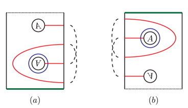
Figure 1. Attaching a $1$- or $2$-handle to the interior of $Y$. (a) Attaching a $1$-handle with both feet on the same boundary component. (b) Attaching a $2$-handle without disconnecting a boundary component. Beyond the dotted lines, each diagram is the same as the standard Heegaard diagram for the identity cobordism.

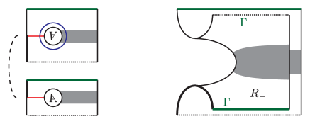
Figure 2. Attaching a $1$-handle to $R_{-}$. Left: part of a bordered-sutured Heegaard diagram corresponding to attaching a $1$-handle to $R_{-}$. Right: an illustration of attaching a $1$-handle to $R_{-}$. The shaded parts of the diagrams on the left and right correspond, as do the thick parts of the left boundary of each.

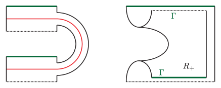
Figure 3. Attaching a $1$-handle to $R_{+}$. Left: part of a bordered-sutured Heegaard diagram corresponding to attaching a $1$-handle to $R_{+}$. Right: the corresponding $1$-handle being attached to $R_{+}$.

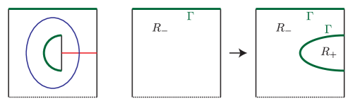
Figure 4. A cup in $R_{-}$, i.e., an $R_{+}$-cup. Left: the Heegaard diagram. Note that this piece of the diagram has two boundary components. Right: the effect on part of $R_{-}$. The rest of $R_{\pm}$ is unchanged. For a cap instead of a cup, rotate the diagram by $\pi$.

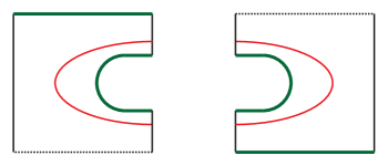
Figure 5. A cup or cap in $R_{+}$, i.e., an $R_{-}$-cup. Left: the Heegaard diagram for a cup. Right: the Heegaard diagram for a cap. The effect of the cup on $R_{\pm}$ is similar to Figure 4, except with the roles of $R_{\pm}$ exchanged.

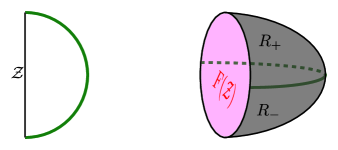
Figure 6. Capping off a pointless bordered arc. Left: the relevant component of the bordered-sutured Heegaard diagram. The bordered boundary is on the left, and thin, and the sutured boundary is on the right, and thick. The rest of the Heegaard diagram is the standard Heegaard diagram fro the identity map of $\mathcal{Z}^{\prime}$. Right: the non-identity component of the corresponding bordered-sutured cobordism. The bordered boundary is lightly shaded and $R_{\pm}$ are darkly shaded.

Our first milestone is to prove that any bordered-sutured manifold can be decomposed into these basic pieces. We start by showing that arcslides generate the mapping class groupoid in the bordered-sutured case. (In the connected boundary case, this is well-known [Pen87, Ben10, LOT14].)

Definition 7.1.

The mapping class groupoid has objects the arc diagrams $\mathcal{Z}$. The morphism set $\operatorname{Hom}(\mathcal{Z}_{1},\mathcal{Z}_{2})$ is the set of isotopy classes of diffeomorphisms $F(\mathcal{Z}_{1})\to F(\mathcal{Z}_{2})$ taking the arcs $S_{+}\subset\partial F(\mathcal{Z}_{1})$ homeomorphically to the arcs $S_{+}\subset F(\mathcal{Z}_{2})$.

The mapping class groupoid is a disjoint union of groupoids, one for each topological type of sutured surface.

Given an arcslide from $\mathcal{Z}_{1}$ to $\mathcal{Z}_{2}$ there is a corresponding arcslide diffeomorphism from $F(\mathcal{Z}_{1})$ to $F(\mathcal{Z}_{2})$ (see, e.g., [LOT14, Figure 3]). Abusing terminology, we will typically refer to the arcslide diffeomorphism as an arcslide.

Lemma 7.2.

The arcslide diffeomorphisms generate the mapping class groupoid.

Proof.

Fix arc diagrams $\mathcal{Z}_{1}$ and $\mathcal{Z}_{2}$ and a diffeomorphism $\phi\nobreak\mskip 2.0mu\mathpunct{}\nonscript\mkern-3.0mu{:}\penalty 300\mskip 6.0mu plus 1.0muF(\mathcal{Z}_{1})\to F(\mathcal{Z}_{2})$ respecting the markings of the boundary. Choose Morse functions $f_{i}$ on $F(\mathcal{Z}_{i})$ compatible with the arc diagrams ($\mathcal{Z}$-compatible Morse functions in Zarev’s language [Zar09, Definition 2.3]), and so that there is a neighborhood $U$ of $S_{+}\subset\partial F(\mathcal{Z}_{2})$ so that $f_{1}|_{\phi^{-1}(U)}=f_{2}\circ\phi|_{\phi^{-1}(U)}$. The functions $f_{1}$ and $f_{2}\circ\phi$ can be connected by a $1$-parameter family of Morse functions $f_{t}$, $t\in[0,1]$, all of which agree with $f_{1}$ over $\phi^{-1}(U)$. (See, e.g., [Sha98].) For a generic choice of metric, there are finitely many $t$ for which $f_{t}$ is not Morse-Smale, because of a flow between two index $1$ critical points. These are the arcslides. ∎

A second lemma allows us to restrict to bordered-sutured manifolds with connected boundary. Given a bordered-sutured manifold $\mathcal{Y}=(Y,\Gamma,\phi)$, a decomposing disk is a disk $D$ in $Y$ with boundary in the sutured boundary of $Y$, and so that $\partial D\cap R_{+}$ and $\partial D\cap R_{-}$ each consists of one arc. Given a decomposing disk $D$, $Y\setminus\mathrm{nbd}(D)$ can be made into a bordered-sutured manifold by including $\partial\mathrm{nbd}(D)$ in the sutured boundary, and adding a single arc in each of the components of $\partial\mathrm{nbd}(D)$ to $\Gamma$. The bordered boundary of $Y\setminus\mathrm{nbd}(D)$ inherits a parametrization from $Y$. We say that such bordered-sutured manifolds differ by a disk decomposition.

Lemma 7.3.

If $\mathcal{Y}$ and $\mathcal{Y}^{\prime}$ are bordered-sutured manifolds which differ by a disk decomposition then $\widehat{\mathit{BSD}}(\mathcal{Y})\simeq\widehat{\mathit{BSD}}(\mathcal{Y}^{\prime})$.

Proof.

This is a special case of Zarev’s surface decomposition theorem [Zar09, Theorem 10.6], but in this case is easy to see directly. Specifically, we can find a bordered-sutured Heegaard diagram $(\Sigma,\boldsymbol{\alpha},\boldsymbol{\beta})$ for $\mathcal{Y}$ so that $D\cap\Sigma$ is a single arc $\eta$ with $\partial\eta$ contained in the sutures of $\Sigma$ and so that $\eta$ is disjoint from $\boldsymbol{\alpha}$ and $\boldsymbol{\beta}$. Then $(\Sigma\setminus\mathrm{nbd}(\eta),\boldsymbol{\alpha},\boldsymbol{\beta})$ is a bordered-sutured Heegaard diagram for $\mathcal{Y}^{\prime}$, where we include $\partial\mathrm{nbd}(\eta)$ as part of the sutured boundary of $\Sigma\setminus\mathrm{nbd}(\eta)$. If we choose corresponding almost complex structures, the generators and differential for $\widehat{\mathit{BSD}}(\Sigma,\boldsymbol{\alpha},\boldsymbol{\beta})$ and $\widehat{\mathit{BSD}}(\Sigma\setminus\mathrm{nbd}(\eta),\boldsymbol{\alpha},\boldsymbol{\beta})$ are exactly the same. ∎

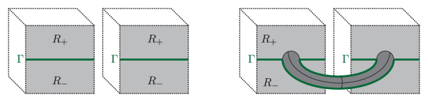
Figure 7. Attaching a 3-dimensional $1$-handle to $\Gamma$. Left: part of a bordered-sutured cobordism $Y$. The part of $\partial Y$ shown is lightly shaded. Outside the dashed cubes, $Y$ is arbitrary. Right: the result of attaching a $1$-handle to connect these two components of $\partial Y$.

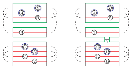
Figure 8. Making the boundary connected. Left: a bordered-sutured Heegaard diagram for a bordered-sutured manifold with two boundary components. Right: a bordered-sutured Heegaard diagram for a bordered-sutured manifold with connected boundary, and an arc $\eta$, so that a disk decomposition along $\eta$ gives the diagram on the left.

In particular, given any bordered-sutured manifold $\mathcal{Y}=(Y,\Gamma,\phi)$ one can attach $3$-dimensional $1$-handles to $\partial Y$ with attaching points on $\Gamma$ to make $\partial Y$ connected, without changing $\widehat{\mathit{BSD}}(\mathcal{Y})$. In this operation, each attaching disk intersects $\Gamma$ in an arc, and $\Gamma$ changes by surgery at the attaching points so that these arcs are replaced with two parallel arcs that go over the $1$-handle and the result is a bordered-sutured manifold. See Figure 7 for an illustration of this operation and Figure 8 for the corresponding operation on Heegaard diagrams.

Thus, it suffices to compute $\widehat{\mathit{BSD}}(\mathcal{Y})$ where $\mathcal{Y}$ has connected boundary.

Lemma 7.4.

Up to disk decomposition, any bordered-sutured manifold $\mathcal{Y}=(Y,\Gamma,\phi\nobreak\mskip 2.0mu\mathpunct{}\nonscript\mkern-3.0mu{:}\penalty 300\mskip 6.0mu plus 1.0muF(\mathcal{Z})\to\partial Y)$ can be decomposed as a union of the seven basic bordered-sutured pieces above.

Proof.

Since attaching a $1$-handle to $\Gamma$ is the inverse of a disk decomposition, we may assume that $\partial Y$ is connected and that the sutured part of $\partial Y$ is connected.

Choose some parametrization $\psi\nobreak\mskip 2.0mu\mathpunct{}\nonscript\mkern-3.0mu{:}\penalty 300\mskip 6.0mu plus 1.0muF(\mathcal{Z}^{\prime})\to\partial Y$ of $\partial Y$ by the surface associated to a pointed matched circle $\mathcal{Z}^{\prime}$. Then we can view $\mathcal{Y}$ as the composition of the bordered manifold $(Y,\psi)$ and a bordered-sutured cobordism $(Y^{\prime},\Gamma^{\prime})$ from $F(\mathcal{Z}^{\prime})$ to $F(\mathcal{Z})$ so that $Y^{\prime}$ is topologically a cylinder $[0,1]\times F(\mathcal{Z}^{\prime})$.

From the bordered case [LOT14, Section 8], we can decompose $(Y,\psi)$ as a composition of arcslides and $1$- and $2$-handle attachments to the bordered boundary. It remains to decompose $Y^{\prime}$ into $1$- and $2$-handle attachments to $R_{\pm}$, $R_{\pm}$ cups and caps, capping pointless arcs, and arcslides. To this end, let $\partial_{s}Y^{\prime}\subset\partial Y^{\prime}$ denote the sutured boundary. Choose a Morse function $f\nobreak\mskip 2.0mu\mathpunct{}\nonscript\mkern-3.0mu{:}\penalty 300\mskip 6.0mu plus 1.0mu\partial_{s}Y^{\prime}\to[0,1]$ so that $f^{-1}(0)=\partial_{s}Y^{\prime}\cap F(\mathcal{Z}^{\prime})$, $f^{-1}(1)=\partial_{s}Y^{\prime}\cap F(\mathcal{Z})$, $f$ has no index $0$ critical points, and each critical level of $f$ has a single critical point. By a possibly large perturbation of the sutures, we can arrange that for each $t\in[0,1]$ and each connected component $C$ of $f^{-1}(t)$, $C\cap\Gamma\neq\emptyset$. Further perturbing the sutures slightly, we may assume that:

1. If $p_{1},\dots,p_{k}$ are the critical points of $f$ then each $p_{i}$ is in the interior of either $R_{+}$ or $R_{-}$ (i.e., $p_{i}\not\in\Gamma$).

2. The restriction of $f$ to $\Gamma$ is a Morse function, with critical points $q_{1},\dots,q_{\ell}$, say.

3. The real numbers $f(p_{1}),\dots,f(p_{k}),f(q_{1}),\dots,f(q_{\ell})$ are all distinct.

Choose $0=t_{0}<t_{1}<\dots<t_{k+\ell}=1$ so that each $f^{-1}((t_{i},t_{i+1}))$ contains exactly one $p_{i}$ or $q_{i}$. Then $f^{-1}([t_{i},t_{i+1}])$ corresponds to a $1$-handle attachment to $R_{+}$ or $R_{-}$ (for a $p_{i}$) or a $R_{+}$- or $R_{-}$-cup or cap or capping off a pointless bordered arc (for a $q_{i}$). Let

$$\mathcal{Y}_{i}=(Y_{i},\ \phi_{i,L}\nobreak\mskip 2.0mu\mathpunct{}\nonscript\mkern-3.0mu{:}\penalty 300\mskip 6.0mu plus 1.0mu-F(\mathcal{Z}_{i,L})\to\partial_{L}Y_{i},\ \phi_{i,R}\nobreak\mskip 2.0mu\mathpunct{}\nonscript\mkern-3.0mu{:}\penalty 300\mskip 6.0mu plus 1.0muF(\mathcal{Z}_{i,R})\to\partial_{R}Y_{i})$$

be the corresponding bordered-sutured cobordism (parametrized as in Figures 2–6, above). So, in particular, $Y_{i}=[0,1]\times(f^{-1}([t_{i},1])\cup F(\mathcal{Z}))$. For $i=1,\dots,k+\ell-2$, let $\mathcal{Y}_{i,i+1}$ be the mapping cylinder of a composition of arclides from $\phi_{i,R}$ to $\phi_{i+1,L}$. Let $\mathcal{Y}_{k+\ell-1,k+\ell}$ be the mapping cylinder of a sequence of arcslides from $\phi_{k+\ell}$ to $\phi$. Then,

$$\mathcal{Y}=(Y,\psi)\cup\mathcal{Y}_{1}\cup\mathcal{Y}_{1,2}\cup\mathcal{Y}_{2}\cup\cdots\cup\mathcal{Y}_{k+\ell-1,k+\ell}\cup\mathcal{Y}_{k+\ell-1}\cup\mathcal{Y}_{k+\ell-1,k+\ell},$$

as bordered-sutured manifolds. This completes the proof. ∎

Our next task is to compute the bordered-sutured modules associated to the seven basic bordered-sutured pieces. We start with some tools for deducing bordered-sutured computations from bordered computations.

Definition 7.5.

Let $\mathcal{Z}=(Z,\mathbf{a},M)$ and $\mathcal{Z}^{\prime}=(Z^{\prime},\mathbf{a}^{\prime},M^{\prime})$ be arc diagrams. We say that $\mathcal{Z}$ is a subdiagram of $\mathcal{Z}^{\prime}$ if there is an embedding $\phi\nobreak\mskip 2.0mu\mathpunct{}\nonscript\mkern-3.0mu{:}\penalty 300\mskip 6.0mu plus 1.0muZ\to Z^{\prime}$ so that $\phi(\mathbf{a})\subset\mathbf{a}^{\prime}$ and $M$ is induced from $M^{\prime}$. Note that we do not require that $\phi$ be proper, i.e., send the boundary of $Z$ to the boundary of $Z^{\prime}$, or that $\phi^{-1}(\mathbf{a}^{\prime})=\mathbf{a}$. If $\phi(\mathbf{a})=\mathbf{a}^{\prime}$ (so, in particular, $\phi^{-1}(\mathbf{a}^{\prime})=\mathbf{a}$) then we say that $\mathcal{Z}$ is a full subdiagram of $\mathcal{Z}^{\prime}$.

Similarly, let $\mathcal{H}=(\Sigma,\boldsymbol{\alpha},\boldsymbol{\beta},\mathbf{z})$ and $\mathcal{H}^{\prime}=(\Sigma^{\prime},\boldsymbol{\alpha}^{\prime},\boldsymbol{\beta}^{\prime},\mathbf{z}^{\prime})$ be bordered-sutured Heegaard diagrams. We say that $\mathcal{H}$ is a subdiagram of $\mathcal{H}^{\prime}$ if there is an embedding $\phi\nobreak\mskip 2.0mu\mathpunct{}\nonscript\mkern-3.0mu{:}\penalty 300\mskip 6.0mu plus 1.0mu\Sigma\to\Sigma^{\prime}$ with the following properties:

1. $\phi$ sends the bordered boundary of $\Sigma$ to the bordered boundary of $\Sigma^{\prime}$.

2. $\phi(\boldsymbol{\alpha})\subset\boldsymbol{\alpha}^{\prime}$.

3. $\phi(\boldsymbol{\beta})=\boldsymbol{\beta}^{\prime}$ and $\phi(\boldsymbol{\alpha})$ contains every circle in $\boldsymbol{\alpha}^{\prime}$.

If further $\phi(\boldsymbol{\alpha})=\boldsymbol{\alpha}^{\prime}$ and then we say that $\mathcal{H}$ is a full subdiagram of $\mathcal{H}^{\prime}$.

In other words, a full subdiagram is obtained by turning some of the bordered boundary of $\Sigma$ into sutured boundary $\mathbf{z}$, and in a non-full subdiagram one can also forget some $\alpha$-arcs. See Figure 9 for some examples of subdiagrams.

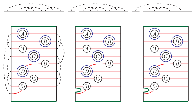
Figure 9. Examples of subdiagrams of arc diagrams and Heegaard diagrams. Top: a pointed matched circle $\mathcal{Z}$, a full subdiagram of $\mathcal{Z}$, and a non-full subdiagram of $\mathcal{Z}$. Bottom: the standard Heegaard diagram for an arcslide, a full subdiagram of this Heegaard diagram, and a non-full subdiagram of this Heegaard diagram.

If $\mathcal{Z}$ is a subdiagram of $\mathcal{Z}^{\prime}$ then there is an injective homomorphism $i\nobreak\mskip 2.0mu\mathpunct{}\nonscript\mkern-3.0mu{:}\penalty 300\mskip 6.0mu plus 1.0mu\mathcal{A}(\mathcal{Z})\to\mathcal{A}(\mathcal{Z}^{\prime})$ obtained by regarding a strand diagram in $\mathcal{Z}$ as lying in $\mathcal{Z}^{\prime}$. If $\mathcal{Z}$ is a full subdiagram of $\mathcal{Z}^{\prime}$ then there is also a projection map $p\nobreak\mskip 2.0mu\mathpunct{}\nonscript\mkern-3.0mu{:}\penalty 300\mskip 6.0mu plus 1.0mu\mathcal{A}(\mathcal{Z}^{\prime})\to\mathcal{A}(\mathcal{Z})$ which is the identity on strand diagrams contained entirely in $\mathcal{Z}$ and sends any strand diagram not entirely contained in $\mathcal{Z}$ to $0$. Associated to $i$ is a restriction of scalars functor

$$i^{*}\nobreak\mskip 2.0mu\mathpunct{}\nonscript\mkern-3.0mu{:}\penalty 300\mskip 6.0mu plus 1.0mu\mathsf{Mod}_{\mathcal{A}(\mathcal{Z}^{\prime})}\to\mathsf{Mod}_{\mathcal{A}(\mathcal{Z})}$$

and associated to $p$ is an extension of scalars functor

$$p_{*}\nobreak\mskip 2.0mu\mathpunct{}\nonscript\mkern-3.0mu{:}\penalty 300\mskip 6.0mu plus 1.0mu{}^{\mathcal{A}(\mathcal{Z}^{\prime})}\mskip-1.80002mu\mathsf{Mod} \to{}^{\mathcal{A}(\mathcal{Z})}\mskip-1.80002mu\mathsf{Mod}$$

$${}^{\mathcal{A}(\mathcal{Z}^{\prime})}\mskip-1.80002muP \mapsto{}^{\mathcal{A}(\mathcal{Z})}\mskip-1.80002mu[p]_{\mathcal{A}(\mathcal{Z}^{\prime})}\boxtimes{}^{\mathcal{A}(\mathcal{Z}^{\prime})}\mskip-1.80002muP,$$

where ${}^{\mathcal{A}(\mathcal{Z})}\mskip-1.80002mu[p]_{\mathcal{A}(\mathcal{Z}^{\prime})}$ denotes the rank $1$ type $\mathit{DA}$ bimodule associated to $p$ [LOT15, Definition 2.2.48].

Lemma 7.6.

If $\mathcal{H}$ is a subdiagram of $\mathcal{H}^{\prime}$ then $\widehat{\mathit{BSA}}(\mathcal{H})\cong i^{*}\widehat{\mathit{BSA}}(\mathcal{H}^{\prime})$. If $\mathcal{H}$ is a full subdiagram of $\mathcal{H}^{\prime}$ then $\widehat{\mathit{BSD}}(\mathcal{H})\cong p_{*}\widehat{\mathit{BSD}}(\mathcal{H}^{\prime})$.

(Compare [LOT15, Sections 6.1 and 6.2].)

Proof.

This is immediate from the definitions. ∎

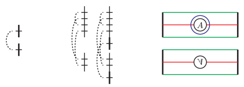
Figure 10. The diagram $\mathcal{Z}_{b}$ and its use. Left: the arc diagram $\mathcal{Z}_{b}$. Center: an arc diagram which is not a full subdiagram of a pointed matched circle and the result of gluing this diagram to $\mathcal{Z}_{b}$, to give an arc diagram which is a full subdiagram of a pointed matched circle. Right: the standard Heegaard diagram for the identity cobordism of $\mathcal{Z}_{b}$.

Let $\mathcal{Z}_{b}$ be the arc diagram with two intervals so that $\mathbf{a}$ has a single point on each. See Figure 10.

Lemma 7.7.

Let $\mathcal{Z}$ be an arc diagram. Then there is a pointed matched circle $\overline{\mathcal{Z}}$ so that either $\mathcal{Z}$ or $\mathcal{Z}\amalg\mathcal{Z}_{b}$ is a full subdiagram of $\overline{\mathcal{Z}}$.

Proof.

Write $\mathcal{Z}=(Z,\mathbf{a},M)$. There is a pairing of the endpoints of $Z$ by saying that $z$ is paired with $z^{\prime}$ if, after doing surgery on $Z$ according to $(\mathbf{a},M)$ the points $z$ and $z^{\prime}$ are on the same connected component. If $Z$ has more than two components then we can choose a top endpoint $z$ of an interval $I$ and a bottom endpoint $z^{\prime}$ of a different interval $I^{\prime}$ so that $z$ is not paired to $z^{\prime}$ and glue $z$ to $z^{\prime}$. If $Z$ has two components then either we can choose such a pair of points or we can do so after gluing on a copy of $\mathcal{Z}_{b}$ as in Figure 10. This gluing gives an arc diagram with one fewer intervals. ∎

Lemma 7.8.

If $\mathcal{H}=\mathcal{H}_{1}\amalg\mathcal{H}_{2}$ is a disconnected bordered-sutured Heegaard diagram then

$$\widehat{\mathit{BSD}}(\mathcal{H})\cong\widehat{\mathit{BSD}}(\mathcal{H}_{1})\otimes_{\mathbb{F}_{2}}\widehat{\mathit{BSD}}(\mathcal{H}_{2}).$$

Proof.

This is immediate from the definitions. ∎

There is another operation which has essentially no effect on the bordered-sutured invariants. Suppose that $\mathcal{H}$ is a bordered-sutured Heegaard diagram and $\eta$ is an arc in $\mathcal{H}$ starting on the sutured boundary of $\mathcal{H}$ and ending on the bordered boundary, and so that $\eta$ is disjoint from the $\alpha$- and $\beta$-curves. Cutting along $\eta$ gives a new bordered-sutured Heegaard diagram $\mathcal{H}^{\prime}$. We will say that $\mathcal{H}^{\prime}$ is obtained from $\mathcal{H}$ by a safe cut. The modules $\widehat{\mathit{BSD}}(\mathcal{H})$ and $\widehat{\mathit{BSD}}(\mathcal{H}^{\prime})$ are essentially the same, the subtlety being that they are over different algebras.

Lemma 7.9.

Suppose that $\mathcal{H}^{\prime}$ is obtained from $\mathcal{H}$ by a safe cut. Let $\mathcal{Z}$ (respectively $\mathcal{Z}^{\prime}$) be the arc diagram on the boundary of $\mathcal{H}$ (respectively $\mathcal{H}^{\prime}$). Then there is an inclusion $i\nobreak\mskip 2.0mu\mathpunct{}\nonscript\mkern-3.0mu{:}\penalty 300\mskip 6.0mu plus 1.0mu\mathcal{A}(\mathcal{Z}^{\prime})\hookrightarrow\mathcal{A}(\mathcal{Z})$ (induced by the inclusion of $\mathcal{Z}^{\prime}$ into $\mathcal{Z}$) and a projection $p\nobreak\mskip 2.0mu\mathpunct{}\nonscript\mkern-3.0mu{:}\penalty 300\mskip 6.0mu plus 1.0mu\mathcal{A}(\mathcal{Z})\to\mathcal{A}(\mathcal{Z}^{\prime})$ (induced by setting any strand diagram not contained in $\mathcal{Z}^{\prime}$ to zero) so that

(7.10) $$\widehat{\mathit{BSD}}(\mathcal{H}) \simeq i_{*}\widehat{\mathit{BSD}}(\mathcal{H}^{\prime})$$

(7.11) $$\widehat{\mathit{BSD}}(\mathcal{H}^{\prime}) \simeq p_{*}\widehat{\mathit{BSD}}(\mathcal{H})$$

(7.12) $$\widehat{\mathit{BSA}}(\mathcal{H}) \simeq p^{*}\widehat{\mathit{BSA}}(\mathcal{H}^{\prime})$$

(7.13) $$\widehat{\mathit{BSA}}(\mathcal{H}^{\prime}) \simeq i^{*}\widehat{\mathit{BSA}}(\mathcal{H}).$$

(Here, $i_{*}$ and $p_{*}$ are induction, or extension of scalars and $i^{*}$ and $p^{*}$ are restriction of scalars.)

Proof.

Write $\mathcal{H}=(\Sigma,\boldsymbol{\alpha},\boldsymbol{\beta},\mathbf{z})$ and $\mathcal{H}^{\prime}=(\Sigma^{\prime},\boldsymbol{\alpha}^{\prime},\boldsymbol{\beta}^{\prime},\mathbf{z}^{\prime})$. There is a map $\iota\nobreak\mskip 2.0mu\mathpunct{}\nonscript\mkern-3.0mu{:}\penalty 300\mskip 6.0mu plus 1.0mu\Sigma^{\prime}\to\Sigma$ (which is $2$-to-$1$ on the new sutured part of the boundary of $\Sigma^{\prime}$ and $1$-to-$1$ otherwise). Abusing notation, we will also let $\iota$ denote the induced map $\Sigma^{\prime}\times[0,1]\times\mathbb{R}\to\Sigma\times[0,1]\times\mathbb{R}$.

The map $\iota$ induces a bijection of generators, $\mathbf{x}^{\prime}=\{x^{\prime}_{i}\}\mapsto\iota(\mathbf{x}^{\prime})=\{\iota(x^{\prime}_{i})\}$, and a bijection of domains $\iota_{*}\nobreak\mskip 2.0mu\mathpunct{}\nonscript\mkern-3.0mu{:}\penalty 300\mskip 6.0mu plus 1.0mu\pi_{2}(\mathbf{x}^{\prime},\mathbf{y}^{\prime})\to\pi_{2}(\iota(\mathbf{x}^{\prime}),\iota(\mathbf{y}^{\prime}))$. Choose a sufficiently generic almost complex structure $J$ on $\Sigma\times[0,1]\times\mathbb{R}$ [LOT08, Definition 5.7] and let $J^{\prime}=\iota^{*}J$ be the induced almost complex structure on $\Sigma^{\prime}\times[0,1]\times\mathbb{R}$. Then for $B^{\prime}\in\pi_{2}(\mathbf{x}^{\prime},\mathbf{y}^{\prime})$, a map $u\nobreak\mskip 2.0mu\mathpunct{}\nonscript\mkern-3.0mu{:}\penalty 300\mskip 6.0mu plus 1.0muS\to\Sigma^{\prime}\times[0,1]\times\mathbb{R}$ is a $J^{\prime}$-holomorphic curve in the moduli space $\mathcal{M}^{B^{\prime}}(\mathbf{x}^{\prime},\mathbf{y}^{\prime})$ if and only if $\iota\circ u$ is a $J$-holomorphic curve in $\mathcal{M}^{\iota_{*}(B^{\prime})}(\iota(\mathbf{x}^{\prime}),\iota(\mathbf{y}^{\prime}))$. The assignment $u\mapsto\iota\circ u$ is clearly injective; from positivity of domains [LOT08, Proof of Lemma 5.4], it is also surjective.

Thus, if $a\otimes\mathbf{y}$ is a term in $\delta^{1}(\mathbf{x})$ for some generators $\mathbf{x},\mathbf{y}\in\widehat{\mathit{BSD}}(\mathcal{H})$ and strand diagram $a\in\mathcal{A}(\mathcal{Z})$ then $a$ is the image of a strand diagram $a^{\prime}\in\mathcal{A}(\mathcal{Z}^{\prime})$. Further, $a^{\prime}\otimes y^{\prime}$ occurs in the differential of $\mathbf{x}^{\prime}$, where $\iota(\mathbf{x}^{\prime})=\mathbf{x}$ and $\iota(\mathbf{y}^{\prime})=\mathbf{y}$. The results about $\widehat{\mathit{BSD}}$ follow. The proofs for $\widehat{\mathit{BSA}}$ are only notationally different.

(Note that Equation (7.11) is also a special case of Lemmas 7.6 and 7.8.) ∎

Lemma 7.14.

The module $\widehat{\mathit{BSD}}(\mathit{Id}_{\mathcal{Z}_{b}})$ associated to the identity cobordism of $\mathcal{Z}_{b}$ has two generators and trivial differential.

Proof.

Again, this is immediate from the definitions. (See also Figure 10.) ∎

7.1.1. The identity cobordism

Fix an arc diagram $\mathcal{Z}=(Z,\mathbf{a},M)$. Given a set of matched pairs $\mathbf{s}$ in $\mathcal{Z}$, let $\mathbf{s}^{c}$ denote the complementary set of matched pairs, but viewed as lying in $-\mathcal{Z}$. We call the pair of idempotents $I(\mathbf{s})\otimes I(\mathbf{s}^{c})\in\mathcal{A}(\mathcal{Z})\otimes\mathcal{A}(-\mathcal{Z})$ complementary.

A chord in $\mathcal{Z}$ is an interval in $Z$ with endpoints in $\mathbf{a}$. Given a chord $\rho$ in $\mathcal{Z}$ there is a corresponding algebra element $a(\rho)$, which is the sum of all strand diagrams in which $\rho$ is the only moving strand. There is also a corresponding chord $\rho^{\prime}$ in $-\mathcal{Z}$.

Lemma 7.15.

For any arc diagram $\mathcal{Z}$, the bordered-sutured bimodules $\widehat{\mathit{BSDD}}(\mathit{Id}_{\mathcal{Z}})$ associated to the identity cobordism of $\mathcal{Z}$ is generated by the set of pairs of complementary idempotents $(I\otimes J)\in\mathcal{A}(\mathcal{Z})\otimes\mathcal{A}(-\mathcal{Z})$, and has differential

$$\delta^{1}(I\otimes J)=\sum_{I^{\prime}\otimes J^{\prime}}\sum_{\text{chords }\rho}(I\otimes J)(a(\rho)\otimes a(\rho^{\prime}))\otimes(I^{\prime}\otimes J^{\prime}).$$

(Here, the first sum is over the pairs of complementary idempotents.)

Proof.

We deduce this from the corresponding statement for pointed matched circles [LOT14, Theorem 1]. Provisionally, let $\mathit{DDId}(\mathcal{Z})$ be the type $\mathit{DD}$ bimodule described in the statement of the lemma, and let $\widehat{\mathit{BSDD}}(\mathit{Id}_{\mathcal{Z}})$ be the type $\mathit{DD}$ bimodule associated to the standard Heegaard diagram for the identity cobordism of $\mathcal{Z}$ (with respect to any sufficiently generic almost complex structure). We want to show that $\mathit{DDId}(\mathcal{Z})\simeq\widehat{\mathit{BSDD}}(\mathit{Id}_{\mathcal{Z}})$. Note that there is a unique isomorphism of underlying $\mathcal{I}(\mathcal{Z})\otimes\mathcal{I}(-\mathcal{Z})$-modules between $\mathit{DDId}(\mathcal{Z})$ and $\widehat{\mathit{BSDD}}(\mathit{Id}_{\mathcal{Z}})$; we will show that this identification intertwines the operations $\delta^{1}$.

By definition, $\mathit{DDId}(\mathcal{Z}\amalg\mathcal{Z}_{b})\cong\mathit{DDId}(\mathcal{Z})\otimes_{\mathbb{F}_{2}}\mathit{DDId}(\mathcal{Z}_{b})$. Similarly, by Lemma 7.8, $\widehat{\mathit{BSDD}}(\mathit{Id}_{\mathcal{Z}\amalg\mathcal{Z}_{b}})\cong\widehat{\mathit{BSDD}}(\mathit{Id}_{\mathcal{Z}})\otimes_{\mathbb{F}_{2}}\widehat{\mathit{BSDD}}(\mathit{Id}_{\mathcal{Z}_{b}})$. If the unique isomorphism of underlying modules $\mathit{DDId}(\mathcal{Z}\amalg\mathcal{Z}_{b})\cong\widehat{\mathit{BSDD}}(\mathit{Id}_{\mathcal{Z}\amalg\mathcal{Z}_{b}})$ intertwines the operations $\delta^{1}$ then so does the unique isomorphism $\mathit{DDId}(\mathcal{Z})\cong\widehat{\mathit{BSDD}}(\mathit{Id}_{\mathcal{Z}})$. So, by Lemma 7.7, we may assume that $\mathcal{Z}$ is a full subdiagram of a pointed matched circle $\overline{\mathcal{Z}}$. By Lemma 7.6, $\widehat{\mathit{BSDD}}(\mathit{Id}_{\mathcal{Z}})\cong p_{*}\widehat{\mathit{BSDD}}(\mathit{Id}_{\overline{\mathcal{Z}}})$. Further, by inspection, $\mathit{DDId}(\mathcal{Z})\cong p_{*}\mathit{DDId}(\overline{\mathcal{Z}})$. Finally, from the bordered case [LOT14, Theorem 1], $\widehat{\mathit{BSDD}}(\mathit{Id}_{\overline{\mathcal{Z}}})\cong\mathit{DDId}(\overline{\mathcal{Z}})$. The result follows. ∎

We note that we have also computed $\widehat{\mathit{BSAA}}(\mathit{Id}_{\mathcal{Z}})$, by an analogue of a duality result in the bordered case [LOT11, Theorem 5]:

Proposition 7.16.

For any arc diagram $\mathcal{Z}$ there is a homotopy equivalence of $A_{\infty}$-bimodules

$$\widehat{\mathit{BSAA}}(\mathit{Id}_{\mathcal{Z}})_{\mathcal{A}(\mathcal{Z}),\mathcal{A}(-\mathcal{Z})}\\ \simeq\operatorname{Mor}_{\mathcal{A}(\mathcal{Z})}\bigl{(}(\mathcal{A}(-\mathcal{Z})\otimes_{\mathbb{F}_{2}}\mathcal{A}(\mathcal{Z}))_{\mathcal{A}(-\mathcal{Z})\otimes\mathcal{A}(\mathcal{Z})}\boxtimes{}^{\mathcal{A}(-\mathcal{Z})\otimes\mathcal{A}(\mathcal{Z})}\mskip-1.80002mu\widehat{\mathit{BSDD}}(\mathit{Id}_{\mathcal{Z}}),\ \mathcal{A}(\mathcal{Z})\bigr{)}$$

Proof.

The proof is the same as in the bordered case [LOT11, Theorem 5]. ∎

Corollary 7.17.

If $\mathcal{Y}$ is a bordered-sutured cobordism from $\mathcal{Z}_{1}$ to $\mathcal{Z}_{2}$ then

$${}^{\mathcal{A}(\mathcal{Z}_{1})}\mskip-1.80002mu\widehat{\mathit{BSDA}}(\mathcal{Y})_{\mathcal{A}(\mathcal{Z}_{2})}\simeq\operatorname{Mor}^{\mathcal{A}(-\mathcal{Z}_{2})}\bigl{(}\mathcal{A}(\mathcal{Z}_{2})\boxtimes\widehat{\mathit{BSDD}}(\mathit{Id}_{\mathcal{Z}_{2}}),{}^{\mathcal{A}(\mathcal{Z}_{1}),\mathcal{A}(-\mathcal{Z}_{2})}\mskip-1.80002mu\widehat{\mathit{BSDD}}(\mathcal{Y})\bigr{)}.$$

(Here, $\operatorname{Mor}$ is the chain complex of type $D$ structure morphisms.)

Proof.

This is immediate from Proposition 7.16 and the fact that $\mathcal{A}(-\mathcal{Z}_{2})\boxtimes\cdot$ is a quasi-equivalence of dg categories from the category of type $D$ structures to the category of $A_{\infty}$-modules. ∎

7.1.2. Arcslides

Let $\phi\nobreak\mskip 2.0mu\mathpunct{}\nonscript\mkern-3.0mu{:}\penalty 300\mskip 6.0mu plus 1.0mu\mathcal{Z}\to\mathcal{Z}^{\prime}$ be an arcslide and $\mathcal{H}_{\phi}$ the standard Heegaard diagram for $\phi$ [LOT14, Figure 16] (see also Figures 9 and 11). Let $\overline{\mathcal{Z}}$ be the pointed matched circle from Lemma 7.7 and $\overline{\phi}\nobreak\mskip 2.0mu\mathpunct{}\nonscript\mkern-3.0mu{:}\penalty 300\mskip 6.0mu plus 1.0mu\overline{\mathcal{Z}}\to\overline{\mathcal{Z}}^{\prime}$ the corresponding arcslide.

Proposition 7.18.

The bimodule $\widehat{\mathit{BSDD}}(\mathcal{H}_{\phi})$ is generated by the near-complementary pairs of idempotents [LOT14, Definition 1.5] in $\mathcal{A}(\mathcal{Z})\otimes\mathcal{A}(\mathcal{Z}^{\prime})$ and the differential is given by

$$\delta^{1}(I\otimes J)=\sum_{I^{\prime}\otimes J^{\prime}}(I\otimes J)A\otimes(I^{\prime}\otimes J^{\prime})$$

where $A$ is the sum of all near-chords in $(\overline{\mathcal{Z}},\overline{\mathcal{Z}}^{\prime})$ [LOT14, Definition 4.19] which are contained in $(\mathcal{Z},\mathcal{Z}^{\prime})$ if $\overline{\phi}$ is an underslide, and is the sum of all near-chords in $(\overline{\mathcal{Z}},\overline{\mathcal{Z}}^{\prime})$ determined by any basic choice [LOT14, Definition 4.32] which are contained in $(\mathcal{Z},\mathcal{Z}^{\prime})$ if $\overline{\phi}$ is an overslide.

Proof.

The proof is similar to the proof of Proposition 7.15. By Lemmas 7.8 and 7.14, it suffices to consider the case that $\mathcal{Z}$ (rather than $\mathcal{Z}\amalg\mathcal{Z}_{b}$) is a full subdiagram of a pointed matched circle. In this case, $\mathcal{H}_{\phi}$ is a full subdiagram of the standard Heegaard diagram for $\overline{\phi}$. So, this is immediate from Lemma 7.6 and the computation for pointed matched circles [LOT14, Propositions 4.20 and 4.37]. ∎

7.1.3. Interior 1- and 2-handle attachments

In this section we will give the bimodule for a $2$-handle attachment; the bimodule for a $1$-handle attachment is the same except for exchanging which action corresponds to which boundary component.

Before giving the bimodule we need a little notation for the algebra $\mathcal{A}(T^{2})$ associated to the torus (with two boundary sutures). This algebra is the path algebra with relations

$$\vbox{\hbox{$\leavevmode\hbox to69.91pt{\vbox to47.6pt{\text{[drawing]}}}$}}/(\rho_{2}\rho_{1}=\rho_{3}\rho_{2}=0). \iota_{0} \iota_{1} \rho_{1} \rho_{2} \rho_{3} \iota_{0} \iota_{1} \rho_{1} \rho_{2} \rho_{3}$$

(Compare [LOT08, Section 11.1]. We are following the convention that $\rho_{1}\rho_{2}$ means the arrow labeled $\rho_{1}$ followed by the arrow labeled $\rho_{2}$; this is the opposite of composition order. So, for instance, $\rho_{1}=\iota_{0}\rho_{1}\iota_{1}$.)

Let $H_{\infty}$ be the $\infty$-framed solid torus, with boundary the genus $1$ pointed matched circle. The type $D$ structure $\widehat{\mathit{CFD}}(H_{\infty})$ over $\mathcal{A}(T^{2})$ has a single generator $r$, and differential

$$\delta^{1}(r)=(\rho_{2}\rho_{3})\otimes r.$$

[LOT15, Section 11.2]. We can regard $\widehat{\mathit{CFD}}(H_{\infty})$ as a type $\mathit{DD}$ bimodule over $\mathcal{A}(T^{2})$ and $\mathbb{F}_{2}$.

Given an arc diagram $\mathcal{Z}$, let $\mathit{Id}_{\mathcal{Z}}$ denote the identity cobordism of $F(\mathcal{Z})$, and $\widehat{\mathit{BSDD}}(\mathit{Id}_{\mathcal{Z}})$ the corresponding type $\mathit{DD}$ bimodule.

Consider a (non-disconnecting) $2$-handle attachment as in Figure 1(b) where the pointed matched circle on the right is $\mathcal{Z}_{R}$ and the pointed matched circle on the left is $\mathcal{Z}_{L}$. Then there is an inclusion map

(7.19) $$\mathcal{A}(T^{2})\otimes_{\mathbb{F}_{2}}\mathcal{A}(\mathcal{Z}_{R})\hookrightarrow\mathcal{A}(\mathcal{Z}_{L}).$$

Proposition 7.20.

The type $\mathit{DD}$ bimodule for a $2$-handle attachment from $\mathcal{A}(\mathcal{Z}_{L})$ to $\mathcal{A}(\mathcal{Z}_{R})$ is the image of $\widehat{\mathit{BSDD}}(\mathit{Id}_{\mathcal{Z}_{R}})\otimes_{\mathbb{F}_{2}}\widehat{\mathit{CFD}}(H_{\infty})$ under extension of scalars with respect to the map (7.19).

Proof.

This is immediate from Lemmas 7.9 and 7.8. ∎

7.1.4. Attaching handles to $R_{\pm}$

We describe the bimodules for attaching a $1$-handle to $R_{-}$ or $R_{+}$.

Let $\mathcal{Z}^{\prime}=(Z^{\prime},\mathbf{a}^{\prime},M^{\prime})$ be an arc diagram, and let $z_{1},z_{2}$ be terminal endpoints of two different components of $Z^{\prime}$. Let $\mathcal{Z}=(Z^{\prime},\mathbf{a},M)$ where $\mathbf{a}=\mathbf{a}^{\prime}\cup\{b,c\}$ and $b$ is slightly below $z_{1}$ and $c$ is slightly below $z_{2}$; and $M$ agrees with $M^{\prime}$ on $\mathbf{a}^{\prime}$ and pairs $b$ and $c$. That is, $-\mathcal{Z}$ (respectively $\mathcal{Z}^{\prime}$) is as on the left (respectively right) of Figure 2. Given a strand diagram $a\in\mathcal{A}(\mathcal{Z}^{\prime})$, composing $a$ with the inclusion map $i\nobreak\mskip 2.0mu\mathpunct{}\nonscript\mkern-3.0mu{:}\penalty 300\mskip 6.0mu plus 1.0mu\mathcal{Z}^{\prime}\hookrightarrow\mathcal{Z}$ gives a strand diagram $i(a)\in\mathcal{A}(\mathcal{Z})$, and this induces an algebra homomorphism $i_{\ooalign{\scriptsize$\mathrm{bc}$\cr\rule[0.90417pt]{6.02777pt}{1.0pt}}}\nobreak\mskip 2.0mu\mathpunct{}\nonscript\mkern-3.0mu{:}\penalty 300\mskip 6.0mu plus 1.0mu\mathcal{A}(\mathcal{Z}^{\prime})\hookrightarrow\mathcal{A}(\mathcal{Z})$. There is an induced homomorphism

$$(i_{\ooalign{\scriptsize$\mathrm{bc}$\cr\rule[0.90417pt]{6.02777pt}{1.0pt}}}\otimes\mathit{Id})\nobreak\mskip 2.0mu\mathpunct{}\nonscript\mkern-3.0mu{:}\penalty 300\mskip 6.0mu plus 1.0mu\mathcal{A}(\mathcal{Z}^{\prime})\otimes\mathcal{A}(-\mathcal{Z}^{\prime})\hookrightarrow\mathcal{A}(\mathcal{Z})\otimes\mathcal{A}(-\mathcal{Z}^{\prime}).$$

Proposition 7.21.

If $\mathcal{Y}$ is the bordered-sutured cobordism from $\mathcal{A}(\mathcal{Z})$ to $\mathcal{A}(\mathcal{Z}^{\prime})$ associated to a $1$-handle attachment to $R_{-}$ (Figure 2) then there is a homotopy equivalence

$${}^{\mathcal{A}(\mathcal{Z}),\mathcal{A}(-\mathcal{Z}^{\prime})}\mskip-1.80002mu\widehat{\mathit{BSDD}}(\mathcal{Y})\simeq(i_{\ooalign{\scriptsize$\mathrm{bc}$\cr\rule[0.90417pt]{6.02777pt}{1.0pt}}}\otimes\mathit{Id})_{*}{}^{\mathcal{A}(\mathcal{Z}^{\prime}),\mathcal{A}(-\mathcal{Z}^{\prime})}\mskip-1.80002mu\widehat{\mathit{BSDD}}(\mathit{Id}_{\mathcal{Z}^{\prime}}).$$

Proof.

This is immediate from Lemma 7.9 and the observation that there are no holomorphic curves with image in the non-identity part of the Heegaard diagram from Figure 2. ∎

Next, let $\mathcal{Z}=(Z,\mathbf{a},M)$ be an arc diagram. Suppose that $b$ and $c$ are points in $\mathbf{a}$ which are adjacent to terminal endpoints of arcs in $Z$ and so that $b$ is matched with $c$. Let $\mathcal{Z}^{\prime}=(Z^{\prime},\mathbf{a}^{\prime},M^{\prime})$ be the result of performing surgery on the pair $(b,c)$, with $\mathbf{a}^{\prime}=\mathbf{a}\setminus\{b,c\}$. So, $-\mathcal{Z}$ (respectively $\mathcal{Z}^{\prime}$) is the arc diagram on the left (respectively right) of Figure 3.

There is an inclusion map $i_{\mathrm{bc}}\nobreak\mskip 2.0mu\mathpunct{}\nonscript\mkern-3.0mu{:}\penalty 300\mskip 6.0mu plus 1.0mu\mathcal{A}(\mathcal{Z}^{\prime})\hookrightarrow\mathcal{A}(\mathcal{Z})$, defined as follows. Recall that a strand diagram in $\mathcal{Z}$ consists of subsets $S$, $T$ of the set of matched pairs in $\mathbf{a}$ and a collection of arcs with initial endpoints in $S$ and terminal endpoints in $T$, satisfying some conditions. We can view the arcs as a map from a subset of $\mathbf{a}$, the initial endpoints, to another subset of $\mathbf{a}$, the terminal endpoints. Given a strand diagram $b=(S,T,\rho)$ in $\mathcal{Z}^{\prime}$, let

$$i_{\mathrm{bc}}(b)=(S\cup\{b,c\},T\cup\{b,c\},\rho).$$

There is an induced homomorphism

$$(i_{\mathrm{bc}}\otimes\mathit{Id})\nobreak\mskip 2.0mu\mathpunct{}\nonscript\mkern-3.0mu{:}\penalty 300\mskip 6.0mu plus 1.0mu\mathcal{A}(\mathcal{Z}^{\prime})\otimes\mathcal{A}(-\mathcal{Z}^{\prime})\hookrightarrow\mathcal{A}(\mathcal{Z})\otimes\mathcal{A}(-\mathcal{Z}^{\prime}).$$

Proposition 7.22.

If $\mathcal{Y}$ is the bordered-sutured cobordism from $\mathcal{A}(\mathcal{Z})$ to $\mathcal{A}(\mathcal{Z}^{\prime})$ associated to a $1$-handle attachment to $R_{+}$ (Figure 3) then there is a homotopy equivalence

$${}^{\mathcal{A}(\mathcal{Z}),\mathcal{A}(-\mathcal{Z}^{\prime})}\mskip-1.80002mu\widehat{\mathit{BSDD}}(\mathcal{Y})\simeq(i_{\mathrm{bc}}\otimes\mathit{Id})_{*}{}^{\mathcal{A}(\mathcal{Z}^{\prime}),\mathcal{A}(-\mathcal{Z}^{\prime})}\mskip-1.80002mu\widehat{\mathit{BSDD}}(\mathit{Id}_{\mathcal{Z}^{\prime}}).$$

Proof.

Again, this is immediate from Lemma 7.9 and the observation that there are no holomorphic curves with image in the non-identity part of the Heegaard diagram from Figure 3. ∎

7.1.5. Cupping and capping sutures

We describe the type $\mathit{DD}$ bimodules associated to introducing an $R_{+}$-cup (Figure 4) and an $R_{-}$-cup (Figure 5). The bimodules associated to capping sutures are the same as these, except with the actions reversed. These bimodules are also essentially the same as the bimodules from Section 7.1.4.

Given an arc diagram $\mathcal{Z}=(Z,\mathbf{a},M)$ and a terminal endpoint $z$ of a component of $Z$, let $\mathcal{Z}^{\prime}=(Z^{\prime},\mathbf{a}^{\prime},M^{\prime})$ be the arc diagram where:

• $Z^{\prime}=Z\amalg Z_{0}$, where $Z_{0}$ is a single interval.

• $\mathbf{a^{\prime}}=\mathbf{a}\cup\{b,c\}$ where $b$ is a point in $Z$ adjacent to $z$ and $c$ is a point in the interior of $Z_{0}$.

• $M^{\prime}$ agrees with $M$ on $\mathbf{a}$ and matches $b$ with $c$.

There is an inclusion map $i_{\ooalign{\scriptsize$\mathrm{bc}$\cr\rule[0.90417pt]{6.02777pt}{1.0pt}}}\nobreak\mskip 2.0mu\mathpunct{}\nonscript\mkern-3.0mu{:}\penalty 300\mskip 6.0mu plus 1.0mu\mathcal{A}(\mathcal{Z})\hookrightarrow\mathcal{A}(\mathcal{Z}^{\prime})$, which simply views a strand diagram in $\mathcal{Z}$ as lying in $\mathcal{Z}^{\prime}$. There is also an inclusion map $i_{\mathrm{bc}}\nobreak\mskip 2.0mu\mathpunct{}\nonscript\mkern-3.0mu{:}\penalty 300\mskip 6.0mu plus 1.0mu\mathcal{A}(\mathcal{Z})\hookrightarrow\mathcal{A}(\mathcal{Z}^{\prime})$ which sends a strand diagram $(S,T,\rho)$ to $(S\cup\{b,c\},(T\cup\{b,c\},\rho)$, i.e., places a pair of horizontal strands at $b$ and $c$ and otherwise leaves the strand diagram unchanged.

Proposition 7.23.

Let $\mathcal{Y}_{{\hbox to0.0pt{\hbox to8.00002pt{\hss\raisebox{3.0pt}{\tiny$+$}\hss}\hss}\hbox{\large$\cup$}}}$ (respectively $\mathcal{Y}_{{\hbox to0.0pt{\hbox to8.00002pt{\hss\raisebox{3.0pt}{\tiny$-$}\hss}\hss}\hbox{\large$\cup$}}}$) be the bordered-sutured cobordism from $\mathcal{Z}$ to $\mathcal{Z}^{\prime}$ which creates an $R_{+}$-cup (respectively $R_{-}$-cup) as in Figure 4 (respectively Figure 5). Then there are homotopy equivalences

(7.26) $${}^{\mathcal{A}(\mathcal{Z}),\mathcal{A}(-\mathcal{Z}^{\prime})}\mskip-1.80002mu\widehat{\mathit{BSDD}}(\mathcal{Y}_{{\hbox to0.0pt{\hbox to8.00002pt{\hss\raisebox{3.0pt}{\tiny$+$}\hss}\hss}\hbox{\large$\cup$}}}) \simeq(\mathit{Id}\otimes i_{\ooalign{\scriptsize$\mathrm{bc}$\cr\rule[0.90417pt]{6.02777pt}{1.0pt}}})_{*}{}^{\mathcal{A}(\mathcal{Z}),\mathcal{A}(-\mathcal{Z})}\mskip-1.80002mu\widehat{\mathit{BSDD}}(\mathit{Id}_{\mathcal{Z}})$$

(7.27) $${}^{\mathcal{A}(\mathcal{Z}),\mathcal{A}(-\mathcal{Z}^{\prime})}\mskip-1.80002mu\widehat{\mathit{BSDD}}(\mathcal{Y}_{{\hbox to0.0pt{\hbox to8.00002pt{\hss\raisebox{3.0pt}{\tiny$-$}\hss}\hss}\hbox{\large$\cup$}}}) \simeq(\mathit{Id}\otimes i_{\mathrm{bc}})_{*}{}^{\mathcal{A}(\mathcal{Z}),\mathcal{A}(-\mathcal{Z})}\mskip-1.80002mu\widehat{\mathit{BSDD}}(\mathit{Id}_{\mathcal{Z}}).$$

Proof.

This is the same as the proofs of Propositions 7.21 and 7.22, and is left to the reader. ∎

7.1.6. Capping off pointless arcs

Suppose that $\mathcal{Z}=(\{Z_{j}\},\mathbf{a},M)$ is an arc diagram so that $Z_{0}\cap\mathbf{a}=\emptyset$ and that $\mathcal{Z}^{\prime}=(\{Z_{j}\mid j\neq 0\},\mathbf{a},M)$. That is, $\mathcal{Z}^{\prime}$ is obtained from $\mathcal{Z}$ by deleting a pointless bordered arc. Then there is a canonical isomorphism $\mathcal{A}(\mathcal{Z})\cong\mathcal{A}(\mathcal{Z}^{\prime})$.

Proposition 7.28.

If $\mathcal{Y}$ is a bordered-sutured cobordism from $\mathcal{Z}$ to $\mathcal{Z}^{\prime}$ corresponding to capping off a pointless bordered arc then $\widehat{\mathit{BSDD}}(\mathcal{Y})\cong\widehat{\mathit{BSDD}}(\mathit{Id}_{\mathcal{Z}})$ as a type $\mathit{DD}$ structure over $\mathcal{A}(\mathcal{Z})$ and $\mathcal{A}(-\mathcal{Z}^{\prime})\cong\mathcal{A}(-\mathcal{Z})$.

Proof.

This is immediate from Lemma 7.8. ∎

7.1.7. Putting it all together

Theorem 7.29.

For any bordered-sutured manifold $\mathcal{Y}$, the bordered-sutured modules $\widehat{\mathit{BSD}}(\mathcal{Y})$ and $\widehat{\mathit{BSA}}(\mathcal{Y})$ are algorithmically computable.

Proof by factoring.

By Lemma 7.4, we can decompose $\mathcal{Y}$ as a sequence of bordered-sutured cobordisms $\mathcal{Y}_{n}\circ\dots\circ\mathcal{Y}_{1}$ where each $\mathcal{Y}_{i}$ is one of the seven basic bordered-sutured pieces. The type $\mathit{DD}$ bimodule $\widehat{\mathit{BSDD}}(\mathcal{Y}_{i})$ is computed in Proposition 7.18, 7.20, 7.21, 7.22, 7.23, or 7.28. Corollary 7.17 then computes $\widehat{\mathit{BSDA}}(\mathcal{Y}_{i})$, and Proposition 7.16 computes $\widehat{\mathit{BSAA}}(\mathcal{Y}_{n})$ (by tensoring $\widehat{\mathit{BSDD}}(\mathcal{Y}_{n})$ with a copy of $\widehat{\mathit{BSAA}}(\mathit{Id})$ on each side). Then, we have

$$\widehat{\mathit{BSD}}(\mathcal{Y}) \simeq\widehat{\mathit{BSDA}}(\mathcal{Y}_{n})\boxtimes\widehat{\mathit{BSDA}}(\mathcal{Y}_{n-1})\boxtimes\cdots\boxtimes\widehat{\mathit{BSDA}}(\mathcal{Y}_{2})\boxtimes\widehat{\mathit{BSD}}(\mathcal{Y}_{1})$$

$$\widehat{\mathit{BSA}}(\mathcal{Y}) \simeq\widehat{\mathit{BSAA}}(\mathcal{Y}_{n})\boxtimes\widehat{\mathit{BSDA}}(\mathcal{Y}_{n-1})\boxtimes\cdots\boxtimes\widehat{\mathit{BSDA}}(\mathcal{Y}_{2})\boxtimes\widehat{\mathit{BSD}}(\mathcal{Y}_{1}).\qed$$

We note that a less computationally useful proof of Theorem 7.29, via nice diagrams, already appears in Zarev’s work:

Alternative proof via nice diagrams.

Any bordered-sutured Heegaard diagram can be made nice by a sequence of Heegaard moves [Zar09, Proposition 4.17], and the computation of $\widehat{\mathit{BSD}}$ from a nice diagram is algorithmic [Zar09, Theorem 7.14]. ∎

As an aside, note that the first proof of Theorem 7.29 also gives an algorithm for computing sutured Floer homology which is independent from, and presumably faster than, the “nice diagram” approach [Juh08, Theorems 6.4 and 7.4].

7.1.8. The twisting bimodule

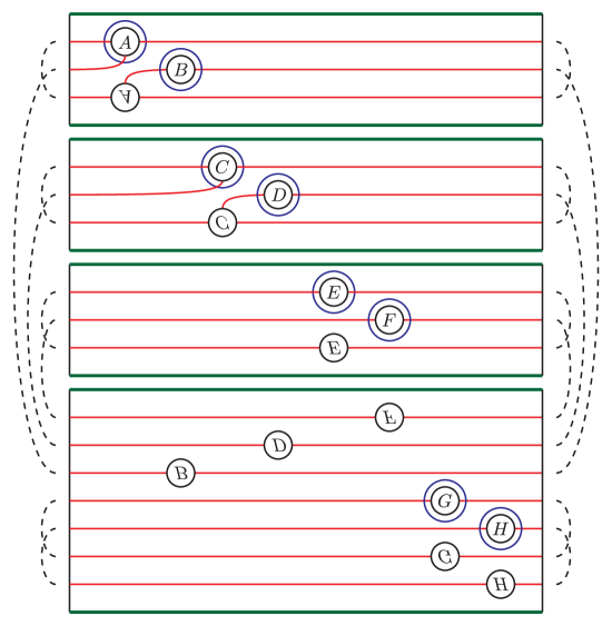
Figure 11. Bordered-sutured Heegaard diagram for $\boldsymbol{\tau}$. The case shown has $\partial Y$ of genus $1$ and $\ell=2$. Note that this diagram is a destabilization of the composition of the standard Heegaard diagrams for two arcslides.

Theorem 7.29 gives a way of computing the bimodule $\boldsymbol{\tau}$, resolving difficulty (🌧2). Explicitly, if the boundary of $Y$ has genus $k$ and $T$ consists of $\ell$ arcs and some number of circles then, for an appropriate choice of arc diagram we can factor $\boldsymbol{\tau}$ as a product of $\ell$ arcslides; see Figure 11. So, the bimodule for $\boldsymbol{\tau}$ is straightforward to compute from Proposition 7.18 and Corollary 7.17.

7.2. Evading the Novikov ring

Next we turn to difficulty (🌧3). The idea is to replace the Novikov ring $\Lambda$ with the field of rational functions $\mathbb{F}_{2}(x_{1},\dots,x_{4k-1})$, over which computing the homology of chain complexes is clearly algorithmic, and ${}^{\mathcal{A}(\mathcal{Z})}\mskip-1.80002mu\mathbf{\Lambda}(\mathcal{Z})_{\mathcal{A}(\mathcal{Z})}$ by a type $\mathit{DA}$ bimodule ${}^{\mathcal{A}(\mathcal{Z})}\mskip-1.80002mu\mathit{FoF}(\mathcal{Z})_{\mathcal{A}(\mathcal{Z})}$. Before definition $\mathit{FoF}$, note that there is an embedding $\nu\nobreak\mskip 2.0mu\mathpunct{}\nonscript\mkern-3.0mu{:}\penalty 300\mskip 6.0mu plus 1.0mu\mathbb{Z}^{4k-1}\hookrightarrow\mathbb{F}_{2}(x_{1},\dots,x_{4k-1})^{\times}$ given by

$$\nu(a_{1},\dots,a_{4k-1})=x_{1}^{a_{1}}\cdots x_{4k-1}^{a_{4k-1}}.$$

Definition 7.30.

As a $\mathbb{F}_{2}(x_{1},\dots,x_{4k-1})\otimes_{\mathbb{F}_{2}}\mathcal{I}(\mathcal{Z})$-module, define

$$\mathit{FoF}(\mathcal{Z})=\mathbb{F}_{2}(x_{1},\dots,x_{4k-1})\otimes_{\mathbb{F}_{2}}\mathcal{I}(\mathcal{Z}).$$

The structure maps $\delta^{1}_{n}$ on $\mathit{FoF}(\mathcal{Z})$ are defined to vanish if $n\neq 2$, and $\delta^{1}_{2}\nobreak\mskip 2.0mu\mathpunct{}\nonscript\mkern-3.0mu{:}\penalty 300\mskip 6.0mu plus 1.0mu\mathit{FoF}(\mathcal{Z})\otimes\mathcal{A}(\mathcal{Z})\to\mathcal{A}(\mathcal{Z})\otimes\mathit{FoF}(\mathcal{Z})$ is a homomorphism of $\mathbb{F}_{2}(x_{1},\dots,x_{4k-1})$-vector spaces. So, it only remains to define $\delta^{1}(i\otimes a)$ for $i$ a basic idempotent (viewed as a generator of $\mathit{FoF}(\mathcal{Z})$) and $a$ a strand diagram. Define

$$\delta^{1}_{2}(i\otimes a)=\begin{cases}a\otimes\nu([a])j&\text{if }ia\neq 0,\text{ where }aj\neq 0\\ 0&\text{otherwise}.\end{cases}$$

Theorem 7.31.

Theorems 1.3 and 1.8 hold with ${}^{\mathcal{A}(\mathcal{Z})}\mskip-1.80002mu\mathbf{\Lambda}(\mathcal{Z})_{\mathcal{A}(\mathcal{Z})}$ replaced by ${}^{\mathcal{A}(\mathcal{Z})}\mskip-1.80002mu\mathit{FoF}(\mathcal{Z})_{\mathcal{A}(\mathcal{Z})}$.

Proof.

The map $\psi$ induces an injection $\mathbb{F}_{2}(x_{1},\dots,x_{4k-1})\hookrightarrow\Lambda$, and

$${}^{\mathcal{A}(\mathcal{Z})}\mskip-1.80002mu\mathbf{\Lambda}(\mathcal{Z})_{\mathcal{A}(\mathcal{Z})}\cong{}^{\mathcal{A}(\mathcal{Z})}\mskip-1.80002mu\mathit{FoF}(\mathcal{Z})_{\mathcal{A}(\mathcal{Z})}\otimes_{\mathbb{F}_{2}(x_{1},\dots,x_{4k-1})}\Lambda.$$

So, the result follows from the fact that, over a field, tensor product is an exact functor. ∎

A somewhat improved version of the bordered algorithm for computing $\widehat{\mathit{CFD}}(Y)$ has been implemented by Zhan [Zha]. Although we have not done so, it should be relatively straightforward to extend his code to give a computer program for checking incompressibility.

References

- [Aur10] Denis Auroux, Fukaya categories of symmetric products and bordered Heegaard-Floer homology, J. Gökova Geom. Topol. GGT 4 (2010), 1–54, arXiv:1001.4323.
- [Ben10] Alex James Bene, A chord diagrammatic presentation of the mapping class group of a once bordered surface, Geom. Dedicata 144 (2010), 171–190, arXiv:0802.2747.
- [CGH12a] Vincent Colin, Paolo Ghiggini, and Ko Honda, The equivalence of Heegaard Floer homology and embedded contact homology III: from hat to plus, 2012, arXiv:1208.1526.
- [CGH12b] by same author, The equivalence of Heegaard Floer homology and embedded contact homology via open book decompositions I, 2012, arXiv:1208.1074.
- [CGH12c] by same author, The equivalence of Heegaard Floer homology and embedded contact homology via open book decompositions II, 2012, arXiv:1208.1077.
- [Gil16] Thomas J. Gillespie, L-space fillings and generalized solid tori, 2016, arXiv:1603.05016.
- [GL15] Paolo Ghiggini and Paolo Lisca, Open book decompositions versus prime factorizations of closed, oriented 3-manifolds, Interactions between low-dimensional topology and mapping class groups, Geom. Topol. Monogr., vol. 19, Geom. Topol. Publ., Coventry, 2015, pp. 145–155.
- [Hak68] Wolfgang Haken, Some results on surfaces in -manifolds, Studies in Modern Topology, Math. Assoc. Amer. (distributed by Prentice-Hall, Englewood Cliffs, N.J.), 1968, pp. 39–98.
- [Han16] Jonathan Hanselman, Bordered Heegaard Floer homology and graph manifolds, Algebr. Geom. Topol. 16 (2016), no. 6, 3103–3166.
- [HLW17] Jennifer Hom, Tye Lidman, and Liam Watson, The Alexander module, Seifert forms, and categorification, J. Topol. 10 (2017), no. 1, 22–100.
- [HN10] Matthew Hedden and Yi Ni, Manifolds with small Heegaard Floer ranks, Geom. Topol. 14 (2010), no. 3, 1479–1501.
- [HN13] by same author, Khovanov module and the detection of unlinks, Geom. Topol. 17 (2013), no. 5, 3027–3076.
- [Juh06] András Juhász, Holomorphic discs and sutured manifolds, Algebr. Geom. Topol. 6 (2006), 1429–1457, arXiv:math/0601443.
- [Juh08] by same author, Floer homology and surface decompositions, Geom. Topol. 12 (2008), no. 1, 299–350, arXiv:math/0609779.
- [KLT10a] Çağatay Kutluhan, Yi-Jen Lee, and Clifford Henry Taubes, I: Heegaard Floer homology and Seiberg–Witten Floer homology, 2010, arXiv:1007.1979.
- [KLT10b] by same author, II: Reeb orbits and holomorphic curves for the ech/Heegaard-Floer correspondence, 2010, 1008.1595.
- [KLT10c] by same author, III: Holomorphic curves and the differential for the ech/Heegaard Floer correspondence, 2010, arXiv:1010.3456.
- [KLT11] by same author, IV: The Seiberg-Witten Floer homology and ech correspondence, 2011, arXiv:1107.2297.
- [KLT12] Çağatay Kutluhan, Yi-Jen Lee, and Clifford Henry Taubes, V: Seiberg-Witten Floer homology and handle additions, 2012, arXiv:1204.0115.
- [LOT08] Robert Lipshitz, Peter S. Ozsváth, and Dylan P. Thurston, Bordered Heegaard Floer homology: Invariance and pairing, 2008, arXiv:0810.0687v4.
- [LOT11] Robert Lipshitz, Peter S. Ozsváth, and Dylan P. Thurston, Heegaard Floer homology as morphism spaces, Quantum Topol. 2 (2011), no. 4, 381–449, arXiv:1005.1248.
- [LOT14] Robert Lipshitz, Peter S. Ozsváth, and Dylan P. Thurston, Computing by factoring mapping classes, Geom. Topol. 18 (2014), no. 5, 2547–2681.
- [LOT15] Robert Lipshitz, Peter S. Ozsváth, and Dylan P. Thurston, Bimodules in bordered Heegaard Floer homology, Geom. Topol. 19 (2015), no. 2, 525–724.
- [LT16] Robert Lipshitz and David Treumann, Noncommutative Hodge-to-de Rham spectral sequence and the Heegaard Floer homology of double covers, J. Eur. Math. Soc. (JEMS) 18 (2016), no. 2, 281–325.
- [Ni09] Yi Ni, Heegaard Floer homology and fibred 3-manifolds, Amer. J. Math. 131 (2009), no. 4, 1047–1063.
- [Ni13] by same author, Nonseparating spheres and twisted Heegaard Floer homology, Algebr. Geom. Topol. 13 (2013), no. 2, 1143–1159.
- [OSz04a] Peter S. Ozsváth and Zoltán Szabó, Holomorphic disks and genus bounds, Geom. Topol. 8 (2004), 311–334.
- [OSz04b] by same author, Holomorphic disks and three-manifold invariants: properties and applications, Ann. of Math. (2) 159 (2004), no. 3, 1159–1245, arXiv:math.SG/0105202.
- [OSz04c] by same author, Holomorphic disks and topological invariants for closed three-manifolds, Ann. of Math. (2) 159 (2004), no. 3, 1027–1158, arXiv:math.SG/0101206.
- [Pen87] R. C. Penner, The decorated Teichmüller space of punctured surfaces, Comm. Math. Phys. 113 (1987), no. 2, 299–339.
- [Sha98] V. V. Sharko, Functions on surfaces. I, Some problems in contemporary mathematics (Russian), Pr. Inst. Mat. Nats. Akad. Nauk Ukr. Mat. Zastos., vol. 25, Natsīonal. Akad. Nauk Ukraïni, Īnst. Mat., Kiev, 1998, pp. 408–434.
- [Tau10a] Clifford Henry Taubes, Embedded contact homology and Seiberg-Witten Floer cohomology I, Geom. Topol. 14 (2010), no. 5, 2497–2581.
- [Tau10b] by same author, Embedded contact homology and Seiberg-Witten Floer cohomology II, Geom. Topol. 14 (2010), no. 5, 2583–2720.
- [Tau10c] by same author, Embedded contact homology and Seiberg-Witten Floer cohomology III, Geom. Topol. 14 (2010), no. 5, 2721–2817.
- [Tau10d] by same author, Embedded contact homology and Seiberg-Witten Floer cohomology IV, Geom. Topol. 14 (2010), no. 5, 2819–2960.
- [Tau10e] by same author, Embedded contact homology and Seiberg-Witten Floer cohomology V, Geom. Topol. 14 (2010), no. 5, 2961–3000.
- [Zar09] Rumen Zarev, Bordered Floer homology for sutured manifolds, 2009, arXiv:0908.1106.
- [Zar10] by same author, Joining and gluing sutured Floer homology, 2010, arXiv:1010.3496.
- [Zha] Bohua Zhan, bfhpython, github.com/bzhan/bfhpython.