Introducing the truly chaotic finite state machines and theirs applications in security field

Abstract

The truly chaotic finite machines introduced by authors in previous research papers are presented here. A state of the art in this discipline, encompassing all previous mathematical investigations, is provided, explaining how finite state machines can behave chaotically regarding the slight alteration of their inputs. This behavior is explained using Turing machines and formalized thanks to a special family of discrete dynamical systems called chaotic iterations. An illustrative example is finally given in the field of hash functions.

1 Introduction

The use of chaotic dynamics in cryptography is often disputed as a finite state machine is reputed to always enter into a cycle. Even though such a regular behavior is not completely opposed to almost all definitions of chaos in mathematics, constituting a kind of border situation in case of discrete sets, this situation appears as problematic to cryptologists that consider periodic dynamics and chaos as antithetical. This problem can be solved by introducing truly chaotic finite machines. A second situation where such chaotic machines can serve is in the numerical simulations of chaotic real phenomena. Iterating chaotic dynamical systems of the real line on finite state machines leads to truncated sequences. It is possible to show that such periodic orbits of truncated terms are as close as possible to truly chaotic real ones via the shadow lemma. However the orbit that is approximated by the finite machine has a initial condition with a priori no relation with the targeted one.

Our proposal is to constitute truly chaotic finite machines, that is, finite machines that can be rigorously proven as chaotic, as defined by Devaney [5], Knudsen [8], and so on. The key idea is to consider that the finite machine is not separated from the outside world but that it must interact with it in order to be useful. At each iteration, the new input provided to the finite machine can be used together with its current state to produce the next output. By doing so, the finite machine iterates on the finite cartesian product of its possible states multiply by all the possible inputs. The machine can be written as an iterative process, thus it still remains to study the behavior of outputs on slight modifications on the inputs. After having recalled the various existing notions of chaos in mathematical topology, this idea is formalized theoretically using Turing machines and explained practically thanks to the so-called chaotic iterations. An example of use is finally provided in the field of hash functions.

The remainder of this research work, which summarizes our recent discoveries in truly chaotic finite machines and theirs applications, is organized as follows.

2 The Mathematical Theory of Chaos

In the whole document, to prevent from any conflicts and to avoid unreadable writings, we have considered the following notations, usually in use in discrete mathematics:

• The $n-$th term of the sequence $s$ is denoted by $s^{n}$.

• The $i-$th component of vector $v$ is $v_{i}$.

• The $k-$th composition of function $f$ is denoted by $f^{k}$. Thus $f^{k}=f\circ f\circ\ldots\circ f$, $k$ times.

• The derivative of $f$ is $f^{\prime}$.

$\mathcal{P}(X)$ is the set of subsets of $X$. On the other hand $\mathds{B}$ stands for the set $\{0;1\}$ with its usual algebraic structure (Boolean addition, multiplication, and negation), while $\mathds{N}$ and $\mathds{R}$ are the usual notations of the following respective sets: natural numbers and real numbers. $\mathcal{X}^{\mathcal{Y}}$ is the set of applications from $\mathcal{Y}$ to $\mathcal{X}$, and thus $\mathcal{X}^{\mathds{N}}$ means the set of sequences belonging in $\mathcal{X}$. We will use the notation $\lfloor x\rfloor$ for the integral part of a real $x$, that is, the greatest integer lower than $x$. Finally, $\llbracket a;b\rrbracket=\{a,a+1,\ldots,b\}$ is the set of integers between $a$ and $b$.

In this section are presented various understanding of a chaotic behavior for a discrete dynamical system.

2.1 Approaches similar to Devaney

In these approaches, three ingredients are required for unpredictability [6]. Firstly, the system must be intrinsically complicated, undecomposable: it cannot be simplified into two subsystems that do not interact, making any divide and conquer strategy applied to the system inefficient. In particular, a lot of orbits must visit the whole space. Secondly, an element of regularity is added, to counteract the effects of the first ingredient, leading to the fact that closed points can behave in a completely different manner, and this behavior cannot be predicted. Finally, sensibility of the system is demanded as a third ingredient, making that close points can finally become distant during iterations of the system. This last requirement is, indeed, often implied by the two first ingredients. Having this understanding of an unpredictable dynamical system, Devaney has formalized in [5] the following definition of chaos.

Definition 1.

A discrete dynamical system $x^{0}\in\mathcal{X},x^{n+1}=f(x^{n})$ on a metric space $(\mathcal{X},d)$ is chaotic according to Devaney if:

1. Transitivity: For each couple of open sets $A,B\subset\mathcal{X}$, there exists $\exists k\in\mathbb{N}$ such that $f^{k}(A)\cap B\neq\varnothing$.

2. Regularity: Periodic points are dense in $\mathcal{X}$.

3. Sensibility to the initial conditions: There exists $\varepsilon>0$ such that

   $$\forall x\in\mathcal{X},\forall\delta>0,\exists y\in\mathcal{X},\exists n\in\mathbb{N},d(x,y)<\delta\textrm{ and }d(f^{n}(x),f^{n}(y))\geqslant\varepsilon.$$

The system can be intrinsically complicated for various other understanding of this wish, that are not equivalent one another, like:

• Undecomposable: it is not the union of two nonempty closed subsets that are positively invariant ($f(A)\subset A$).

• Total transitivity: $\forall n\geqslant 1$, the function composition $f^{n}$ is transitive.

• Strong transitivity: $\forall x,y\in\mathcal{X},$ $\forall r>0,$ $\exists z\in B(x,r),$ $\exists n\in\mathbb{N},$ $f^{n}(z)=y.$

• Topological mixing: for all pairs of disjoint open nonempty sets $U$ and $V$, there exists $n_{0}\in\mathbb{N}$ such that $\forall n\geqslant n_{0},f^{n}(U)\cap V\neq\varnothing$.

Concerning the ingredient of sensibility, it can be reformulated as follows.

• $(\mathcal{X},f)$ is unstable is all its points are unstable: $\forall x\in\mathcal{X},$ $\exists\varepsilon>0,$ $\forall\delta>0,$ $\exists y\in\mathcal{X},$ $\exists n\in\mathbb{N},$ $d(x,y)<\delta$ and $d(f^{n}(x),f^{n}(y))\geqslant\varepsilon$.

• $(\mathcal{X},f)$ is expansive is $\exists\varepsilon>0,$ $\forall x\neq y,$ $\exists n\in\mathbb{N},$ $d(f^{n}(x),f^{n}(y))\geqslant\varepsilon$

These varieties of definitions lead to various notions of chaos. For instance, a dynamical system is chaotic according to Wiggins if it is transitive and sensible to the initial conditions. It is said chaotic according to Knudsen if it has a dense orbit while being sensible. Finally, we speak about expansive chaos when the properties of transitivity, regularity, and expansiveness are satisfied.

2.2 Li-Yorke approach

The approach for chaos presented in the previous section, considering that a chaotic system is a system intrinsically complicated (undecomposable), with possibly an element of regularity and/or sensibility, has been completed by other understanding of chaos. Indeed, as “randomness” or “infinity”, a single universal definition of chaos cannot be found. The kind of behaviors that are attempted to be described are too much complicated to enter into only one definition. Instead, a large panel of mathematical descriptions have been proposed these last decades, being all theoretically justified. Each of these definitions give illustration to some particular aspects of a chaotic behavior.

The first of these parallel approaches can be found in the pioneer work of Li and Yorke [9]. In their well-known article entitled “Period three implies chaos”, they rediscovered a weaker formulation of the Sarkovskii’s theorem, meaning that when a discrete dynamical system $(f,[0,1])$, with $f$ continuous, has a 3-cycle, then it has too a $n-$cycle, $\forall n\leqslant 2$. The community has not adopted this definition of chaos, as several degenerated systems satisfy this property. However, on their article [9], Li and Yorke have studied too another interesting property, which has led to a notion of chaos “according to Li and Yorke” recalled below.

Definition 2.

Let $(\mathcal{X},d)$ a metric space and $f:\mathcal{X}\longrightarrow\mathcal{X}$ a continuous map. $(x,y)\in\mathcal{X}^{2}$ is a scrambled couple of points if $\liminf_{n\rightarrow\infty}d(f^{n}(x),f^{n}(y))=0$ and $\limsup_{n\rightarrow\infty}d(f^{n}(x),f^{n}(y))>0$: the two orbits oscillate.

A scrambled set is a set in which any couple of points are a scrambled couple, whereas a Li-Yorke chaotic system is a system possessing an uncountable scrambled set.

2.3 Topological entropy approach

Let $f:\mathcal{X}\longrightarrow\mathcal{X}$ be a continuous map on a compact metric space $(\mathcal{X},d)$. For each natural number $n$, a new metric $d_{n}$ is defined on $\mathcal{X}$ by

$$d_{n}(x,y)=\max\{d(f^{i}(x),f^{i}(y)):0\leq i<n\}.$$

Given any $\varepsilon>0$ and $n\geqslant 1$, two points of $\mathcal{X}$ are $\varepsilon$-close with respect to this metric if their first $n$ iterates are $\varepsilon$-close. This metric allows one to distinguish in a neighborhood of an orbit the points that move away from each other during the iteration from the points that travel together. A subset $E$ of $\mathcal{X}$ is said to be $(n,\varepsilon)$-separated if each pair of distinct points of $E$ is at least $\varepsilon$ apart in the metric $d_{n}$. Denote by $N(n,\varepsilon)$ the maximum cardinality of a $(n,\varepsilon)$-separated set. $N(n,\varepsilon)$ represents the number of distinguishable orbit segments of length $n$, assuming that we cannot distinguish points within $\varepsilon$ of one another.

Definition 3.

The topological entropy of the map $f$ is defined by

$$h(f)=\lim_{\epsilon\to 0}\left(\limsup_{n\to\infty}\frac{1}{n}\log N(n,\epsilon)\right).$$

The limit defining $h(f)$ may be interpreted as the measure of the average exponential growth of the number of distinguishable orbit segments. In this sense, it measures complexity of the topological dynamical system $(\mathcal{X},f)$.

2.4 The Lyapunov exponent

The last measure of chaos that will be regarded in this document is the Lyapunov exponent. This quantity characterizes the rate of separation of infinitesimally close trajectories. Indeed, two trajectories in phase space with initial separation $\delta$ diverge at a rate approximately equal to $\delta e^{\lambda t}$, where $\lambda$ is the Lyapunov exponent, which is defined by:

Definition 4.

Let $f:\mathds{R}\longrightarrow\mathds{R}$ be a differentiable function, and $x^{0}\in\mathds{R}$. The Lyapunov exponent is given by $\lambda(x^{0})=\displaystyle{\lim_{n\to+\infty}\dfrac{1}{n}\sum_{i=1}^{n}\ln\left|~{}f^{\prime}\left(x^{i-1}\right)\right|}.$

Obviously, this exponent must be positive to have a multiplication of the initial errors by an exponentially increasing factor, and thus chaos in this understanding.

3 The So-called Chaotic Iterations

Our proposal in creating chaotic finite machines is to take a new input at each iteration. This process can be realized using a tool called chaotic iterations.

3.1 Introducing chaotic iterations

Definition 5.

Let $f:\mathds{B}^{\mathsf{N}}\longrightarrow\mathds{B}^{\mathsf{N}}$ and $S\in\mathcal{P}\left(\llbracket 1,\mathsf{N}\rrbracket\right)^{\mathds{N}}$. Chaotic iterations $(f,(x^{0},S))$ are defined by:

$$\left\{\begin{array}[]{l}x^{0}\in\mathds{B}^{\mathsf{N}}\\ \forall n\in\mathds{N}^{*},\forall i\in\llbracket 1;\mathsf{N}\rrbracket,x^{n}_{i}=\left\{\begin{array}[]{ll}x^{n-1}_{i}&\textrm{ if }i\notin S^{n}\\ f(x^{n-1})_{i}&\textrm{ if }i\in S^{n}\end{array}\right.\end{array}\right.$$

A priori, there is no relation between these chaotic iterations and the mathematical theory of chaos recalled in the previous section. On our side, we have regarded whether these chaotic iterations can behave chaotically, as it is defined for instance by Devaney, and if so, in which application context this behavior can be profitable. To do so, chaotic iterations have first been rewritten as simple discrete dynamical systems, as follows.

3.2 Chaotic Iterations as Dynamical Systems

To realize the junction between the two frameworks presented previously, the following material can be introduced [4]:

• the shift function: $\sigma:\mathcal{S}\longrightarrow\mathcal{S},(S^{n})_{n\in\mathds{N}}\mapsto(S^{n+1})_{n\in\mathds{N}}$.

• the initial function, defined by $i:\mathcal{S}\longrightarrow\llbracket 1;\mathsf{N}\rrbracket,(S^{n})_{n\in\mathds{N}}\mapsto S^{0}$

• and $F_{f}:\llbracket 1;\mathsf{N}\rrbracket\times\mathds{B}^{\mathsf{N}}\longrightarrow\mathds{B}^{\mathsf{N}},$

  $$(k,E)\longmapsto\left(E_{j}.\delta(k,j)+f(E)_{k}.\overline{\delta(k,j)}\right)_{j\in\llbracket 1;\mathsf{N}\rrbracket}$$

where $\delta$ is the discrete metric.

Let $\mathcal{X}=\llbracket 1;\mathsf{N}\rrbracket^{\mathds{N}}\times\mathds{B}^{\mathsf{N}},$ and $G_{f}\left(S,E\right)=\left(\sigma(S),F_{f}(i(S),E)\right).$ Chaotic iterations $\left(f,(S,x^{0})\right)$ can be modeled by the discrete dynamical system:

$$\left\{\begin{array}[]{l}X^{0}=(S,x^{0})\in\mathcal{X},\\ \forall k\in\mathds{N},X^{k+1}=G_{f}(X^{k}).\end{array}\right.$$

Their topological disorder can then be studied. To do so, a relevant distance must be defined on $\mathcal{X}$, as follows [7]:

$$d((S,E);(\check{S};\check{E}))=d_{e}(E,\check{E})+d_{s}(S,\check{S})$$

where $\displaystyle{d_{e}(E,\check{E})=\sum_{k=1}^{\mathsf{N}}\delta(E_{k},\check{E}_{k})}$,   and  $\displaystyle{d_{s}(S,\check{S})=\dfrac{9}{\textsf{N}}\sum_{k=1}^{\infty}\dfrac{|S^{k}-\check{S}^{k}|}{10^{k}}}$.

This new distance has been introduced to satisfy the following requirements.

• When the number of different cells between two systems is increasing, then their distance should increase too.

• In addition, if two systems present the same cells and their respective strategies start with the same terms, then the distance between these two points must be small because the evolution of the two systems will be the same for a while. Indeed, the two dynamical systems start with the same initial condition, use the same update function, and as strategies are the same for a while, then components that are updated are the same too.

The distance presented above follows these recommendations. Indeed, if the floor value $\lfloor d(X,Y)\rfloor$ is equal to $n$, then the systems $E,\check{E}$ differ in $n$ cells. In addition, $d(X,Y)-\lfloor d(X,Y)\rfloor$ is a measure of the differences between strategies $S$ and $\check{S}$. More precisely, this floating part is less than $10^{-k}$ if and only if the first $k$ terms of the two strategies are equal. Moreover, if the $k^{th}$ digit is nonzero, then the $k^{th}$ terms of the two strategies are different. It can then be stated that

Proposition 1.

$G_{f}:(\mathcal{X},d)\to(\mathcal{X},d)$ is a continuous function

With all this material, the study of chaotic iterations as a discrete dynamical system has then be realized. The topological space on which chaotic iterations are defined has firstly been investigated, leading to the following result [7]:

Proposition 2.

$\mathcal{X}$ is an infinitely countable metric space, being both compact, complete, and perfect (each point is an accumulation point).

These properties are required in some topological specific formalization of a chaotic dynamical system, justifying their proofs. Concerning $G_{f_{0}}$, it has been stated that [7].

Proposition 3.

$G_{f_{0}}$ is surjective, but not injective, and so the dynamical system $(\mathcal{X},G_{f_{0}})$ is not reversible.

It is now possible to recall the topological behavior of chaotic iterations.

3.3 The Study of Iterative Systems

We have firstly stated that [7]:

Theorem 1.

$G_{f_{0}}$ is regular and transitive on $(\mathcal{X},d)$, thus it is chaotic according to Devaney. Furthermore, its constant of sensibility is greater than $\mathsf{N}-1$.

Thus the set $\mathcal{C}$ of functions $f:\mathds{B}^{\mathsf{N}}\longrightarrow\mathds{B}^{\mathsf{N}}$ making the chaotic iterations of Definition 5 a case of chaos according to Devaney, is a nonempty set. To characterize functions of $\mathcal{C}$, we have firstly stated that transitivity implies regularity for these particular iterated systems [3]. To achieve characterization, we then have introduced the following graph.

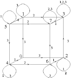
Figure 1: Example of an asynchronous iteration graph

Let $f$ be a map from $\mathds{B}^{\mathsf{N}}$ to itself. The asynchronous iteration graph associated with $f$ is the directed graph $\Gamma(f)$ defined by: the set of vertices is $\mathds{B}^{\mathsf{N}}$; for all $x\in\mathds{B}^{\mathsf{N}}$ and $i\in\llbracket 1;\mathsf{N}\rrbracket$, the graph $\Gamma(f)$ contains an arc from $x$ to $F_{f}(i,x)$. The relation between $\Gamma(f)$ and $G_{f}$ is clear: there exists a path from $x$ to $x^{\prime}$ in $\Gamma(f)$ if and only if there exists a strategy $s$ such that the parallel iteration of $G_{f}$ from the initial point $(s,x)$ reaches the point $x^{\prime}$. Figure 1 presents such an asynchronous iteration graph. We thus have proven that [3].

Theorem 2.

$G_{f}$ is transitive, and thus chaotic according to Devaney, if and only if $\Gamma(f)$ is strongly connected.

This characterization makes it possible to quantify the number of functions in $\mathcal{C}$: it is equal to $\left(2^{\mathsf{N}}\right)^{2^{\mathsf{N}}}$. Then the study of the topological properties of disorder of these iterative systems has been further investigated, leading to the following results.

Theorem 3.

$\forall f\in\mathcal{C}$, $Per\left(G_{f}\right)$ is infinitely countable, $G_{f}$ is strongly transitive and is chaotic according to Knudsen. It is thus undecomposable, unstable, and chaotic as defined by Wiggins.

Theorem 4.

$\left(\mathcal{X},G_{f_{0}}\right)$ is topologically mixing, expansive (with a constant equal to 1), chaotic as defined by Li and Yorke, and has a topological entropy and an exponent of Lyapunov both equal to $ln(\mathsf{N})$.

At this stage, a new kind of iterative systems that only manipulates integers have been discovered, leading to the questioning of their computing for security applications. In order to do so, the possibility of their computation without any loss of chaotic properties has first been investigated. These chaotic machines are presented in the next section.

4 Chaotic Turing Machines

4.1 General presentation

Let us consider a given algorithm. Because it must be computed one day, it is always possible to translate it as a Turing machine, and this last machine can be written as $x^{n+1}=f(x^{n})$ in the following way. Let $(w,i,q)$ be the current configuration of the Turing machine (Figure 2), where $w=\sharp^{-\omega}w(0)\ldots w(k)\sharp^{\omega}$ is the paper tape, $i$ is the position of the tape head, $q$ is used for the state of the machine, and $\delta$ is its transition function (the notations used here are well-known and widely used). We define $f$ by:

• $f(w(0)\ldots w(k),i,q)=(w(0)\ldots w(i-1)aw(i+1)w(k),i+1,q^{\prime})$, if $\delta(q,w(i))=(q^{\prime},a,\rightarrow)$,

• $f(w(0)\ldots w(k),i,q)=(w(0)\ldots w(i-1)aw(i+1)w(k),i-1,q^{\prime})$, if $\delta(q,w(i))=(q^{\prime},a,\leftarrow)$.

Thus the Turing machine can be written as an iterate function $x^{n+1}=f(x^{n})$ on a well-defined set $\mathcal{X}$, with $x^{0}$ as the initial configuration of the machine. We denote by $\mathcal{T}(S)$ the iterative process of the algorithm $S$.

Figure 2: Turing Machine

Let $\tau$ be a topology on $\mathcal{X}$. So the behavior of this dynamical system can be studied to know whether or not the algorithm is $\tau$-chaotic. Let us now explain how it is possible to have true chaos in a finite state machine.

4.2 Practical Issues

Up to now, most of computer programs presented as chaotic lose their chaotic properties while computing in the finite set of machine numbers. The algorithms that have been presented as chaotic usually act as follows. After having received its initial state, the machine works alone with no interaction with the outside world. Its outputs only depend on the different states of the machine. The main problem which prevents speaking about chaos in this particular situation is that when a finite state machine reaches the same internal state twice, the two future evolution are identical. Such a machine always finishes by entering into a cycle while iterating. This highly predictable behavior cannot be set as chaotic, at least as expressed by Devaney. Some attempts to define a discrete notion of chaos have been proposed, but they are not completely satisfactory and are less recognized than the notions exposed in a previous section.

The next stage was then to prove that chaos is possible in finite machine. The two main problems are that: (1) Chaotic sequences are usually defined in the real line whereas define real numbers on computers is impossible. (2) All finite state machines always enter into a cycle when iterating, and this periodic behavior cannot be stated as chaotic.

The first problem is disputable, as the shadow lemma proves that, when considering the sequence $x^{n+1}=trunc_{k}\left(f(x^{n})\right)$, where $(f,[0,1])$ is a chaotic dynamical system and $trunc_{k}(x)=\dfrac{\lfloor 10^{k}x\rfloor}{10^{k}}$ is the truncated version of $x\in\mathds{R}$ at its $k-$th digits, then the sequence $(x^{n})$ is as close as possible to a real chaotic orbit. Thus iterating a chaotic function on floating point numbers does not deflate the chaotic behavior as much. However, even if this first claim is not really a problem, we have prevent from any disputation by considering a tool (the chaotic iterations) that only manipulates integers bounded by $\mathsf{N}$.

The second claim is surprisingly never considered as an issue when considering the generation of randomness on computers. However, the stated problem can be solved in the following way. The computer must generate an output $O$ computed from its current state $E$ and the current value of an input $S$, which changes at each iteration (Figure 3). Therefore, it is possible that the machine presents the same state twice, but with two future evolution completely different, depending on the values of the input. By doing so, we thus obtain a machine with a finite number of states, which can evolve in infinitely different ways, due to the new values provided by the input at each iteration. Thus such a machine can behave chaotically.

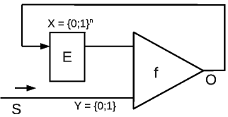
Figure 3: A chaotic finite-state machine. At each iteration, a new value is taken from the outside world (S). It is used by f as input together with the current state (E).

5 Application to Hash Functions

5.1 Definitions

This section is devoted to a concrete realization of such a finite state chaotic machine in the computer science security field. We will show that, given a secured hash function, it is possible to realize a post-treatment on the obtained digest using chaotic iterations that preserves the security of the hash function. Furthermore, if the media to hash is obtained frame by frame from a stream, the resulted hash machine inherits the chaos properties of the chaotic iterations presented previously. For the interest to add chaos properties to an hash function, among other things regarding their diffusion and confusion [10], reader is referred to the following experimental studies: [1, 7, 2].

Let us firstly introduce some definitions.

Definition 6 (Keyed One-Way Hash Function).

Let $\Gamma$ and $\Sigma$ be two alphabets, let $k\in K$ be a key in a given key space, let $l$ be a natural numbers which is the length of the output message, and let $h:K\times\Gamma^{+}\rightarrow\Sigma^{l}$ be a function that associates a message in $\Sigma^{l}$ for each pair of key, word in $K\times\Gamma^{+}$. The set of all functions $h$ is partitioned into classes of functions $\{h_{k}:k\in K\}$ indexed by a key $k$ and such that $h_{k}:\Gamma^{+}\rightarrow\Sigma^{l}$ is defined by $h_{k}(m)=h(k,m)$, i.e., $h_{k}$ generates a message digest of length $l$.

Definition 7 (Collision resistance).

For a keyed hash function $h:\mathds{B}^{k}\times\mathds{B}^{*}\longrightarrow\mathds{B}^{n}$, define the advantage of an adversary $\mathsf{A}$ for finding a collision as

$$Adv_{\mathsf{A}}=Pr\left[\begin{array}[]{c}K\xleftarrow{\$}\mathds{B}^{k}\\ (m,m^{\prime})\leftarrow\mathsf{A}(K)\end{array}:\begin{array}[]{c}m\neq m^{\prime}\\ h(K,m)=h(K,m^{\prime})\end{array}\right]$$ (1)

where $\$$ means that the element is pick randomly. The insecurity of $h$ with respect to collision resistance is

$$InSec_{h}(t)=\max_{\mathsf{A}}\left\{Adv_{\mathsf{A}}\right\}$$ (2)

when the maximum is taken over all adversaries $\mathsf{A}$ with total running time $t$.

In other words, an adversary should not be able to find a collision, that is, two distinct messages $m$ and $m^{\prime}$ such that $h(m)=h(m^{\prime})$.

Definition 8 (Second-Preimage Resistance).

For a keyed hash function $h:\mathds{B}^{k}\times\mathds{B}^{*}\longrightarrow\mathds{B}^{n}$, define the advantage of an adversary $\mathsf{A}$ for finding a second-preimage as

$$Adv_{\mathsf{A}}(m)=Pr\left[\begin{array}[]{c}K\xleftarrow{\$}\mathds{B}^{k}\\ m^{\prime}\xleftarrow{\$}\mathsf{A}(K)\end{array}:\begin{array}[]{c}m\neq m^{\prime}\\ h(K,m)=h(K,m^{\prime})\end{array}\right]$$ (3)

The insecurity of $h$ with respect to collision resistance is

$$InSec_{h}(t)=\max_{\mathsf{A}}\left\{\max_{m\in\mathds{B}^{k}}\left\{Adv_{\mathsf{A}}(m)\right\}\right\}$$ (4)

when the maximum is taken over all adversaries $\mathsf{A}$ with total running time $t$.

That is to say, an adversary given a message $m$ should not be able to find another message $m^{\prime}$ such that $m\neq m^{\prime}$ and $h(m)=h(m^{\prime})$. Let us now give a post-operative mode that can be applied to a cryptographically secure hash function without loosing the cryptographic properties recalled above.

Definition 9.

Let

• $k_{1},k_{2},n\in\mathds{N}^{*}$,

• $h:(k,m)\in\mathds{B}^{k_{1}}\times\mathds{B}^{*}\longmapsto h(k,m)\in\mathds{B}^{n}$ a keyed hash function,

• $S:k\in\mathds{B}^{k_{2}}\longmapsto\left(S(k)^{i}\right)_{i\in\mathds{N}}\in\llbracket 1,n\rrbracket^{\mathds{N}}$:

  • either a cryptographically secure pseudorandom number generator (PRNG),

  • or, in case of a binary input stream $m=m^{0}||m^{1}||m^{1}||\ldots$ where $\forall i,|m^{i}|=n$, $\left(S(k)^{i}\right)_{i\in\mathds{N}}=\left(m^{k}\right)_{i\in\mathds{N}}$.

• $\mathcal{K}=\mathds{B}^{k_{1}}\times\mathds{B}^{k_{2}}\times\mathds{N}$ called the key space,

• and $f:\mathds{B}^{n}\longrightarrow\mathds{B}^{n}$ a bijective map.

We define the keyed hash function $\mathcal{H}_{h}:\mathcal{K}\times\mathds{B}^{*}\longrightarrow\mathds{B}^{n}$ by the following procedure
Inputs: $k=(k_{1},k_{2},n)\in\mathcal{K}$ $m\in\mathds{B}^{*}$ Runs: $X=h(k_{1},m)$, or $X=h(k_{1},m^{0})$ if $m$ is a stream for $i=1,\ldots,n:$        $X=G_{f}(X,S^{i})$ return $X$

$\mathcal{H}_{h}$ is thus a chaotic iteration based post-treatment on the inputted hash function $h$. The strategy is provided by a secured PRNG when the machine operates in a vacuum whereas it is redetermined at each iteration from the input stream in case of a finite machine open to the outside. By doing so, we obtain a new hash function $\mathcal{H}_{h}$ with $h$, and this new one has a chaotic dependence regarding the inputted stream.

5.2 Security proofs

The two following lemma are obvious.

Lemma 1.

If $f:\mathds{B}^{n}\longrightarrow\mathds{B}^{n}$ is bijective, then $\forall S\in\llbracket 1,n\rrbracket$, the map $G_{f,S}:x\in\mathds{B}^{n}\rightarrow G_{f}(x,S)_{1}\in\mathds{B}^{n}$ is bijective too.

Proof.

Let $y=(y_{1},\ldots,y_{n})\in\mathds{B}^{n}$ and $S\in\llbracket 1,n\rrbracket$. Thus

$$G_{f,S}(y_{1},\ldots,y_{S-1},f^{-1}(y_{S}),y_{S+1},\ldots,y_{n})_{1}=y.$$

So $G_{f,S}$ is a surjective map between two finite sets. ∎

Lemma 2.

Let $S\in\llbracket 1,n\rrbracket^{\mathds{N}}$ and $N\in\mathds{N}^{*}$. If $f$ is bijective, then $G_{f,S,N}:x\in\mathds{B}^{n}\longmapsto G_{f}^{N}(x,S)_{1}\in\mathds{B}^{n}$ is bijective too.

Proof.

Indeed, $G_{s,f,n}=G_{f,S^{n}}\circ\ldots\circ G_{f,S^{0}}$ is bijective as a composition of bijective maps. ∎

We can now state that,

Theorem 5.

If $h$ satisfies the collision resistance property, then it is the case too for $\mathcal{H}_{h}$. And if $h$ satisfies the second-preimage resistance property, then it is the case too for $\mathcal{H}_{h}$.

Proof.

Let $A(k_{1},k_{2},n)=(m_{1},m_{2})$ such that $\mathcal{H}_{h}\left((k_{1},k_{2},n),m_{1}\right)=\mathcal{H}_{h}\left((k_{1},k_{2},n),m_{2}\right)$. Then $G_{f,S(k_{2}),n}\left(h(m_{1})\right)=G_{f,S(k_{2}),n}\left(h(m_{2})\right)$. So $h(m_{1},k_{1})=h(m_{2},k_{1})$.

For the second-preimage resistance property, let $m,k\in\mathds{B}^{*}\times\mathcal{K}$. If a message $m^{\prime}\in\mathds{B}^{*}$ can be found such that $\mathcal{H}_{h}(k,m)=\mathcal{H}_{h}(k,m^{\prime})$, then $h(k_{1},m)=h(k_{1},m^{\prime})$: a second-preimage for $h$ has thus be found. ∎

Finally, as $\mathcal{H}_{h}$ simply operates chaotic iterations with strategy $\mathcal{S}$ provided at each iterate by the media, we have:

Theorem 6.

In case where the strategy $\mathcal{S}$ is the bitwise xor between a secured PRNG and the input stream, the resulted hash function $\mathcal{H}_{h}$ is chaotic.

Remark 1.

$\mathcal{S}$ should be $m^{k}\oplus x^{k}$ where $(x^{k})$ is provided by a secured PRNG if security of $\mathcal{H}_{h}$ is required.

6 Conclusion

In this article, the research we have previously done in the field of truly chaotic finite machines are summarized and clarified to serve as an introduction to our approach. This approach consists in considering a specific family of discrete dynamical systems that iterate on a set having the form $\mathcal{X}=\mathcal{P}\left(\llbracket 1,N\rrbracket\right)^{\mathds{N}}\times\mathds{B}^{\mathds{N}}$, making it possible to obtain pure, non degenerated chaos on finite machines. These particular dynamical systems are called chaotic iterations. Our method consists in considering the left part of $\mathcal{X}$ as the tape of the Turing machine whereas the right part is the state register of the machine. Chaos implies here that if the initial tape and the initial state are not known exactly, then for some transition function the evolution of the iterates of the Turing machine, or in other words the evolution of the state register and of the tape, cannot be predicted. We remark too that the initial tape has not to be inputted integrally into the machine: it can be provided by, for instance, a video stream whose hash value is updated at each new received frame.

In our previous research papers, we have provided a necessary and sufficient condition on a Moore machine to behave as chaotic, this condition being the strong connectivity of an associated large graph. A sufficient condition of chaoticity on a smaller graph has been proven too. In future work, the authors’ intention is to extend these results to the Turing machines, to determine on which conditions on the transition function such machines have a stochastic behavior. Furthermore, only a special kind of Turing machines has been investigated until now, and the authors’ desire is to extend these results to all possible machines. A concrete chaotic machine should then be designed and studied. Finally new applications will be detailed.

References

- [1] Jacques Bahi, Jean-François Couchot, and Christophe Guyeux. Performance analysis of a keyed hash function based on discrete and chaotic proven iterations. In INTERNET 2011, the 3-rd Int. Conf. on Evolving Internet, pages 52–57, Luxembourg, Luxembourg, June 2011. Best paper award.
- [2] Jacques Bahi, Jean-François Couchot, and Christophe Guyeux. Quality analysis of a chaotic proven keyed hash function. International Journal On Advances in Internet Technology, 5(1):26–33, 2012.
- [3] Jacques Bahi, Jean-François Couchot, Christophe Guyeux, and Adrien Richard. On the link between strongly connected iteration graphs and chaotic boolean discrete-time dynamical systems. In FCT’11, 18th Int. Symp. on Fundamentals of Computation Theory, volume 6914 of LNCS, pages 126–137, Oslo, Norway, August 2011.
- [4] Jacques Bahi, Christophe Guyeux, and Qianxue Wang. A novel pseudo-random generator based on discrete chaotic iterations. In INTERNET’09, 1-st Int. Conf. on Evolving Internet, pages 71–76, Cannes, France, August 2009.
- [5] Robert L. Devaney. An Introduction to Chaotic Dynamical Systems. Addison-Wesley, Redwood City, CA, 2nd edition, 1989.
- [6] Enrico Formenti. Automates cellulaires et chaos : de la vision topologique à la vision algorithmique. PhD thesis, École Normale Supérieure de Lyon, 1998.
- [7] Christophe Guyeux and Jacques Bahi. A topological study of chaotic iterations. application to hash functions. In CIPS, Computational Intelligence for Privacy and Security, volume 394 of Studies in Computational Intelligence, pages 51–73. Springer, 2012. Revised and extended journal version of an IJCNN best paper.
- [8] Knudsen. Chaos without nonperiodicity. Amer. Math. Monthly, 101, 1994.
- [9] T. Y. Li and J. A. Yorke. Period three implies chaos. Amer. Math. Monthly, 82(10):985–992, 1975.
- [10] Claude E. Shannon. Communication theory of secrecy systems. Bell Systems Technical Journal, 28:656–715, 1949.