Infall near clusters of galaxies: comparing gas and dark matter velocity profiles

Abstract

We consider the dynamics in and near galaxy clusters. Gas, dark matter and galaxies are presently falling into the clusters between approximately 1 and 5 virial radii. At very large distances, beyond 10 virial radii, all matter is following the Hubble flow, and inside the virial radius the matter particles have on average zero radial velocity. The cosmological parameters are imprinted on the infall profile of the gas, however, no method exists, which allows a measurement of it. We consider the results of two cosmological simulations (using the numerical codes RAMSES and Gadget) and find that the gas and dark matter radial velocities are very similar. We derive the relevant dynamical equations, in particular the generalized hydrostatic equilibrium equation, including both the expansion of the Universe and the cosmological background. This generalized gas equation is the main new contribution of this paper. We combine these generalized equations with the results of the numerical simulations to estimate the contribution to the measured cluster masses from the radial velocity: inside the virial radius it is negligible, and inside two virial radii the effect is below $40\%$, in agreement the earlier analyses for DM. We point out how the infall velocity in principle may be observable, by measuring the gas properties to distance of about two virial radii, however, this is practically not possible today.

1 Introduction

The massive galaxy clusters are still in the process of accreting material, so the gas, dark matter and galaxies just outside the virial radius are presently infalling (Gunn & Gott, 1972). This effect is most visible when observing ongoing mergers, however, it may also be visible in the smooth accretion of material (Rines & Diaferio, 2006). The details of the infall profile depend on the cosmological parameters (Silk, 1974; Regos & Geller, 1989; Zu & Weinberg, 2013), which makes it particularly interesting to observe.

For dark matter this infall is already known to depend on the cluster mass (Pivato et al., 2006; Cuesta et al., 2008), and this also implies that the standard mass determination is affected outside the virial radius (Wojtak et al., 2005; Falco et al., 2013A). The gas is known to shock near the virial radius, and at larger radii the gas is expected to be free-falling onto the cluster together with the dark matter. At distances beyond 5 virial radii, both gas and dark matter is swept away with the Hubble expansion.

In this paper we will consider some of the details of the transition region near the galaxy clusters. To this end we will consider the results of 2 numerical cosmological simulations. We will compare the dark matter and gas velocity profiles. We will also derive the relevant equations (one for gas, and one for dark matter and galaxies) including the effect of radial velocities. These equations turn out to be very similar, despite the very different nature of the particles involved and hence the different derivations.

Improving the mass profile reconstruction at and beyond the virial radius is becoming relevant, as the sensitivity of Sunyaev-Zeldovich and X-ray observations are becoming good enough to measure the gas properties at these large radii. Under the assumption of hydrostatic equilibrium, the observed gas temperature and density gives the total mass profile (Sarazin, 1986). However, magnetic fields, turbulence, and other velocity terms like bulk motion and infall will induce extra terms in the hydrostatic equilibrium equation, the socalled mass excess terms. Most other studies aiming at improving the mass modelling of clusters focus on including such non-thermal pressure components within the virial radius (see e.g. Lau et al. (2009); Fang et al. (2009); Suto et al. (2013); Shi et al. (2015, 2016); Biffi et al. (2016)) or non-radially symmetric contributions (Skielboe et al., 2012; Svensmark et al., 2015). Rasia et al. (2006) considered the bias on the hydrostatic equilibrium from the infall velocities. Furthermore, Rasia et al. (2006, 2012) used mock catalogues to estimate the effect of the non-homogeneity of the temperature on the hydrostatic equilibrium equation (HE). The radial velocity component described in this paper was most often not treated in a consistent manner previously, mainly because the relevant equation (which we derive here) has not been explicitly written down.

Below we will first derive the two generalized equations, one for gas (generalizing the hydrostatic equilibrium) and one for the dark matter (the generalized Jeans equation introduced in Falco et al. (2013A)). Analysing numerical simulations we find that the infall velocity profiles for the gas and dark matter are impressively similar. We then consider the effect on the mass reconstruction, and demonstrate that the extra infall velocity term contributes $20\%$ around 1.5 times the virial radius. This paper will thus lay down the relevant equations, however, we will also show that it is still not practically possible to measure the infall velocity directly.

2 Generalized hydrostatic equilibrium

The Euler equation is the fluid equation representing conservation of momentum of a fluid (Landau & Lifshitz, 1959)

$$\frac{\partial\vec{v}}{\partial t}+(\vec{v}\cdot\nabla)\vec{v}=-\nabla\Phi-\frac{1}{\rho_{gas}}\nabla P\,.$$

Here P and $\Phi$ are the gas pressure and total potential. Under the assumption of spherical symmetry, and using the ideal gas law, the radial equation becomes

$$\frac{\partial v_{r}}{\partial t}+v_{r}\frac{\partial v_{r}}{\partial r}=-\frac{k_{b}T_{gas}}{m_{p}\mu_{gas}r}(\frac{\partial ln\rho_{gas}}{\partial lnr}+\frac{\partial lnT_{gas}}{\partial lnr})-\frac{\partial\Phi}{\partial r}\,,$$ (1)

where $v_{r}$ represents the radial velocity of a fluid particle.

The motion of any particle can at any radius be considered the sum of the Hubble expansion and a peculiar velocity (Peebles, 1976; Gunn, 1978)

$$v_{r}=v_{p}+v_{H}\,,$$ (2)

where

$$v_{H}=H(t)r.$$

For the gas particles, we will use the notation

$$v_{r}^{\rm gas}=v_{\rm gas}+v_{H}\,.$$ (3)

The acceleration due to expansion is the time derivative of the Hubble law

$$\frac{dv_{H}}{dt}=-rH^{2}q\,,$$

where $q$ is the deceleration parameter, $q=\Omega_{m}/2-\Omega_{\Lambda}$.

The background density must be included in the gravitational potential, whereby one gets (Peebles, 1993; Falco et al., 2013A)

$$\frac{\partial\Phi(r)}{\partial r}=\frac{GM_{\rm tot}(r)}{r^{2}}+\frac{4\pi}{3}G\rho_{b}r+\frac{1}{3}\Lambda r\,,$$ (4)

where $\Lambda$ is the cosmological constant, $\Omega_{\Lambda}=\Lambda/3H^{2}$, and $M_{\rm tot}(r)$ is the total gravitating mass inside radius r. This can be rewritten as

$$\frac{\partial\Phi}{\partial r}=\frac{GM_{\rm tot}(r)}{r^{2}}+rH^{2}q\,.$$ (5)

After cancellation of a few terms the generalized Euler equation becomes

$$GM_{\rm tot}(r) = -\frac{k_{b}T_{gas}r}{m_{p}\mu_{gas}}(\frac{\partial ln\rho_{gas}}{\partial lnr}+\frac{\partial lnT_{gas}}{\partial lnr})$$

$$-r^{2}(\frac{\partial v_{\rm gas}}{\partial t}+Hv_{\rm gas}+Hr\frac{\partial v_{\rm gas}}{\partial r}+v_{\rm gas}\frac{\partial v_{\rm gas}}{\partial r})\,,$$

which can be written as

$$GM_{\rm tot}(r)=GM^{\rm HE}(r)-r^{2}\tilde{S}(v_{\rm gas})\,,$$ (7)

where $M^{\rm HE}(r)$ represents the standard hydrostatic equilibrium terms. The extra term, $\tilde{S}(v_{\rm gas})$, vanishes for $v_{\rm gas}$ going to zero.

3 Generalized Jeans equation

Dark matter and galaxies are treated as collisionless, and therefore the fluid equations do not apply. Instead one must start from the collisionless Boltzmann equation.

By integrating over the velocities one obtains the Jeans equations. Falco et al. (2013A, B) included both the expansion of the univese and the background cosmology, and obtained the generalized Jeans equation

$$GM_{\rm tot}(r) = -\sigma_{r}^{2}r(\frac{\partial ln\rho}{\partial lnr}+\frac{\partial ln\sigma_{r}^{2}}{\partial lnr}+2\beta)$$

$$-r^{2}(\frac{\partial v_{\rm dm}}{\partial t}+Hv_{\rm dm}+Hr\frac{\partial v_{\rm dm}}{\partial r}+v_{\rm dm}\frac{\partial v_{\rm dm}}{\partial r})\,,$$

where $v_{\rm dm}$ is defined similarly to the gas peculiar velocity $v_{r}^{\rm dm}=v_{\rm dm}+v_{H}$. The total gravitating mass, $M_{\rm tot}(r)$, includes both gas and DM, and the velocity anisotropy, $\beta$, measures the departure from an isotropic velocity distribution of the DM velocities

$$\beta(r)\equiv 1-\frac{\sigma_{\theta}^{2}+\sigma_{\phi}^{2}}{2\sigma_{r}^{2}}.$$ (9)

The generalized Jeans equation can also be written as

$$GM_{\rm tot}(r)=GM^{\rm JE}(r)-r^{2}S(v_{\rm dm}).$$ (10)

where $M^{\rm JE}(r)$ represents the standard Jeans equation terms. The extra term, $S(v_{\rm dm})$, vanishes for $v_{\rm dm}$ going to zero.

It is important to keep in mind, that $v_{\rm dm}$ here represents an average velocity of the individual collisionless particles, which differs from the fluid velocity $v_{\rm gas}$ in Eq. (LABEL:b5). Despite the very different derivations (and fundamentally different assumptions) the generalized Jeans equation and the generalized hydrostatic equation look remarkably similar. In the outer region where the gas collisions are still not important the equations are naturally expected to look similar since both equations essentially represent momentum conservation. In the inner cluster region the similarity is more surprising, since the collisionless DM has no equation of state, and therefore the concept of pressure and temperature are not well defined for the DM.

4 Numerical simulations

In order to study the new terms in the generalized hydrostatic and Jeans equations, we first need to find the peculiar velocity in and near clusters. To this end we consider numerical simulations of structure formation in a cosmological setting.

To have our results be fairly general, we chose to include two different cosmological simulations, generated using both an Adaptive Mesh Refinement (AMR) code, and a Smoothed Particle Hydrodamics (SPH) code. These represent two very different approaches to solving the fluid dynamic equations of the gas component (see e.g. Agertz et al. (2007); Heß & Springel (2012)).

We are using two samples of simulated cluster haloes from Martizzi et al. (2014) and Bonafede et al. (2011). We refer the reader to those papers for details, but summarize the most important properties of the simulations below for completeness.

The AMR code RAMSES (Teyssier, 2002) simulates structure formation in a flat Universe with cosmological constant density parameter $\Omega_{\Lambda}=0.728$, matter density parameter $\Omega_{m}=0.272$ of which the baryonic density parameter is $\Omega_{b}=0.045$, power spectrum normalization $\sigma_{8}=0.809$, primordial power spectrum index $n_{s}=0.963$, and current epoch Hubble parameter $H_{0}=70.4km/s/Mpc$. The simulation was initially run as a dark-matter-only simulation with comoving box size 144 Mpc/h and particle mass $m_{dm}=1.55\cdot 10^{9}M_{\odot}/h$. Here h is the dimensionless Hubble parameter, defined as $h=\frac{H_{0}}{100km/s/Mpc}$. After the dark matter only simulation was run, 51 cluster sized haloes with total masses above $10^{14}M_{\odot}$ were identified. These regions were then resimulated with a baryonic component, with dark matter particle mass $m_{dm}=1.62\cdot 10^{8}M_{\odot}/h$ and baryonic component mass resolution of $3.22\cdot 10^{7}M_{\odot}$. The 51 resimulation runs implemented models of radiation, gas cooling, star formation, metal enrichment, super novae feedback and AGN feedback and were evolved to the present day epoch. A detailed description of the simulation can be found in Martizzi et al. (2014). From the resulting catalogue of cluster haloes, profiles of various physical parameters as functions of the normalized radius $\frac{r}{r_{200}}$ were extracted for each of the 51 clusters, in radius from 0 to 2.0 $r_{200}$. $r_{200}$ is defined as the radius inside which the average density is 200 times $\rho_{c}$, the critical density of the universe.

The SPH simulation was performed with the Gadget-3 SPH code (Springel, 2005). The simulation was initially run as a dark-matter-only simulation with $1024^{3}$ particles in a box of comoving length 1 Gpc/h. It assumes a flat $\Lambda$CDM cosmology with $\Omega_{\Lambda}=0.76$, $\Omega_{m}=0.24$, $\sigma_{8}=0.8$, $n_{s}=0.96$, and $H_{0}=72km/s/Mpc$. From this simulation 24 haloes were identified with masses over $10^{15}M_{\odot}/h$, and 5 haloes centered on smaller systems. These were then resimulated including gas physics, $\Omega_{b}=0.04$. In the 29 resimulations the mass of each dark matter particle was $8.47\cdot 10^{8}M_{\odot}/h$ and the initial mass of each gas particle was $1.53\cdot 10^{8}M_{\odot}/h$. The implemented physics included radiation, gas cooling, chemical enrichment, star formation, supernovae feedback as well as AGN feedback. The simulations were evolved to the present day epoch. A detailed description of the initial simulation can be found in Bonafede et al. (2011) while a detailed description of the physics included in the resimulations can be found in Ragone-Figueroa et al. (2013); Planelles et al. (2014); Munari et al. (2013). From the 29 resimulated clusters the same data was extracted as for the RAMSES simulation. The data of this simulation was averaged in and extracted from shells linearly distributed according to the same physical radii in different cluster haloes. For this reason the data for different haloes does not extend to the same normalized radius.

Whereas most of the haloes from the Gadget-3 simulation have a total mass above $10^{15}M_{\odot}$, only a few of the haloes from the RAMSES simulation have a total mass above this threshold.

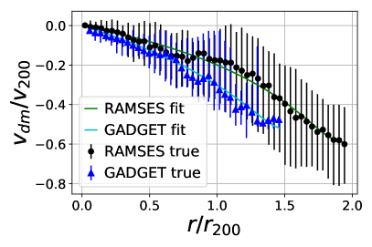
Figure 1: The points represent the median of the normalized mean peculiar radial velocity, $\frac{v_{\rm dm}}{v_{200}}$, for the available clusters at the given radius. The error bars represent $1\sigma$ sample variance between the many simulated clusters. Each cluster has much smaller statistical error-bar, however, the cluster-to-cluster variations lead to this large dispersion. The lines are numerical fits to the infall profiles, using the function described in section 5.

5 Peculiar velocity from numerical simulations

The peculiar velocity of dark matter is shown in figure 1, as a function of radius. The value of $v_{200}$ used to normalize the profiles has been found for each cluster as $\sqrt{\frac{GM_{200}}{r_{200}}}$. The difference between the two simulations arises mainly from the different cluster masses considered, and to a much smaller extend from different cosmological parameters used. For different cosmological models the turn around radius (where the average radial velocity is zero) changes, for instance for a larger cosmological constant the turn around radius is at smaller radii, as can be seen from the spherical collapse model (Pavlidou & Tomaras, 2014). For different cluster masses the detailed infall profile changes significantly (Pivato et al., 2006; Cuesta et al., 2008). Recently Lee & Yepes (2016) tried to quantify this effect, and fitted the peculiar velocities to the form suggested by (Falco et al., 2013A)

$$v_{\rm dm}=-a\,\left(\frac{r}{r_{\rm vir}}\right)^{-b}\,.$$ (11)

They found that $b$ is about $0.26$ for structures of masses $\sim 4\times 10^{13}M_{\odot}$, and increases to $b=0.43$ for masses above $10^{14}M_{\odot}$.

In figure 2 we show the ratio between the DM and the gas infall profiles. From this figure it is clear, that the both AMR and SPH simulations give very similar infall profiles for the gas and the DM. For a given cosmology and cluster mass, it is expected that the gas and DM infall profiles should agree outside the radius where gas cooling becomes important, as discussed in section 3. The similarity of gas and DM infall profiles is expected to break down for smaller structures like galaxies with masses $\sim 10^{12}M_{\odot}$ as shown by (Wetzel & Nagai, 2015). The gas cooling (and star formation and feedback) has very little effect for the large masses considered here, which is seen by the infall profiles essentially agreeing between the two different numerical simulations in the innermost regions.

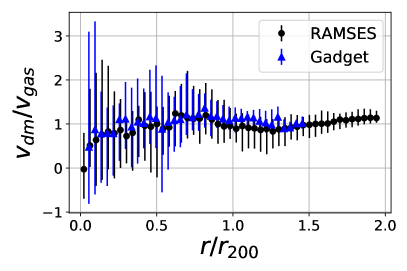
Figure 2: The ratio of the DM to the gas infall profiles, showing that the gas and dark matter have virtually identical infall profiles.

Having found the peculiar velocity, we can now consider the extra mass terms in the generalized hydrostatic equilibrium and Jeans equations.

The two mass excess terms differ only in that $S(r,t)$ depends on the average peculiar radial velocity of dark matter particles, $v_{\rm dm}$, while $\widetilde{S}(r,t)$ depends on the peculiar radial fluid velocity of the gas, $v_{\rm gas}$.

In order to calculate the mass excess terms, $S(r,t)$ and $\widetilde{S}(r,t)$, $\frac{\partial v_{\rm dm}}{\partial t}$ and $\frac{\partial v_{\rm dm}}{\partial r}$ must in principle be determined for each simulated cluster. In Falco et al. (2013A) the authors used 7 different methods to attempt to estimate $\frac{\partial v_{\rm dm}}{\partial t}$. Each of the methods was either based on theoretical calculations or on knowledge of the growth rate of clusters in simulations. However, the results were not entirely conclusive. Since the effect of $\frac{\partial v_{\rm dm}}{\partial t}$ is expected to be very similar for the gas and the DM infall, we will ignore that mass excess term for the present analysis. See appendix A and B in (Falco et al., 2013A) for an extended discussion on this point.

The mass excess therefore becomes simply

$$S(r)\equiv H_{0}v_{\rm dm}+H_{0}r\frac{\partial v_{\rm dm}}{\partial r}+v_{\rm dm}\frac{\partial v_{\rm dm}}{\partial r},$$ (12)

with a similar definition for the ICM mass excess $\widetilde{S}(r)$. Since the time evolution of S has been dropped, and since both the simulations used are evolved to the present epoch, the time dependent Hubble parameter $H(t)$ has been reduced to its current value of $H_{0}$.

We chose to fit the infall profile. In the central part one has $\overline{v_{r}}=0$, giving $v_{\rm dm}=-Hr$, so that the fitting function should be linear as $r\to 0$. At large radii there is almost no braking due to the low density there, and all matter is therefore in free fall towards the cluster center. The peculiar kinetic energy of particles is thus simply the negative value of the gravitational potential, $1/2\,v_{\rm dm}^{2}=-\Phi$, if they are assumed to have fallen in from infinity. The density at this radius is a tiny fraction of its central value, so the mass as a function of radius is very nearly a constant $M(r)\approx M_{total}$. This means that if the background density of the universe is neglected, the potential is the Keplarian potential, $\Phi\approx-\frac{GM_{tot}}{r}$. The peculiar radial velocity should therefore be $v_{\rm dm}\approx-\sqrt{\frac{GM_{tot}}{r}}\propto r^{-1/2}$, and the fitting function should then go as $r^{-1/2}$ in the outer part. The precise shape of this part of the curve is not crucial, as it is almost entirely outside the region that is analyzed.

We use the form

$$\frac{v_{\rm dm}}{v_{200}} = f\Big{(}\frac{r}{r_{200}}\Big{)}$$ (13)

$$= -\alpha\frac{1}{\Big{[}(\frac{r}{r_{200}})^{-b}+C(\frac{r}{r_{200}})^{b/2}\Big{]}^{1/b}-D}\,,$$

where $\alpha$, b, C, and D are positive parameters. This is a slightly modified version of eq. (22) in Falco et al. (2013A). It can be seen that for $r\to 0$ the function approaches a linear shape, $f\to-\alpha\frac{r}{r_{200}}$, while for $r\to\infty$ it goes to $f\to-\frac{\alpha}{C}(\frac{r}{r_{200}})^{-1/2}$, as wished. D determines the shape of the function in the intermediate region where braking occurs. The parameter $\alpha$ can either be chosen to act as a free parameter, or be given the value $\alpha=\frac{Hr_{200}}{v_{200}}$, for which the condition of a static central region will be fulfilled. An example of such a fit to the RAMSES simulated profiles gives parameters $\alpha=0.137\pm 0.0069,b=16.8\pm 24,C=8.9\times 10^{-8}\pm 1.6\times 10^{-6}$ and $D=0.314\pm 0.022$, which in figure 1 is seen to provide an acceptable fit. For the Gadget simulation the fit to $\alpha$ is approximately $25\%$ larger, and the other parameters are witin the error-bars quoted above. The shown fit has a $\chi^{2}$ of 1.11 with respect to the data, meaning that the reduced $\chi^{2}$ is 0.25. The reason why the uncertainties on the parameters b and c are so exceptionally large, is because they are very strongly correlated in the inner part of the clusters, where data is available. If further studies should choose to include the free-falling outer regions of the clusters, then it should be possible to break the degeneracy and better constrain these two parameters. The turn-around is barely visible when considering only radii within two virial radii, which leads the variable $C$ to be consistent with zero. If we fix $C=0$, i.e. having no turn-around in velocity, then the best fit parameters are $\alpha=0.143$ and $D=0.289$ for the RAMSES simulation.

Using this fit, we can calculate the resulting mass excess terms in eqs. (7,10) which is shown in the top panel of Fig. 3. Each of the 3 new terms in the generalized hydrostatic equilibrium and generalized Jeans equations are shown in the lower panel of Fig. 3.

First, we see clearly that inside the virial radius, there is no effect of the combination of Hubble flow and infall. At radii between 1 and 2 virial radii, we see that the radial velocity affects the mass estimates up to $40\%$, both for gas and dark matter.

The mass excess of the dark matter found this way is in good agreement with Falco et al. (2013A), where the mass excess of the galaxy component in simulated clusters was estimated and found to be between 20% and 40% inside 2 $r_{200}$.

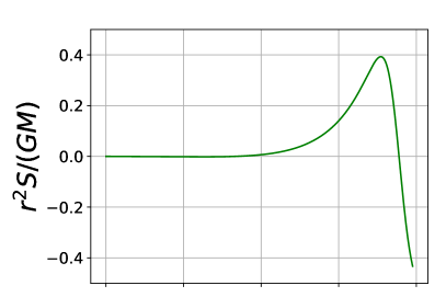
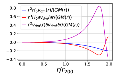
Figure 3: The resulting mass excess divided by the total mass. Upper panel: Inside the virial radius there is no effect of the combination of Hubble flow and infall. Upper panel: At radii between 1 and 2 virial radii the mass estimates is systematically shifted up to $40\%$, both for gas and dark matter. Lower panel: Each of the 3 new terms in the generalized hydrostatic equilibrium.

6 Measuring the magnitude of the velocity infall

This technical section comes with the following warning: the section will conclude that whereas it in principle would be possible to measure a mass excess term coming from the infall profile, in practice it is very difficult. Some readers may therefore prefer to go straight to the concluding section.

It is fair to remind ourselves why we would be interested in measuring the magnitude of the infall velocity profile. The infall velocity is determined mainly by the cluster mass and cosmology, as described in section 5 (for earlier discussions on this point, see e.g. Silk (1974); Regos & Geller (1989); Zu & Weinberg (2013)). For instance the value of the cosmological constant will affect the position of the turn around radius, which is the radius where the infall velocity exactly cancells the Hubble expansion (Pavlidou & Tomaras, 2014). Similarly, various modified gravity models have predictions for the magnitude of the infall velocity, which differs from those of $\Lambda$CDM (Lee & Li, 2016).

The infall velocity leads to a mass excess term, as shown in eq. (6). It is clear from the generalized hydrostatic equilibrium, eq. (LABEL:b5), that if one can simultaneously measure accurately the total mass (for instance from lensing) and gas density and temperature (for instance from either X-ray or SZ), then one can directly get the mass excess term, and hence estimate the mass excess contribution from the velocity infall.

This is, however, rather non-trivial, since a combination of observational techniques always requires a careful control of systematic effects. We will instead here entertain the possibility of using only one method to measure gas parameters, and not include any measure of the total mass. The X-ray method is very well established (Sarazin, 1986), however, it is also clear that the effect of clumping may affect the precision of the mass determination, in particular in the outer regions (see Battaglia et al. (2015) for a recent overview). Only few X-ray observations have today observed to the virial radius (Urban et al., 2014).

The SZ effect, on the other hand, is linear in both temperature and density (Sunyaev & Zeldovich, 1972), which makes it possible to measure the cluster temperature (Pointecouteau et al., 1998; Hansen et al., 2002) without concerns about clumpiness. Future SZ observatories may in principle deproject the spectra to get the full temperature and density profiles (Hansen, 2004).

In principle the full velocity profile may be measured, but for clarity we will here treat it as a one parameter search. This could be the normalization $\alpha$ in eq. (13). We therefore consider the situation where the gas temperature and density have been measured accurately to large radii (e.g. two virial radii) and that $\alpha$ is unknown.

Let us clarify how to measure the magnitude of the infall velocity. Pick a value of $\alpha$. From the generalized hydrostatic equilibrium, eq. (LABEL:b5) one can now calculate everything on the r.h.s. This gives us the total mass, $M_{\rm tot}(r)$. By subtracting the gas mass, we can now derive the dark matter density, which is one of the parameters of the generalized Jeans equation, eq. (LABEL:gje2).

Using numerical simulations, the ratio of the gas temperature and the dark matter “temperature” (i.e. the mean non-translational kinetic energy of dark matter particles) can be parametrized. This is a number which today is believed to be fairly close to unity (Host et al., 2009), and future numerical simulations will determine this ratio much more accurately. Thereby we get $\sigma_{r}^{2}$ in the generalized Jeans equation, eq. (LABEL:gje2). The dark matter velocity anisotropy, $\beta$, is known to follow the density profile of the dark matter (Hansen & Moore, 2006), or alternatively it can be parametrized from numerical simulations (see e.g. Rasia et al. (2006)). The last term is the mass excess term for the dark matter, but as we have found in this paper, it is virtually identical to the one of the gas, so with the assumed value for $\alpha$, it is known. One can therefore derive the total mass from the generalized Jeans equation, eq. (LABEL:gje2).

We thus get the total mass in two different ways, and these can be compared. If they do not agree very well, then we consider a different value for $\alpha$. One loops over values of $\alpha$, and then use some statistical optimization (like $\chi^{2}$).

It is worth repeating where the difference between the two derived total mass profiles appears: if we consider a wrong value for $\alpha$, then the derived mass from eq. (LABEL:b5) is wrong, and hence the derived density profile for the dark matter becomes wrong. This is a rather subtle effect, and very high precision is needed, both in level of equilibration, observation, and the parametrized ratio of gas to dark matter “temperatures”. Most likely this will not be possible in the near future. The differences between numerical techniques (AMR or SPH) still give a too large systematic variation between the ratio of the dark matter and gas temperature. In addition there are other known contributions to non-thermal pressure (see the list of references on this issue in the introduction). In a concrete implementation the measured infall profile is therefore drowned in systematic error-bars. It therefore makes little sense to implement the technique described above until the origin of this difference between numerical simulation techniques has been identified and clarified. The alternative might be to include an independent measurement of the total mass, e.g. from lensing.

We have hereby shown that whereas it in principle would be possible to measure a mass excess term coming from the infall profile, in practice it is very difficult. Furthermore, there will be other effects which also induce a mass excess: When using X-ray temperatures there is the problem of clumpiness, which could induce mass excess of the order $20\%$ near the virial radius (Avestruz et al., 2016; Planelles et al., 2016). This problem could potentially be avoided by using the SZ effect to measure the temperature and density. Furthermore, there could be bulk rotation or turbulence. These effects would be very difficult to remove from the data. And finally, the entire analysis gets even more convoluted (or impossible) when considering that structures usually depart from sphericity, see for instance the discussion in Samsing et al. (2012); Suto et al. (2016); Vega-Ferrero et al. (2016).

7 Conclusion

We compare the infall velocity near galaxy clusters from cosmological simulations, and we find that the gas and dark matter infall profiles are very similar. We derive the relevant gas equation, which is a generalization of the hydrostatic equilibrium equation, and we find that within two virial radii the infall velocity induces a mass excess which is less than $40\%$. Inside the virial radius it is negligible. The similar generalized equation has previously been derived for collisionless DM, and it effectively has an equivalent form. We suggest how future detailed observations in principle may be used to measure this infall profile. However, we also point out that the precision of the needed calibration with numerical simulations is still far too low for this method to be used in practice.

References

- Agertz et al. (2007) Agertz, O., Moore, B., Stadel, J., et al. 2007, MNRAS, 380, 963
- Avestruz et al. (2016) Avestruz, C., Nagai, D., & Lau, E. T. 2016, ApJ, 833, 227
- Battaglia et al. (2015) Battaglia, N., Bond, J. R., Pfrommer, C., & Sievers, J. L. 2015, ApJ, 806, 43
- Biffi et al. (2016) Biffi, V., Borgani, S., Murante, G., et al. 2016, arXiv:1606.02293
- Bonafede et al. (2011) Bonafede, A., Dolag, K., Stasyszyn, F., Murante, G., & Borgani, S. 2011, MNRAS, 418, 2234
- Cuesta et al. (2008) Cuesta, A. J., Prada, F., Klypin, A., & Moles, M. 2008, MNRAS, 389, 385
- Falco et al. (2013A) Falco, M., Mamon, G. A., Wojtak, R., Hansen, S. H., & Gottlöber, S. 2013, MNRAS, 436, 2639
- Falco et al. (2013B) Falco, M., Hansen, S. H., Wojtak, R., & Mamon, G. A. 2013, MNRAS, 431, L6
- Fang et al. (2009) Fang, T., Humphrey, P., & Buote, D. 2009, ApJ, 691, 1648
- Gunn & Gott (1972) Gunn, J. E., & Gott, J. R., III 1972, ApJ, 176, 1
- Gunn (1978) Gunn, J. E. 1978, Saas-Fee Advanced Course 8: Observational Cosmology Advanced Course, 1
- Hansen et al. (2002) Hansen, S. H., Pastor, S., & Semikoz, D. V. 2002, ApJL , 573, L69
- Hansen (2004) Hansen, S. H. 2004, MNRAS, 351, L5
- Hansen & Moore (2006) Hansen, S. H., & Moore, B. 2006, New Astronomy, 11, 333
- Heß & Springel (2012) Heß, S., & Springel, V. 2012, MNRAS, 426, 3112
- Host et al. (2009) Host, O., Hansen, S. H., Piffaretti, R., et al. 2009, ApJ, 690, 358
- Landau & Lifshitz (1959) Landau, L. D., & Lifshitz, E. M. 1959, Course of theoretical physics, Oxford: Pergamon Press
- Lau et al. (2009) Lau, E. T., Kravtsov, A. V., & Nagai, D. 2009, ApJ, 705, 1129
- Lee & Li (2016) Lee, J., & Li, B. 2016, arXiv:1610.07268
- Lee & Yepes (2016) Lee, J., & Yepes, G. 2016, ApJ, 832, 185
- Martizzi et al. (2014) Martizzi, D., Mohammed, I., Teyssier, R.& Moore, B., 2014, MNRAS, 440, 2290
- Munari et al. (2013) Munari, E., Biviano, A., Borgani, S., Murante, G., & Fabjan, D. 2013, MNRAS, 430, 2638
- Pavlidou & Tomaras (2014) Pavlidou, V., & Tomaras, T. N. 2014, JCAP, 9, 020
- Peebles (1976) Peebles, P. J. E. 1976, Apj, 205, 318
- Peebles (1993) Peebles, P. J. E. 1993, Principles of Physical Cosmology by P.J.E. Peebles. Princeton University Press
- Pivato et al. (2006) Pivato, M. C., Padilla, N. D., & Lambas, D. G. 2006, MNRAS, 373, 1409
- Planelles et al. (2014) Planelles, S., Borgani, S., Fabjan, D., et al. 2014, MNRAS, 438, 195
- Planelles et al. (2016) Planelles, S., Fabjan, D., Borgani, S., et al. 2016, arXiv:1612.07260
- Pointecouteau et al. (1998) Pointecouteau, E., Giard, M., & Barret, D. 1998, A&A, 336, 44
- Ragone-Figueroa et al. (2013) Ragone-Figueroa, C., Granato, G. L., Murante, G., Borgani, S., & Cui, W. 2013, MNRAS, 436, 1750
- Rasia et al. (2004) Rasia, E., Tormen, G., & Moscardini, L. 2004, MNRAS, 351, 237
- Rasia et al. (2006) Rasia, E., Ettori, S., Moscardini, L., et al. 2006, MNRAS, 369, 2013
- Rasia et al. (2012) Rasia, E., Meneghetti, M., Martino, R., et al. 2012, New Journal of Physics, 14, 055018
- Regos & Geller (1989) Regos, E., & Geller, M. J. 1989, AJ, 98, 755
- Rines & Diaferio (2006) Rines, K., & Diaferio, A. 2006, AJ, 132, 1275
- Samsing et al. (2012) Samsing, J., Skielboe, A., & Hansen, S. H. 2012, ApJ, 748, 21
- Sarazin (1986) Sarazin, C. L. 1986, Reviews of Modern Physics, 58, 1
- Silk (1974) Silk, J. 1974, ApJ, 193, 525
- Shi et al. (2015) Shi, X., Komatsu, E., Nelson, K., & Nagai, D. 2015, MNRAS, 448, 1020
- Shi et al. (2016) Shi, X., Komatsu, E., Nagai, D., & Lau, E. T. 2016, MNRAS, 455, 2936
- Skielboe et al. (2012) Skielboe, A., Wojtak, R., Pedersen, K., Rozo, E., & Rykoff, E. S. 2012, ApJ, 758, L16
- Springel (2005) Springel, V. 2005, MNRAS, 364, 1105
- Sunyaev & Zeldovich (1972) Sunyaev, R. A., & Zeldovich, Y. B. 1972, Comments on Astrophysics and Space Physics, 4, 173
- Suto et al. (2013) Suto, D., Kawahara, H., Kitayama, T., et al. 2013, ApJ, 767, 79
- Suto et al. (2016) Suto, D., Kitayama, T., Nishimichi, T., Sasaki, S., & Suto, Y. 2016, PASJ, 68, 97
- Svensmark et al. (2015) Svensmark, J., Wojtak, R., & Hansen, S. H. 2015, MNRAS, 448, 1644
- Teyssier (2002) Teyssier, R. 2002, A&A, 385, 337
- Urban et al. (2014) Urban, O., Simionescu, A., Werner, N., et al. 2014, MNRAS, 437, 3939
- Vega-Ferrero et al. (2016) Vega-Ferrero, J., Yepes, G., & Gottlöber, S. 2016, arXiv:1603.02256
- Wetzel & Nagai (2015) Wetzel, A. R., & Nagai, D. 2015, ApJ, 808, 40
- Wojtak et al. (2005) Wojtak, R., Łokas, E. L., Gottlöber, S., & Mamon, G. A. 2005, MNRAS, 361, L1
- Zu & Weinberg (2013) Zu, Y., & Weinberg, D. H. 2013, MNRAS, 431, 3319