Light in Power: A General and Parameter-free Algorithm for Caustic Design

1.   Introduction

The field of non-imaging optics deals with the design of optical components whose goal is to transfer the radiation emitted by a light source onto a prescribed target. This question is at the heart of many applications where one wants to optimize the use of light energy by decreasing light loss or light pollution. Such problems appear in the design of car beams, public lighting, solar ovens and hydroponic agriculture. This problem has also been considered under the name of caustic design, with applications in architecture and interior decoration [?].

In this paper, we consider the problem of designing a wide variety of mirrors and lenses that satisfy different kinds of light energy constraints. To be a little bit more specific, in each problem that we consider, one is given a light source and a desired illumination after reflection or refraction which is called the target. The goal is to design the geometry of a mirror or lens which transports exactly the light emitted by the source onto the target. The design of such optical components can be thought of as an inverse problem, where the forward problem would be the simulation of the target illumination from the description of the light source and the geometry of the mirror or lens.

In practice, the mirror or lens needs to satisfy aesthetic and pragmatic design constraints. In many situations, such as for the construction of car lights, physical molds are built by milling and the mirror or lens is built on this mold. Sometimes the optical component itself is directly milled. This imposes some constraints that can be achieved by imposing convexity or smoothness conditions. The convexity constraint is classical since it allows in particular to mill the component with a tool of arbitrary large radius. Conversely, concavity allows to mill its mold. Also, convex mirrors are easier to chrome-plate, because convex surfaces have no bumps in which the chrome would spuriously concentrate [?].

In this paper, we propose a generic algorithm capable of solving eight different caustic design problems, see Figures LABEL:fig:teaser and 1. Our approach relies on the relation between these problems and optimal transport. The algorithm is fully generic in the sense that it can deal with any of the eight caustic-design problems just by changing a formula, and can handle virtually any ideal light source and target. Our contributions are the following:

• We propose a general framework for eight different optical component design problems (i.e. four non-imaging problems, for which we can produce either concave or convex solutions). These problems amount to solving the same light energy conservation equation (see Sec. 3), which involves prescribing the amount of light reflected or refracted in a finite number of directions.

• We propose a single algorithm with no parameter capable to solve this equation for the eight different problems. We will see that, in order to solve this equation, we need to compute integrals over visibility cells, which can be obtained in all cases by intersecting a 3D Power diagram with a planar of spherical domain. The equation is then solved using a damped Newton algorithm.

• In all of the four non-imaging problems, we can construct either a concave or convex optical component, easing their fabrication. Several components can then be combined to produce a single caustic, providing resilience to small obstacles and providing degrees of freedom to to control the shape of the optical system.

• We show that we can solve near-field problems (when the target is at a finite distance) by iteratively solving far-field problems (when the target is a set of directions) for the eight optical component design problems.

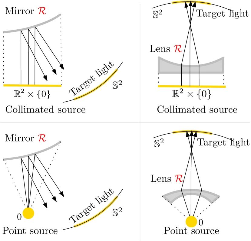
Figure 1: Four inverse problems arising in non-imaging optics. In each case, the goal is to build the surface $\ref{$}ofamirrororalens.Foreachproblem,weprovidetwosolutions(forinstance,convexorconcavesurfaceswhenthelightsourceiscollimated).\textit{Top/Bottom:}Collimatedlightsources/Pointlightsources.\textit{Left/Right:}Mirror/Lensdesign.$

2.   Related work

The field of non-imaging optics has been extensively studied in the last thirty years. We give below an overview of the main approaches to tackle several of the problems of this field. A survey on inverse surface design from light transport behaviour is provided by ? .

Energy minimization methods.

Many different methods to solve inverse problems arising in non-imaging optics rely on variational approaches. When the energies to be minimized are not convex, they can be handled by different kind of iterative methods. One class of methods deals with stochastic optimization. ? propose to represent the optical component (mirror or lens) as a $\mathcal{C}^{2}$ B-spline triangle mesh and to use stochastic optimization to adjust the heights of the vertices so as to minimize a light energy constraint. Note that this approach is very costly, since a forward simulation needs to be done at every step and the number of steps is very high in practice. Furthermore, using this method, lots of artifacts in the final caustic images are present. Stochastic optimization has also been used by ? to design reflective or refractive caustics for collimated light sources. At the center of the method is the Expectation Minimization algorithm initialized with a Capacity Constrained Voronoi Tessellation (CCVT) using a variant of Lloyd’s algorithm [?]. The source is a uniform directional light and is modeled using an array of curved microfacets. The target is represented by a mixture of Gaussian kernel functions. This method cannot accurately handle low intensity regions and artifacts due to the discretization are present. Microfacets were also used by ? to represent the mirror. Due to the sampling procedure, this method cannot correctly handle smooth regions and does not scale well with the size of the target. More recently, ? used microgeometry to design directional screens which provide increased gain and brightness. In their approach, the screen is decomposed into many small patches, each patch reflecting a set of rays toward a prescribed cone of directions. Their problem for each patch is similar to the one we solve for the special case of a directional source and a target at infinity and corresponds to one pillow, see Section LABEL:sec:results. Similarly to us, their approach is based on convex optimization and produce convex patches. They prescribe the areas of the facets, whereas we prescribe their measures. Their numerical approach relies on gradient descent rather than on Newton’s method, and only deals with collimated source and far-field target.

The approaches proposed by ? , ? and ? have in common that they first compute some kind of relationship between the incident rays and their position on the target screen and then use an iterative method to compute the shape of the refractive surface. ? use a continuous parametrization and thus cannot correctly handle totally black and high-contrast regions (boundaries between very dark and very bright areas). ? proposed to use sticks to represent the refractive surface. This allows to reduce production cost, to be more entertaining for the user since a single set of sticks can produce different caustic patterns. The main problem with this approach is the computational complexity since they need to solve a NP-hard assignment problem. The problem of designing lenses for collimated light sources has also been considered by ? . They propose a method to build lenses that can refract complicated and highly contrasted targets. They first use optimal transport on the target space to compute a mapping between the refracted rays of an initial lens and the desired normals, then perform a post-processing step to build a surface whose normals are close to the desired ones.

Monge-Ampère equations

When the source and target lights are modeled by continuous functions, the problem amounts to solving a generalized Monge-Ampère equation, either in the plane for collimated light sources, or on the sphere for point light sources. Let us explain this link more precisely for a collimated light source, assuming that the source rays are collinear to the constant vector $e_{z}=(0,0,1)$ and emitted from a horizontal domain $\Omega\subset\mathbb{R}^{2}\times\{0\}$. We assume that the optical component is smooth and parameterized by a height-field function $\varphi:\Omega\to\mathbb{R}$ and denote by $\mu$ and $\nu$ the source and target measures. At every point $\varphi(x)$ of the optical component, the gradient $\nabla\varphi(x)$ encodes the normal, and we denote by $F(\nabla\varphi(x))\in\mathbb{S}^{2}$ the direction of the ray that is reflected at $(x,\varphi(x))$ using Snell’s law. The conservation of light energy thus reads $\nu(A)=\mu((F\circ\nabla\varphi)^{-1}(A))$ for every set $A$. This is equivalent to having $\tilde{\nu}(B)=\mu((\nabla\varphi)^{-1}(B))$ for every set $B$, where $\tilde{\nu}(B)=\nu(F(B))$. When $F$ and $\nabla\varphi$ are one-to-one (which is the case if the optical component is convex or concave) and $\mu$ and $\tilde{\nu}$ are modeled by continuous functions $f$ and $g$, with the change of variable formula, the light energy conservation becomes equivalent to the following generalized Monge-Ampère equation

$$g(\nabla\varphi(x))\det(D^{2}\varphi(x))=f(x).$$ (1)

Similar equations are obtained for point light sources. The existence and regularity of their solutions, namely of the mirror or lens surfaces, have been extensively studied. When the light source is a point, this problem has been studied for mirrors [?; ?] and lenses [?] and when the light source is collimated one recovers (1) [?]. We refer to the book of ? for an introduction to Monge-Ampère equations.

Optimal transport based methods in non-imaging optics

In fact, the Monge-Ampère equations corresponding to the non-imaging problems considered in this paper can be recast as optimal transport problems. This was first observed by ? and ? for the mirror problem with a point light source. Many algorithms related to optimal transport have been developed to address non-imaging problems. For collimated sources, one could rely on wide-stencils finite difference schemes [?], or on numerical solvers for quadratic semi-discrete optimal transport [?; ?]. For point sources, there exist variants of the Oliker-Prussner algorithm for the mirror problem [?] or the lens problem [?]. Both algorithms have a $\mathrm{O}(N^{4})$ complexity, restricting their use to small discretizations. A quasi-Newton method is proposed by ? for point-source reflector design, handling up to $10^{4}$ Dirac masses.

Finally we note that the approach of ? to build lenses also relies on optimal transport. However, the optimal transport step is used as a heuristic to estimate the normals of the surface, and not to directly construct a solution to the non-imaging problem. A post-processing step is then performed by minimizing a non-convex energy composed of five weighted terms. In contrast, all the results presented in this article use no post-processing.

3.   Light energy conservation

We present in this section several mirror and lens design problems arising in non-imaging optics. In all the problems, one is given a light source (emitted by either a plane or a point) and a desired illumination “at infinity” after reflection or refraction, which is called the target, and the goal is to design the geometry of a mirror or lens which transports the energy emitted by the source onto the target. We do not take into account multiple reflections or refractions. We show that even though the problems we consider are quite different from one another, they share a common structure that corresponds to a so-called generalized Monge-Ampère equation, whose discrete version is given by Equation (2). This section gathers and reformulates in a unified setting results about mirror and lens design for collimated and point light sources. We refer to the work of ? , ? , ? and references therein.

3.1.   Collimated light source

3.1.1 Convex mirror design

In this first problem, the light source is collimated, meaning that it emits parallel rays. The source is encoded by a light intensity function $\rho:\Omega\to\mathbb{R}$ over a 2D domain $\Omega$ contained in the $(xy)$ plane $\mathbb{R}^{2}\times\{0\}\subset\mathbb{R}^{3}$, and that all the rays are parallel and directed towards $e_{z}=(0,0,1)$. For simplicity, we will conflate $\mathbb{R}^{2}$ and $\mathbb{R}^{2}\times\{0\}$. The desired target illumination is “at infinity”, and is described by a set of intensity values $\sigma=(\sigma_{i})_{1\leqslant i\leqslant N}$ supported on a finite set of directions $Y=\{y_{1},\cdots,y_{N}\}$ included in the unit sphere $\mathbb{S}^{2}$. The problem is to find the surface $\ref{$}ofamirrorthatreflectsthesourceintensity$ρ$tothetargetintensity$σ$,seeFigures\leavevmode\nobreak\ \ref{figure:examples-inverseproblems}(topleft)and\ref{figure:collimated_reflector}.\par Sincethenumberofreflecteddirections$Y$isfinite,themirrorsurface$LABEL:$ is composed of a finite number of planar facets as illustrated in Figure 3.1.1. We will construct the mirror $\ref{$}asthegraphofapiecewise-linearconvexfunctionoftheform$x ∈R^2 ↦max_i ⟨x | p_i⟩ - ψ_i$,where$ ⟨⋅ | ⋅⟩ $denotesthedotproduct.Thevectors$p_1,…,p_N ∈R^2$andtheelevations$ψ= (ψ_1,…,ψ_N)∈R^N$havetobedetermined.Tochoose$p_i$,werequirethattheplane$P_i = { (x, ⟨x | p_i⟩) ∣x∈R^2}$reflectsrayswithdirection$e_z$towardsthedirection$y_i∈S^2$.Thedownwardpointingunitnormalto$P_i$isgivenbytheformula$n_i = (p_i,-1)/(∥p_i∥^2 +1) ∈R^3$,andSnell^{\prime}slawofreflectiongivesus$ y_i = e_z - 2 ⟨n_i | e_z⟩ n_i$.Solvingfor$p_i$anddenoting$p_R^2$theorthogonalprojectiononto$R^2 ×{0} $,weget$$p_{i}=-\mathrm{p}_{\mathbb{R}^{2}}(y_{i}-e_{z})/\langle y_{i}-e_{z}|e_{z}\rangle.$$Givenavectorofelevations$ψ:=(ψ_i)_1⩽i ⩽N$,wedefinethevisibilitycell$V_i(ψ)$\mathrm{V}_{i}(\psi)=\{x\in\mathbb{R}^{2}\times\{0\}\mid\leavevmode\nobreak\ \forall j,-\langle x|p_{i}\rangle+\psi_{i}\leqslant-\langle x|p_{j}\rangle+\psi_{j}\}.$$Byconstruction,forevery$i∈{1,…,N}$,anyverticalrayemanatingfromapoint$x ∈V_i(ψ)$touchesthemirrorsurface$LABEL:$ at an altitude $\langle x|p_{i}\rangle-\psi_{i}$, and is thus reflected towards direction $y_{i}$. Consequently, the amount of light reflected towards direction $y_{i}$ equals the integral of $\rho$ over $V_{i}(\psi)$. The Collimated Source Mirror problem (CS/Mirror) then amounts to finding elevations $\psi\in\mathbb{R}^{N}$ such that

$$\forall i\in\{1,\cdots,n\}\quad\int_{\mathrm{V}_{i}(\psi)}\rho(x)\mathrm{d}x=\sigma_{i}.$$ (2)

By construction, a solution to Equation (2) provides a parameterization $\ref{_}\psi$ of a convex mirror that reflects the collimated light source $\rho$ to the discrete target $\sigma$:

$$\ref{_}{\psi}:\ x\in\mathbb{R}^{2}\ \mapsto\ (x,\max_{i}\langle x|p_{i}\rangle-\psi_{i})\in\mathbb{R}^{3},$$

where $\mathbb{R}^{2}\times\{0\}$ and $\mathbb{R}^{2}$ are identified. Notice that since the mirror is a graph over $\mathbb{R}^{2}\times\{0\}$, the vectors $y_{i}$ cannot be upward vertical. In practice we assume that every direction $y_{i}$ belongs to the hemisphere $\mathbb{S}^{2}_{-}:=\{x\in\mathbb{S}^{2},\ \langle x|e_{z}\rangle\leqslant 0\}$. Furthermore, we localize the position of the mirror by considering it only above the domain $X_{\rho}:=\{x\in\mathbb{R}^{2}\times\{0\},\leavevmode\nobreak\ \rho(x)\neq 0\}$.

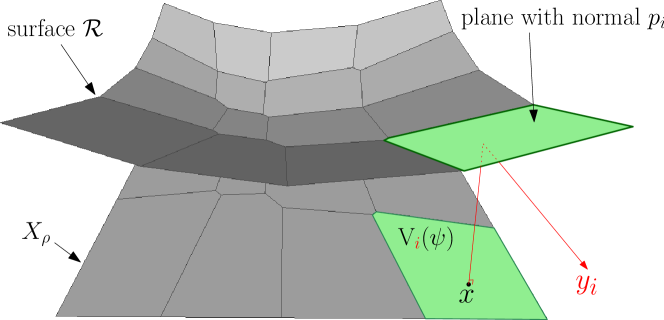
Figure 2: Convex Mirror for a collimated light source (when $N=16$). The mirror surface $\ref{$}isthegraphofaconvexpiecewiseaffinefunction.Thesupport$X_ρ$of$ρ$isdecomposedintovisibilitycells$(V_i(ψ))_1⩽i ⩽N$.Everyverticalrayaboveapoint$x∈X_ρ$belongstoacell$V_i(ψ)$,touchesaplanewithslope$p_i$andisreflectedtothedirection$y_i.

Concave mirror.

The same approach also allows the construction of concave mirrors, using a concave function of the form $x\mapsto\min_{i}\langle x|p_{i}\rangle+\psi_{i}$. This amounts to replacing the visibility cells by

$$\mathrm{V}_{i}(\psi)=\{x\in\mathbb{R}^{2}\times\{0\}\mid\leavevmode\nobreak\ \langle x|p_{i}\rangle+\psi_{i}\leqslant\langle x|p_{j}\rangle+\psi_{j}\leavevmode\nobreak\ \forall j\}.$$

In that case, a solution to Equation (2) provides a parametrization of a concave mirror $\ref{_}{\psi}(x)=(x,\min_{i}\langle x|p_{i}\rangle+\psi_{i})$ that sends the collimated light source $\rho$ to the discrete target $\sigma$.

3.1.2 Convex lens design

In this second design problem, we are interested in designing lenses that refract a given collimated light source intensity $\rho$ to a target intensity $\sigma$, see the top right diagram in Figure 1. We denote by $n_{1}$ the refractive index of the lens, by $n_{2}$ the ambient space refractive index and by $\kappa=n_{1}/n_{2}$ the ratio of the two indices. We assume that the rays emitted by the source are vertical and that the bottom of the lens is flat and orthogonal to the vertical axis. There is no refraction angle when the rays enter the lens, and we only need to build the top part of the lens.

By a simple change of variable, we show that this problem is equivalent to (CS/Mirror). More precisely, for every $y_{i}\in Y$, we now define $p_{i}$ to be the slope of a plane that refracts the vertical ray $e_{z}$ to the direction $y_{i}$. We define $\ref{$}asthegraphofaconvexfunctionoftheform$x↦max_i ⟨x | p_i⟩ - ψ_i$,where$ψ=(ψ_i)_1⩽i ⩽N$isthesetofelevations.{Acalculationsimilartothe(CS/Mirror)casegivesthefollowingexpression:$$p_{i}=-\mathrm{p}_{\mathbb{R}^{2}}(y_{i}-\kappa e_{z})/\langle y_{i}-\kappa e_{z}|e_{z}\rangle.$$Inthatcase,}wedefinethevisibilitycell$V_i(ψ)$tobethesetofpoints$x∈R^2 ×{0} $thatarerefractedtothedirection$y_i$:$$\mathrm{V}_{i}(\psi)=\{x\in\mathbb{R}^{2}\times\{0\}\mid\forall j,\leavevmode\nobreak\ -\langle x|p_{i}\rangle+\psi_{i}\leqslant-\langle x|p_{j}\rangle+\psi_{j}\}.$$The\textit{Collimated Source Lens problem}(CS/Lens)thenamountstofindingweights$(ψ_i)_1⩽i ⩽N$thatsatisfy(\ref{eq:LEC}).Inthatcasethelenssurfaceisparameterizedby$$\ref{_}\psi:\ x\in\mathbb{R}^{2}\ \mapsto\ (x,\max_{i}\langle x|p_{i}\rangle-\psi_{i}).$$Inpractice,wechoosethedirections$y_i$in$S^2_+$andthemirrortobeparameterizedoverthesupport$X_ρ$of$ρ.

Concave lens.

Note that we can also build concave lenses by considering parameterizations with concave functions of the form $x\mapsto\min_{i}\langle x|p_{i}\rangle+\psi_{i}$. Figure 3 illustrates a concave and a convex solution to the same non-imaging optics problem.

Figure 3: Concave and convex lenses for a uniform collimated light source and the same target.

3.2.   Point light source

3.2.1 Concave mirror design.

In this second mirror design problem, all the rays are now emitted from a single point in space, located at the origin, and the light source is described by an intensity function $\rho$ on the unit sphere $\mathbb{S}^{2}$. As in the previous cases, the target is “at infinity” and is described by a set of intensity values $\sigma=(\sigma_{i})_{1\leqslant i\leqslant N}$ supported on the finite set of directions $Y=\{y_{1},\cdots,y_{N}\}\subset\mathbb{S}^{2}$. The problem we consider is to find the surface $\ref{$}ofamirrorthatsendsthelightintensity$ρ$tothelightintensity$σ$(Fig.\leavevmode\nobreak\ \ref{figure:examples-inverseproblems},bottomleft).\par Following\leavevmode\nobreak\ \leavevmode{\immediate{\bf?}},webuildaconcavesurface$LABEL:$ that is composed of pieces of confocal paraboloids. More precisely, we denote by $P(y_{i},\psi_{i})$ the solid (i.e filled) paraboloid whose focal point is at the origin with focal distance $\psi_{i}$ and with direction $y_{i}$. We define the surface $\ref{_}\psi$ as the boundary of the intersection of the solid paraboloids, namely $\ref{_}\psi=\partial\left(\cap_{i}P(y_{i},\psi_{i})\right)$. The visibility cell $\mathrm{V}_{i}(\psi)$ is the set of ray directions $x\in\mathbb{S}^{2}$ emanating from the light source that are reflected in the direction $y_{i}$. Since each paraboloid $\partial P(y_{i},\psi_{i})$ is parameterized over the sphere by $x\mapsto\psi_{i}x/(1-\langle x|y_{i}\rangle)$, one has [?]

$$\mathrm{V}_{i}(\psi)=\left\{x\in\mathbb{S}^{2}\mid\leavevmode\nobreak\ \forall j,\frac{\psi_{i}}{1-\langle x|y_{i}\rangle}\leqslant\frac{\psi_{j}}{1-\langle x|y_{j}\rangle}\right\}.$$

The Point Source Mirror problem (PS/Mirror) then amounts to finding $(\psi_{i})$ that satisfy the light energy conservation equation (2). The mirror surface is then parameterized by

$$\ref{_}\psi:\ x\in\mathbb{S}^{2}\ \mapsto\ \min_{i}\frac{\psi_{i}}{1-\langle x|y_{i}\rangle}\ x.$$

In practice, we assume that the target $Y$ is included in $\mathbb{S}^{2}_{-}$, that the support $X_{\rho}$ of $\rho$ is included $\mathbb{S}^{2}_{+}:=\{x\in\mathbb{S}^{2},\ \langle x|e_{z}\rangle\geqslant 0\}$, and that the mirror is parameterized over $X_{\rho}$.

One can also define the mirror surface as the boundary of the union (instead of the intersection) of a family of solid paraboloids. Then, the visibility cells become

$$\mathrm{V}_{i}(\psi)=\left\{x\in\mathbb{S}^{2}\mid\leavevmode\nobreak\ \forall j,\frac{\psi_{i}}{1-\langle x|y_{i}\rangle}\geqslant\frac{\psi_{j}}{1-\langle x|y_{j}\rangle}\right\}$$

and a solution to Equation (2) provides a parameterization $\ref{_}\psi(x)=x\max_{i}\psi_{i}/(1-\langle x|y_{i}\rangle)$ of the mirror surface. Let us note that in this case the mirror is neither convex nor concave.

3.2.2 Convex lens design.

We now consider the lens design problem for a point light source. As in the collimated setting, we fix the bottom part of the lens. We choose a piece of sphere centered at the source, so that the rays are not deviated. Following  ? , the lens is composed of pieces of ellipsoids of constant eccentricities $\kappa>1$, where $\kappa$ is the ratio of the indices of refraction. Each ellipsoid $\partial E(y_{i},\psi_{i})$ can be parameterized over the sphere by $x\mapsto\psi_{i}x/(1-\kappa\langle x|y_{i}\rangle)$. The visibility cell of $y_{i}$ is then

$$\mathrm{V}_{i}(\psi)=\left\{x\in\mathbb{S}^{2}\mid\leavevmode\nobreak\ \forall j,\frac{\psi_{i}}{1-\kappa\langle x|y_{i}\rangle}\leqslant\frac{\psi_{j}}{1-\kappa\langle x|y_{j}\rangle}\right\}.$$

The Point Source Lens problem (PS/Lens) then amounts to finding weights $(\psi_{i})_{1\leqslant i\leqslant N}$ that satisfy (2). Note that the top surface of the lens is then parameterized by

$$\ref{_}\psi:\ x\in\mathbb{S}^{2}\ \mapsto\ \min_{i}\frac{\psi_{i}}{1-\kappa\langle x|y_{i}\rangle}\ x.$$

In practice, we choose the set of directions $y_{i}$ to belong to $\mathbb{S}^{2}_{+}$ and the lens to be parameterized over the support $X_{\rho}\subset\mathbb{S}^{2}_{+}$ of $\rho$.

One can also choose to define the lens surface as the boundary of the union (instead of the intersection) of a family of solid ellipsoids. In that case, the visibility cells are given by

$$\mathrm{V}_{i}(\psi)=\left\{x\in\mathbb{S}^{2}\mid\leavevmode\nobreak\ \forall j,\frac{\psi_{i}}{1-\kappa\langle x|y_{i}\rangle}\geqslant\frac{\psi_{j}}{1-\kappa\langle x|y_{j}\rangle}\right\}$$

and a solution to Equation (2) provides a parameterization $\ref{_}\psi(x)=x\max_{i}\psi_{i}/(1-\kappa\langle x|y_{i}\rangle)$ of the lens surface. Let us note that in this case the lens is neither convex nor concave.

3.3.   General formulation

Let $X$ be a domain of either the plane $\mathbb{R}^{2}\times\{0\}$ or the unit sphere $\mathbb{S}^{2}$, $\rho:X\to\mathbb{R}$ a probability density and $Y=\{y_{1},\cdots,y_{N}\}\subset\mathbb{S}^{2}$ be a set of $N$ points. We define the function $G:\mathbb{R}^{N}\to\mathbb{R}^{N}$ by

$$G_{i}(\psi)=\int_{\mathrm{V}_{i}(\psi)}\rho(x)\mathrm{d}x$$

where $G(\psi)=(G_{i}(\psi))_{1\leqslant i\leqslant N}$ and $\mathrm{V}_{i}(\psi)\subset X$ is the visibility cell of $y_{i}$, whose definition depends on the non-imaging problem. Using this notation, Equation (2) can be rephrased as finding weights $\psi=(\psi_{i})_{1\leqslant i\leqslant N}$ such that

$$\forall i\in\{1,\cdots,N\},\quad G_{i}(\psi)=\sigma_{i}.$$ (3)

Many other problems arising in non-imaging optics amount to solving equations of this form. For example, the design of a lens that refracts a point light source to a desired near-field target can also be modeled by a Monge-Ampère equation that has the same structure [?]. In this case, the visibility diagram correspond to the radial projection onto the sphere of pieces of confocal ellipsoids with non constant eccentricities and is not associated to an optimal transport problem.

4.   Visibility and Power cells

The main difficulty to evaluate the function $G$ appearing in Equation (3) is to compute the visibility cells $V_{i}(\psi)$ associated to each optical modeling problem. We show in this section that the visibility cells have always the same structure, allowing us to build a generic algorithm in Section 5. We first need to introduce the notion of Power diagram.

Power diagrams.

Let $P\subseteq\mathbb{R}^{3}\times\mathbb{R}$ be a weighted point cloud, i.e. $P=\{(p_{i},\omega_{i})\}_{1\leqslant i\leqslant N}$ with $p_{i}\in\mathbb{R}^{2}$ and $\omega_{i}\in\mathbb{R}$. The Power cell of the $i$th point $p_{i}$ is given by

$$\operatorname{Pow}_{i}(\mathrm{P}):=\{x\in\mathbb{R}^{3}\mid\forall j,\leavevmode\nobreak\ \left\|x-p_{i}\right\|^{2}+\omega_{i}\leqslant\left\|x-p_{j}\right\|^{2}+\omega_{j}\}.$$

Power cells partition $\mathbb{R}^{3}$ into convex polyhedra up to a negligible set. Power diagrams are well-studied objects appearing in computational geometry [?], and can be computed efficiently in dimension $2$ and $3$. When all the weights are equal, one recover the usual Voronoi diagram.

Visibility diagram as a restricted Power diagram.

We now show that in all the non-imaging problems of Section 3, the visibility cells are of the form

$$V_{i}(\psi)=\operatorname{Pow}_{i}(\mathrm{P})\cap X.$$ (4)

For a collimated source, $X$ denotes the plane $\mathbb{R}^{2}\times\{0\}$ and for a point source, $X$ is the unit sphere $\mathbb{S}^{2}$. The expression of the weighted point cloud $\mathrm{P}=\{(p_{i},\omega_{i})\}$ depends on the problem. We refer to Table 1 and the work of ? for formulas in the (PS/Mirror) case, the other ones being obtained in a similar fashion. Let us show the derivation of the formula in the (CS/Mirror) case, where the $i$th visibility cell is given by

$$\mathrm{V}_{i}(\psi) =\{x\in\mathbb{R}^{2}\times\{0\}\mid\leavevmode\nobreak\ \forall j,-\langle x|p_{i}\rangle+\psi_{i}\leqslant-\langle x|p_{j}\rangle+\psi_{j}\}$$

$$=\{x\in\mathbb{R}^{2}\times\{0\}\mid\leavevmode\nobreak\ \forall j,\left\|x-p_{i}\right\|^{2}+\omega_{i}\leqslant\left\|x-p_{j}\right\|^{2}+\omega_{j}\},$$

where $\omega_{i}=2\psi_{i}-\left\|p_{i}\right\|^{2}$. We conclude that the visibility cells for a convex mirror of the (CS/Mirror) problem are indeed given by (4), where the weighted point cloud is given by the first line of Table 1.

Table 1: Formulas for the weighted points used to define the Power cells in Equation (4) for the various problems. In the lens design problem, $\kappa>0$ is the ratio of the indices of refraction, $\kappa>1$ in the (PS/Lens) setting. Ccv means concave and Cvx convex. $\widetilde{\mathrm{Ccv}}$ means that the optical component converges to a concave one when the discretization tends to infinity.

Type	Points	Weights
Cvx (CS/Mirror)	${p_{i}=-\frac{\mathrm{p}_{\mathbb{R}^{2}}(y_{i}-e_{z})}{\langle y_{i}-e_{z}|e_{z}\rangle}}$	$\omega_{i}=2\psi_{i}-\left\|p_{i}\right\|^{2}.$
Ccv (CS/Mirror)	${p_{i}=\frac{\mathrm{p}_{\mathbb{R}^{2}}(y_{i}-e_{z})}{\langle y_{i}-e_{z}|e_{z}\rangle}}$	$\omega_{i}=2\psi_{i}-\left\|p_{i}\right\|^{2}.$
Cvx (PS/Mirror)	$p_{i}=-\frac{y_{i}}{2\ln(\psi_{i})}$	$\omega_{i}=-\frac{1}{\ln(\psi_{i})}-\frac{1}{4\ln(\psi_{i})^{2}}$
$\widetilde{\mathrm{Ccv}}$ (PS/Mirror)	$p_{i}=y_{i}/(2\ln(\psi_{i}))$	$\omega_{i}=\frac{1}{\ln(\psi_{i}))}-\frac{1}{4\ln(\psi_{i})^{2}}$
Cvx (CS/Lens)	$p_{i}=-\frac{\mathrm{p}_{\mathbb{R}^{2}}(y_{i}-\kappa e_{z})}{\langle y_{i}-\kappa e_{z}|e_{z}\rangle}$	$\omega_{i}=2\psi_{i}-\left\|p_{i}\right\|^{2}$
Ccv (CS/Lens)	$p_{i}=\frac{\mathrm{p}_{\mathbb{R}^{2}}(y_{i}-\kappa e_{z})}{\langle y_{i}-\kappa e_{z}|e_{z}\rangle}$	$\omega_{i}=2\psi_{i}-\left\|p_{i}\right\|^{2}$
Cvx (PS/Lens)	$p_{i}=-\kappa\frac{y_{i}}{2\ln(\psi_{i})}$	$\omega_{i}=-\frac{1}{\ln(\psi_{i})}-\frac{\kappa^{2}}{4\ln(\psi_{i})^{2}}$
$\widetilde{\mathrm{Ccv}}$ (PS/Lens)	$p_{i}=\kappa y_{i}/(2\ln(\psi_{i}))$	$\omega_{i}=\frac{1}{\ln(\psi_{i})}-\frac{\kappa^{2}}{4\ln(\psi_{i})^{2}}$

5.   A generic algorithm

For each optical design problem, given a light source intensity function, a target light intensity function and a tolerance, Algorithm 5 outputs a triangulation of a mirror or a lens that satisfies the light energy conservation equation (2).

The main problem is to find weights $\psi$ such that $G(\psi)=\sigma$ (see Equation (3)). This is done using a damped Newton algorithm similar to recent algorithms that have been shown to have a quadratic local convergence rate for optimal transport problems [?] or for Monge-Ampère equations in the plane [?]. A key point of this algorithm is to enforce the Jacobian matrix $\mathrm{D}G(\psi)$ to always be of rank $N-1$. To this purpose, we need to enforce all along the process that

$$\forall i\in\{1,\ldots,N\},\leavevmode\nobreak\ G_{i}(\psi)>0.$$ (5)

Indeed, first note that since $G$ is invariant under the addition of a constant, the kernel of $\mathrm{D}G(\psi)$ always contains the constant vector $(1,\ldots,1)$. Now note that if we have $G_{i}(\psi)=0$, then the corresponding visibility cell $V_{i}(\psi)$ is empty, which implies that $\nabla G_{i}(\psi)=0$ (the gradient being taken with respect to $\psi$). This is because the gradient of $G_{i}$ involves integral on the boundary $\partial V_{i}(\psi)$, as shown for instance by ? in Theorem 1.3. Hence, if $G_{i}(\psi)=0$, then the rank of $\mathrm{D}G(\psi)$ is at most $N-2$ which prevents from using the Damped Newton method. Our method consists of three steps, described in Algorithm 5:

• Initialization (Sec. 5.1): We first discretize the source density into a piecewise affine density and the target one into a finitely supported measure. Then, we construct initial weights $\psi^{0}$ satisfying $\forall i,G_{i}(\psi^{(0)})>0.$

• Damped Newton (Sec 5.2): We construct a sequence $\psi^{k}$ following Algorithm 2 until $\left\|G(\psi^{k})-\sigma\right\|_{\infty}\leqslant\eta$. The main difficulty here is to evaluate $G(\psi^{k})$ and $\mathrm{D}G(\psi^{k})$.

• Surface construction (Sec LABEL:sec:surface-construction): Finally, we convert the solution $\psi^{k}\in\mathbb{R}^{N}$ into a triangulation. Depending on the non-imaging problem, this amounts to approximating an intersection (or union) of half-spaces (or solid paraboloids, or ellipsoids) by a triangulation.

Input

A light source intensity function $\rho_{in}$.

     A target light intensity function $\sigma_{in}$.

     A tolerance $\eta>0$.

A triangulation $\ref{_}T$ of a mirror or lens. Step 1 Initialization (Section 5.1)

$T,\rho\leftarrow$ DISCRETIZATION_SOURCE($\rho_{in})$

$Y,\sigma\leftarrow$ DISCRETIZATION_TARGET($\sigma_{in}$)

$\psi^{0}\leftarrow$ INITIAL_WEIGHTS($Y$)

Solve Equation (3): $G(\psi)=\sigma$ (Section 5.2)

$\psi\leftarrow$ DAMPED_NEWTON($T,\rho,Y,\sigma,\psi^{0},\eta$)

Construct a triangulation $\ref{_}T$ of $\text{<span class="ltx\_ref ltx\_missing\_label ltx\_font\_italic ltx\_ref\_self">LABEL:\$</span>}(Section\text{<span class="ltx\_ref ltx\_missing\_label ltx\_font\_italic ltx\_ref\_self">LABEL:sec:surface-construction</span>})$

LABEL:_T ←SURFACE_CONSTRUCTION($\psi,\ref{_}\psi$)

5.1.   Initialization

Discretization of light intensity functions

Our framework allows to handle any kind of collimated or point light source or target light intensity functions. It can be for example any positive function on the plane or the sphere (depending on the problem) or a greyscale image, which we see as piecewise affine function. We first approach the support of the source density $\rho$ by a triangulation $T$ and assume that the density $\rho:T\to\mathbb{R}^{+}$ is affine on each triangle. We then normalize $\rho$ by dividing it by the total integral $\int_{T}\rho(x)\mathrm{d}x$.

Similarly, the target light intensity function can also be any discrete probability measure. If the user provides an image, one can transform it into a discrete measure of the form $\sigma=\sum_{i}\sigma_{i}\delta_{y_{i}}$ using Lloyd’s algorithm or more simply by taking one Dirac mass per pixel. We do the latter in all experiments. The target measure is also normalized by dividing with the discrete integral $\sum_{i}\sigma_{i}$. We need $\min_{i}\sigma_{i}>0$ for the damped Newton algorithm, but this is not a restriction: if $\sigma_{i}=0$, we simply remove the corresponding Dirac mass $\delta_{y_{i}}$, thus ensuring that no light is sent towards $y_{i}$.

Input

The source $\rho:T\to\mathbb{R}^{+}$ and target $\sigma=\sum_{i}\sigma_{i}\delta_{y_{i}}$; an initial vector $\psi^{0}$ and a tolerance $\eta>0$.

Step 1

Transformation to an Optimal Transport problem

If $X=\mathbb{R}^{2}\times\{0\}$,

then $\widetilde{\psi}^{0}=\psi^{0}$ (and $\widetilde{G}=G$).

If $X=\mathbb{S}^{2}$,

then $\widetilde{\psi}^{0}=(\ln(\psi^{0}_{i}))_{1\leqslant i\leqslant N}$ (and $\widetilde{G}=(G_{i}\circ\exp)_{1\leqslant i\leqslant N}$).

Solve the equation: $\widetilde{G}(\widetilde{\psi})=\sigma$

Initialization:

$\varepsilon_{0}:=\min\left[\min_{i}G_{i}(\psi^{0}),\leavevmode\nobreak\ \min_{i}\sigma_{i}\right]>0$, $k:=0$.

While

$\left\|\widetilde{G}(\widetilde{\psi}^{k})-\sigma\right\|_{\infty}\geqslant\eta$

-

Compute $d_{k}=-\mathrm{D}\widetilde{G}(\widetilde{\psi}^{k})^{+}(\widetilde{G}(\widetilde{\psi}^{k})-\sigma)$

-

Find the smallest $\ell\in\mathbb{N}$ s.t. $\widetilde{\psi}^{k,\ell}:=\widetilde{\psi}^{k}+2^{-\ell}d_{k}$ satisfies

$$\left\{\begin{aligned} &\min_{i}\widetilde{G}_{i}(\widetilde{\psi}^{k,\ell}))\geqslant\varepsilon_{0}\\ &\left\|\widetilde{G}(\psi^{k,\ell})-\sigma\right\|_{\infty}\leqslant(1-2^{-(\ell+1)})\left\|\widetilde{G}(\widetilde{\psi}^{k})-\sigma\right\|_{\infty}\end{aligned}\right.$$

-

Set $\widetilde{\psi}^{k+1}=\widetilde{\psi}^{k}+2^{-\ell}d_{k}$ and $k\leftarrow k+1$.

$\psi:=(\widetilde{\psi}^{k}_{i})_{1\leqslant i\leqslant N}$ if $X=\mathbb{R}^{2}\times\{0\}$ or

       $\psi:=(\exp(\widetilde{\psi}^{k}_{i}))_{1\leqslant i\leqslant N}$ if $X=\mathbb{S}^{2}$.

ALGORITHM 2 Damped Newton method for $G(\psi)=\sigma$

Choice of the initial family of weights $\psi^{0}$.

As mentioned at the beginning of this section, we need to ensure that at each iteration all the visibility cells have non-empty interiors. In particular, we need to choose a set of initial weights $\psi^{0}=(\psi^{0}_{i})_{1\leqslant i\leqslant N}$ such that the initial visibility cells are not empty.

• For the collimated light sources cases (CS/Mirror) and (CS/Lens), we see that if we choose $\psi^{0}_{i}=\left\|p_{i}\right\|^{2}/2$ then $\omega_{i}=0$, where $p_{i}$ is obtained using the formulas of the Section 4. Then, the visibility diagram becomes a Voronoi diagram, hence $p_{i}\in\mathrm{V}_{i}(\psi^{0})$.

• For the Point Source Mirror (PS/Mirror) case, an easy calculation shows that if we choose $\psi^{0}_{i}=1$, then $-y_{i}\in\mathrm{V}_{i}(\psi^{0})$.

• For the Point Source Lens (PS/Lens) case, we can show that if we also choose $\psi^{0}_{i}=1$, then $y_{i}\in\mathrm{V}_{i}(\psi^{0})$.

Note that the previous expressions for $\psi^{0}$ ensure that $G_{i}(\psi^{0})=\rho(V_{i}(\psi^{0}))>0$ only when the support $X_{\rho}$ of the light source is large enough. As an example in the (PS/Mirror) case, if $-y_{i}\notin X_{\rho}$, then we may have $G_{i}(\psi^{0})=0$. To handle this difficulty, we use a linear interpolation between $\rho$ and a constant density supported on a set that contains the $(-y_{i})$’s. This strategy also works for the (CS/Mirror), (PS/Lens) and (CS/Lens) cases.

5.2.   Damped Newton algorithm

When the light source is collimated (i.e. $X=\mathbb{R}^{2}\times\{0\}$), the problem is known to be an optimal transport problem in the plane for the quadratic cost, the function $G$ is the gradient of a concave function, its Jacobian matrix $\mathrm{D}G$ is symmetric and $\mathrm{D}G\leqslant 0$. Moreover, if $G_{i}(\psi)>0$ for all $i$ and if $X_{\rho}$ is connected, then the kernel of $\mathrm{D}G$ is spanned by $\psi=\mathrm{cst}$. This ensures the convergence of the damped Newton algorithm  [?] presented as Algorithm 2, where $A^{+}$ denotes the pseudo-inverse of the matrix $A$. Practically, taking the pseudo-inverse of $\mathrm{D}\widetilde{G}(\widetilde{\psi}^{k})$ guarantees that the mean of the $\widetilde{\psi}^{k}$ remains constant. In practice, we remove a line and a column of the matrix to make it full rank.

When the light source is a point source, we make the change of variable $\widetilde{\psi}={\ln}(\psi)$ and $\widetilde{G}=G\circ\exp$, so that $G(\psi)=\sigma$ if and only if $\widetilde{G}(\tilde{\psi})=\sigma$. This change of variable turns the optical component design problem into an optimal transport problem, ensuring that $\widetilde{G}$ is the gradient of a concave function and that $\mathrm{D}\widetilde{G}$ is symmetric negative [?], thus easily invertible. In the (PS/Mirror) problem with convex mirrors, the damped Newton algorithm is also provably converging [?].

ALGORITHM 1 Mirror / lens construction