Energy-Efficient Resource Allocation for Cache-Assisted Mobile Edge Computing

Abstract

In this paper, we jointly consider communication, caching and computation in a multi-user cache-assisted mobile edge computing (MEC) system, consisting of one base station (BS) of caching and computing capabilities and multiple users with computation-intensive and latency-sensitive applications. We propose a joint caching and offloading mechanism which involves task uploading and executing for tasks with uncached computation results as well as computation result downloading for all tasks at the BS, and efficiently utilizes multi-user diversity and multicasting opportunities. Then, we formulate the average total energy minimization problem subject to the caching and deadline constraints to optimally allocate the storage resource at the BS for caching computation results as well as the uploading and downloading time durations. The problem is a challenging mixed discrete-continuous optimization problem. We show that strong duality holds, and obtain an optimal solution using a dual method. To reduce the computational complexity, we further propose a low-complexity suboptimal solution. Finally, numerical results show that the proposed suboptimal solution outperforms existing comparison schemes.

I Introduction

With drastic development of mobile devices, new applications with advanced features such as augmented reality, mobile online gaming and multimedia transformation, are emerging. These listed applications are both latency-sensitive and computation-intensive, and are beyond the computing capability of common mobile devices. Mobile edge computing (MEC) is one promising technology which provides the computing capability to support these applications at the wireless edge. In an MEC system, a mobile user’s computation task can be uploaded to a base station (BS) and executed at its attached MEC server, which significantly releases the mobile user’s computation burden. However, at the wireless edge, limited communication and computation resources bring big challenges for MEC systems to satisfy massive demands for these applications [1]. Designing energy-efficient MEC systems requires a joint optimization of communication and computation resources among distributed mobile devices and MEC servers. Such optimal resource allocation has been considered for various types of multi-task MEC systems [2, 3, 4, 5, 6]. For instance, [2, 3, 4, 5] study a multi-user MEC system with one BS and one inelastic task for each user, and minimize the energy consumption under a hard deadline constraint for each task. In [6], the authors investigate a multi-user MEC system with one BS and multiple independent elastic tasks for each user, and consider the minimization of the overall system cost. In particular, the offloading scheduling [2, 4, 6] and transmission time (or power) allocation [3, 4, 5, 6] are considered in these optimizations.

One common assumption adopted in [2, 3, 4, 6, 5] is that the computation tasks for different mobiles are different and the computation results cannot be reused, which may not always hold in practice. For instance, in augmented reality subscriptions for better viewing experience in museums, a processed augmented reality output may be simultaneously or asynchronously used by visitors in the same place [1]. Another example is mobile online game where a processed gaming scene may be requested synchronously by a group of players or asynchronously by individual players. In these scenarios where task requests are highly concentrated in the spatial domain and asynchronously or synchronously repeated in the time domain [7, 8], storing computation results closer to users (e.g., at BSs) for future reuse can greatly reduce the computation burden and latency. For example, in [7], the authors propose a resource allocation approach which allows users to share computation results, and minimize the total mobile energy consumption for offloading under the latency and power constraints. However, this paper focuses on only one computation task and does not consider caching computation results for future demands. The authors of [8] propose collaborative multi-bitrate video caching and processing in a multi-user MEC system to minimize the backhaul load, without considering the energy consumption for task executing and computation result downloading. To the best of our knowledge, how to design energy-efficient cache-assisted MEC systems by jointly optimizing communication, caching and computation resources remains unsolved.

In this paper, we jointly consider communication, caching and computation in a multi-user cache-assisted MEC system consisting of one BS of caching and computing capabilities and multiple users with inelastic computation tasks. We specify each task using three parameters, i.e., the size of the task input, workload and size of the computation result. In addition, we consider the popularity and the randomness in task requirements. Based on this task model, we propose a caching and offloading mechanism which involves task uploading and executing for tasks with uncached computation results as well as computation result downloading for all tasks at the BS, and efficiently utilizes multi-user diversity in task uploading and multicasting opportunities in computation result downloading. Then, we formulate the average total energy minimization problem subject to the caching and deadline constraints to optimally allocate the storage resource at the BS as well as the uploading and downloading time durations. The problem is a challenging mixed discrete-continuous optimization problem. We convert its dual problem to a knapsack problem for caching and multiple convex problems for uploading and downloading time allocation, and obtain the dual optimal solution using the subgradient method. We also show that strong duality holds, and obtain an optimal solution of the primal problem based on the dual optimal solution. To reduce the computational complexity, we further propose a low-complexity suboptimal solution. Finally, numerical results show that the proposed suboptimal solution outperforms existing comparison schemes.

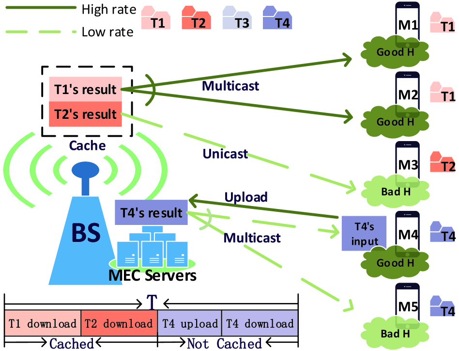
Figure 1: System model. Note that T, M and H are short for task, mobile and channel, respectively. $K=5$, $N=4$ and $|\mathcal{H}|=2$.

II System Model

As illustrated in Fig. 1, we consider a multi-user cache-assisted MEC system with one BS and $K$ single-antenna mobiles, denoted by set $\mathcal{K}\triangleq\{1,2,...,K\}$. The MEC system operates on a frequency band with a bandwidth $B$ (Hz). The BS has powerful caching and computing capabilities at the network edge. Each mobile has a computation-intensive and latency-sensitive computation task which is generated at time 0 and has deadline $T$ (in seconds), and is offloaded to the BS for executing (due to crucial computation and latency requirements). We consider the operation of the MEC system in time interval $[0,T]$. Note that for each user, multiple tasks which are generated at the same time and have the same deadline can be viewed as one super-task whose workload is the sum of the workloads of all its task components. We would like to obtain first-order design insights into caching and computing in cache-assisted MEC. The results obtained in this paper can be extended to study a more general scenario where some tasks can be executed locally and different tasks may have different deadlines.

II-A Task Model and Channel Model

Consider $N$ computation-intensive and latency-sensitive computation tasks, denoted by set $\mathcal{X}\triangleq\{1,\cdots,N\}$. As in [5], each task $n\in\mathcal{X}$ is characterized by three parameters, i.e., the size of the task input $L_{u,n}>0$ (in bits), workload $L_{e,n}>0$ (in number of CPU-cycles), and size of the computation result $L_{d,n}>0$ (in bits). The computation result of each task has to be obtained within $T$ seconds. Note that the three parameters of a computation task are determined by the nature of the task itself, and can be estimated to certain extent based on some prior offline measurements [5]. In addition, the adopted task model properly addresses the limitation in prior work that computation results are assumed to be negligible in size and trivial to download[2, 3].

Different from [5], we focus on the scenario where one task may be required by multiple users, and hence its computation result can be reusable. Examples of these types of applications have been illustrated in Section I. To reflect this characteristic, we model the task popularity. Specifically, mobile $k$ needs to execute a random computation task, denoted by $X_{k}\in\mathcal{X}$. Let $p_{X_{k}}(x_{k})\triangleq\Pr[X_{k}=x_{k}]\geq 0$ denote the probability that the random variable $X_{k}$ takes the value $x_{k}\in\mathcal{X}$. Note that $\sum\limits_{x_{k}\in\mathcal{X}}p_{X_{k}}(x_{k})=1$. Suppose the discrete random variables $X_{k},k\in\mathcal{K}$ are independently distributed, and their probability mass functions (p.m.f.s) $p_{X_{k}}(\cdot)$, $k\in\mathcal{K}$ can be different. Let $\mathbf{X}\triangleq(X_{k})_{k\in\mathcal{K}}\in\mathcal{X}^{K}$ denote the random system task state.

We consider a block fading model for wireless channels. Let $H_{k}\in\mathcal{H}$ denote the random channel state of mobile $k$, representing the power of the channel between mobile $k$ and the BS, where $\mathcal{H}$ denotes the finite channel state space. Assume $H_{k}$ is constant during the $T$ seconds. Let $p_{H_{k}}(h_{k})\triangleq\Pr[H_{k}=h_{k}]\geq 0$ denote the probability that the random variable $H_{k}$ takes the value $h_{k}\in\mathcal{H}$. Note that $\sum\limits_{h_{k}\in\mathcal{H}}p_{H_{k}}(h_{k})=1$. Suppose the discrete random variables $H_{k},k\in\mathcal{K}$ are independently distributed, and their p.m.f.s $p_{H_{k}}(\cdot)$, $k\in\mathcal{K}$ can be different. Let $\mathbf{H}\triangleq(H_{k})_{k\in\mathcal{K}}\in\mathcal{H}^{K}$ denote the random system channel state.

The random system state consists of the random system task state $\mathbf{X}$ and the random system channel state $\mathbf{H}$, denoted by $(\mathbf{X},\mathbf{H})\in\mathcal{X}^{K}\times\mathcal{H}^{K}$. Suppose $\mathbf{X}$ and $\mathbf{H}$ are independent. Thus, the probability that the random system state $(\mathbf{X},\mathbf{H})$ takes the value $(\mathbf{x},\mathbf{h})\in\mathcal{X}^{K}\times\mathcal{H}^{K}$ is given by

$$\Pr[(\mathbf{X},\mathbf{H})=(\mathbf{x},\mathbf{h})]=\prod_{k\in\mathcal{K}}p_{X_{k}}(x_{k})p_{H_{k}}(h_{k})\triangleq p(\mathbf{x},\mathbf{h}),$$ (1)

where $\mathbf{x}\triangleq(x_{k})_{k\in\mathcal{K}}\in\mathcal{X}^{K}$ and $\mathbf{h}\triangleq(h_{k})_{k\in\mathcal{K}}\in\mathcal{H}^{K}$. Each mobile can inform the BS the I.D. of the task it needs to execute, and the BS can easily obtain the channel state of each mobile (e.g., by channel sounding). Thus, we assume that the BS is aware of the system state $(\mathbf{X},\mathbf{H})$.

Let $\mathcal{K}_{n}(\mathbf{X})\triangleq\{k\in\mathcal{K}:X_{k}=n\}$ and $K_{n}(\mathbf{X})\triangleq\sum_{k\in\mathcal{K}}\text{I}\left[X_{k}=n\right]$ denote the set and number of mobiles who need to execute task $n$ at the random system task state $\mathbf{X}$, where $\text{I}[\cdot]$ denotes the indicator function. Note that $K_{n}(\mathbf{X})=|\mathcal{K}_{n}(\mathbf{X})|$. When there exists at least one user requiring to execute task $n$, i.e., $K_{n}(\mathbf{X})\geq 1$, let $H_{u,n}$ and $H_{d,n}$ denote the largest and smallest values among the channel states of all the $K_{n}(\mathbf{X})$ mobiles in $\mathcal{K}_{n}(\mathbf{X})$, respectively, where

$$H_{u,n}\triangleq \max_{k\in\mathcal{K}_{n}(\mathbf{X})}H_{k},\ n\in\mathcal{X},$$ (2)

$$H_{d,n}\triangleq \min_{k\in\mathcal{K}_{n}(\mathbf{X})}H_{k},\ n\in\mathcal{X}.$$ (3)

Note that $H_{u,n}$ and $H_{d,n}$ are determined by $(\mathbf{X},\mathbf{H})$.

II-B Caching and Offloading

First, we consider caching reusable computation results. The BS is equipped with a cache of size $C$ (in bits), and can store some computation results. Let $c_{n}$ denote the caching action for the computation result of task $n$ at the BS, where

$$c_{n}\in\{0,1\},\;n\in\mathcal{X}.$$ (4)

Here, $c_{n}=1$ means that the computation result of task $n$ is cached, and $c_{n}=0$ otherwise. Under the cache size constraint at the BS, we have

$$\sum_{n\in\mathcal{X}}c_{n}L_{d,n}\leq C.$$ (5)

Next, we introduce task offloading. The BS is of computing capability by running a server of a constant CPU-cycle frequency and can execute computation tasks from mobiles. Consider two scenarios in offloading task $n$ to the BS for executing, depending on whether the computation result of task $n$ is stored at the BS or not. If the computation result of task $n$ is not cached at the BS, i.e., $c_{n}=0$, offloading task $n$ to the BS for executing comprises three sequential stages: 1) uploading the input of task $n$ with $L_{u,n}$ bits from the mobile with the best channel $H_{u,n}$ among all the $K_{n}(\mathbf{X})$ mobiles in $\mathcal{K}_{n}(\mathbf{X})$ to the BS; 2) executing task $n$ at the BS (which requires $L_{e,n}$ CPU-cycles); 3) downloading the computation result with $L_{d,n}$ bits from the BS to all the $K_{n}(\mathbf{X})$ mobiles in $\mathcal{K}_{n}(\mathbf{X})$ using multicasting. Note that both the uploading and downloading are over the whole frequency band. Recall that the BS is aware of the system state $(\mathbf{X},\mathbf{H})$. In uploading the input of task $n$, instead of letting each of the $K_{n}(\mathbf{X})$ mobiles in $\mathcal{K}_{n}(\mathbf{X})$ upload separately, the BS selects the mobile with the best channel $H_{u,n}$ to upload. This wisely avoids redundant transmissions and fully makes use of multi-user diversity, leading to energy reduction in uploading. In addition, in downloading the computation result of task $n$, the BS transmits only once at a certain rate so that the mobile with the worst channel $H_{d,n}$ can successfully receive the computation result. Let $t_{u,n}$ denote the downloading time duration for task $n$, where

$$0\leq t_{u,n}\leq T,\ n\in\mathcal{X}.$$ (6)

The BS executing time (in seconds) for task $n$ is $t_{e,n}=L_{e,n}/F_{b}$, where $F_{b}>0$ denotes the fixed CPU-cycle frequency of the BS. As $F_{b}$ is usually large, $t_{e,n}$ is small. In the following, for ease of analysis, we ignore the BS executing time, i.e., assume $t_{e,n}=0$  [4]. Let $t_{d,n}$ denote the downloading time duration for task $n$, where

$$0\leq t_{d,n}\leq T,\ n\in\mathcal{X}.$$ (7)

If the computation result of task $n$ is cached at the BS, i.e., $c_{n}=1$, directly offloading task $n$ to the BS for executing involves only one stage, i.e., downloading the computation result of task $n$ from the BS to all the $K_{n}(\mathbf{X})$ mobiles in $\mathcal{K}_{n}(\mathbf{X})$ using multicasting, with the downloading time duration satisfying (7).

We consider Time Division Multiple Access (TDMA) with Time-Division Duplexing (TDD) operation [5, 3, 2, 4]. Note that when the BS executing time is negligible, the processing order for the offloaded tasks does not matter [5], and the total completion time is the sum of the uploading time durations of the tasks whose computation results are not cached and the downloading time durations of the computation results of all tasks. Thus, under the deadline constraint, we have

$$\sum_{n\in\mathcal{X}}\left((1-c_{n})t_{u,n}+t_{d,n}\right)\leq T.$$ (8)

II-C Energy Consumption

We now introduce the transmission energy consumption model for uploading and downloading. First, consider $c_{n}=0$. Recall that in this case, the mobile with the best channel among all the $K_{n}(\mathbf{X})$ mobiles in $\mathcal{K}_{n}(\mathbf{X})$ uploads task $n$ to the BS. Let $p_{u,n}$ denote the transmission power. Then, the achievable transmission rate (in bit/s) is

$$r_{u,n}=B\log_{2}\left(1+\frac{p_{u,n}H_{u,n}}{n_{0}}\right),$$

where $B$ and $n_{0}$ are the bandwidth and the power of the complex additive white Gaussian noise, respectively. On the other hand, the transmission rate should be fixed as $r_{u,n}=L_{u,n}/t_{u,n}$, since this is the most energy-efficient transmission method for transmitting $L_{u,n}$ bits in $t_{u,n}$ seconds (due to the fact that

$$p_{u,n}=\frac{n_{0}}{H_{u,n}}(2^{r_{u,n}/B}-1)$$

is a convex function of $r_{u,n}$). Define

$$g(x)\triangleq n_{0}\left(2^{\frac{x}{B}}-1\right).$$

Then, we have $p_{u,n}=\frac{1}{H_{u,n}}g\left(\frac{L_{u,n}}{t_{u,n}}\right)$. Thus, at the system state $(\mathbf{X},\mathbf{H})$, the transmission energy consumption for uploading the input of task $n$ to the BS with the uploading time duration $t_{u,n}$ is given by:

$$E_{u,n}(t_{u,n},\mathbf{X},\mathbf{H})\triangleq\begin{cases}\frac{t_{u,n}}{H_{u,n}}g\left(\frac{L_{u,n}}{t_{u,n}}\right),&K_{n}(\mathbf{X})\geq 1\\ 0,&\text{otherwise}\end{cases}\ n\in\mathcal{X},$$ (9)

where $H_{u,n}$ is given by (2). In addition, recall that the BS multicasts the computation result of task $n$ to all the $K_{n}(\mathbf{X})$ mobiles in $\mathcal{K}_{n}(\mathbf{X})$. Thus, similarly, at the system state $(\mathbf{X},\mathbf{H})$, the transmission energy consumption at the BS for multicasting the computation result of task $n$ with the downloading time duration $t_{d,n}$ is given by:

$$E_{d,n}(t_{d,n},\mathbf{X},\mathbf{H})\triangleq\begin{cases}\frac{t_{d,n}}{H_{d,n}}g\left(\frac{L_{d,n}}{t_{d,n}}\right),&K_{n}(\mathbf{X})\geq 1\\ 0,&\text{otherwise}\end{cases}\ n\in\mathcal{X},$$ (10)

where $H_{d,n}$ is given by (3). Then, consider $c_{n}=1$. In this case, the BS directly multicasts the computation result of task $n$ stored at the BS to all the $K_{n}(\mathbf{X})$ mobiles in $\mathcal{K}_{n}(\mathbf{X})$ with the transmission energy $E_{d,n}(t_{d,n},\mathbf{X},\mathbf{H})$ given in (10).

Next, we illustrate the computation energy consumption at the BS. We consider low CPU voltage of the server at the BS. The energy consumption for computation in a single CPU-cycle with frequency $F_{b}$ is $\mu F_{b}^{2}$, where $\mu$ is a constant factor determined by the switched capacitance of the server [3]. Then, the energy consumption for executing task $n$ at the BS is:

$$E_{e,n}(\mathbf{X})\triangleq\begin{cases}\mu L_{e,n}F_{b}^{2},&K_{n}(\mathbf{X})\geq 1\\ 0,&\text{otherwise}\end{cases}\ n\in\mathcal{X}.$$ (11)

Therefore, the energy consumption for task $n$ is given by

$$E_{n}(c_{n},t_{u,n},t_{d,n},\mathbf{X},\mathbf{H})$$

$$\triangleq (1-c_{n})(E_{u,n}(t_{u,n},\mathbf{X},\mathbf{H})+E_{e,n}(\mathbf{X}))+E_{d,n}(t_{d,n},\mathbf{X},\mathbf{H}).$$ (12)

Then, the total energy consumption is given by

$$E(\mathbf{c},\mathbf{t}_{u},\mathbf{t}_{d},\mathbf{X},\mathbf{H})\triangleq\sum_{n\in\mathcal{X}}E_{n}(c_{n},t_{u,n},t_{d,n},\mathbf{X},\mathbf{H}),$$ (13)

where $\mathbf{c}\triangleq(c_{n})_{n\in\mathcal{X}}$, $\mathbf{t}_{u}\triangleq(t_{u,n})_{n\in\mathcal{X}}$ and $\mathbf{t}_{d}\triangleq(t_{d,n})_{n\in\mathcal{X}}$.

III Problem Formulation

Define the feasible joint caching and time allocation policy.

Definition 1 (Feasible Joint Policy)

Consider a joint caching and time allocation policy $(\mathbf{c},\mathbf{T}_{u},\mathbf{T}_{d})$, where the caching design $\mathbf{c}$ does not change with the system state $(\mathbf{X},\mathbf{H})$, and the time allocation design $(\mathbf{T}_{u},\mathbf{T}_{d})$ is a vector mapping (i.e., function) from the system state $(\mathbf{X},\mathbf{H})$ to the time allocation action $(\mathbf{t}_{u},\mathbf{t}_{d})$, i.e., $\mathbf{t}_{u}=\mathbf{T}_{u}(\mathbf{X},\mathbf{H})$ and $\mathbf{t}_{d}=\mathbf{T}_{d}(\mathbf{X},\mathbf{H})$. Here, $\mathbf{T}_{u}\triangleq(T_{u,n})_{n\in\mathcal{X}}$ and $\mathbf{T}_{d}\triangleq(T_{d,n})_{n\in\mathcal{X}}$. We call a policy $(\mathbf{c},\mathbf{T}_{u},\mathbf{T}_{d})$ feasible, if the caching design $\mathbf{c}$ satisfies (4) and (5), and the time allocation action $(\mathbf{t}_{u},\mathbf{t}_{d})$ at each system state $(\mathbf{X},\mathbf{H})$ together with $\mathbf{c}$ satisfies (6), (7) and (8).

Remark 1 (Interpretation of Definition 1)

Caching is in general in a much larger time-scale (e.g., on an hourly or daily basis) and should reflect statistics of the system. In contrast, time allocation is in a much shorter time-scale (e.g., miliseconds) and should exploit instantaneous information of the system. Thus, in Definition 1, we assume that the caching design depends only on the p.m.f.s $p(\mathbf{x},\mathbf{h})$, $(\mathbf{x},\mathbf{h})\in\mathcal{X}^{K}\times\mathcal{H}^{K}$ and does not change with $(\mathbf{X},\mathbf{H})$, while the time allocation design is adaptive to $(\mathbf{X},\mathbf{H})$. In addition, in this paper, we ignore the cost for placing the computation results into the storage at the BS in the initial stage, as the computation results may be useful for much longer time and the initial cost is negligible.

Denote the set of feasible joint policies by $\Pi$. Under a feasible joint policy $(\mathbf{c},\mathbf{T}_{u},\mathbf{T}_{d})\in\Pi$, the average total energy is given by

$$\overline{E}(\mathbf{c},\mathbf{T}_{u},\mathbf{T}_{d})\triangleq\mathbb{E}\left[E(\mathbf{c},\mathbf{T}_{u}(\mathbf{X},\mathbf{H}),\mathbf{T}_{d}(\mathbf{X},\mathbf{H}),\mathbf{X},\mathbf{H})\right],$$ (14)

where the expectation $\mathbb{E}$ is taken over the random system state $(\mathbf{X},\mathbf{H})\in\mathcal{X}^{K}\times\mathcal{H}^{K}$ and $E(\mathbf{c},\mathbf{T}_{u}(\mathbf{X},\mathbf{H}),\mathbf{T}_{d}(\mathbf{X},\mathbf{H}),\mathbf{X},\mathbf{H})$ is given by (13). From (14), we can see that the joint policy $(\mathbf{c},\mathbf{T}_{u},\mathbf{T}_{d})$ significantly affects the average total energy.

In this paper, we would like to obtain the optimal joint feasible policy to minimize the average total energy. Specifically, we have the following optimization problem.

Problem 1 (Average Total Energy Minimization)

$$\overline{E}^{*}\triangleq\min_{(\mathbf{c},\mathbf{T}_{u},\mathbf{T}_{d})\in\Pi} \quad\overline{E}(\mathbf{c},\mathbf{T}_{u},\mathbf{T}_{d})$$

Let $(\mathbf{c}^{*},\mathbf{T}_{u}^{*},\mathbf{T}_{d}^{*})$ and $\overline{E}^{*}$ denote an optimal solution and the optimal value, respectively.

Problem 1 is a very challenging mixed discrete-continuous optimization problem with two types of variables, i.e., the caching design (discrete variables $\mathbf{c}$), and the time allocation design (continuous variables $\mathbf{T}_{u}(\mathbf{X},\mathbf{H}),(\mathbf{X},\mathbf{H})\in\mathcal{X}^{K}\times\mathcal{H}^{K}$ and $\mathbf{T}_{d}(\mathbf{X},\mathbf{H}),(\mathbf{X},\mathbf{H})\in\mathcal{X}^{K}\times\mathcal{H}^{K}$). It can be shown that Problem 1 is NP-hard.

Although Problem 1 is for time interval $[0,T]$, the solution of Problem 1 can be applied to a practical MEC system over a long time during which the task popularity and channel statistics do not change. Specifically, the cached computation results can be used to satisfy task demands after time $T$. In addition, the time allocation design can be used for a group of tasks that are generated at the same time after time $T$ and have the same deadline.

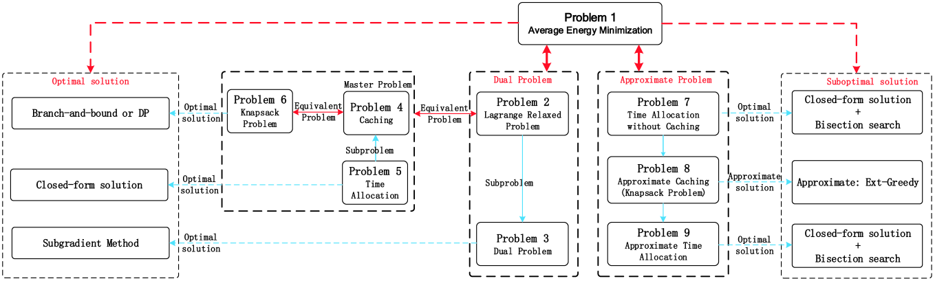
Figure 2: Proposed optimal and suboptimal solutions of Problem 1.

IV Optimal Solution

In this section, we obtain an optimal solution of Problem 1 using a dual method [10], as illustrated in Fig. 2.

IV-A Dual Problem

One challenge in dealing with Problem 1 lies in the fact that it is difficult to handle the deadline constraints for all $(\mathbf{X},\mathbf{H})\in\mathcal{X}^{K}\times\mathcal{H}^{K}$ in (8) (in terms of $T_{u,n}(\mathbf{X},\mathbf{H})$ and $T_{d,n}(\mathbf{X},\mathbf{H})$ instead of $t_{u,n}$ and $t_{d,n}$) where $\mathbf{c}$ and $(\mathbf{T}_{u},\mathbf{T}_{d})$ are coupled. By eliminating the coupling constraints in (8) using nonnegative Lagrangian multipliers $\boldsymbol{\lambda}\triangleq(\lambda(\mathbf{X},\mathbf{H}))_{(\mathbf{X},\mathbf{H})\in\mathcal{X}^{K}\times\mathcal{H}^{K}}\succeq 0$, we form the Lagrangian function $L(\mathbf{c},\mathbf{T}_{u},\mathbf{T}_{d},\boldsymbol{\lambda})$ given in (15).

$$L(\mathbf{c},\mathbf{T}_{u},\mathbf{T}_{d},\boldsymbol{\lambda})=\overline{E}(\mathbf{c},\mathbf{T}_{u},\mathbf{T}_{d})+\sum_{(\mathbf{X},\mathbf{H})\in\mathcal{X}^{K}\times\mathcal{H}^{K}}\lambda(\mathbf{X},\mathbf{H})\left(\sum_{n\in\mathcal{X}}((1-c_{n})T_{u,n}(\mathbf{X},\mathbf{H})+T_{d,n}(\mathbf{X},\mathbf{H}))-T\right)$$ (15)

The dual function $g(\boldsymbol{\lambda})$ can be obtained by solving the following problem.

Problem 2 (Lagrangian Relaxed Problem)

$$g(\boldsymbol{\lambda})\triangleq\min_{\mathbf{c},\mathbf{T}_{u},\mathbf{T}_{d}} \quad L(\mathbf{c},\mathbf{T}_{u},\mathbf{T}_{d},\boldsymbol{\lambda})$$

$$s.t. \quad\eqref{caching},\eqref{eqn:cache-const},\eqref{eqn:time_constraint_1_},\eqref{eqn:time_constraint_2_},$$

where $L(\mathbf{c},\mathbf{T}_{u},\mathbf{T}_{d},\boldsymbol{\lambda})$ is given by (15). Let $(\tilde{\mathbf{c}}^{*}(\boldsymbol{\lambda}),\tilde{\mathbf{T}}^{*}_{u}(\boldsymbol{\lambda}),\tilde{\mathbf{T}}^{*}_{d}(\boldsymbol{\lambda}))$ denote an optimal solution.

The dual problem is given below.

Problem 3 (Dual Problem)

$$g^{*}\triangleq\max_{\boldsymbol{\lambda}} \quad g(\boldsymbol{\lambda})$$

$$s.t. \quad\boldsymbol{\lambda}\succeq 0,$$ (16)

where $g(\boldsymbol{\lambda})$ is given by Problem 2. Let $\boldsymbol{\lambda}^{*}$ and $g^{*}$ denote the optimal dual solution and the optimal dual value, respectively.

By the weak duality theorem[10], $g^{*}\leq\overline{E}^{*}$, where $g^{*}$ is the optimal dual value of the dual problem in Problem 3, and $\overline{E}^{*}$ is the optimal primal value of the primal problem in Problem 1. If $g^{*}=\overline{E}^{*}$ there is no duality gap (i.e., strong duality holds) and if $g^{*}<\overline{E}^{*}$ there is a duality gap. The dual problem in Problem 3 is convex and is more tractable than the primal problem in Problem 1. Note that strong duality does not in general hold for mixed discrete-continuous optimization problems. If we can obtain the optimal dual solution $\boldsymbol{\lambda}^{*}$ and prove that there is no duality gap, an optimal primal solution $(\mathbf{c}^{*},\mathbf{T}_{u}^{*},\mathbf{T}_{d}^{*})$ can be obtained by solving Problem 2 at $\boldsymbol{\lambda}^{*}$, i.e., $(\mathbf{c}^{*},\mathbf{T}_{u}^{*},\mathbf{T}_{d}^{*})=(\tilde{\mathbf{c}}^{*}(\boldsymbol{\lambda}^{*}),\tilde{\mathbf{T}}^{*}_{u}(\boldsymbol{\lambda}^{*}),\tilde{\mathbf{T}}^{*}_{d}(\boldsymbol{\lambda}^{*}))$.

IV-B Optimal Dual Solution

In this part, we solve the dual problem in Problem 3. First, we need to obtain the dual function $g(\boldsymbol{\lambda})$ by solving Problem 2. Note that Problem 2 is also a mixed discrete-continuous optimization problem with two types of variables, i.e., the caching design (discrete variables $\mathbf{c}$), and the time allocation (continuous variables $\mathbf{T}_{u}(\mathbf{X},\mathbf{H}),(\mathbf{X},\mathbf{H})\in\mathcal{X}^{K}\times\mathcal{H}^{K}$ and $\mathbf{T}_{d}(\mathbf{X},\mathbf{H}),(\mathbf{X},\mathbf{H})\in\mathcal{X}^{K}\times\mathcal{H}^{K}$). To facilitate the solution, we equivalently convert Problem 2 into a master problem and multiple subproblems by separating the two types of variables and by noting that $L(\mathbf{c},\mathbf{T}_{u},\mathbf{T}_{d},\boldsymbol{\lambda})$ and $L_{n}(c,t_{u,n},t_{d,n},\mathbf{X},\mathbf{H},\lambda)$ satisfy (17), where $L(\cdot)$ and $L_{n}(\cdot)$ are given by (15) and (18), respectively.

$$L(\mathbf{c},\mathbf{T}_{u},\mathbf{T}_{d},\boldsymbol{\lambda})=\sum_{(\mathbf{X},\mathbf{H})\in\mathcal{X}^{K}\times\mathcal{H}^{K}}\sum_{n\in\mathcal{X}}L_{n}(c_{n},T_{u,n}(\mathbf{X},\mathbf{H}),T_{d,n}(\mathbf{X},\mathbf{H}),\mathbf{X},\mathbf{H},\lambda(\mathbf{X},\mathbf{H}))-T\sum_{(\mathbf{X},\mathbf{H})\in\mathcal{X}^{K}\times\mathcal{H}^{K}}\lambda(\mathbf{X},\mathbf{H})$$ (17)

$$L_{n}(c,t_{u,n},t_{d,n},\mathbf{X},\mathbf{H},\lambda)\triangleq p(\mathbf{X},\mathbf{H})E_{n}(c,t_{u,n},t_{d,n},\mathbf{X},\mathbf{H})+\lambda((1-c)t_{u,n}+t_{d,n})$$ (18)

Specifically, the master problem is for the caching design and is given below.

Problem 4 (Master Problem-Caching)

For all $\boldsymbol{\lambda}\succeq 0$, we have

$$g(\boldsymbol{\lambda})=\min_{\mathbf{c}} \quad\sum_{\mathbf{X}\in\mathcal{X}^{K}}\sum_{\mathbf{H}\in\mathcal{H}^{K}}\sum_{n\in\mathcal{X}}L_{n}^{*}(c_{n},\mathbf{X},\mathbf{H},\lambda(\mathbf{X},\mathbf{H}))$$

$$s.t. \quad~{}\eqref{caching},\eqref{eqn:cache-const},$$

where $L_{n}^{*}(\cdot)$ is given by the following subproblem. Let $\tilde{\mathbf{c}}^{*}(\boldsymbol{\lambda})\triangleq(\tilde{c}_{n}^{*}(\boldsymbol{\lambda}))_{n\in\mathcal{X}}$ denote the optimal solution.

Each subproblem is for the uploading and downloading time allocation for one task at one system state, and is given below.

Problem 5 (Subproblem-Time Allocation)

For all $(\mathbf{X},\mathbf{H})\in\mathcal{X}^{K}\times\mathcal{H}^{K}$, $\lambda$, $n\in\mathcal{X}$ and $c\in\{0,1\}$, we have

$$L_{n}^{*}(c,\mathbf{X},\mathbf{H},\lambda)\triangleq\min_{t_{u,n},t_{d,n}} \quad L_{n}(c,t_{u,n},t_{d,n},\mathbf{X},\mathbf{H},\lambda)$$

$$s.t. \quad\eqref{eqn:time_constraint_1_},\eqref{eqn:time_constraint_2_},$$

where $L_{n}(\cdot)$ is given by (18). Let $\tilde{T}_{u,n}^{*}(c,\mathbf{X},\mathbf{H},\lambda)$ and $\tilde{T}_{d,n}^{*}(c,\mathbf{X},\mathbf{H},\lambda)$ denote the optimal solution.

First, we solve Problem 5. Problem 5 is convex and strong duality holds. Using KKT conditions, we can obtain the optimal solution of Problem 5, which is given below.

Lemma 1 (Optimal Solution of Problem 5)

For all $(\mathbf{X},\mathbf{H})\in\mathcal{X}^{K}\times\mathcal{H}^{K}$, $\lambda$, $n\in\mathcal{X}$ and $c\in\{0,1\}$, the optimal solution of Problem 5 is given by

$$\tilde{T}_{u,n}^{*}(c,\mathbf{X},\mathbf{H},\lambda)=(1-c)f(\mathbf{X},\mathbf{H},L_{u,n},H_{u,n},\lambda),$$ (19)

$$\tilde{T}_{d,n}^{*}(c,\mathbf{X},\mathbf{H},\lambda)=f(\mathbf{X},\mathbf{H},L_{d,n},H_{d,n},\lambda),$$ (20)

where $f(\cdot)$ is given by (21) with $W(\cdot)$ being the Lambert function.

$$f(\mathbf{X},\mathbf{H},x,y,\lambda)\triangleq \min\left\{K_{n}(\mathbf{X}),1\right\}\max\left\{\min\left\{\frac{x\ln 2}{B\left(W\left(\frac{\frac{\lambda y}{p(\mathbf{X},\mathbf{H})}-n_{0}}{n_{0}e}\right)+1\right)},T\right\},0\right\}$$ (21)

$$e_{1,n}(\mathbf{X},\mathbf{H},\lambda)= p(\mathbf{X},\mathbf{H})(E_{u,n}(f(\mathbf{X},\mathbf{H},L_{u,n},H_{u,n},\lambda),\mathbf{X},\mathbf{H})+E_{e,n}(\mathbf{X}))+\lambda f(\mathbf{X},\mathbf{H},L_{u,n},H_{u,n},\lambda)$$ (22)

$$e_{2,n}(\mathbf{X},\mathbf{H},\lambda)= p(\mathbf{X},\mathbf{H})E_{d,n}(f(\mathbf{X},\mathbf{H},L_{d,n},H_{d,n},\lambda),\mathbf{X},\mathbf{H})+\lambda f(\mathbf{X},\mathbf{H},L_{d,n},H_{d,n},\lambda)\$$ (23)

Furthermore, the optimal value of Problem 5 is

$$L_{n}^{*}(c,\mathbf{X},\mathbf{H},\lambda)=(1-c)e_{1,n}(\mathbf{X},\mathbf{H},\lambda)+e_{2,n}(\mathbf{X},\mathbf{H},\lambda),$$

where $e_{1,n}(\cdot)$ and $e_{2,n}(\cdot)$ are given by (22) and (23), respectively.

Next, we solve Problem 4. We introduce the following knapsack problem.

Problem 6 (Knapsack Problem for Caching)

For all $\boldsymbol{\lambda}\succeq 0$, we have

$$\max_{\mathbf{c}} \quad\sum_{n\in\mathcal{X}}c_{n}\sum_{\mathbf{X}\in\mathcal{X}^{K}}\sum_{\mathbf{H}\in\mathcal{H}^{K}}e_{1,n}(\mathbf{X},\mathbf{H},\lambda(\mathbf{X},\mathbf{H}))$$

$$s.t. \quad~{}\eqref{caching},\eqref{eqn:cache-const},$$

where $e_{1,n}(\cdot)$ is given by (22).

By exploring structural properties of Problem 4, we have have the following result.

Lemma 2 (Equivalence between Problem 4 and Problem 6)

An optimal solution of Problem 6 is also optimal for Problem 4.

By Lemma 2, we can obtain $\tilde{\mathbf{c}}^{*}(\boldsymbol{\lambda})$ by solving the knapsack problem in Problem 6 instead of Problem 4. Note that knapsack problem is an NP-hard problem and can be solved optimally using two approaches, i.e., the branch-and-bound method and dynamic programming (DP), with non-polynomial complexity [9]. Substituting $\tilde{\mathbf{c}}^{*}(\boldsymbol{\lambda})$ into the optimal solution of Problem 5 in (19) and (20), we have $\left(\tilde{T}_{u,n}^{*}(\tilde{c}_{n}^{*}(\boldsymbol{\lambda}),\mathbf{X},\mathbf{H},\lambda(\mathbf{X},\mathbf{H})),\tilde{T}_{d,n}^{*}(\tilde{c}_{n}^{*}(\boldsymbol{\lambda}),\mathbf{X},\mathbf{H},\lambda(\mathbf{X},\mathbf{H}))\right)$. With abuse of notation, denote with $(\tilde{T}_{u,n}^{*}(\boldsymbol{\lambda}),\tilde{T}_{d,n}^{*}(\boldsymbol{\lambda}))$ the corresponding mapping. Let $\tilde{\mathbf{T}}_{u}^{*}(\boldsymbol{\lambda})\triangleq(\tilde{T}_{u,n}^{*}(\boldsymbol{\lambda}))_{n\in\mathcal{X}}$ and $\tilde{\mathbf{T}}_{d}^{*}(\boldsymbol{\lambda})\triangleq(\tilde{T}_{d,n}^{*}(\boldsymbol{\lambda}))_{n\in\mathcal{X}}$. Thus, we can obtain an optimal solution of Problem 2, i.e., $(\tilde{\mathbf{c}}^{*}(\boldsymbol{\lambda}),\tilde{\mathbf{T}}_{u}^{*}(\boldsymbol{\lambda}),\tilde{\mathbf{T}}_{d}^{*}(\boldsymbol{\lambda}))$. Furthermore, we can obtain the optimal value of Problem 2, i.e., the dual function $g(\boldsymbol{\lambda})=L(\tilde{\mathbf{c}}^{*}(\boldsymbol{\lambda}),\tilde{\mathbf{T}}^{*}_{u}(\boldsymbol{\lambda}),\tilde{\mathbf{T}}^{*}_{d}(\boldsymbol{\lambda}),\boldsymbol{\lambda})$.

Finally, we solve the dual problem in Problem 3. As there typically exist some Lagrangian multipliers for which Problem 3 has multiple optimal solutions, the dual function $g(\boldsymbol{\lambda})$ is non-differentiable, and gradient methods cannot be applied to solve Problem 3. Here, we consider the subgradient method which uses subgradients as directions of improvement of the distance to the optimum [10]. In particular, for all $(\mathbf{X},\mathbf{H})\in\mathcal{X}^{K}\times\mathcal{H}^{K}$, the subgradient method generates a sequence of dual feasible points according to the following iteration:

$$\lambda_{t+1}(\mathbf{X},\mathbf{H})=\max\left\{\lambda_{t}(\mathbf{X},\mathbf{H})+\alpha_{t}s(\mathbf{X},\mathbf{H},\boldsymbol{\lambda}_{t}),0\right\},$$ (24)

where $s(\mathbf{X},\mathbf{H},\boldsymbol{\lambda}_{t})$ denotes a subgradient of $g(\boldsymbol{\lambda}_{t})$ given by:

$$s(\mathbf{X},\mathbf{H},\boldsymbol{\lambda}_{t})$$

$$= \sum_{n\in\mathcal{X}}\Big{(}(1-\tilde{c}_{n}^{*}(\boldsymbol{\lambda}_{t}))\tilde{T}^{*}_{u,n}(\tilde{c}_{n}^{*}(\boldsymbol{\lambda}_{t}),\mathbf{X},\mathbf{H},\lambda_{t}(\mathbf{X},\mathbf{H}))$$

$$+T^{*}_{d,n}(\tilde{c}_{n}^{*}(\boldsymbol{\lambda}_{t}),\mathbf{X},\mathbf{H},\lambda_{t}(\mathbf{X},\mathbf{H}))\Big{)}-T.$$ (25)

Here, $t$ is the iteration index and $\alpha_{t}$ is the step-size, e.g., $\alpha_{t}=(1+m)/(t+m)$, where $m$ is a fixed nonnegative number. Note that the updates of $\lambda_{t+1}(\mathbf{X},\mathbf{H}),(\mathbf{X},\mathbf{H})\in\mathcal{X}^{K}\times\mathcal{H}^{K}$ are coupled through $\tilde{\mathbf{c}}^{*}(\boldsymbol{\lambda})$. It has been shown in [10] that $\boldsymbol{\lambda}_{t}\to\boldsymbol{\lambda}^{*}$ as $t\to\infty$ for all initial points $\boldsymbol{\lambda}_{0}\succeq 0$. Therefore, using the subgradient method, we can obtain the dual optimal solution $\boldsymbol{\lambda}^{*}$.

IV-C Optimal Primal Solution

Problem 1 is a mixed discrete-continuous optimization problem, for which strong duality does not in general hold. By analyzing structural properties, we show that strong duality holds for Problem 1.

Theorem 1 (Strong Duality)

$g^{*}=\overline{E}^{*}$ holds and $(\mathbf{c}^{*},\mathbf{T}_{u}^{*},\mathbf{T}_{d}^{*})=(\tilde{\mathbf{c}}^{*}(\boldsymbol{\lambda}^{*}),\tilde{\mathbf{T}}_{u}^{*}(\boldsymbol{\lambda}^{*}),\tilde{\mathbf{T}}_{d}^{*}(\boldsymbol{\lambda}^{*}))$.

Theorem 1 indicates that the primal optimal solution $(\mathbf{c}^{*},\mathbf{T}_{u}^{*},\mathbf{T}_{d}^{*})$ can be obtained by the above-mentioned dual method.

In summary, we can obtain an optimal solution $(\mathbf{c}^{*},\mathbf{T}_{u}^{*},\mathbf{T}_{d}^{*})$ by repeating three steps, i.e., solving the caching design problem in Problem 6 (which relies on the optimal solution of the time allocation problem in Problem 5) for given $\boldsymbol{\lambda}_{t}$, solving the time allocation problem in Problem 5 based on the obtained caching design, and updating $\boldsymbol{\lambda}_{t}$ based on the obtained caching design and the time allocation design, until $\boldsymbol{\lambda}_{t}$ converges or stopping criterion is satisfied. The details for obtaining the optimal solution are summarized in Algorithm 1.

Algorithm 1 Optimal Algorithm

1:  Set iteration index $t=0$, and initialize $\boldsymbol{\lambda}_{t}$.

2:  repeat

3:     Obtain $\tilde{\mathbf{c}}^{*}(\boldsymbol{\lambda}_{t})$ by solving Problem 6 using branch-and-bound method or DP.

4:     For all $(\mathbf{X},\mathbf{H})\in\mathcal{X}^{K}\times\mathcal{H}^{K}$ and $n\in\mathcal{X}$, compute $\tilde{T}_{u,n}^{*}(\tilde{c}_{n}^{*}(\boldsymbol{\lambda}),\mathbf{X},\mathbf{H},\lambda(\mathbf{X},\mathbf{H}))$ and $\tilde{T}_{d,n}^{*}(\tilde{c}_{n}^{*}(\boldsymbol{\lambda}),\mathbf{X},\mathbf{H},\lambda(\mathbf{X},\mathbf{H}))$ according to (19) and (20), respectively.

5:     For all $(\mathbf{X},\mathbf{H})\in\mathcal{X}^{K}\times\mathcal{H}^{K}$, compute $\lambda_{t+1}(\mathbf{X},\mathbf{H})$ according to (24), where $s(\mathbf{X},\mathbf{H},\boldsymbol{\lambda}_{t})$ is obtained according to (25).

6:     Set $t=t+1$.

7:  until stopping criterion (e.g., $|s(\mathbf{X},\mathbf{H},\boldsymbol{\lambda}_{t-1})|<\epsilon$, where $\epsilon$ is small and positive) is satisfied.

V Low-Complexity Suboptimal Solution

From (24), we see that $\lambda_{t+1}(\mathbf{X},\mathbf{H})$, $(\mathbf{X},\mathbf{H})\in\mathcal{X}^{K}\times\mathcal{H}^{K}$ all depend on $\boldsymbol{\lambda}_{t}$ via $\tilde{\mathbf{c}}^{*}(\boldsymbol{\lambda}_{t})$. That is, the updates of $\lambda_{t}(\mathbf{X},\mathbf{H})$, $(\mathbf{X},\mathbf{H})\in\mathcal{X}^{K}\times\mathcal{H}^{K}$ are coupled. Thus, $\boldsymbol{\lambda}_{t}$ may converge to $\boldsymbol{\lambda}^{*}$ slowly, leading to high computational complexity for obtaining an optimal solution $(\mathbf{c}^{*},\mathbf{T}_{u}^{*},\mathbf{T}_{d}^{*})$ using the dual method in Section IV, especially when the system state space $\mathcal{X}^{K}\times\mathcal{H}^{K}$ is large. In this section, as illustrated in Fig. 2, we obtain a low-complexity suboptimal solution by carefully handling the coupling among all $(\mathbf{X},\mathbf{H})\in\mathcal{X}^{K}\times\mathcal{H}^{K}$ which results from the coupling between the caching design and the time allocation design. Specifically, instead of joint optimization, we optimize the two designs separately.

Before obtaining a suboptimal caching design, we first ignore storage resource (i.e., by setting $C=0$ and $\mathbf{c}=\mathbf{0}$) and consider Problem 1 with $C=0$ (i.e., minimizing $\overline{E}(\mathbf{0},\mathbf{T}_{u},\mathbf{T}_{d})$ over all feasible $(\mathbf{T}_{u},\mathbf{T}_{d})$ with $(\mathbf{0},\mathbf{T}_{u},\mathbf{T}_{d})\in\Pi$). This problem can be equivalently separated into the following time allocation problems without caching, one for each $(\mathbf{X},\mathbf{H})\in\mathcal{X}^{K}\times\mathcal{H}^{K}$.

Problem 7 (Time Allocation without Caching)

For all $(\mathbf{X},\mathbf{H})\in\mathcal{X}^{K}\times\mathcal{H}^{K}$, we have

$$\min_{\mathbf{t}_{u},\mathbf{t}_{d}} \quad\sum_{n\in\mathcal{X}}E_{n}(0,t_{u,n},t_{d,n},\mathbf{X},\mathbf{H})$$

$$s.t. \quad\eqref{eqn:time_constraint_1_},\eqref{eqn:time_constraint_2_},$$

$$\quad\sum_{n\in\mathcal{X}}\left(t_{u,n}+t_{d,n}\right)\leq T,$$

where $E_{n}(\cdot)$ is given by (12). Let $\left(\mathbf{T}_{u}^{0\dagger}(\mathbf{X},\mathbf{H}),\mathbf{T}_{d}^{0\dagger}(\mathbf{X},\mathbf{H})\right)$ denote the optimal solution, where $\mathbf{T}_{u}^{0\dagger}\triangleq(T_{u,n}^{0\dagger})_{n\in\mathcal{X}}$ and $\mathbf{T}_{d}^{0\dagger}\triangleq(T_{d,n}^{0\dagger})_{n\in\mathcal{X}}$.

Problem 7 is convex and strong duality holds. Similarly, using KKT conditions, we can obtain the optimal solution of Problem 5:

$$T_{u,n}^{0\dagger}(\mathbf{X},\mathbf{H})=f(\mathbf{X},\mathbf{H},L_{u,n},H_{u,n},\lambda^{0\dagger}(\mathbf{X},\mathbf{H})),$$ (26)

$$T_{d,n}^{0\dagger}(\mathbf{X},\mathbf{H})=f(\mathbf{X},\mathbf{H},L_{d,n},H_{d,n},\lambda^{0\dagger}(\mathbf{X},\mathbf{H})),$$ (27)

where $f(\cdot)$ is given by (21) with $W(\cdot)$ being the Lambert function and $\lambda^{0\dagger}(\mathbf{X},\mathbf{H})$ satisfies

$$\sum_{n\in\mathcal{X}}\left(T_{u,n}^{0\dagger}(\mathbf{X},\mathbf{H})+T_{d,n}^{0\dagger}(\mathbf{X},\mathbf{H})\right)=T.$$

As $f(\cdot)$ in (21) is a non-increasing function of $\lambda$, $\lambda^{0\dagger}(\mathbf{X},\mathbf{H})$ can be easily obtained using bisection search.

Then, we take the storage resource into consideration and focus on caching only, i.e, obtaining an optimal caching design which minimizes $\overline{E}(\mathbf{c},\mathbf{T}_{u}^{0\dagger},\mathbf{T}_{d}^{0\dagger})$ subject to (4) and (5). Similarly, this is equivalent to consider the following knapsack problem, which is NP-hard.

Problem 8 (Approximate Knapsack Problem for Caching)

$$\max_{\mathbf{c}} \quad\sum_{n\in\mathcal{X}}c_{n}\sum_{\mathbf{X}\in\mathcal{X}^{K}}\sum_{\mathbf{H}\in\mathcal{H}^{K}}e_{1,n}(\mathbf{X},\mathbf{H},\lambda^{0\dagger}(\mathbf{X},\mathbf{H}))$$

$$s.t. \quad~{}\eqref{caching},\eqref{eqn:cache-const},$$

where $e_{1,n}(\cdot)$ is given by (22).

An approximate solution with $1/2$ optimality guarantee and polynomial complexity can be obtained using the Ext-Greedy algorithm proposed in [9]. Based on the suboptimal solution denoted by $\mathbf{c}^{\dagger}\triangleq(c^{\dagger}_{n})_{n\in\mathcal{X}}$, we then focus on the optimal time allocation design which minimizes $\overline{E}(\mathbf{c}^{\dagger},\mathbf{T}_{u},\mathbf{T}_{d})$ over all feasible $(\mathbf{T}_{u},\mathbf{T}_{d})$ with $(\mathbf{c}^{\dagger},\mathbf{T}_{u},\mathbf{T}_{d})\in\Pi$. Similarly, this problem can be equivalently separated into the following time allocation problems for the given caching design $\mathbf{c}^{\dagger}$, one for each $(\mathbf{X},\mathbf{H})\in\mathcal{X}^{K}\times\mathcal{H}^{K}$.

Problem 9 (Approximate Time Allocation)

Given $\mathbf{c}^{\dagger}$, for all $(\mathbf{X},\mathbf{H})\in\mathcal{X}^{K}\times\mathcal{H}^{K}$, we have

$$\min_{\mathbf{t}_{u},\mathbf{t}_{d}} \quad\sum_{n\in\mathcal{X}}E_{n}(c_{n}^{\dagger},t_{u,n},t_{d,n},\mathbf{X},\mathbf{H})$$

$$s.t. \quad\eqref{eqn:time_constraint_1_},\eqref{eqn:time_constraint_2_},$$

$$\quad\sum_{n\in\mathcal{X}}\left((1-c_{n}^{\dagger})t_{u,n}+t_{d,n}\right)\leq T,$$

where $E_{n}(\cdot)$ is given by (12). Let $\left(\mathbf{T}_{u}^{\dagger}(\mathbf{X},\mathbf{H}),\mathbf{T}_{d}^{\dagger}(\mathbf{X},\mathbf{H})\right)$ denote the optimal solution, where $\mathbf{T}_{u}^{\dagger}\triangleq(T_{u,n}^{\dagger})_{n\in\mathcal{X}}$ and $\mathbf{T}_{d}^{\dagger}\triangleq(T_{d,n}^{\dagger})_{n\in\mathcal{X}}$.

Similarly, we can obtain the optimal solution of Problem 9:

$$T_{u,n}^{\dagger}(\mathbf{X},\mathbf{H})=(1-c_{n}^{\dagger})f(\mathbf{X},\mathbf{H},L_{u,n},H_{u,n},\lambda^{\dagger}(\mathbf{X},\mathbf{H})),$$ (28)

$$T_{d,n}^{\dagger}(\mathbf{X},\mathbf{H})=f(\mathbf{X},\mathbf{H},L_{d,n},H_{d,n},\lambda^{\dagger}(\mathbf{X},\mathbf{H})),$$ (29)

where $f(\cdot)$ is given by (21) with $W(\cdot)$ being the Lambert function and $\lambda^{\dagger}(\mathbf{X},\mathbf{H})$ satisfies

$$\sum_{n\in\mathcal{X}}\left((1-c_{n}^{\dagger})T_{u,n}^{\dagger}(\mathbf{X},\mathbf{H})+T_{d,n}^{\dagger}(\mathbf{X},\mathbf{H})\right)=T.$$

$\lambda^{\dagger}(\mathbf{X},\mathbf{H})$ can be easily obtained using bisection search.

In summary, we can obtain a suboptimal solution $(\mathbf{c}^{\dagger},\mathbf{T}_{u}^{\dagger},\mathbf{T}_{d}^{\dagger})$ by sequentially solving the approximate caching design problem in Problem 8 (which relies on the optimal solution of the time allocation problem without caching in Problem 7) and the approximate time allocation problem in Problem 9. In obtaining the suboptimal solution, for any $(\mathbf{X},\mathbf{H})\in\mathcal{X}^{K}\times\mathcal{H}^{K}$, both $\lambda^{0\dagger}(\mathbf{X},\mathbf{H})$ and $\lambda^{\dagger}(\mathbf{X},\mathbf{H})$ are obtained using efficient bisection search, there is no coupling among $(\mathbf{X},\mathbf{H})\in\mathcal{X}^{K}\times\mathcal{H}^{K}$, and no iterations are required in this process. The details for obtaining the suboptimal solution are summarized in Algorithm 2. It is clear that Algorithm 2 has much lower computational complexity than Algorithm 1.

Algorithm 2 Low-complexity Suboptimal Algorithm

1:  For all $(\mathbf{X},\mathbf{H})\in\mathcal{X}^{K}\times\mathcal{H}^{K}$, compute $\lambda^{0\dagger}(\mathbf{X},\mathbf{H})$ by solving $\sum_{n\in\mathcal{X}}\left(T_{u,n}^{0\dagger}(\mathbf{X},\mathbf{H})+T_{d,n}^{0\dagger}(\mathbf{X},\mathbf{H})\right)=T$ via bisection search;

2:  Compute $\mathbf{c}^{\dagger}$ by solving Problem 8 using the Ext-Greedy algorithm;

3:  For all $(\mathbf{X},\mathbf{H})\in\mathcal{X}^{K}\times\mathcal{H}^{K}$, compute $\lambda^{\dagger}(\mathbf{X},\mathbf{H})$ by solving $\sum_{n\in\mathcal{X}}\left((1-c_{n}^{\dagger})T_{u,n}^{\dagger}(\mathbf{X},\mathbf{H})+T_{d,n}^{\dagger}(\mathbf{X},\mathbf{H})\right)=T$ via bisection search, and for all $n\in\mathcal{X}$, compute $T_{u,n}^{\dagger}(\mathbf{X},\mathbf{H})$ and $T_{d,n}^{\dagger}(\mathbf{X},\mathbf{H})$ according to (28) and (29), respectively.

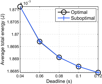
Figure 3: Average total energy versus deadline $T$ at $\gamma=0.8$, $C=5\times 10^{4}$ bits, $K=2,N=3$.

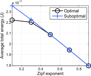
Figure 4: Average total energy versus Zipf exponent $\gamma$ at $T=0.08$ s, $C=5\times 10^{4}$ bits, $K=2,N=3$.

VI Numerical Results

In the numerical experiment, we consider the following settings[3]. Let $B=10$ MHz, $n_{0}=10^{-9}$ W, $\mu=10^{-30}$, $F_{b}=6\times 10^{9}$, $L_{u,n}=n\times 4\times 10^{4}+1\times 10^{4}$ bits, $L_{d,n}=n\times 2\times 10^{4}+1\times 10^{4}$ bits and $L_{e,n}=n\times 4\times 10^{4}+1\times 10^{4}$ CPU-cycles, for all $n\in\mathcal{X}$. Set $\mathcal{H}=\{5\times 10^{-7},1.5\times 10^{-6}\}$ and $p_{H_{k}}(5\times 10^{-7})=0.7015$, $p_{H_{k}}(1.5\times 10^{-6})=0.2581$ for all $k\in\mathcal{K}$. Assume that $X_{k},k\in\mathcal{K}$ follow the same Zipf distribution, i.e., $p_{X_{k}}(n)=\frac{n^{-\gamma}}{\sum_{i\in\mathcal{X}}i^{-\gamma}}$ for all $k\in\mathcal{K}$, where $\gamma$ is the Zipf exponent.

VI-A Comparison Between Optimal and Suboptimal Solutions

In this part, we compare the proposed optimal and suboptimal solutions at small $K$ and $N$ so that the computational complexity for obtaining the optimal solution is manageable. From Fig. 3 and Fig. 4, we can see that the average total energy of the proposed suboptimal solution is very close to that of the optimal solution, demonstrating its applicability at small $K$ and $N$.

VI-B Comparisons with Existing Schemes

In this part, we compare the proposed suboptimal solution with four baseline schemes[3]. All the four baseline schemes view the tasks from different mobiles as different tasks and consider the uploading and downloading of these tasks separately. In addition, Baseline 1 and Baseline 2 make use of the storage resource and adopt the same caching design as the proposed suboptimal solution, while Baseline 3 and Baseline 4 do not consider the caching of computation results. Baseline 1 and Baseline 3 consider equal uploading and downloading time allocation among $K$ mobiles, i.e.,

$$t_{u,n}=t_{d,n}=\begin{cases}\frac{T}{\sum_{i\in\{j\in\mathcal{X}:K_{j}(\mathbf{X})\geq 1\}}(2-c_{i})},&K_{n}(\mathbf{X})\geq 1\\ 0,&\text{otherwise}\end{cases}$$

where $c_{n}=c_{n}^{\dagger}$ for Baseline 1 and $c_{n}=0$ for Baseline 3, for all $n\in\mathcal{X}$. Baseline 2 and Baseline 4 allocate the uploading and downloading time durations for the task of each mobile proportionally to the sizes of its task input and computation result, respectively, i.e.,

$$t_{u,n}=\begin{cases}\frac{L_{u,n}T}{\sum_{i\in\{j\in\mathcal{X}:K_{j}(\mathbf{X})\geq 1\}}((1-c_{i})L_{u,i}+L_{d,i})},&K_{n}(\mathbf{X})\geq 1\\ 0,&\text{otherwise}\end{cases}$$

$$t_{d,n}=\begin{cases}\frac{L_{d,n}T}{\sum_{i\in\{j\in\mathcal{X}:K_{j}(\mathbf{X})\geq 1\}}((1-c_{i})L_{u,i}+L_{d,i})},&K_{n}(\mathbf{X})\geq 1\\ 0,&\text{otherwise}\end{cases}$$

where $c_{n}=c_{n}^{\dagger}$ for Baseline 2 and $c_{n}=0$ for Baseline 4, for all $n\in\mathcal{X}$.

Fig. 5, Fig. 6, Fig. 7 and Fig. 8 illustrate the energy consumption versus different parameters. From Fig. 5, Fig. 6, Fig. 7 and Fig. 8, we can observe that the proposed suboptimal solution outperforms the four baselines, demonstrating the advantage of the proposed suboptimal solution in efficiently utilizing the storage and communication resources. When $\gamma$ increases, the average total energy of each scheme decreases, as the effective task load reduces. When $C$ increases, the average total energies of the proposed suboptimal solution, Baseline 1 and Baseline 2 decrease, due to the energy reduction in task executing. When $K$ or $N$ increases, the average total energy of each scheme increases, due to the increase of the computation load. The performance gains of the proposed suboptimal solution over Baseline 1 and Baseline 2 come from the the fact that the proposed suboptimal solution avoids redundant transmissions in uploading and downloading. Baseline 1 and Baseline 2 outperform Baseline 3 and Baseline 4, respectively, by making use of the storage resource.

VII Conclusion

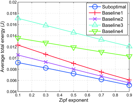
Figure 5: Average total energy versus Zipf exponent $\gamma$ at $C=2.4\times 10^{5}~{}\text{bits},K=4,N=12$, $T=0.08$ s.

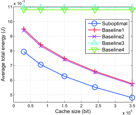
Figure 6: Average total energy versus cache size $C$ at $\gamma=0.8,K=4,N=12$, $T=0.08$ s.

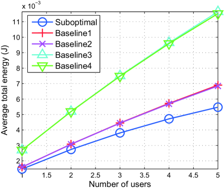
Figure 7: Average total energy versus number of users $K$ at $\gamma=0.8,C=1.5\times 10^{5}~{}\text{bits},N=9$, $T=0.08$ s.

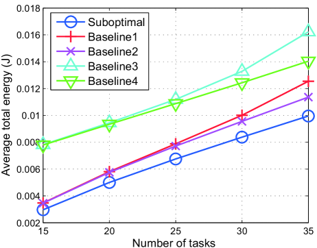
Figure 8: Average total energy versus number of tasks $N$ at $\gamma=0.8,C=3.5\times 10^{5}~{}\text{bits},K=3$, $T=0.08$ s.

In this paper, we consider the average total energy minimization problem subject to the caching and deadline constraints to optimally allocate the storage resource at the BS for caching computation results as well as the uploading and downloading time durations in a multi-user cache-assisted MEC system. The problem is a challenging mixed discrete-continuous optimization problem. We show that strong duality holds, and obtain an optimal solution using a dual method. We further propose a low-complexity suboptimal solution. Finally, numerical results show that the proposed suboptimal solution outperforms existing comparison schemes and reveal the advantage in efficiently utilizing storage and communication resources. This paper provides key insights for designing energy-efficient MEC systems by jointly utilizing communication, caching and computation.

References

• [1] Y. Mao, C. You, J. Zhang, K. Huang, and K. B. Letaief, “Mobile edge computing: Survey and research outlook,” arXiv preprint arXiv:1701.01090, 2017.
• [2] Y. Mao, J. Zhang, and K. B. Letaief, “Dynamic computation offloading for mobile-edge computing with energy harvesting devices,” IEEE J. Sel. Areas Commun., vol. 34, no. 12, pp. 3590–3605, 2016.
• [3] C. You, K. Huang, H. Chae, and B.-H. Kim, “Energy-efficient resource allocation for mobile-edge computation offloading,” IEEE Trans. Wireless Commun., vol. 16, no. 3, pp. 1397–1411, 2017.
• [4] F. Wang, J. Xu, X. Wang, and S. Cui, “Joint offloading and computing optimization in wireless powered mobile-edge computing systems,” arXiv preprint arXiv:1702.00606, 2017.
• [5] J. Guo, Z. Song, Y. Cui, Z. Liu, and Y. Ji, “Energy-efficient resource allocation for multi-user mobile edge computing,” in Proc. IEEE GLOBECOM, 2017, pp. 1–7.
• [6] M.-H. Chen, B. Liang, and M. Dong, “Joint offloading decision and resource allocation for multi-user multi-task mobile cloud,” in Proc. IEEE ICC, 2016, pp. 1–6.
• [7] A. Al-Shuwaili and O. Simeone, “Optimal resource allocation for mobile edge computing-based augmented reality applications,” arXiv preprint arXiv:1611.09243, 2016.
• [8] T. X. Tran, P. Pandey, A. Hajisami, and D. Pompili, “Collaborative multi-bitrate video caching and processing in mobile-edge computing networks,” in Proc. IEEE WONS, 2017, pp. 165–172.
• [9] H. Kellerer, U. Pferschy, and D. Pisinger, Knapsack Problem.   Springer, 2004.
• [10] D. P. Bertsekas, Nonlinear Programming, 2nd ed.   Belmont, MA: Athena Scientific, 1999.