Efficient Compression Technique for Sparse Sets

Abstract.

Recent technological advancements have led to the generation of huge amounts of data over the web, such as text, image, audio and video. Needless to say, most of this data is high dimensional and sparse, consider, for instance, the bag-of-words representation used for representing text. Often, an efficient search for similar data points needs to be performed in many applications like clustering, nearest neighbour search, ranking and indexing. Even though there have been significant increases in computational power, a simple brute-force similarity-search on such datasets is inefficient and at times impossible. Thus, it is desirable to get a compressed representation which preserves the similarity between data points. In this work, we consider the data points as sets and use Jaccard similarity as the similarity measure. Compression techniques are generally evaluated on the following parameters –1) Randomness required for compression, 2) Time required for compression, 3) Dimension of the data after compression, and 4) Space required to store the compressed data. Ideally, the compressed representation of the data should be such, that the similarity between each pair of data points is preserved, while keeping the time and the randomness required for compression as low as possible.

Recently, Pratap and Kulkarni (KulkarniP16, ), suggested a compression technique for compressing high dimensional, sparse, binary data while preserving the Inner product and Hamming distance between each pair of data points. In this work, we show that their compression technique also works well for Jaccard similarity. We present a theoretical proof of the same and complement it with rigorous experimentations on synthetic as well as real-world datasets. We also compare our results with the state-of-the-art ”min-wise independent permutation”, and show that our compression algorithm achieves almost equal accuracy while significantly reducing the compression time and the randomness. Moreover, after compression our compressed representation is in binary form as opposed to integer in case of min-wise permutation, which leads to a significant reduction in search-time on the compressed data.

1. Introduction

We are at the dawn of a new age. An age in which the availability of raw computational power and massive data sets gives machines the ability to learn, leading to the first practical applications of Artificial Intelligence. The human race has generated more amount of data in the last $2$ years than in the last couple of decades, and it seems like just the beginning. As we can see, practically everything we use on a daily basis generates enormous amounts of data and in order to build smarter, more personalised products, it is required to analyse these datasets and draw logical conclusions from it. Therefore, performing computations on big data is inevitable, and efficient algorithms that are able to deal with large amounts of data, are the need of the day.

We would like to emphasize that most of these datasets are high dimensional and sparse – the number of possible attributes in the dataset are large however only a small number of them are present in most of the data points. For example: micro-blogging site Twitter can have each tweet of maximum $140$ characters. If we consider only English tweets, considering the vocabulary size is of $171,476$ words, each tweet can be represented as a sparse binary vector in $171,476$ dimension, where $1$ indicates that a word is present, $0$ otherwise. Also, large variety of short and irregular forms in tweets add further sparseness. Sparsity is also quite common in web documents, text, audio, video data as well.

Therefore, it is desirable to investigate the compression techniques that can compress the dimension of the data while preserving the similarity between data objects. In this work, we focus on sparse, binary data, which can also be considered as sets, and the underlying similarity measure as Jaccard similarity. Given two sets $A$ and $B$ the Jaccard similarity between them is denoted as $\mathrm{JS}(A,B)$ and is defined as $\mathrm{JS}(A,B)={|A\cap B|}/{|A\cup B|}$. Jaccard Similarity is popularly used to determine whether two documents are similar. (setcontainment, ) showed that this problem can be reduced to set intersection problem via shingling . For example: two documents $A$ and $B$ first get converted into two shingles $S_{A}$ and $S_{B}$, then similarity between these two documents is defined as $\mathrm{JS}(A,B)=|S_{A}\cap S_{B}|/|S_{A}\cup S_{B}|$. Experiments validate that high Jaccard similarity implies that two documents are similar.

Broder et al. (Broder00, ; BroderCFM98, ) suggested a technique to compress a collection of sets while preserving the Jaccard similarity between every pair of sets. For a set $\mathrm{U}$ of binary vectors $\{\mathbf{u_{i}}\}_{i=1}^{n}\subseteq\{0,1\}^{d}$, their technique includes taking a random permutation of $\{1,2,\ldots,d\}$ and assigning a value to each set which maps to minimum under that permutation.

Definition 1.1 (Minhash (Broder00, ; BroderCFM98, )).

Let $\pi$ be a permutations over $\{1,\ldots,d\}$, then for a set $\mathbf{u}\subseteq\{1,\ldots d\}$ $h_{\pi}(\mathbf{u})=\arg\min_{i}\pi(i)$ for $i\in\mathbf{u}$. Then,

$$\Pr[h_{\pi}(\mathbf{u})=h_{\pi}(\mathbf{v})]=\frac{|\mathbf{u}\cap\mathbf{v}|}{|\mathbf{u}\cup\mathbf{v}|}.$$

Note 1.2 (Representing sets as binary vectors).

Throughout this paper, for convenience of notation we represent sets as binary vectors. Let the cardinality of the universal set is $d$, then each set which is a subset of the universal set is represented as a binary vector in $d$-dimension. We mark $1$ at position where the corresponding element from universal set is present, and $0$ otherwise. We illustrate this with an example: let the universal set is $\mathcal{U}=\{1,2,3,4,5\}$, then we represent the set $\{1,2\}$ as $11000$, and the set $\{1,5\}$ as $100001$.

1.1. Revisiting Compression Scheme of (KulkarniP16, )

Recently, Pratap and Kulkarni (KulkarniP16, ) suggested a compression scheme for binary data that compress the data while preserving both Hamming distance and Inner product. A major advantage of their scheme is that the compression-length depends only on the sparsity of the data and is independent of the dimension of data. In the following we briefly discuss their compression scheme:

Consider a set of $n$ binary vectors in $d$-dimensional space, then, given a binary vector $\textbf{u}\in\{0,1\}^{d}$, their scheme compress it into a $\mathrm{N}$-dimensional binary vector (say) $\mathbf{u^{\prime}}\in\{0,1\}^{\mathrm{N}}$ as follows, where $\mathrm{N}$ to be specified later. It randomly assign each bit position (say) $\{i\}_{i=1}^{d}$ of the original data to an integer $\{j\}_{j=1}^{\mathrm{N}}$. Further, to compute the $j$-th bit of the compressed vector $\mathbf{u^{\prime}}$ we check which bits positions have been mapped to $j$, and compute the parity of bits located at those positions, and assign it to the $j$-th bit position. Figure 1 illustrate this with an example, and the definition below state is more formally. In continuation of their analogy we call it as $\mathrm{BCS}.$

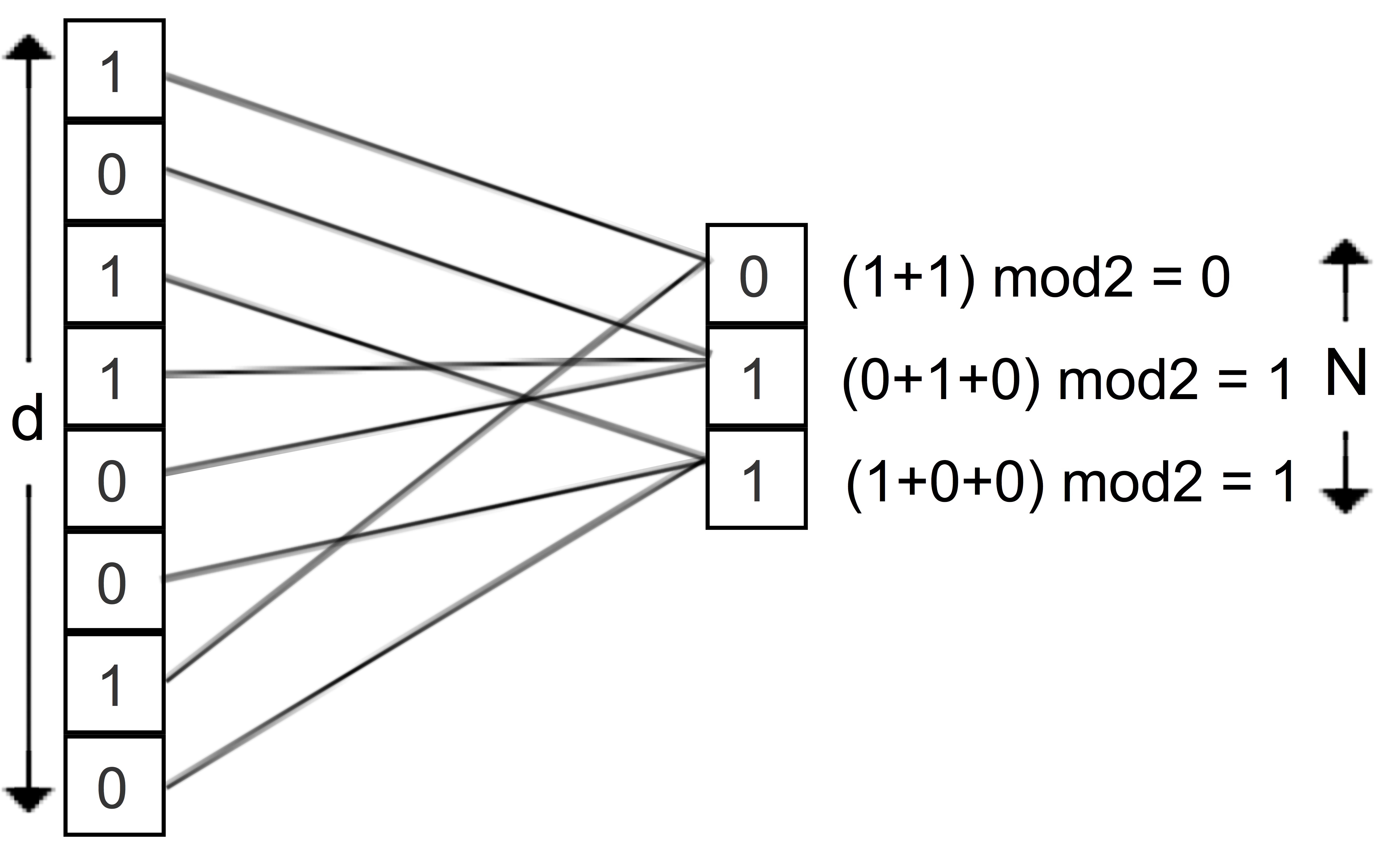
Figure 1. Binary Compression Scheme ($\mathrm{BCS}$) of (KulkarniP16, )

Definition 1.3 (Binary Compression Scheme – $\mathrm{BCS}$ (Definition $3.1$ of (KulkarniP16, )) ).

Let $\mathrm{N}$ be the number of buckets (compression length), for $i=1$ to $d$, we randomly assign the $i$-th position to a bucket number $b(i)$ $\in\{1,\ldots\mathrm{N}\}$. Then a vector $\mathbf{u}\in\{0,1\}^{d}$, compressed into a vector $\mathbf{u}^{\prime}\in\{0,1\}^{\mathrm{N}}$ as follows:

$$\mathbf{u}^{\prime}[j]=\sum_{i:b(i)=j}\mathbf{u}[i]\pmod{2}.$$

1.2. Our Result

Using the above mentioned compression scheme, we are able to prove the following compression guarantee for Jaccard similarity.

Theorem 1.4.

Consider a set $\mathrm{U}$ of binary vectors $\{\mathbf{u_{i}}\}_{i=1}^{n}\subseteq\{0,1\}^{d}$ with maximum number of $1$ in any vector is at most $\mathrm{\psi}$, a positive integer $r$, $\epsilon\in(0,1)$, and $\varepsilon\geq\max\{\epsilon,2\epsilon/1-\epsilon\}$. We set $\mathrm{N}=O({\mathrm{\psi}}^{2}\log^{2}n)$, and compress them into a set $\mathrm{U^{\prime}}$ of binary vectors $\{\mathbf{u_{i}^{\prime}}\}_{i=1}^{n}\subseteq\{0,1\}^{\mathrm{N}}$ via $\mathrm{BCS}$. Then for all $\mathbf{u_{i}},\mathbf{u_{j}}\in\mathrm{U}$ the following holds with probability at least $1-{2}/{n}$,

$$(1-\varepsilon)\mathrm{JS}(\mathbf{u_{i}},\mathbf{u_{j}})\leq\mathrm{JS}({\mathbf{u_{i}}}^{\prime},{\mathbf{u_{j}}}^{\prime})\leq(1+\varepsilon)\mathrm{JS}(\mathbf{u_{i}},\mathbf{u_{j}}).$$

Remark 1.5.

A major benefit (as also mentioned in (KulkarniP16, )) of $\mathrm{BCS}$ is that it also works well in the streaming setting. The only prerequisite is an upper bound on the sparsity $\mathrm{\psi}$ as well as on the number of data points, which requires to give a bound on the compression length $\mathrm{N}$.

Parameters for evaluating a compression scheme

The quality of a compression algorithm can be evaluated on the following parameters.

• Randomness is the number of random bits required for compression.

• Compression time is the time required for compression.

• Compression length is the dimension of data after compression.

• The amount of space required to store the compressed matrix.

Ideally the compression length and the compression time should be as small as possible while keeping the accuracy as high as possible.

1.3. Comparison between $\mathrm{BCS}$ and minhash

We evaluate the quality of our compression scheme with minhash on the parameters stated earlier.

Randomness

One of the major advantages of BCS is the reduction in the number of random bits required for compression. We quantify it below.

Lemma 1.6.

Let a set of $n$ $d$ dimensional binary vectors, which get compressed into a set of $n$ vectors in $\mathrm{N}$ dimension via minhash and $\mathrm{BCS}$, respectively. Then, the amount of random bits required for $\mathrm{BCS}$ and minhash are $O(d\log\mathrm{N})$ and $O(\mathrm{N}d\log d)$, respectively.

Proof.

For $\mathrm{BCS}$, it is required to map each bit position from $d$-dimension to $\mathrm{N}$-dimension. One bit assignment requires $O(\log\mathrm{N})$ amount of randomness as it needs to generate a number between $1$ to $\mathrm{N}$ which require $O(\log\mathrm{N})$ bits. Thus, for each bit position in $d$-dimension, the mapping requires $O(d\log\mathrm{N})$ amount of randomness. On the other side, minhash requires creating $\mathrm{N}$ permutations in $d$-dimension. One permutation in $d$ dimension requires generating $d$ random numbers each within $1$ and $d$. Generating a number between $1$ and $d$ requires $O(\log d)$ random bits, and generating $d$ such numbers require $O(d\log d)$ random bits. Thus, generating $\mathrm{N}$ such random permutations requires $O(\mathrm{N}d\log d)$ random bits.

∎

Compression time

$\mathrm{BCS}$ is significantly faster than Minhash algorithm in terms of compression time. This is because, generation of random bits requires a considerable amount of time. Thus, reduction in compression time is proportional to the reduction in the amount of randomness required for compression. Also, for compression length $\mathrm{N}$, Minhash scans the vector $\mathrm{N}$ times - once for each permutation, while $\mathrm{BCS}$ just requires a single scan.

Space required for compressed data:

Minhash compression generates an integer matrix as opposed to the binary matrix generated by $\mathrm{BCS}$. Therefore, the space required to store the compressed data of $\mathrm{BCS}$ is $O(\log d)$ times less as compared to minhash.

Search time

Binary form of our compressed data leads to a significantly faster search as efficient bitwise operations can be used.

In Section 3, we numerically quantify the advantages of our compression on the later three parameters via experimentations on synthetic and real-world datasets.

Li et. al. (Libit, ) presented ”b-bit minhash” an improvement over Broder’s minhash by reducing the compression size. They store only a vector of $b$-bit hash values (of binary representation) of the corresponding integer hash value. However, this approach introduces some error in the accuracy. If we compare $\mathrm{BCS}$ with $b$-bit minhash, then we have same the advantage as of minhash in savings of randomness and compression time. Our search time is again better as we only store one bit instead of $b$-bits.

1.4. Applications of our result

In cases of high dimensional, sparse data, $\mathrm{BCS}$ can be used to improve numerous applications where currently minhash is used.

Faster ranking/ de-duplication of documents

Given a corpus of documents and a set of query documents, ranking documents from the corpus based on similarity with the query documents is an important problem in information-retrieval. This also helps in identifying duplicates, as documents that are ranked high with respect to the query documents, share high similarity. Broder (BroderCPM00, ) suggested an efficient de-duplication technique for documents – by converting documents to shingles ; defining the similarity of two documents based on their Jaccard similarity; and then using minhash sketch to efficiently detect near-duplicates. As most the datasets are sparse, $\mathrm{BCS}$ can be more effective than minhash on the parameters stated earlier.

Scalable Clustering of documents:

Clustering is one of the fundamental information-retrieval problems. (broder2000method, ) suggested an approach to cluster data objects that are similar. The approach is to partition the data into shingles; defining the similarity of two documents based on their Jaccard similarity; and then via minhash generate a sketch of each data object. These sketches preserve the similarity of data objects. Thus, grouping these sketches gives a clustering on the original documents. However, when documents are high dimensional such as webpages, minhash sketching approach might not be efficient. Here also, exploiting the sparsity of documents $\mathrm{BCS}$ can be more effective than minhash.

Beyond above applications, minhash compression has been widely used in applications like spam detection (broder1997resemblance, ), compressing social networks (ChierichettiKLMPR09, ), all pair similarity (BayardoMS07, ). As in most of these cases, data objects are sparse, $\mathrm{BCS}$ can provide almost accurate and more efficient solutions to these problems.

We experimentally validate the performance of $\mathrm{BCS}$ for raking experiments on UCI (UCI, ) ”BoW” dataset and achieved significant improvements over minhash. We discuss this in Subsection 3.2. Similarly, other mentioned results can also be validated.

Organization of the paper

Below, we first present some necessary notations that are used in the paper. In Section 2, we first revisit the results of (KulkarniP16, ), then building on it we give a proof on the compression bound for Jaccard similarity. In Section 3, we complement our theoretical results via extensive experimentation on synthetic as well as real-world datasets. Finally, in Section 4 we conclude our discussion and state some open questions. Notations $\mathrm{N}$ dimension of the compressed data $\mathrm{\psi}$ upper bound on the number of $1$’s in binary data. $\mathbf{u}[i]$ $i$-th bit position of vector $\mathbf{u}.$ $\mathrm{JS}(\mathbf{u},\mathbf{v})$ Jaccard similarity between binary vectors $\mathbf{u}$ and $\mathbf{v}.$ $\mathrm{d_{H}}(\mathbf{u},\mathbf{v})$ Hamming distance between binary vectors $\mathbf{u}$ and $\mathbf{v}.$ $\langle\mathbf{u},\mathbf{v}\rangle$ Inner product between binary vectors $\mathbf{u}$ and $\mathbf{v}.$

2. Analysis

We first revisit the results of (KulkarniP16, ) which discuss compression bounds for Hamming distance and Inner product, and then building on it, we give a compression bound for Jaccard similarity. We start with discussing the intuition and a proof sketch of their result.

Consider two binary vectors $\mathbf{u},\mathbf{v}\in\{0,1\}^{d}$, we call a bit position “active” if at least one of the vector between $\mathbf{u}$ and $\mathbf{v}$ has value $1$ in that position. Further, given the sparsity bound $\mathrm{\psi}$, there can be at most $2\mathrm{\psi}$ active positions between $\mathbf{u}$ and $\mathbf{v}$. Then let via $\mathrm{BCS}$, they compressed into binary vectors $\mathbf{u^{\prime}},\mathbf{v^{\prime}}\in\{0,1\}^{\mathrm{N}}$. In the compressed version, we call a bit position “pure” if the number of active positions mapped to it is at most one, and ”corrupted” otherwise. The contribution of pure bit positions in $\mathbf{u^{\prime}},\mathbf{v^{\prime}}$ towards Hamming distance (or Inner product similarity), is exactly equal to the contribution of the bit positions in $\mathbf{u},\mathbf{v}$ which get mapped to the pure bit positions.

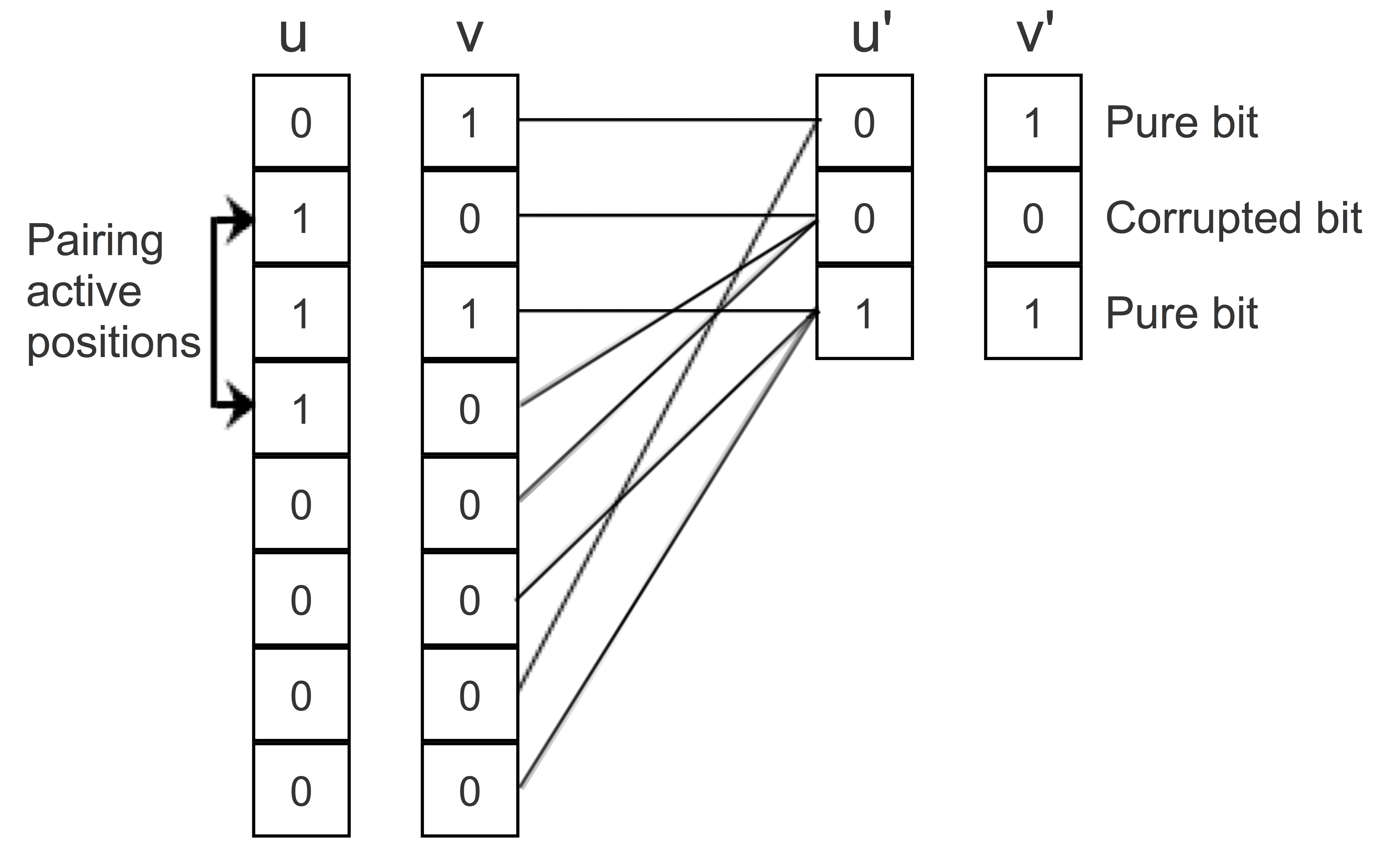
Figure 2. Illustration of pure/corrupted bits in $\mathrm{BCS}$.

Further, the deviation of Hamming distance (or Inner product similarity) between $\mathbf{u^{\prime}}$ and $\mathbf{v^{\prime}}$ from that of $\mathbf{u}$ and $\mathbf{v}$, corresponds to the number of corrupted bit positions shared between $\mathbf{u^{\prime}}$ and $\mathbf{v^{\prime}}$. Figure 2 illustrate this with an example, and the lemma below analyse it.

Lemma 2.1 (Lemma $14$ of  (KulkarniP16, )).

Consider two binary vectors $\mathbf{u},\mathbf{v}\in\{0,1\}^{d}$, which get compressed into vectors $\mathbf{u^{\prime}},\mathbf{v^{\prime}}\in\{0,1\}^{\mathrm{N}}$ using the $\mathrm{BCS}$, and suppose $\mathrm{\psi}$ is the maximum number of $1$ in any vector. Then for an integer $r\geq 1$, and $\epsilon\in(0,1)$, probability that $\mathbf{u^{\prime}}$ and $\mathbf{v^{\prime}}$ share more than $\epsilon r$ corrupted positions is at most $\left({2\mathrm{\psi}}/{\sqrt{\mathrm{N}}}\right)^{\epsilon r}.$

Proof.

We first give a bound on the probability that a particular bit position gets corrupted between $\mathbf{u^{\prime}}$ and $\mathbf{v^{\prime}}$. As there are at most $2\mathrm{\psi}$ active positions shared between vectors $\mathbf{u}$ and $\mathbf{v}$, the number of ways of pairing two active positions from $2\mathrm{\psi}$ active positions is at most $2\mathrm{\psi}\choose 2$, and this pairing will result in a corrupted bit position in $\mathbf{u^{\prime}}$ or $\mathbf{v^{\prime}}$. Then, the probability that a particular bit position in $\mathbf{u^{\prime}}$ or $\mathbf{v^{\prime}}$ gets corrupted is at most ${{2\mathrm{\psi}\choose 2}}/{{\mathrm{N}}}\leq\left({4{\mathrm{\psi}}^{2}}/{\mathrm{N}}\right).$ Further, if the deviation of Hamming distance (or Inner product similarity) between $\mathbf{u^{\prime}}$ and $\mathbf{v^{\prime}}$ from that of $\mathbf{u}$ and $\mathbf{v}$ is more than $\epsilon r$, then at least $\epsilon r$ corrupted positions are shared between $\mathbf{u^{\prime}}$ and $\mathbf{v^{\prime}}$, which implies that at least $\frac{\epsilon r}{2}$ pair of active positions in $\mathbf{u}$ and $\mathbf{v}$ got paired up while compression. The number of possible ways of pairing $\frac{\epsilon r}{2}$ active positions from $2\mathrm{\psi}$ active positions is at most ${2\mathrm{\psi}\choose\frac{\epsilon r}{2}}{2\mathrm{\psi}-\frac{\epsilon r}{2}\choose\frac{\epsilon r}{2}}\frac{\epsilon r}{2}!\leq(2\mathrm{\psi})^{\epsilon r}.$ Since the probability that a pair of active positions got mapped in the same bit position in the compressed data is $\frac{1}{\mathrm{N}}$, the probability that $\frac{\epsilon r}{2}$ pair of active positions got mapped in $\frac{\epsilon r}{2}$ distinct bit positions in the compressed data is at most $(\frac{1}{\mathrm{N}})^{\frac{\epsilon r}{2}}$. Thus, by union bound, the probability that at least $\epsilon r$ corrupted bit position shared between $\mathbf{u^{\prime}}$ and $\mathbf{v^{\prime}}$ is at most ${(2\mathrm{\psi})^{\epsilon r}}/({{\mathrm{N}}^{{\epsilon r}/{2}}})=\left({2\mathrm{\psi}}/{\sqrt{\mathrm{N}}}\right)^{\epsilon r}.$ ∎

In the lemma below generalise the above result for a set of $n$ binary vectors, and suggest a compression bound so that any pair of compressed vectors share only a very small number of corrupted bits, with high probability.

Lemma 2.2 (Lemma $15$ of  (KulkarniP16, )).

Consider a set $\mathrm{U}$ of $n$ binary vectors $\{\mathbf{u_{i}}\}_{i=1}^{n}\subseteq\{0,1\}^{d}$, which get compressed into a set $\mathrm{U^{\prime}}$ of binary vectors $\{\mathbf{u_{i}^{\prime}}\}_{i=1}^{n}\subseteq\{0,1\}^{\mathrm{N}}$ using the $\mathrm{BCS}$. Then for any positive integer $r$, and $\epsilon\in(0,1)$,

• if $\epsilon r>3\log n$, and we set $\mathrm{N}=O({\mathrm{\psi}}^{2})$, then probability that for all $\mathbf{u_{i}^{\prime}},\mathbf{u_{j}^{\prime}}\in\mathrm{U^{\prime}}$ share more than $\epsilon r$ corrupted positions is at most ${1}/{n}$.

• If $\epsilon r<3\log n$, and we set $\mathrm{N}=O({\mathrm{\psi}}^{2}\log^{2}n)$, then probability that for all $\mathbf{u_{i}^{\prime}},\mathbf{u_{j}^{\prime}}\in\mathrm{U^{\prime}}$ share more than $\epsilon r$ corrupted positions is at most ${1}/{n}$.

Proof.

For a fixed pair of compressed vectors $\mathbf{u_{i}^{\prime}}$ and $\mathbf{u_{j}^{\prime}}$, due to lemma 2.1, probability that they share more than $\epsilon r$ corrupted positions is at most $\left({2{\mathrm{\psi}}}/{\sqrt{\mathrm{N}}}\right)^{\epsilon r}.$ If $\epsilon r>3\log n$, and $\mathrm{N}=16{\mathrm{\psi}}^{2}$, then the above probability is at most $\left({2\mathrm{\psi}}/{\sqrt{\mathrm{N}}}\right)^{\epsilon r}<\left({2{\mathrm{\psi}}}/{4t}\right)^{3\log n}=\left({1}/{2}\right)^{3\log n}<{1}/{n^{3}}.$ As there are at most ${n\choose 2}$ pairs of vectors, the required bound follows from union bound of probability.

In the second case, as $\epsilon r<3\log n$, we cannot bound the probability as above. Thus, we replicate each bit position $3\log n$ times, which makes a $d$ dimensional vector to a $3d\log n$ dimensional, and as a consequence the Hamming distance (or Inner product similarity) is also scaled up by a multiplicative factor of $3\log n$. We now apply the compression scheme on these scaled vectors, then for a fixed pair of compressed vectors $\mathbf{u_{i}^{\prime}}$ and $\mathbf{u_{j}^{\prime}}$, probability that they have more than $3\epsilon r\log n$ corrupted positions is at most $\left({6\mathrm{\psi}\log n}/{\sqrt{\mathrm{N}}}\right)^{3\epsilon r\log n}$. As we set $\mathrm{N}=144{\mathrm{\psi}}^{2}\log^{2}n$, the above probability is at most $\left({6\mathrm{\psi}\log n}/{\sqrt{144{\mathrm{\psi}}^{2}\log^{2}n}}\right)^{3\epsilon r\log n}<\left({1}/{2}\right)^{3\log n}<{1}/{n^{3}}.$ The final probability follows due to union bound over all ${n\choose 2}$ pairs. ∎

After compressing binary data via $\mathrm{BCS}$, the Hamming distance between any pair of binary vectors can not increase. This is due to the fact that compression doesn’t generate any new $1$ bit, which could increase the Hamming distance from the uncompressed version. In the following, we recall the main result of (KulkarniP16, ), which holds due the above fact and Lemma 2.2.

Theorem 2.3 (Theorem $1$, $2$ of (KulkarniP16, )).

Consider a set $\mathrm{U}$ of binary vectors $\{\mathbf{u_{i}}\}_{i=1}^{n}\subseteq\{0,1\}^{d}$, a positive integer $r$, and $\epsilon\in(0,1)$. If $\epsilon r>3\log n$, we set $\mathrm{N}=O({\mathrm{\psi}}^{2})$; if $\epsilon r<3\log n$, we set $\mathrm{N}=O({\mathrm{\psi}}^{2}\log^{2}n)$, and compress them into a set $\mathrm{U^{\prime}}$ of binary vectors $\{\mathbf{u_{i}^{\prime}}\}_{i=1}^{n}\subseteq\{0,1\}^{\mathrm{N}}$ via $\mathrm{BCS}$. Then for all $\mathbf{u_{i}},\mathbf{u_{j}}\in\mathrm{U}$,

• if $\mathrm{d_{H}}(\mathbf{u_{i}},\mathbf{u_{j}})<r$, then $\Pr[\mathrm{d_{H}}({\mathbf{u_{i}}}^{\prime},{\mathbf{u_{j}}}^{\prime})<r]=1$,

• if $\mathrm{d_{H}}(\mathbf{u_{i}},\mathbf{u_{j}})\geq(1+\epsilon)r$, then $\Pr[\mathrm{d_{H}}({\mathbf{u_{i}}}^{\prime},{\mathbf{u_{j}}}^{\prime})<r]<{1}/{n}.$

For Inner product, if we set $\mathrm{N}=O({\mathrm{\psi}}^{2}\log^{2}n)$, then the following is true with probability at least $1-{1}/{n}$,

• $(1-\epsilon)\langle\mathbf{u_{i}},\mathbf{u_{j}}\rangle\leq\langle{\mathbf{u_{i}}}^{\prime},{\mathbf{u_{j}}}^{\prime}\rangle\leq(1+\epsilon)\langle\mathbf{u_{i}},\mathbf{u_{j}}\rangle.$

The following proposition relates Jaccard similarity with Inner product and Hamming distance. The proof follows as for a pair binary vectors their Jaccard similarity is the ratio of the number of positions where $1$ is appearing together, with the number of bit positions where $1$ is present in either of them. Clearly, numerator is captured by the Inner product between those pair of vectors, and denominator is captured by Inner product plus Hamming distance between them – number of positions where $1$ is occurring in both vectors, plus the number of positions where $1$ is present in exactly one of them.

Proposition 2.4.

For any pair of vectors $\mathbf{u},\mathbf{v}\subseteq\{0,1\}^{d}$, we have $\mathrm{JS}(\mathbf{u},\mathbf{v})=\langle\mathbf{u},\mathbf{v}\rangle/\left(\langle\mathbf{u},\mathbf{v}\rangle+\mathrm{d_{H}}(\mathbf{u},\mathbf{v})\right)$

In the following, we complete a proof of the Theorem 1.4 due to Proposition 2.4, and Theorem 2.3.

Proof of Theorem 1.4

Consider a pair of vectors $\mathbf{u_{i}},\mathbf{u_{j}}$ from the set $\mathrm{U}\in\{0,1\}^{d}$, which get compressed into binary vectors $\mathbf{u_{i}^{\prime}},\mathbf{u_{j}^{\prime}}\in\{0,1\}^{\mathrm{N}}$. Due to Proposition 2.4, we have $\mathrm{JS}(\mathbf{u_{i}^{\prime}},\mathbf{u_{j}^{\prime}})={\langle\mathbf{u_{i}^{\prime}},\mathbf{u_{j}^{\prime}}\rangle}/({\langle\mathbf{u_{i}^{\prime}},\mathbf{u_{j}^{\prime}}\rangle+\mathrm{d_{H}}(\mathbf{u_{i}^{\prime}},\mathbf{u_{j}^{\prime}})}).$ Below, we present a lower and upper bound on the expression.

(1) $$\mathrm{JS}(\mathbf{u_{i}^{\prime}},\mathbf{u_{j}^{\prime}}) \geq\frac{(1-\epsilon)\langle\mathbf{u_{i}},\mathbf{u_{j}}\rangle}{(1-\epsilon)\langle\mathbf{u_{i}},\mathbf{u_{j}}\rangle+\mathrm{d_{H}}(\mathbf{u_{i}},\mathbf{u_{j}})}$$

$$\geq\frac{(1-\epsilon)\langle\mathbf{u_{i}},\mathbf{u_{j}}\rangle}{\langle\mathbf{u_{i}},\mathbf{u_{j}}\rangle+\mathrm{d_{H}}(\mathbf{u_{i}},\mathbf{u_{j}})}$$

(2) $$\geq(1-\varepsilon)\mathrm{JS}(\mathbf{u_{i}},\mathbf{u_{j}})$$

Equation 1 holds hold true with probability at least $1-1/n$ due to Theorem 2.3.

$$\mathrm{JS}(\mathbf{u_{i}^{\prime}},\mathbf{u_{j}^{\prime}}) =\frac{\langle\mathbf{u_{i}^{\prime}},\mathbf{u_{j}^{\prime}}\rangle}{\langle\mathbf{u_{i}^{\prime}},\mathbf{u_{j}^{\prime}}\rangle+\mathrm{d_{H}}(\mathbf{u_{i}^{\prime}},\mathbf{u_{j}^{\prime}})}$$

(3) $$\leq\frac{(1+\epsilon)\langle\mathbf{u_{i}},\mathbf{u_{j}}\rangle}{(1+\epsilon)\langle\mathbf{u_{i}},\mathbf{u_{j}}\rangle+(1-\epsilon)\mathrm{d_{H}}(\mathbf{u_{i}},\mathbf{u_{j}})}$$

$$=\left(\frac{1+\epsilon}{1-\epsilon}\right)\frac{\langle\mathbf{u_{i}},\mathbf{u_{j}}\rangle}{\left(\frac{(1+\epsilon)}{(1-\epsilon)}\langle\mathbf{u_{i}},\mathbf{u_{j}}\rangle+\mathrm{d_{H}}(\mathbf{u_{i}},\mathbf{u_{j}})\right)}$$

$$\leq\left(\frac{1+\epsilon}{1-\epsilon}\right)\frac{\langle\mathbf{u_{i}},\mathbf{u_{j}}\rangle}{\langle\mathbf{u_{i}},\mathbf{u_{j}}\rangle+\mathrm{d_{H}}(\mathbf{u_{i}},\mathbf{u_{j}})}$$

$$=\left(1+\frac{2\epsilon}{1-\epsilon}\right)\frac{\langle\mathbf{u_{i}},\mathbf{u_{j}}\rangle}{\langle\mathbf{u_{i}},\mathbf{u_{j}}\rangle+\mathrm{d_{H}}(\mathbf{u_{i}},\mathbf{u_{j}})}$$

(4) $$\leq\left(1+\varepsilon\right)\frac{\langle\mathbf{u_{i}},\mathbf{u_{j}}\rangle}{\langle\mathbf{u_{i}},\mathbf{u_{j}}\rangle+\mathrm{d_{H}}(\mathbf{u_{i}},\mathbf{u_{j}})}$$

(5) $$=(1+\varepsilon)\mathrm{JS}(\mathbf{u_{i}},\mathbf{u_{j}})$$

Equation 3 holds hold true with probability at least $(1-1/n)^{2}\geq 1-2/n$ due to Theorem 2.3; Equation 4 holds as $\varepsilon\geq\frac{2\epsilon}{1-\epsilon}.$ Finally Equations 5 and 2 complete a proof of the Theorem.

3. Experimental Evaluation

We performed our experiments on a machine having the following configuration: CPU: Intel(R) Core(TM) i5 CPU @ 3.2GHz x 4; Memory: 8GB 1867 MHz DDR3; OS: macOS Sierra 10.12.5; OS type: 64-bit. We performed our experiments on synthetic and real-world datasets, we discuss them one-by-one as follows:

3.1. Results on Synthetic Data

We performed two experiments on synthetic dataset and showed that it preserves both: a) all-pair-similarity, and b) $k$–$\mathrm{NN}$ similarity. In all-pair-similarity, given a set of $n$ binary vectors in $d$-dimensional space with the sparsity bound $\mathrm{\psi}$, we showed that after compression Jaccard similarity between every pair of vector is preserved. In $k$–$\mathrm{NN}$ similarity, given is a query vector $\mathcal{S}_{q}$, we showed that after compression Jaccard similarity between $\mathcal{S}_{q}$ and the vectors that are similar to $\mathcal{S}_{q}$, are preserved. We performed experiments on dataset consisted of $1000$ vectors in $100000$ dimension. Throughout synthetic data experiments, we calculate the accuracy via Jaccard ratio, that is, if the set $\mathcal{O}$ denotes the ground truth result, and the set $\mathcal{O^{\prime}}$ denotes our result, then the accuracy of our result is calculated by the Jaccard ratio between the sets $\mathcal{O}$ and $\mathcal{O^{\prime}}$ – that is $\mathrm{JS}(\mathcal{O},\mathcal{O^{\prime}})={|\mathcal{O}\cap\mathcal{O^{\prime}}|}/{|\mathcal{O}\cup\mathcal{O^{\prime}}|}$. To reduce the effect of randomness we repeat the experiment $10$ times and took average.

3.1.1. Dataset generation

All-pair-similarity

We generated $1000$ binary vectors in dimension $100000$ such that the sparsity of each vector is at most $\mathrm{\psi}$. If we randomly choose binary vectors respecting the sparsity bound, then most likely every pair of vector will have similarity $0$. Thus, we had to deliberately generate some vectors having high similarity. We generated $200$ pairs whose similarity is high. To generate such a pair, we choose a random number (say $s$) between $1$ and $\mathrm{\psi}$, then we randomly select those many position (in dimension) from $1$ to $100000$, set $1$ in both of them, and set remaining to $0$. Further, for each of the vector in the pair, we choose a random number (say $s^{\prime}$) from the range $1$ to $(\mathrm{\psi}-s)$, and again randomly sample those many positions from the remaining positions and set them to $1$. This gives a pair of vectors having similarity at least $\frac{s}{s+2s^{\prime}}$ and respecting the sparsity bound. We repeat this step $200$ times and obtain $400$ vectors. For each of the remaining $600$ vectors, we randomly choose an integer from the range $1$ to $\mathrm{\psi}$, choose those many positions in the dimension, set them to $1$, and set the remaining positions to $0$. Thus, we obtained $1000$ vectors of dimension $100000$ which we used as an input matrix.

$k$–$\mathrm{NN}$– similarity

A dataset for this experiment consist of a random query vector $\mathcal{S}_{q}$; $249$ vectors whose similarity with $\mathcal{S}_{q}$ is high; and $750$ other vectors. We first generated a query vector $\mathcal{S}_{q}$ of sparsity between $1$ and $\mathrm{\psi}$, then using the procedure mentioned above we generated $249$ vectors whose similarity with $\mathcal{S}_{q}$ is high. Then we generated $750$ random vectors of sparsity is at most $\mathrm{\psi}$.

Data representation

We can imagine synthetic dataset as a binary matrix of dimension $100000\times 1000$. However, for ease and efficiency of implementation, we use a compact representation which consist of a list of lists. The the number of lists is equal to the number of vectors in the binary matrix, and within each list we just store the indices (co-ordinate) where $1$s are present. We use this list as an input for both $\mathrm{BCS}$ and minhash.

3.1.2. Evaluation metric

We performed two experiments on synthetic dataset – 1) fixed sparsity while varying compression length, and 2) fixed compression length while varying sparsity. We present these experimental results in Figures 3, 4 respectively. In both of these experiments, we compare and contrast the performance $\mathrm{BCS}$ with minhash on accuracy, compression time, and search time parameters. All-pair-similarity experiment result requires a quadratic search – generation of all possible candidate pairs and then pruning those whose similarity score is high, and the corresponding search time is the time required to compute all such pairs. While $k$–$\mathrm{NN}$– similarity experiment requires a linear search and pruning with respect to the query vector $\mathcal{S}_{q}$, and the corresponding search time is the time required to compute such vectors. In order to calculate the accuracy on a given support threshold value, we first run a simple brute-force search algorithm on the entire (uncompressed) dataset, and obtain the ground truth result. Then, we calculate the Jaccard ratio between our algorithm’s result/ minhash’s result, with the corresponding exact result, and compute the accuracy. First row of the plots are ”accuracy” vs ”compression length/sparsity”. The second row of the plots are ”compression time” vs ”compression length/sparsity”. Third row of plot shows comparison with respect to ”search time” vs ”compression length/sparsity”.

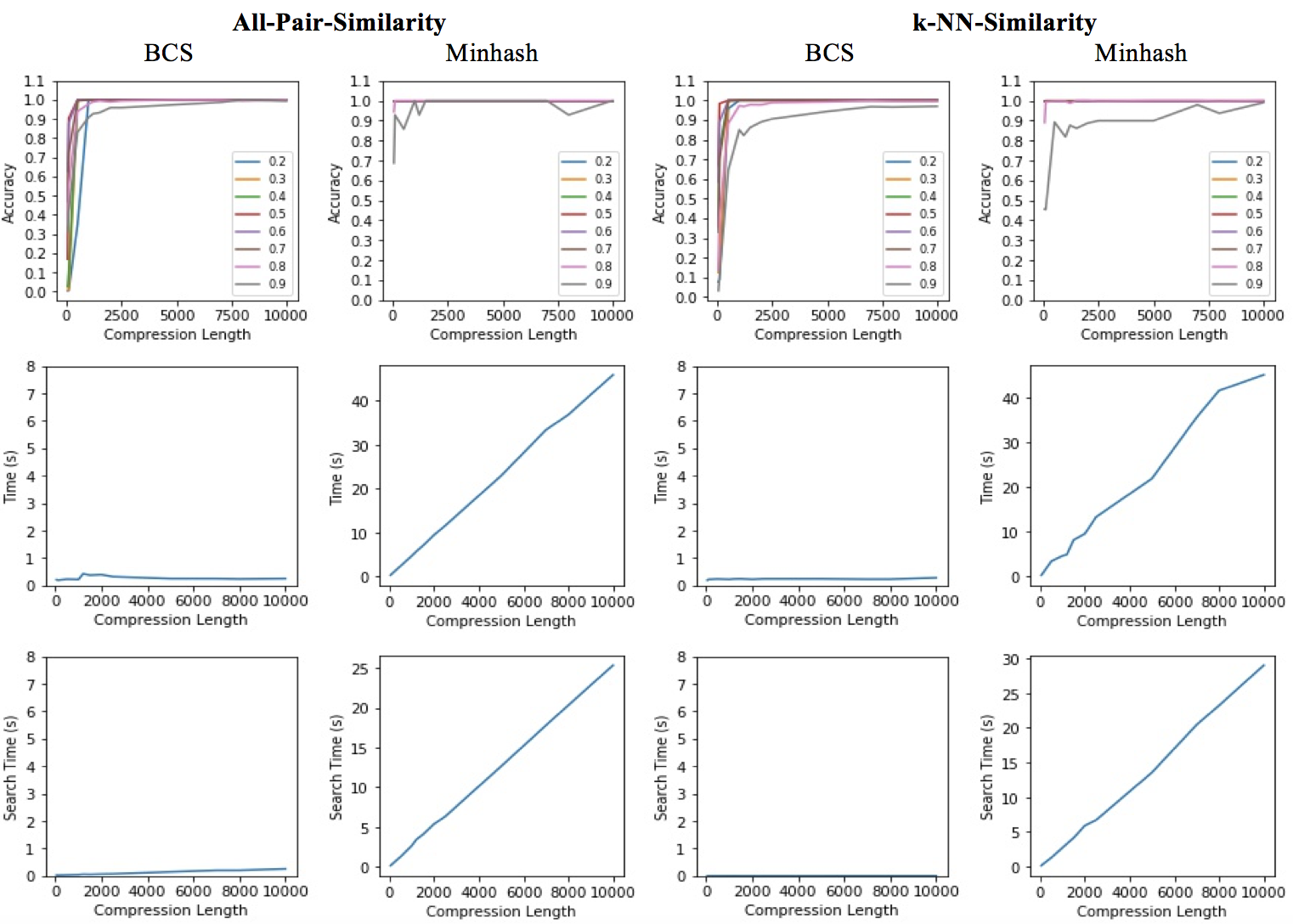
Figure 3. Experiments on Synthetic Data: for fixed sparsity $\mathrm{\psi}=200$ and varying compression length

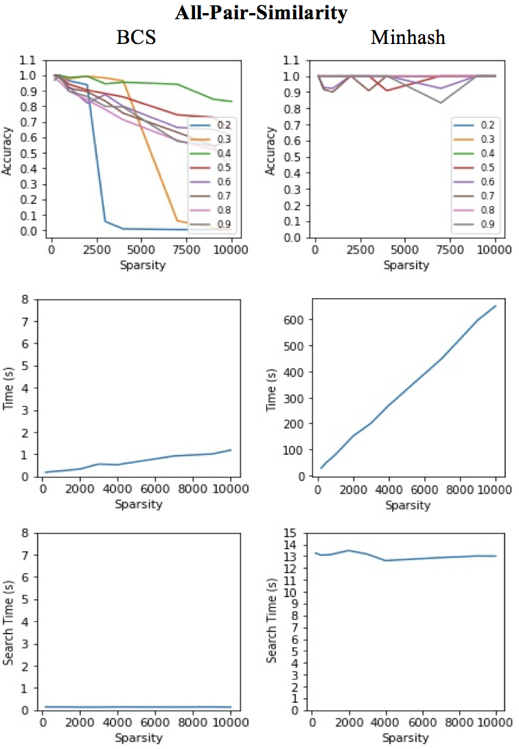
Figure 4. Experiments on Synthetic Data: for fixed compression length $5000$ and varying sparsity

3.1.3. Insight

In Figure 3, we plot the result of $\mathrm{BCS}$ and minhash for all-pair-similarity and $k$–$\mathrm{NN}$– similarity. For this experiment, we fix the sparsity $\mathrm{\psi}=200$ and generate the datasets as stated above. We compress the datasets using $\mathrm{BCS}$ and minhash for a range of compression lengths from $50$ to $10000$. It can be observed that $\mathrm{BCS}$ performs remarkably well on the parameters of compression time and search time. Our compression time remains almost constant at $0.2$ seconds in contrast to the compression time of minhash, which grows linearly to almost $50$ seconds. On an average, $\mathrm{BCS}$ is $90$ times faster than minhash. Also accuracy for $\mathrm{BCS}$ and minhash is almost equal above compression length $300$, but in the window of $50-300$ minhash performs slightly better than $\mathrm{BCS}$. Further, the search-time on $\mathrm{BCS}$ is also significantly less than minhash for all compression lengths. On an average search-time is $75$ times less than the corresponding minhash search-time. We obtain similar results for $k$–$\mathrm{NN}$– similarity experiments.

In Figure 4, we plot the result of $\mathrm{BCS}$ and minhash for all-pair-similarity. For this experiment, we generate datasets for different values of sparsity ranging from $50$ to $10000$. We compress these datasets using $\mathrm{BCS}$ and minhash to a fixed value of compression length $5000$. In all-pair-similarity, when sparsity value is below $2200$, average accuracy of BCS is above $0.85$. It starts decreasing after that value, at sparsity value is $7500$, the accuracy of $\mathrm{BCS}$ stays above $0.7$, on most of the threshold values. The compression time of $\mathrm{BCS}$ is always below $2$ seconds while compression time of minhash grows linearly with sparsity – on an average compression time of $\mathrm{BCS}$ is around $550$ times faster than the corresponding minhash compression time. Further, we again significantly reduce search time – on an average our search-time is $91$ times less than minhash. We obtain similar results for $k$–$\mathrm{NN}$– similarity experiments.

3.2. Results on Real-world Data

3.2.1. Dataset Description:

We compare the performance of $\mathrm{BCS}$ with minhash on the task of retrieving top-ranked elements based on Jacquard similarity. We performed this experiment on publicly available high dimensional sparse dataset of UCI machine learning repository (UCI, ). We used four publicly available dataset from UCI repository - namely, NIPS full papers, KOS blog entries, Enron Emails, and NYTimes news articles. These datasets are binary ”BoW” representation of the corresponding text corpus. We consider each of these datasets as a binary matrix, where each document corresponds to a binary vector, that is if a particular word is present in the document, then the corresponding entry is $1$ in that position, and it is $0$ otherwise. For our experiments, we consider the entire corpus of NIPS and KOS dataset, while for ENRON and NYTimes we take a uniform sample of $10000$ documents from their corpus. We mention their cardinality, dimension, and sparsity in Table 1.

Table 1. Real-world dataset description

Data Set	No. of points	Dimension	Sparsity
NYTimes news articles	$10000$	$102660$	$871$
Enron Emails	$10000$	$28102$	$2021$
NIPS full papers:	$1500$	$12419$	$914$
KOS blog entries	$3430$	$6906$	$457$

3.2.2. Evaluation metric:

We split the dataset in two parts $90\%$ and $10\%$ – the bigger partition is use to compress the data, and is referred as the training partition, while the second one is use to evaluate the quality of compression and is referred as querying partition. We call each vector of the querying partition as query vector. For each query vector, we compute the vectors in the training partition whose Jaccard similarity is higher than a certain threshold (ranging from $0.1$ to $0.9$). We first do this on the uncompressed data inorder to find the underlying ground truth result – for every query vector compute all vectors that are similar to them. Then we compress the entire data, on various values of compression lengths, using our compression scheme/minhash. For each query vector, we calculate the accuracy of $\mathrm{BCS}$/minhash by taking Jaccard ratio between the set outputted by $\mathrm{BCS}$/minhash, on various values of compression length, with set outputted a simple linear search algorithm on entire data. This gives us the accuracy of compression of that particular query vector. We repeat this for every vector in the querying partition, and take the average, and we plot the average accuracy for each value in support threshold and compression length. We also note down the corresponding compression time on each of the compression length for both $\mathrm{BCS}$ and minhash. Search time is time required to do a linear search on the compressed data, we compute the search time for each of the query vector and take the average in the case of both $\mathrm{BCS}$ and minhash. Similar to synthetic dataset result, we plot the comparison between our algorithm with minhash on following three points – 1) accuracy vs compression length, 2) compression time vs compression length, and 3) search time vs compression length.

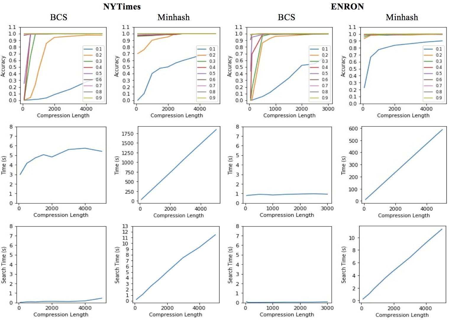
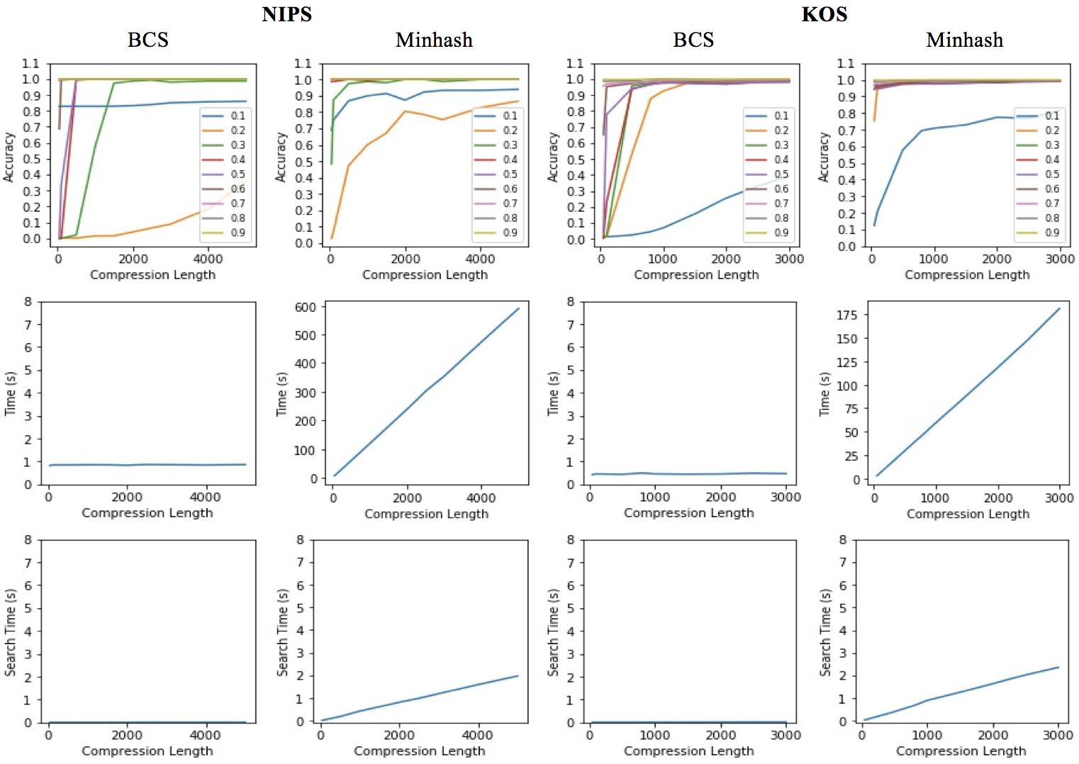
Figure 5. Experiments on Real-world datasets (UCI, ).

3.2.3. Insights

We plot experiments of real world dataset (UCI, ) in Figure 5, and found that performance of $\mathrm{BCS}$ is similar to its performance on synthetic datasets. NYTimes is the sparsest among all other dataset, so the performance of $\mathrm{BCS}$ is relatively better as compare to other datasets. For NYTIMES dataset, on an average $\mathrm{BCS}$ is $135$ times faster than minhash, and search time for $\mathrm{BCS}$ is $25$ times less than search time for minhash. For $\mathrm{BCS}$ accuracy starts dropping below $0.9$ when data is compressed below compression length $300$. For minhash, accuracy starts dropping below compression compression length $150$. Similar pattern is observed for ENRON dataset as well, where $\mathrm{BCS}$ is $268$ times faster than minhash, and a search on the compressed data obtained from $\mathrm{BCS}$ is $104$ times faster than search on data obtained from minhash. KOS and NIPS are dense, low dimensional datasets. However here also, for NIPS, our compression time is $271$ times faster and search-time is $90$ times faster as compared to minhash. For KOS, our compression time is $162$ times faster and search time is $63$ times faster than minhash.

To summarise, $\mathrm{BCS}$ is significantly faster than minhash in terms of both - compression time and search time while giving almost equal accuracy. Also, the amount of randomness required for $\mathrm{BCS}$ is also significantly less as compared to minhash. However, as sparsity is increased, accuracy of $\mathrm{BCS}$ starts decreasing slightly as compared to minhash.

4. Concluding remarks and open questions

We showed that $\mathrm{BCS}$ is able to compress sparse, high-dimensional binary data while preserving the Jaccard similarity. It is considerably faster than the ”state-of-the-art” minhash permutation, and also maintains almost equal accuracy while significantly reducing the amount of randomness required. Moreover, the compressed representation obtained from $\mathrm{BCS}$ is in binary form, as opposed to integer in case of minhash, due to which the space required to store the compressed data is reduced, and consequently leads to a faster searches on the compressed representation. Another major advantage of $\mathrm{BCS}$ is that its compression bound is independent of the dimensions of the data, and only grows polynomially with the sparsity and poly-logarithmically with the number of data points. We present a theoretical proof of the same and complement it with rigorous and extensive experimentations. Our work leaves the possibility of several open questions – improving the compression bound of our result, and extending it to other similarity measures.

References

- [1] Roberto J. Bayardo, Yiming Ma, and Ramakrishnan Srikant. Scaling up all pairs similarity search. In Proceedings of the 16th International Conference on World Wide Web, WWW 2007, Banff, Alberta, Canada, May 8-12, 2007, pages 131–140, 2007.
- [2] A. Z. Broder. On the resemblance and containment of documents. In Proceedings. Compression and Complexity of SEQUENCES 1997 (Cat. No.97TB100171), pages 21–29, Jun 1997.
- [3] Andrei Z Broder. On the resemblance and containment of documents. In Compression and Complexity of Sequences 1997. Proceedings, pages 21–29. IEEE, 1997.
- [4] Andrei Z. Broder. Identifying and filtering near-duplicate documents. In Combinatorial Pattern Matching, 11th Annual Symposium, CPM 2000, Montreal, Canada, June 21-23, 2000, Proceedings, pages 1–10, 2000.
- [5] Andrei Z. Broder. Min-wise independent permutations: Theory and practice. In Automata, Languages and Programming, 27th International Colloquium, ICALP 2000, Geneva, Switzerland, July 9-15, 2000, Proceedings, page 808, 2000.
- [6] Andrei Z. Broder, Moses Charikar, Alan M. Frieze, and Michael Mitzenmacher. Min-wise independent permutations (extended abstract). In Proceedings of the Thirtieth Annual ACM Symposium on the Theory of Computing, Dallas, Texas, USA, May 23-26, 1998, pages 327–336, 1998.
- [7] A.Z. Broder, S.C. Glassman, C.G. Nelson, M.S. Manasse, and G.G. Zweig. Method for clustering closely resembling data objects, September 12 2000. US Patent 6,119,124.
- [8] Flavio Chierichetti, Ravi Kumar, Silvio Lattanzi, Michael Mitzenmacher, Alessandro Panconesi, and Prabhakar Raghavan. On compressing social networks. In Proceedings of the 15th ACM SIGKDD International Conference on Knowledge Discovery and Data Mining, Paris, France, June 28 - July 1, 2009, pages 219–228, 2009.
- [9] Ping Li, Michael W. Mahoney, and Yiyuan She. Approximating higher-order distances using random projections. In UAI 2010, Proceedings of the Twenty-Sixth Conference on Uncertainty in Artificial Intelligence, Catalina Island, CA, USA, July 8-11, 2010, pages 312–321, 2010.
- [10] M. Lichman. UCI machine learning repository, 2013.
- [11] Rameshwar Pratap and Raghav Kulkarni. Similarity preserving compressions of high dimensional sparse data. CoRR, abs/1612.06057, 2016.