Exchange constants in molecule-based magnets derived from density functional methods

Abstract

Cu(pyz)(NO₃)₂ is a quasi one-dimensional molecular antiferromagnet that exhibits three dimensional long-range magnetic order below $T_{\mathrm{N}}=110$ mK due to the presence of weak inter-chain exchange couplings. Here we compare calculations of the three largest exchange coupling constants in this system using two techniques based on plane-wave basis-set density functional theory: (i) a dimer fragment approach and (ii) an approach using periodic boundary conditions. The calculated values of the large intrachain coupling constant are found to be consistent with experiment, showing the expected level of variation between different techniques and implementations. However, the interchain coupling constants are found to be smaller than the current limits on the resolution of the calculations. This is due to the computational limitations on convergence of absolute energy differences with respect to basis set, which are larger than the inter-chain couplings themselves. Our results imply that errors resulting from such limitations are inherent in the evaluation of small exchange constants in systems of this sort, and that many previously reported results should therefore be treated with caution.

I Introduction

Molecule-based magnets Blundell-2004 provide experimental realisations of magnetic spin systems that were, until recently, the sole preserve of theorists Lancaster-2013 . They allow an opportunity to investigate magnetism in low-dimensional systems, the occurrence of quantum critical points, the possible existence of spin liquid states, along with many other phenomena Lancaster-2013 . The theoretical characterisation and classification of these materials in terms of their dimensionality, the phases they display and their low-energy magnetic behaviour is an important part of this investigation. At low energies, the properties of a magnetic material may be mapped onto those of a magnetic spin model Whangbo-2003 ; Nova-2011 ; Moreira-2006 ; Datta-2015 , (e.g. the Heisenberg model) in which the chemical, structural and electronic properties underlying its magnetism are encoded in a small number of parameters, such as exchange constants. The diversity of possible structural and chemical arrangements allows for the synthesis of molecule-based compounds whose behaviour in this energetic limit corresponds to many different model systems. Matching a given material with the most appropriate magnetic model is therefore important if its properties are to be properly explored and understood.

Ab initio techniques such as density functional theory (DFT) Martin-2004 ; Lejaeghereaad-2016 , and semi-empirical methods based on DFT, such as some hybrid functionals or DFT+U, are often used to determine the appropriate low-energy model for a given material. This involves determining the relative energies of spin configurations, which are used to extract coupling constants. Two frequently employed methods of doing this are the dimer fragment approach (DFA) Whangbo-2003 ; Nova-2011 and the periodic approach (PA)Whangbo-2003 ; Moreira-2006 .

In the DFA it is assumed that, for a given exchange pathway between magnetic centres at sites $a$ and $b$, the most significant contributions to the exchange constant will be from only those sites and their associated ligands (that is, the exchange constant is dependent only on properties local to $a$ and $b$). Calculations (see e.g. Ref. Moreira-2006, and references therein) show that this can be a reasonable assumption, but for magnetic structures whose relative energies are small (leading, for example to exchange constants of the order of $\lesssim 0.1$ meV) it is likely that systematic errors that are introduced by focusing on a dimer fragment of the system, rather than the system as a whole, will be significant. In contrast to the DFA, the PA is the method of simulating crystalline systems using periodic boundary conditions. This is standard technology in plane-wave basis set electronic structure codes, where crystalline systems are simulated (see, for example, Ref. Payne-1992, , section IIC). Interactions between all of the electrons and nuclei of the bulk system are taken into account. More generally, for both DFA and PA, we might also ask whether we face cases where the energetic separation of different magnetic states is smaller than the energy resolution of a DFT implementation. This can lead to situations, for example, where different calculations disagree on whether a small exchange constant is ferromagnetic or antiferromagnetic, which would be reflected in very different predictions of the resulting magnetic behaviour.

In this paper, we compare properties computed using the DFA with those computed using the PA to assess the effect of significant systematic errors, whose neglect we suspect to be widespread and which are rarely addressed in the literature. The main purpose of this paper is to examine the numerical errors that are incurred in electronic structure calculations rather than the systematics of various Hamiltonians commonly used in DFT, such as (semi-)local functionals (for example PBE), non-local hybrid functionals (for example B3LYP, HSE) or Hubbard contributions (for example DFT+U). The application and performance of various functionals have been examined elsewhereMoreira-2006 ; Jornet-Somoza-2010 ; DosSantos-2016 ; feng-2004 .

We have selected the quasi one-dimensional (1D) Heisenberg antiferromagnet Cu(pyz)(NO₃)₂ (copper pyrazine dinitrate)Santoro-1970 as the basis of a case study, and perform this comparison for its three largest exchange constants. Cu(pyz)(NO₃)₂ has been chosen because it provides a good experimental realisation of the $S=1/2$ 1D antiferromagnetic Heisenberg model Villa-1971 ; Losee-1973 . As a result, its magnetic Villa-1971 ; Losee-1973 ; Mennenga-1984 ; Hammar-1999 ; Lancaster-2006 ; Jornet-Somoza-2010 , spin-dynamic Stone-2003 ; Kuhne-2009 ; Kuhne-2010 ; Kuhne-2011 ; Rohrkamp-2010 ; Gunyadin-Sen-2010 , thermal Sologubenko-2007 ; Shimshoni-2009 and vibrational Jones-2001 ; Brown-2007 properties have been the subject of experimental and theoretical investigation.

Cu(pyz)(NO₃)₂ in a coordination polymer consisting of a crystalline arrangement of chains of Cu²⁺ ions linked by pyrazine (pyz) ligands parallel to the $a$ axis of its unit cell, where each Cu²⁺ ion is also bonded to a pair of nitrate ions, illustrated in Fig. 1. The dominant magnetic exchange interaction, with exchange constant $J_{\rm d2}$ (see below), results from superexchange between the adjacent Cu²⁺ ions in each chain, mediated by the pyrazine ligands Richardson-1976 . Inter-chain magnetic interactions, often parameterised via an average inter-chain exchange constant $J^{\prime}$, are extremely weak, as suggested by magnetic susceptibility measurements Mennenga-1984 which implied $|J^{\prime}/J|<10^{-2}$. Later muon-spin relaxation measurements showed the presence of a magnetic phase transition to a regime of three dimensional long-range magnetic order (LRO) for temperatures below a Néel temperature of $T_{\mathrm{N}}=110$ mK Lancaster-2006 , leading to a revised estimate of $|J^{\prime}/J|=4.4\times 10^{-3}$. As a result of the small size of this ratio, the signature of the phase transition is not visible in specific heat measurements at low temperatures Hammar-1999 ; Sengupta-2003 ; Jornet-Somoza-2010 . A recent electron spin resonance (ESR) study Validov-2014 suggests further that the inter-chain exchange coupling in the $c$-direction may be the most important in determining the low-energy behaviour of the system, as it causes pathways in the $ac$-plane to form a frustrated triangular spin lattice.

The weak inter-chain magnetic interactions in this compound make it a suitable subject for a comparative study of the different structure methods of calculating the exchange constants. Previously, Journet-Somoza et al. Jornet-Somoza-2010 (hereafter JS) used the DFA Whangbo-2003 ; Nova-2011 to show that small changes in bond lengths between temperatures of 158 K and 2 K cause the magnetic exchange along inter-chain pathways to become significant at the lower temperature. The crystal structure at 2 K is not expected to change significantly as the temperature is lowered further, and so they argue that the topology of magnetic exchange paths that they find is valid below $T_{\mathrm{N}}=110$ mK. Dos Santos et al. DosSantos-2016 (hereafter DS) have carried out DFA calculations using the crystal structure measured at 100 K using the same exchange functional, along with a calculation of the strongest coupling using the PA. Their results are consistent with those of JA. It is notable that several of the exchange constants calculated in these studies are relatively small, of the order of 10^-2 times smaller than the leading order exchange, and it is therefore possible that the values of these constants could be sensitive to systematic errors.

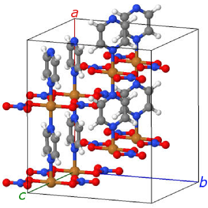
Figure 1: Structure of the Cu(pyz)(NO₃)₂ unit cell at $T=2$ K, as used in the PA calculation. Gold indicates the Cu ions, red O, blue the N, grey C and white H.Jornet-Somoza-2010 .

The sensitivity of the exchange constants to numerical and systematic error are examined here for Cu(pyz)(NO₃)₂ at 2 K within the framework of a plane wave GGA+U Martin-2004 approach using both the DFA and the PA. Below we discuss the implications of our results on the accuracy of these approaches and the nature of the long-range magnetic order of Cu(pyz)(NO₃)₂ at low temperature.

II Method

To extract the Heisenberg coupling constants, we employ a collinear magnetic model where ordered spins are constrained to adopt parallel or antiparallel configurations. Our approach involves determining the energy differences between ordered spin states that differ by a number of reversed spins. An underlying physical assumption, therefore, is that upon magnetically ordering, the magnetic structure is constrained to be collinear. In other words, the value of the magnetic exchange derived assumes that nearest neighbor spins $\bm{S}$ at sites $i$ and $j$ obey $\bm{S}_{i}\cdot\bm{S}_{j}=\pm 1$. If this is not the case, then the error in this assumption is absorbed into the value of the exchange constant that is derived. More specifically, we map the magnetic centres of the system to an Ising Hamiltonian Whangbo-2003 ; Nova-2011 ; Moreira-2006

$$\hat{H}_{\rm Ising}=-2\sum_{i>j}I_{ij}S_{z\,i}S_{z\,j}.$$ (1)

Here, $I_{ij}$ is the exchange constant parameterizing the interaction between the magnetic centres (in this case the Cu²⁺ ions) labeled by $i,j$ and $\hat{S}_{z\,i}$ is the Ising spin operator for site $i$. The coupling constants $I_{ij}$ are calculated by relating the energies of the ferromagnetic (FM) ordered state and the various antiferromagnetic (AFM) ordered states found using the DFA or PA method. We convert an Ising coupling $I_{ij}$ for a given pathway to the desired Heisenberg coupling $J_{ij}$ for that pathway using Datta-2015

$$J_{ij}=\frac{I_{ij}}{N_{\rm mc}},$$ (2)

where $N_{\rm mc}$ is the number of magnetic centres in the unit cell (or supercell) used in the calculation.

II.1 Dimer Fragment Approach

In the DFA Whangbo-2003 ; Nova-2011 ; Moreira-2006 , the system is divided into pairs of magnetic centres corresponding to magnetic exchange pathways. In many cases Moreira-2006 the value of the exchange constant linking those centres can be described accurately using only the two centres and their corresponding ligands. It is then reasonable to assume that the value of the exchange constant may be calculated using a model consisting of an isolated system that includes only those components. We select isolated dimer fragments of the system that correspond to the three largest exchange pathways, illustrated in Fig. 2, and obtain the value of the exchange coupling, $J$, along a particular pathway by relating the FM and AFM energies of the corresponding Ising dimer system via

$$J=\frac{E_{\rm AFM}-E_{\rm FM}}{2},$$ (3)

where $E_{\rm AFM}$ is the energy of the dimer in an antiferromagnetic spin configuration and $E_{\rm FM}$ is the energy of the ferromagnetic configuration.

We use the labeling conventions of Ref. Jornet-Somoza-2010, , where $J_{\mathrm{d}1}$ is the exchange coupling along the $b$-direction, $J_{\mathrm{d}2}$ the exchange along the $a$-direction and $J_{\mathrm{d}3}$ the exchange along the $c$-direction. The parameter $J_{\mathrm{d}2}$ is therefore the value of the superexchange coupling between magnetic sites along the Cu-pyz-Cu chains and determines the energy scale of the 1D behaviour of the system at temperatures $T_{N}\leq T\lesssim J$ SachdevBook . The couplings $J_{\mathrm{d}1}$ and $J_{\mathrm{d}3}$ contribute to the 3D magnetic ordering behaviour of the system on cooling towards $T_{\mathrm{N}}=110$ mK. The relative strengths of the three couplings will determine the properties of the low temperature LRO. The structure they describe is that of a stacked triangular lattice Collins-1997 and so effects related to spin frustration in the $ac$ plane may arise if $J_{\mathrm{d}3}/J_{\mathrm{d}2}$ is sufficiently large.

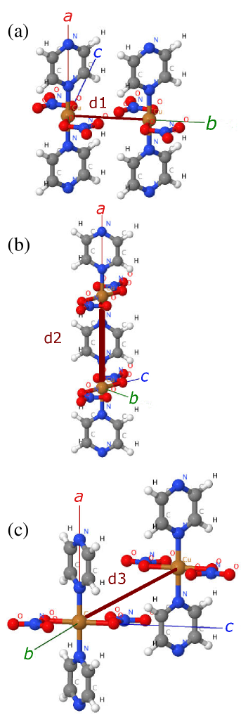
Figure 2: Exchange pathways used in Ref. Jornet-Somoza-2010, . (a) d1 (directed along the $b$-axis), (b) d2 (along the $a$-axis), (c) d3 (along the $c$-axis).

II.2 Periodic Approach

In the PA Whangbo-2003 ; Moreira-2006 we map the magnetic structure of the compound to the model depicted in Fig. 3(a) where $\hat{a}$, $\hat{b}$ and $\hat{c}$ give a shift by one site in the directions a, b and c respectively. Calculations are performed for a periodic unit cell containing eight Cu ions [see Figs. 1 and 3(b)], which is the smallest number of Cu ions needed to realize enough spin configurations to calculate $J_{\mathrm{d}1},\,J_{\mathrm{d}2}$ and $J_{\mathrm{d}3}$.

Comparing Eq. (1) and Fig. 3(a), we write the Ising Hamiltonian of the system as

$$\hat{H}=\hat{H}_{d1}+\hat{H}_{d2}+\hat{H}_{d3},$$ (4)

where

$$\hat{H}_{d1} = -2I_{d1}\sum_{i=1}^{n}\hat{S}_{z\,i}\hat{S}_{z\,i+\hat{b}},$$

$$\hat{H}_{d2} = -2I_{d2}\sum_{i=1}^{n}\hat{S}_{z\,i}\hat{S}_{z\,i+\hat{a}},$$

$$\hat{H}_{d3} = -2I_{d3}\sum_{i=1}^{n}\left(\hat{S}_{z\,i}\hat{S}_{z\,i+\hat{c}}+\hat{S}_{z\,i+\hat{c}}\hat{S}_{z\,i+\hat{a}}\right).$$ (5)

Here, $n$ is the total number of lattice sites. Note that $H_{d3}$ explicitly defines a triangular exchange topology, as can be seen from Fig. 3(a).

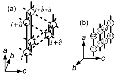
Figure 3: (a) The Ising model mapping of the chain is illustrated showing the magnetic centres, superexchange pathways (full lines) and direct exchange pathways (broken lines). Vectors $\hat{a}$, $\hat{b}$ and $\hat{c}$ indicate hopping in that direction by a single magnetic site. (b) Schematic of Fig. 1 showing only the Cu²⁺ ions, the superexchange pathways along the chains and the labeling convention used for spin configurations.

State	Label	Energy
00000000	FM	$E_{\rm FM}=-4J_{\mathrm{d}1}-4J_{\mathrm{d}2}-8J_{\mathrm{d}3}$
01101001	AFM1	$E_{\rm AFM1}=4J_{\mathrm{d}1}+4J_{\mathrm{d}2}$
01011010	AFM2	$E_{\rm AFM2}=4J_{\mathrm{d}1}+4J_{\mathrm{d}2}$
01100110	AFM3	$E_{\rm AFM3}=-4J_{\mathrm{d}1}+4J_{\mathrm{d}2}$
00111100	AFM4	$E_{\rm AFM4}=4J_{\mathrm{d}1}-4J_{\mathrm{d}2}+8J_{\mathrm{d}3}$

Table 1: Energies for spin configurations of the unit cell shown in Fig. 1. These states are degenerate with those resulting from the reversal of all spins.

Using the labeling convention of Fig. 1 and Fig. 3(b), we denote different ordered spin configurations we have calculated as a list of 0s (spin down) and 1s (spin up) in the order A₁A₂B₁B₂C₁C₂D₁D₂. Table 1 lists trial ferromagnetic (FM) and antiferromagnetic states (AFM1, AFM2, AFM3, and AFM4), and how these are related to the exchange constants. Note that AFM1 and AFM2 are degenerate; we label their energy as $E_{\rm AFMG}$. From the expressions for the energy of the configurations, the exchange constants Datta-2015 are obtained via

$$J_{\mathrm{d}1} = \frac{E_{\rm AFMG}-E_{\rm AFM3}}{64},$$

$$J_{\mathrm{d}2} = \frac{E_{\rm AFM3}-E_{\rm FM}}{64},$$

$$J_{\mathrm{d}3} = \frac{E_{\rm AFM4}+E_{\rm AFM3}-E_{\rm FM}-E_{\rm AFMG}}{128}.$$ (6)

II.3 Numerical Details

	PA	DFA
		d1	d2	d3
a (Å)	13.383	21.440	28.631	25.286
b (Å)	10.211	21.788	16.683	16.683
c (Å)	11.600	19.397	19.394	27.194

Table 2: Lattice parameters and convergence criteria used for the calculations.

All calculations were carried out using the CASTEP electronic structure packageCASTEP with accurate Lejaeghereaad-2016 ‘on-the-fly’ ultrasoft, PBE Perdew-1996 pseudo-potentials. The cell sizes used are summarised in Table 2. The DFA requires that the dimers used in the calculation are isolated. This was simulated in a pseudo-periodic approach by choosing cell dimensions so that each periodic image of the fragment is separated by sufficient vacuum to be isolated, as discussed in the Supplemental Informationsi .

Recent work on the comparison of different implementations of DFT Lejaeghereaad-2016 discuss the quantity $\Delta$, which is a measure of the difference in converged quantities, particularly energy, between different DFT implementations. These indicate that the best $\Delta$ values across a range of DFT implementations are of the order of 0.5 meV/atom therefore when examining small total energies there are implementation differences which indicate a limit to the absolute accuracy. However energy differences within a particular implementation are more accurate as some error cancellation occurs.

To that end, total energy differences are converged with respect to basis set size (Monkhorst-Pack (MP) gridsMonkhorst-1976 , plane wave cutoff and appropriate spatial discretisations) to a higher tolerance than usual, being accurate to better than 0.1 meV/cell. This is the value that limits the accuracy on energy differences and hence coupling constants. The self-consistent eigenvalues are converged to $10^{-12}$ eV to ensure that self-consistency in the calculation does not impose additional numerical error. Details are given in the Supplemental Information.

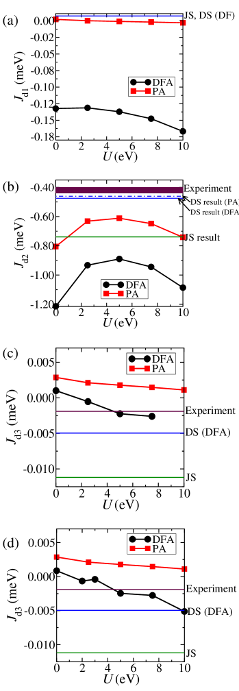
Figure 4: Calculated exchange constants compared with other computational and experiment data for (a) $J_{\rm d1}$; (b) $J_{\rm d2}$; (c) $J_{\rm d3}$; (d) $J_{\rm d3}$ with a larger unit cell size. Experimental results in (b) are from magnetic susceptibility measurements Hammar-1999 and in (c) are ESR Validov-2014 .

III Results

III.1 Exchange Constants

The differences we find in the calculated energies for the different spin structures are very small, reflecting the weakness of the inter-chain exchange constants compared to the dominant intra-chain exchange. Figure 4 shows our results for the exchange couplings compared to results from earlier work Jornet-Somoza-2010 ; DosSantos-2016 and experimental estimates Hammar-1999 ; Validov-2014 .

First we examine the largest exchange coupling $J_{\rm d2}$ [Fig. 4 (b)], which corresponds to the exchange along the Cu-pyz-Cu chains. We note that both our DFA and PA calculations both predict AFM coupling and are comparable with both previous calculations and the values derived from magnetic susceptibility measurements.Hammar-1999

Although no single calculation reproduces the experimental value, (i) the DS results, calculated using both PA and DFA, provide the best agreement, followed by (ii) our PA result evaluated with $U=5.0$ eV, (iii) the JS result and (iv) our DFA calculation evaluated at $U=5.0$ eV. For $0\leq U<5.0$ eV, our PA and DFA values approach the experimental value as $U$ is increased. Above $U=5.0$ eV, we see that $J_{\rm d2}$ decreases, departing from the experimental value as $U$ is further increased, and that at $U=10.0$ eV the PA result is close to the JS value. The best agreement with experiment from our calculations is obtained at $U=5.0$ eV for both methods, with the PA giving the closer agreement. Since $U=5.0$ eV gives the best match of $J_{\rm d2}$ to the experimentally measured values, we empirically fix this value to compare the calculated exchange constants at $U=5$ eV to the results of previous calculations in Table 3.

We may summarize that the calculated values of the principal exchange constant $J_{\mathrm{d2}}$ lie above the predicted limit of the energy resolution of our well-converged calculations ($\approx 0.1$ meV/cell) and the variation between our results and the previous ones lie within the expected variation for different implementations ($\approx 0.5$ meV/atom). It is also notable that the difference between our PA and DFA results is also of this order. This is discussed further in Section IV

The most notable property of the other coupling constants ($J_{\mathrm{d1}}$ and $J_{\mathrm{d3}}$) is that they are found to be very small compared to $J_{\mathrm{d2}}$. No experimental results are available for $J_{\rm d1}$ but both JS and DS predict FM coupling [Fig 4(a)]. In contrast, our DFA results indicates AFM coupling, while our PA calculation gives a coupling very close to zero, with $J_{\rm d1}$ changing sign between $U=2.5$ eV and $U=5.0$ eV, going from FM coupling to AFM coupling. The results for $J_{\rm d3}$ [Fig. 4(c)] show that both our PA and DFA exchange constants decrease with increasing $U$. Our PA data indicate a FM coupling while in the DFA a small FM coupling that evolves into a small AFM coupling which, at $U=5.0$ eV, is close the ESR-derived estimateValidov-2014 . [We note in passing that the $U=10.0$ eV result for the DFA calculation ($J_{\rm d3}=0.024$ meV) is omitted from Fig. 4(c), since its behaviour is a consequence of the large $U$ value giving the system a different ground state, and cannot then be compared with the other results. Increasing the vacuum spacing by expanding the cell dimensions in all directions by 2.5 Å  [Fig. 4 (d)] causes the $U=10.0$ eV value to become an AFM exchange constant. The resulting similarity between the values in Fig. 4(c) and Fig. 4(d) justifies the use of the smaller cell.]

To summarize the results from the subdominant exchange couplings, we note that the absolute magnitude predicted for these constants is small compared to the 0.1 meV/cell resolution limit we predict for the calculations, leading us to doubt that they are meaningful. This is discussed in more detail below (see Section IV), but immediately suggests that any attempt to derive even the qualitative behaviour of the system will fail owing to the changes in sign of these quantities.

Exchange	JS Jornet-Somoza-2010	DS DosSantos-2016	DFA	PA
pathway			$U=5.0$ eV	$U=5.0$ eV
$J_{\mathrm{d}1}$ ($\times 10^{-4}$ eV)	$0.07$	$0.07$	$-0.14$	$-0.02$
$J_{\mathrm{d}2}$ ($\times 10^{-4}$eV)	$-7.39$	$-4.61$ (PA), $-4.75$ (DFA)	$-8.90$	$-6.61$
$J_{\mathrm{d}3}$ ($\times 10^{-4}$eV)	$-0.11$	$-0.02$	$-0.04$	$0.14$

Table 3: Comparison of our results with those of Refs. Jornet-Somoza-2010, and DosSantos-2016, .

III.2 Energy levels and band structures

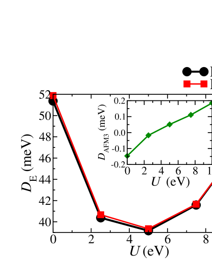
Figure 5: Plots of the relative energies per supercell $D_{\rm E}=E_{\rm E}-E_{\rm AFMG}$.

An immediate consequence of the small differences in the energies of the low-lying magnetic states is that it is difficult to reliably determine the predicted ground state magnetic spin structure. Fig. 5 shows the separation of energies $D_{\rm E}$ (where ${\rm E}$ labels the states ${\rm AFM3,\,AFM4,\,FM}$) relative to the energy of the low-lying AFMG state. We see that both $D_{\rm AFM4}$ and $D_{\rm FM}$ follow roughly parabolic behaviour as $U$ increases, with a minimum in energy difference of $D_{\rm AFM4,FM}\approx 0.039$ meV occurring at $U=5.0$ eV. These two quantities are very similar in value at $U=0$ and become more so as $U$ increases. In comparison $D_{\rm AFM3}$ is found to be small (less than $\pm 0.2$ meV) and is negative until a point $U_{\mathrm{c}}$ between $U=2.5$ eV and $U=5.0$ eV, where it becomes positive. This implies that below $U_{\mathrm{c}}$ the magnetic ground state structure of that system is predicted to be AFM3; while it is predicted to be the AFMG state above $U_{\mathrm{c}}$.

Details of the electronic structure of these magnetic systems is shown in the band structures at $U=5.0$ eV, displayed in Fig. 6. Qualitatively, the bands closest to the Fermi energy in AFM3 [Fig. 6 (b)] and AFMG [Fig. 6(a)] have similar band structures and density of states $g(\varepsilon)$, but with some small additional splitting of degeneracies visible in the AFM3 bands. Apart from a standard splitting in spin channel energies, the FM band structure [Fig. 6(d)] shows that the states closest to the Fermi energy are qualitatively very similar to AFM4 [Fig. 6 (c)]. (In the latter case the density of states plots are noticeably different, since the spins in the FM case are only oriented in one direction.) The band structures of the AFM3/AFMG and FM/AFM4 groups are qualitatively different from each other, which is consistent with the small energy separation between the AFM3 and AFMG states on the one hand, and the FM and AFM4 states on the other, as well as the large energy separation between the AFMG and the AFM4 and FM states.

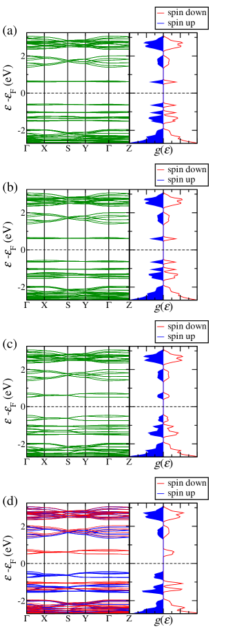
Figure 6: Band structure and density of states $g(\epsilon)$ for (a) AFMG, (b) AFM3, (c) AFM4 and (d) FM magnetic states.

IV Discussion

Although DFT+U yields results that are able to describe a range of magnetic structures in this system, all calculations make use of approximations that will give rise to error. From Fig. 5 we see that this is particularly significant for structures such as AFMG and AFM3 (or AFM4 and FM), which are very close in energy. It is the energy differences in Eqs. (6) that determine the $J$-couplings and hence it is the errors in these energy differences that determine the reliability of the results. The magnitudes of the energy differences between the FM and AFM4 states and the AFM3 and AFMG states are small (predicted to be fractions of 1 meV/atom). When one compares these to absolute energy convergence with respect to basis set (k-points, energy cutoff and spacial grids), predicted to be of order 0.1 meV/cell, errors are both inevitable and likely to be large relative to the calculated values of the small exchange constants. Due to these considerations we have no grounds to expect calculations using different implementations of the calculation or different techniques to agree on the values of these exchange constants.

An additional source of approximation in the DFA is that arising from the truncation of the full crystal structure down to a pair of magnetic centres. This neglects the contributions to the exchange constant that might arise from neighbouring magnetic centres. Furthermore, the confinement of electrons within a smaller subsystem of the chemical structure will tend to increase their kinetic energy relative to that of electrons in the full structure, much as the energy of an electron confined in a box is larger if the dimensions of the box are made smaller. These effects will only be significant if they are of similar order to the magnitude of the exchange constant. For the dominant exchange pathway this will not usually be the case, which is why this approach can produce qualitatively accurate results for these couplings that are comparable with the results of the PA method [as seen in Fig. 4(b) for $J_{\rm d2}$], and why the trimer cluster calculation of JS Jornet-Somoza-2010 did not produce a qualitatively different result from their dimer calculation.

It is clear that calculations of subdominant Heisenberg exchange constants of the order of 0.01 meV calculated using a single method and/or exchange-correlation functional should not be taken at face value, as the calculations are not converged enough with respect to basis set. A reliable conclusion that can be drawn is merely that these exchange constants are small compared to the energy resolution of the calculation method.

V Conclusion

We have calculated the three largest magnetic exchange constants in Cu(pyz)(NO₃)₂ using well-converged, plane wave density functional methods, augmented by a Hubbard-U approach, using two different structural models. The results of both are qualitatively consistent with each other and experiment for the dominant nearest neighbour exchange constant $J_{\mathrm{d}2}$. However this does not hold true for the smaller $J_{\mathrm{d}1}$ and $J_{\mathrm{d}3}$ exchange constants, for which different calculational approaches and implementations of DFT may give qualitatively different results. This is because the difference in energy between several magnetic states of this system is small enough that it cannot be reliably resolved by state-of-the-art DFT implementations. For the very small coupling constants, we should not expect consistency between calculations that use different functionals, for example as $U$ varies. The small exchange constants in Cu(pyz)(NO₃)₂ determine the nature of the 3D LRO that occurs below $T_{\mathrm{N}}=110$ mK. Since the different techniques discussed in this paper give different values of the inter-chain exchange constants, they also imply different magnetic ground states. To the extent that we are uncertain as to the value of these exchange constants, we are uncertain as to the true LRO of the system at low temperatures.

It is also worth noting that here that the use of hybrid density functionals will not lead to any improvement in the accuracy of the interchain couplings. (The results calculated in Refs DosSantos-2016, and Jornet-Somoza-2010, involved the use of such hybrid functionals.) We have demonstrated that the main source of error in the calculation of coupling constants is numerical precision and the numerical precision using hybrid functionals is significantly worse than using density-based functionals. This is because in calculating (and hence converging) total energies, the error is first order on the wavefunction and second order on the density. As an aside, it should be noted that nearly all hybrid functionals have free parameters that are often empirically fitted. These unconstrained functionals sacrifice physical rigor for the flexibility of such empirical fitting and have been shown to be becoming less accurate with time Medvedev-2017 .

More generally, low dimensional molecule-based magnets are usually characterized by one relatively large exchange constant $J$ that determines the energy scale of the low-dimensional behaviour expected to occur for $T_{\mathrm{N}}<T<J$, and several smaller ones that will determine the ordering temperature $T_{\mathrm{N}}$ and the magnetic ground state of the system. The smaller the values of the subdominant exchange constants in a particular material, the more successful a realization of a low-dimensional spin model. It is worth noting that the reliable experimental determination of the small, subdominant exchange constants in molecular magnets is generally quite difficult. It is often not possible to extract them uniquely from fits of the temperature dependence of magnetic susceptibility, for example, and so their magnitude must be estimated from combining measurements of the magnetic ordering temperature with the results of modeling (e.g. from quantum Monte Carlo simulations) Lancaster-2006 . In cases where there are several small couplings, perhaps differing in sign, more sophisticated fitting of neutron scattering results could yield the different couplings, although such measurements generally require large single crystals and the deuteration of the material, which has been shown to subtly alter the magnetic properties maitland . In DFT+U and related theoretical approaches, the extreme sensitivity of the small exchange constants to errors (that do not affect the value of the leading order constant) is likely to be a general problem in reliably applying DFT to these systems. It is likely, therefore, that the values of many of the smallest exchange constants determined using DFT methods (including ab initio XC functionals, semi-empirical hybrid functionals and DFT+U) are little more than an artefact of the implementation or convergence criteria, rather than the result of controlled approximations.

VI Acknowledgments

This work was funded by EPSRC and the John Templeton Foundation as part of the Durham Emergence Project. We would like to thank the UK Car-Parrinello collaboration for computer time. Calculations were performed using the ARCHER, N8 Polaris, and the Hamilton (Durham) HPC facilities. Research data from this paper will be made available via Durham Research Online.

References

- (1) S. J. Blundell and F. L. Pratt, J. Phys. Condens. Matter , R771 (2004).
- (2) T. Lancaster, S. J. Blundell, and F. L. Pratt, Physica Scripta 88, 068506 (2013).
- (3) M.-H. Whangbo, H.-J. Koo, and D. Dai, J. Solid State Chem. 176, 417 (2003).
- (4) J. J. Nova, M. Deumel, and J. Jornet-Somozoa, Chem. Soc. Rev. 40, 3182 (2011).
- (5) I. de P. R. Moreira and F. Illas, Phys. Chem. Chem. Phys. 8, 1645 (2006).
- (6) S. N. Datta and S. Hansda, Chem. Phys. Lett. 621, 102 (2015).
- (7) R. M. Martin, Electronic Structure: Basic Theory and Practical Methods, Cambridge University Press, 2004.
- (8) K. Lejaeghere et al., Science 351, aad3000, (2016), doi=10.1126/science.aad3000.
- (9) M.C. Payne, M. P. Teter, D. C. Allan, T. A. Arias, and J. D. Joannopoulos, Rev. Mod. Phys. 64, 1045 (1992).
- (10) L. H. R. D. Santos, A. Lanza, A. M. Barton, J. Brambleby, W. J. A. Blackmore, P. A. Goddard, F. Xiao, R. C. Williams, T. Lancaster, F. L. Pratt, S. J. Blundell, J. Singleton, J. L. Manson, and P. Macchi J. Am. Chem. Soc. 138, 2280 (2016).
- (11) J. Journet-Somoza, M. Deumal, M. A. Robb, C. P. Landee, M. M. Turnbull, R. Feyerher¶ and J. J. Novoa, Inorg. Chem. 49, 1750 (2010).
- (12) X. Feng and N.M. Harrison, Phys. Rev. B 70, 092402 (2004).
- (13) A. Santoro, A. D. Mighell, and C. W. Riemann, Acta Cryst. B 26, 979 (1970).
- (14) J. F. Villa and W. E. Hatfield, J. Am. Chem. Soc 93, 4081 (1971).
- (15) D. B. Losee, H. W. Richardson, and W. E. Hatfield, J. Chem. Phys. 59, 3600 (1973).
- (16) G. Mennenga, L. J. de Jongh, W. J. Huiskamp, and J. Reedijk, J. Magn. Magn. Mater. 44, 89 (1984).
- (17) P.R. Hammar, M.B. Stone, D.H. Reich, C. Broholm, P.J. Gibson, M.M. Turnbull, C.P. Landee and M. Oshikawa, Phys. Rev. B 59, 1008 (1999).
- (18) T. Lancaster, S.J. Blundell, M.L. Brooks, P.J. Baker, F.L. Pratt, J.L. Manson, C.P. Landee and C. Baines, Phys. Rev. B 73, 020410(R) (2006).
- (19) M.B. Stone, D.H. Reich, C. Broholm, K. Lefmann, C. Rischel, C.P. Landee and M.M. Turnbull, Phys. Rev. Lett. 91, 037205 (2003).
- (20) H. Kühne, H.H. Klauss, S. Grossjohann, W. Brenig, F.J. Litterst, A.P. Reyes, P.L. Kuhns, M.M. Turnbull, and C.P. Landee, Phys. Rev. B 80, 045110 (2009).
- (21) H. Kühne, M. Gn̈ther, S. Grossjohann, W. Brenig, F. J. Litterst, A. P. Reyes, P. L. Kuhns, M. M. Turnbull, C. P. Landee and H.-H. Klauss, Phys. Status Solidi B 247, 671 (2010).
- (22) H. Kühne, A.A. Zvyagin, M. Gunther, A.P. Reyes, P.L. Kuhns, M.M. Turnbull, C.P. Landee and H.H. Klauss, Phys. Rev. B 83, 100407(R) (2011).
- (23) J. Rohrkamp, M. D. Phillips, M. M. Turnbull, and T. Lorenz, Thermal expansion of the spin- heisenberg-chain compound cu(c4h4n2)(no3)2, in J. Phys.: Conf. Ser., volume 200, page 012169, 2010.
- (24) O. Günaydın-Şen, C. Lee, L. C. Tung, P. Chen, M. M. Turnbull, C. P. Landee, Y. J. Wang, M.-H. Whangbo, and J. L. Musfeldt Phys. Rev. B 81, 104307 (2010).
- (25) A.V. Sologubenko, K. Berggold, T. Lorenz, A. Rosch, E. Shimshoni, M.D. Phillips and M.M. Turnbull, Phys. Rev. Lett. 98, 107201 (2007).
- (26) E. Shimshoni, D. Rasch, P. Jung, A. V. Sologubenko, and A. Rosch, Phys. Rev. B 79, 064406 (2009).
- (27) B. R. Jones, P. A. Varughese, I. Olejniczak, J. M. Pigos, J. L. Musfeldt, C. P. Landee, M. M. Turnbull, and G. L. Carr Chem. Mater. 13, 2127 (2001).
- (28) S. Brown, J. Cao, J. L. Musfeldt, M. M. Conner, A. C. McConnell, H. I. Southerland, J. L. Manson, J. A. Schlueter, M. D. Phillips, M. M. Turnbull and C. P. Landee Inorg. Chem. 46, 8577 (2007).
- (29) H. W. Richardson and W. E. Hatfield, J. Am. Chem. Soc. 98, 835 (1976).
- (30) P. Sengupta, A. W. Sandvik, and R. R. P. Singh, Phys. Rev. B 68, 094423 (2003).
- (31) A. A. Validov, M. Ozerov, J. Wosnitza, S. A. Zvyagin, M. M. Turnbull, C. P. Landee and G. B. Teitel’baum J. Phys.: Cond. Matt. 26, 026003 (2014).
- (32) S. Sachdev, Quantum Phase Transitions Second Edition, Cambrige University Press, Cambridge, New York, 2011.
- (33) M. F. Collins and O. A. Petrenko, Can. J. Phys. 75, 605 (1997).
- (34) S. J. Clark, M. D. Segall, C. J. Pickard, P. J. Hasnip, M. I. J. Probert, K. Refson and M. C. Payne Zeit. fuer Krist. 220, 567 (2005).
- (35) J.P Perdew, K. Burke, and M. Ernzerhof, Phys. Rev. Lett. 77, 3865 (1996).
- (36) H. Monkhorst and J. Pack, Phys. Rev. B 13, 5188 (1976).
- (37) The Supplemental Information includes discussion of the separation required for dimers and along with converged parameters for both DFA and PA calculations.
- (38) M.G. Medvedev, I.S. Bushmarinov, J, Sun, J.P. Perdew and K.A. Lyssenko Science, 355 49 (2017).
- (39) P. A. Goddard, J. Singleton, C. Maitland, S. J. Blundell, T. Lancaster, P. J. Baker, R. D. McDonald, S. Cox, P. Sengupta, J. L. Manson, K. A. Funk, and J. A. Schlueter Phys. Rev. B 78, 052408 (2008).