Sequence selection by dynamical symmetry breaking in an autocatalytic binary polymer model

Abstract

Template directed replication of nucleic acids is at the essence of all living beings and a major milestone for any origin of life scenario. We here present an idealized model of prebiotic sequence replication, where binary polymers act as templates for their autocatalytic replication, thereby serving as each others reactants and products in an intertwined molecular ecology. Our model demonstrates how autocatalysis alters the qualitative and quantitative system dynamics in counter-intuitive ways. Most notably, numerical simulations reveal a very strong intrinsic selection mechanism that favors the appearance of a few population structures with highly ordered and repetitive sequence patterns when starting from a pool of monomers. We demonstrate both analytically and through simulation how this “selection of the dullest” is caused by continued symmetry breaking through random fluctuations in the transient dynamics that are amplified by autocatalysis and eventually propagate to the population level. The impact of these observations on related prebiotic mathematical models is discussed.

I Introduction

The ability of nucleic acids to serve as templates for their own replication via the well-known Watson-Crick pairing is at the heart of all life known today. Consequently, the onset of such chemical sequence information and its replication are crucial cornerstones in most theories about the origin of life Eigen (1971); Gilbert (1986).

While the appearance of first molecular replicators is still subject to ongoing debate Monnard (2008); Powner et al. (2009), we suspect DeClue et al. (2009); Rasmussen et al. (2016) that catalysis combined with replication of the catalytic molecules is the critical molecular invention. Catalysis enables access to energy and resources while replication both preserves and enables combinatorial exploration of the catalyst. Competition over common and scarce resources would cause a selection pressure on the catalyst that directs the random exploration process of copy error mutations. The resulting evolutionary search would eventually select replicator species with increasingly advantageous catalytic properties Eigen and Winkler-Oswatitsch (1981) – thus exemplifying Darwinian chemical evolution.

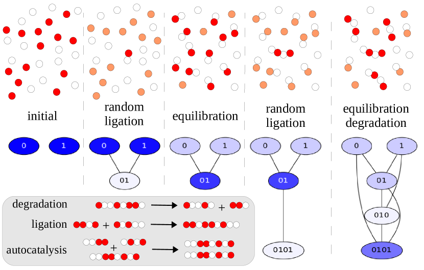
Figure 1: In the exact autocatalytic polymer model polymers made up of two types of monomers can degrade, ligate randomly or undergo autocatalytic replication (inlay). Strong autocatalysis and comparably rare random ligation promote the emergence of characteristic population structures (main image).

Several simple models have been developed to elucidate the prebiotic emergence and evolution of nucleic acid replicators. Most notably, random catalytic network models have been introduced to predict the emergence of autocatalytic cycles in pools of arbitrary molecules with random cross-catalytic activity Stadler et al. (1993); Hanel et al. (2005); Filisetti et al. (2012). More closely related to nucleic acids are catalytic polymer models, where the catalyzed polymer ligation reaction is modeled as concatenation of random strings Rasmussen (1985); Farmer et al. (1986); Kauffman (1986); Rasmussen et al. (1989); Bagley and Farmer (1991); Fernando et al. (2007); Hordijk and Steel (2012); Derr et al. (2012); Hordijk (2016). Most studies of polymer models concern themselves with the appearance of catalytic cycles when the catalytic activity of polymers is assigned either randomly or dependent on the sequence around the ligation site. Common conclusion of these studies is that random catalytic activity among a set of molecules is sufficient to promote the appearance of reflexively autocatalytic sets, i.e. groups of molecules that are able to jointly replicate themselves through cross-catalysis, see e.g. Refs. Kauffman (1986); Hanel et al. (2005); Hordijk and Steel (2014).

In this study, we take the appearance of catalysis and replication for granted, and raise the critical questions: do catalysis, replication, competition, cooperation, and selection indeed allow for the free exploration of the chemical sequence space or are some prebiotic evolutionary fates more common than others? If the latter, what is driving the evolution in such chemical networks? Ultimately, we want to better understand how prebiotic chemistry with reversible reactions can give rise to the emergence of history, i.e. can lead to a series of path dependent events, where the outcome of a past selection events impacts on what becomes accessible to evolution in the future.

In order to focus on these questions, we take a radical stance and study a polymer model in which autocatalysis is assumed to work perfectly for all molecular species. There are several reasons to do so. Firstly, if we believe chemical evolution to have evolved more and more effective self-replicators, it should be just as informative to understand the limiting case of perfect autocatalysis as it is to understand the limiting case of completely random chemistry. Secondly, by demanding perfect autocatalysis, we are able to derive closed analytic expressions for all involved molecular species. These allow us to scrutiny the reaction system with unprecedented analytic rigor, and we are able to align our simulation results with the analytic derivations.

We have previously reported on this model of self-replicating binary polymers where exact autocatalytic replication introduces a selection bias toward few specific replicator motifs and population structures Tanaka et al. (2014). Here, we present a full analysis of this system and several prebiotically motivated model variants.

In the remainder of the article, we give a detailed exposition of our simple binary polymer model with exact autocatalysis. We derive analytical results for the two important limiting cases of purely random as well as purely autocatalytic replication. We proceed by presenting simulation results of the prebiotically interesting case, where autocatalysis is dominent but augmented with relatively rare random ligation. For this scenario we reveal a strong inherent selection pressure toward repetitive sequence motifs. We suggest two non-exclusive explanations for the strong observed selection pressure, one that dominates the transient dynamics of the system, and one that acts upon equilibrated populations. We also analyze several variants of our model, including larger alphabet sizes, mutations, sequence complementarity, and non-replicating food species, before discussing the general implications of our findings.

II An exact autocatalytic binary polymer model

We study a system of self-replicating polymers made up of two types of monomers. Each polymer can (1) decompose into two substrands by hydrolysis of any of its bonds, (2) randomly ligate with another polymer to form a longer polymer, and (3) replicate itself autocatalytically by ligating two matching substrands. As an idealization, we assume that the rate constants of these reactions are constant and in particular independent of the sequence information of each polymer. As we are interested in the effect of catalysis, we assume that random ligations are comparatively rare.

The resulting system is a highly coupled molecular ecology, where replicating species compete for common resources and serve as each other’s reactants and degradation products. What will typically happen in such an ecology when starting from a pool of monomers?

To formalize this reaction system we first introduce some notation: let $\mathcal{A}=\left\{0,1\right\}$ be a binary alphabet. We denote the set of strings over $\mathcal{A}$ by $\mathcal{A}^{*}$, and we write $|k|$ for the length of string $k\in\mathcal{A}^{*}$. For $l,m\in\mathcal{A}^{*}$ we denote by $l.m$ the string obtained by concatenating $l$ and $m$.

We can now define the above reaction system formally, using the following three reaction rules:

$$l.m \xrightarrow{c_{0}}l+m$$ (1)

$$l+m \xrightarrow{c_{1}}l.m$$ (2)

$$l+m+l.m \xrightarrow{c_{2}}2\;l.m.$$ (3)

It has been observed experimentally, that non-enzymatic replicators suffer from product inhibition von Kiedrowski et al. (1991), where most potential templates are in their inactive double strand configuration, and thus cannot serve as replication templates. As a consequence, experimental replicators do not follow the exponential growth dynamics of simple autocatalysis and, in turn, promote coexistence of replicator species, rather than survival of only the fittest Szathmáry and Gladkih (1989); Fellermann and Rasmussen (2011). In our study, the implicit energy flow entering reaction (3) is assumed to separate the inactive and low energy double strand configuration of replicator strands and to transform them into their activated single strand configuration.

Since $\mathcal{A}^{*}$ is enumerable, we can take it as basis for an infinite dimensional state space: each state vector $x$ denotes a population within which every species $k\in\mathcal{A}^{*}$ spans one dimension and its associated coordinate $x_{k}\in\mathbb{R^{+}}$ specifies the concentration of the respective species. Standard dynamical systems analysis is complicated by the infinite dimensionality of this state space. Previous studies circumvented this difficulty by introducing a maximal strand length Bagley and Farmer (1991); Hordijk and Steel (2012) or focusing on very small monomer pools Wu and Higgs (2009); Derr et al. (2012). Here, we present a mathematical formalism that is able to deal with the infinite dimensionality for the most part analytically.

Assuming mass action kinetics, we can derive dimensionless reaction kinetic equations for the molar concentrations $x_{k}$ of species $k\in\mathcal{A}^{∗}$ as

$$\frac{\mathsf{d}x_{k}}{\mathsf{dt}} =\phantom{\alpha}\left(\sum_{\begin{subarray}{c}k.j=i\\ j.k=i\end{subarray}}x_{i}-\sum_{i.j=k}x_{k}\right)$$

$$+\alpha\left(\sum_{i.j=k}x_{i}x_{j}-\sum_{\begin{subarray}{c}k.j=i\\ j.k=i\end{subarray}}x_{j}x_{k}\right)$$

$$+\beta\left(\sum_{i.j=k}x_{i}x_{j}x_{k}-\sum_{\begin{subarray}{c}k.j=i\\ j.k=i\end{subarray}}x_{i}x_{j}x_{k}\right)\equiv f_{k}.$$ (4)

where we have chosen a time scale $t=c_{0}^{-1}$, and introduced the non-dimensional random ligation rate $\alpha=c_{1}/c_{0}$, and the non-dimensional autocatalytic ligation rate $\beta=c_{2}/c_{0}$. The above summations consider every pair of species $i$ and $j$ which satisfy $i.j=k$, and $k.j=i$ or $j.k=i$. Formally, the sum operators are defined by means of the indicator functions ($\mathbf{1}_{i.j=k}=1\text{ if }i.j=k\text{ else }0$) as follows:

$$\sum_{i.j=k} :=\sum_{i,j\in\mathcal{A}^{*}}\mathbf{1}_{i.j=k}$$ (5)

$$\sum_{\begin{subarray}{c}j.k=i\\ k.j=i\end{subarray}} :=\sum_{i,j\in\mathcal{A}^{*}}(\mathbf{1}_{j.k=i}+\mathbf{1}_{k.j=i})$$ (6)

Note that the second definition may involve an infinite sum and is only defined if the right-hand-side is defined. For finite size systems, which we consider in this article, the sum is always defined and allows us to write down the reaction equation system in a compact closed form without introducing any arbitrary truncation.

Equation (4) allows us to perform standard stationarity and stability analysis for the two limiting cases of purely random ligation as well as purely autocatalytic ligation.

II.1 Purely random and purely autocatalytic limit cases

In the absense of autocatalysis ($\beta=0$), the system approaches a stationary and stable equilibrium distribution, where the concentration of each replicator decays exponentially with its length:

$$\left(x_{\text{exp}}^{*}\right)_{k}=\frac{1}{\alpha}{\rm e}^{-b|k|},$$ (7)

which can be readily confirmed by inserting (7) into (4) for $\beta=0$. Here, $b$ is a constant determined by the boundary condition. Importantly, there is no selection for specific sequence patterns.

We will now show that this situation changes radically in the limit of purely autocatalytic ligation ($\alpha=0$). Firstly, since decomposition is now the only reaction that introduces novel species, any stationary state can only consist of initially present strands or their substrands. For any strand that is populated in the stationary state, all its substrands must be populated as well. This can be proven by contradiction: assume there exists a steady state $x^{*}$ with $x_{m}^{*}>0$ but $x_{k}^{*}=0$ for some $k.j=m$. From equation (4) it follows:

$$\left.\frac{\mathsf{d}x_{k}}{\mathsf{dt}}\right|_{x^{*}}=\sum_{\begin{subarray}{c}k.j=i\\ j.k=i\end{subarray}}x_{i}^{*}\geq x_{m}^{*}>0.$$ (8)

Since $f_{k}(x^{*})>0$, $x^{*}$ cannot have been a steady state. Thus, the assumption is false and species $k$ must be populated as well.

We call any strand that is not a substrand of any other strand in the population a “chief” and the set of its substrands its “clan”. An example of such a “chief-clan” structure is shown in figure 1. We denote the set of all chiefs of $x$ by $\partial\mathcal{A}^{\dagger}_{x}$ and the set of all clan members by $\mathcal{A}^{\dagger}_{x}$. Using this nomenclature, the stationary chiefs of the purely autocatalytic case are those substrands of initally present strands that survived decomposition and are not substrands of other surviving species.

Interestingly, under our assumption of exact replication (3), stationary species concentrations no longer decay exponentially with their length. Instead, any proper clan member is maintained at a constant concentration given by the replication rate constant $\beta$:

$$x^{*}_{k} =\begin{cases}\beta^{-1/2},&k\in\mathcal{A}^{\dagger}_{x}\backslash\partial\mathcal{A}^{\dagger}_{x}\\ 0,&k\not\in\mathcal{A}^{\dagger}_{x}.\end{cases}$$ (9)

This can again be readily confirmed by inserting (9) into (4) with $\alpha=0$.

Concentrations of chief species $m\in\partial\mathcal{A}^{\dagger}_{x}$ are unconstrained in the steady state, appart from what is determined by the boundary condition. This is so because the steady state condition for chiefs

$$\left.\frac{\mathsf{d}x_{m}}{\mathsf{dt}}\right|_{x^{*}}=-\sum_{i.j=m}x_{m}^{*}+\beta\sum_{i.j=m}x_{i}^{*}x_{j}^{*}x_{m}^{*}\\ =x_{m}^{*}\left(\beta\sum_{i.j=m}\beta^{-1}-\sum_{i.j=m}1\right)=0$$ (10)

is always fulfilled, independent of $x_{m}$.

To understand how stationary solutions respond to fluctuations, we derive the entries of the functional matrix:

$$\left.\frac{\partial f_{k}}{\partial\mathsf{x}_{l}}\right|_{x^{*}}=\sum_{\begin{subarray}{c}k.j=i\\ j.k=i\end{subarray}}\frac{\partial x_{i}}{\partial\mathsf{x}_{l}}-\sum_{i.j=k}\frac{\partial x_{k}}{\partial\mathsf{x}_{l}}\\ \quad+\beta\left(\sum_{i.j=k}\frac{\partial(x_{i}x_{j}x_{k})}{\partial\mathsf{x}_{l}}-\sum_{\begin{subarray}{c}k.j=i\\ j.k=i\end{subarray}}\frac{\partial(x_{i}x_{j}x_{k})}{\partial\mathsf{x}_{l}}\right)\\ =\left(\sum_{\begin{subarray}{c}j.l=k\\ l.j=k\end{subarray}}1-\sum_{\begin{subarray}{c}k.l=i\\ l.k=i\end{subarray}}1-\delta_{kl}\sum_{\begin{subarray}{c}k.j=i\\ j.k=i\end{subarray}}1\right),$$ (11)

where $\delta_{ij}=1$ if $i=j$ else 0 is the Kronecker symbol, and chief concentrations are assumed to be $\beta^{-1/2}$ for simplicity.

The equation simply expresses a detailed balance relation: increasing the amount of any clan species results in a flux to any species that uses the increased strand as prefix or suffix, while simultaneously introducing a flux away from all species needed as reactants for the formation of those longer species. Again, increasing the level of chief species ($l=m$) does not introduce any flux in the population structure. Notably, the stability of a stationary population is entirely determined by the topology of the reaction graph, not by the reaction rates.

To fully determine the stability of stationary solutions requires to solve for the eigenvalue spectrum of the functional matrix. The analytical treatment is complicated by the fact that the dimension of our system is formally infinite. We therefore resolve to numerically probing the eigenvalue spectrum of hundreds of different trial populations (see table 1). We find that the vast majority of stationary chief-clan structures have indeed no positive eigenvalues. Moreover, we find that the number of zero eigenvalues either equals the number of chiefs in the population or is one greater than that. Up to two of these zero eigenvalues result from mass conservation. The remaining ones express the fact that chief-clan structures with competing chiefs are connected by lines of linearly stable solutions. For example, in a population with competing chiefs $01$ and $10$ all populations that satisfy the constant solution $x_{0}=x_{1}=x^{*}$ are linearly stable, independent of how material is distributed among the chiefs.

Table 1: Stability of clans with different number of chiefs.

Clans with one chief
$|m|$	$P_{\rm sn}$	$P_{\rm ss}$	$P_{\rm u}$
2	1.00	0.00	0.00
4	1.00	0.00	0.00
6	0.40	0.60	0.00
8	0.20	0.80	0.00
10	0.07	0.93	0.00
12	0.02	0.98	0.00
14	0.01	0.99	0.00
16	0.00	1.00	0.00
18	0.00	1.00	0.00
Clans with two chiefs
$|m|$	$P_{\rm sn}$	$P_{\rm ss}$	$P_{\rm u}$
2	1.00	0.00	0.00
4	0.72	0.28	0.00
6	0.21	0.79	0.00
8	0.04	0.95	0.00
10	0.00	0.98	0.02
12	0.00	0.97	0.03
14	0.00	0.95	0.05
Clans with four chiefs
$|m|$	$P_{\rm sn}$	$P_{\rm ss}$	$P_{\rm u}$
2	1.00	0.00	0.00
4	0.82	0.18	0.00
6	0.19	0.81	0.00
8	0.01	0.99	0.00
10	0.00	0.99	0.01
12	0.00	0.99	0.01

$|m|$: the length of the chief(s), $P_{\rm sn}$: the probability to find stable nodes, $P_{\rm ss}$: the probability to find stable spirals, $P_{\rm u}$: the probability to find unstable stationary points. The number of sampling was $10^{4}$. Only combinations of chiefs that had the same number of “0” and “1” were sampled.

We remind that linear stability analysis only detects local stability and does not discriminate the relative stability of one solution over another. Moreover, our analysis does not consider boundary conditions, which might render some chief-clan structures less likely than others, if not outright impossible.

How many potential equilibrium solutions are there? We can roughly estimate the potential stable chief-clan structures as a function of the longest population member as follows: there are $2^{|m|}$ different chiefs of length $|m|$. If any of these chiefs can be either absent or present in the population, then there are $2^{2^{|m|}}$ different potential steady state populations. Despite the constraints of equation (9), there are super-exponentially many stable potential equilibrium populations. Already for strands as short as ten, this amounts to more than $10^{300}$ possible stationary chief-clan structures. One should bare in mind, however, that this estimation ignores the boundary condition imposed by the initial (and conserved) material amount.

So far our analysis has been based on molar concentrations. If material is sparse, however, it is more accurate to adopt the view that molecular species are present in discrete amounts. Under this view, the continuous equations (1)–(3) still describe the expected tendencies of the dynamic process, but with the difference that species can become extinct and disappear entirely, rather than being diluted to arbitrary small (but non-vanishing) concentrations. Under pure autocatalysis, this is especially relevant for chief species, as they are not constrained to potentially high equilibrium amounts. If chief species disappear as the result of random fluctuations, they become permanently extinct.

II.2 Combined random and autocatalytic ligation

We now study systems where both ligation reactions act in combination. In particular, we analyze how the system transitions from the exponential equilibrium solution to stable chief-clan structures when varying the ratio of the random and autocatalytic ligation rates.

To answer this question, we sample the stochastic process defined through (1)–(3) via exact stochastic simulation using a Gillespie algorithm. In order to tackle the dimensionality of the problem, the algorithm generates for the current state $x(t)$ a list of potential follow-up states on the fly and evaluates transition rates $r_{i}$ according to equation (4). For any finite size population, this transition list will also be finite.

Simulations are started from a monomer pool with $x_{0}(0)=x_{1}(0)=2100$, $\beta=10^{-4}$ and $\alpha$ varying from $10^{-7}$ to $10^{-3}$. Under sufficiently rare random ligation, we expect these settings to stabilize chief-clan structures up to length ten, and under only random ligation, an exponential distribution up to length eight. With the given $\beta$, in a population distributed according to (9), random and autocatalytic ligation would be equally likely for a random ligation rate constant $\alpha=\beta^{-1/2}=10^{-2}$.

After $t=1000$ time units, populations are compared to both equilibrium solutions (7) and (9) using the cosine similarities

$$s_{\text{exp}}=\frac{1}{\alpha}\frac{\sum_{k\in\mathcal{A}^{*}}x_{k}\mathrm{e}^{-b|k|}}{\left|x\right|\left|x_{\text{exp}}^{*}\right|}$$ (12)

and

$$s_{\text{ccs}}=\frac{\sum_{k\in\bar{\mathcal{A}_{x}}}x_{k}\beta^{-1/2}}{|\sum_{k\in\bar{\mathcal{A}_{x}}}x_{k}|\left|\sum_{k\in\bar{\mathcal{A}_{x}}}\beta^{-1/2}\right|}$$ (13)

where $\bar{\mathcal{A}_{x}}=\mathcal{A}^{\dagger}_{x}\backslash\partial\mathcal{A}^{\dagger}_{x}$. $s_{\text{exp}}$ the distance toward the corresponding exponential equilibrium and $s_{\text{ccs}}$ measures the distance to the smallest enclosing chief-clan structure, i.e. the smallest chief-clan structure that has a non-zero species count for any species that is present in the population.

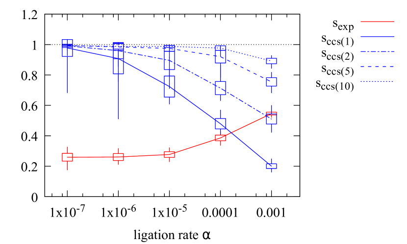
Figure 2: Cosine similarity between simulated population samples and ideal exponential distributions (red) and between the samples and their smallest enclosing chief-clan structure (blue), the latter for different threshold values. Species with occupancies below the threshold are not considered for the distance calculation.

Fig. 2 shows the transition from stable chief-clan structures into random distributions. With increasing random ligation rate $\alpha$, observed populations seize to resemble their original chief-clan structure. Visual inspection of the results revealed that these deviations are mainly caused by few random ligation products that are not numerous enough to establish their clan. When filtering ouf such outliers, we found that the remaining core populations resemble more closely their corresponding chief-clan structure, essentially until $\alpha$ reaches $10^{-2}$. At the same time, populations approach equilibrium distributions, because autocatalysis becomes too slow to generate chief-clan structures for the novel species created by random ligation. For high enough $\alpha$, deviation from the exponential equilibrium distribution is again mainly caused by rare long strands, whose expectation number from equation (7) is well below a single molecule.

These results indicate that chief-clan structures cannot develop above a critical random ligation rate less than $\beta^{-1/2}$. Approaching this critical threshold, chief-can structures become succeedingly obscured by random ligation products in low copy number.

II.3 Rare random ligation under strong autocatalysis

With the above insights we now concern ourselves with the prebiotically interesting parameter regime where comparatively rare random ligations occasionally introduce novel species into populations with strong autocatalytic replication. When starting from a pool of monomers, random ligation will create longer species that get amplified via autocatalytic replication and generate their clans via decomposition. We expect this process to generate chief-clan structures satisfying equation (9) of a size that is just able to accommodate the overall amount of material.

Our question now becomes: does autocatalytic replication with rare random ligation generate all of the overwhelmingly many potential chief-clan structures, or is there some reason for some chief-clan structure to be more prominent than others?

Using the results of 1000 simulation runs (simulated until $t=100$), we perform single linkage hierarchical clustering based on cosine distance

$$d(x,x^{\prime})=1-\frac{\sum_{k\in\mathcal{A}^{*}}x_{k}x_{k}^{\prime}}{|x||x^{\prime}|}.$$ (14)

We find that about 75% of the simulation results concentrate in six clusters with characteristic population structures, shown in figure 3. This is a very strong selection pressure, given that all our kinetic equations are sequence agnostic—especially under the light of the results of the previous discussion.

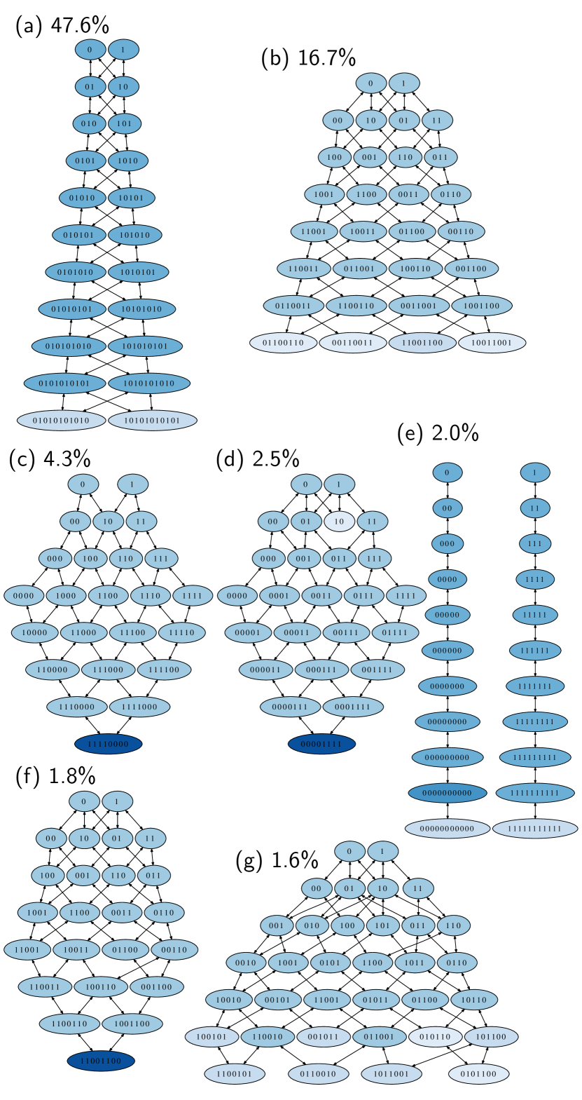
Figure 3: The result of hierarchical clustering for 1000 populations produced by simulation; Named: (a) bootlace, (b) pinecone1, (c) pinecone2, (d) pinecone2, (e) two-towers, (f) pinecone1. Cluster (g) has no name and there are many similar structures. Note that (b) and (f), and, (c) and (d) belong to the same symmetry. These seven clusters occupy 76.5% of all the population produced. Species having less than 10% of the constant solution are omitted. Simulations were run with $\alpha=10^{-10}$, $\beta=10^{-7}$, and $x_{0}(0)=x_{1}(0)=200\,000$.

Interestingly, the selected populations have very few chiefs composed of short repeating sequence motifs such as 01 in cluster 3(a) (bootlace), 0011 in cluster 3(b) and (f) (pinecone1), 00001111 and 11110000 in cluster 3(c) and (d) (pinecone2). In about 2% of the simulation runs, we even observe complete demixing of the monomers into homopolymers composed exclusively of 0’s and 1’s respectively (cluster 3(e), twotowers).

We also observe that some clusters exhibit an “inverted” population structure where chiefs are more populated than other clan members (3(c), (d), and (f)). This is due to the boundary condition where the total material amount is too low to maintain a longer chief but too high for the chief concentration to be comparable to the equilibrium value. As a consequence, the highly populated chief will more likely create—via random ligation—species outside its clan structure, which either die out or cause the whole population to transition into another structure. Indeed, we have observed in simulation that these metastable structures exhibit stronger random fluctuations and potentially transition into completely distinct chief-clan structures Tanaka et al. (2014).

We emphasize that the stochastic simulation results are rather unexpected, if not even in apparent contradiction to the results of the linear stability analysis derived above. If linear stability theory allows for almost any chief-clan structure to be (at least meta-)stable, how come that stochastic simulation exhibits such a strong bias toward selecting very few and very regular population structures? What constitutes this “survival of the dullest”?

III Mechanisms of structure selection

We now propose two possible explanations for the symmetry breakdown in this replicator ecology: On the one hand, we identify a selection bias in the transient process of creating equilibrated, non-inverted chief-clan structures. On the other hand, we identify a selection bias in the steady state dynamics of an established equilibrated population. Both selection biases steer the system toward highly repetitive sequence patterns, and we hypothesize that both of them are responsible for the strong selection observed in stochastic simulation.

III.1 Selection in locally equilibrated populations

We first discuss the equilibrium scenario. Consider an equilibrated population structure that satisfies (9) and comprises two chiefs $a$ and $b$. The clans of these chiefs always overlap (because monomers take part in all clans) and the overlap forms a pool of common resources for the two clan structures to compete over. As in the end of the previous section, we assume random ligations to be sufficiently rare and use equilibrated chief-clan structures as initial conditions.

It is illustrative to first investigate a minimal system of four species, where two chiefs $01$ and $10$ compete over the shared resources $0$ and $1$. We know from the above that mass conservation of the two monomers fixes this system on a two dimensional plane, which features a continuous line of marginally stable steady states due to condition (9). The line connects the two boundary states, formed by populations with only one surviving chief species.

In a stochastic treatment of this system, the line of connected equilibria, translates into a drift term that vanishes for equilibrium solutions. Unlike in the deterministic treatment, random fluctuations can now redistribute material along the line of marginal steady states with virtually no deviation from equilibrium. The two boundary states are absorbing boundaries, as the walk terminates if one of the competing chiefs becomes extinct (and cannot be repopulated in the absense of random ligations).

Interestingly, diffusion of the random process also becomes position dependent: randomly converting a single chief molecule from one species to the other requires the abundance of both chief species, one entering as reactant to be degraded, the other as catalyst to enhace its own ligation. Diffusion is therefore the highest when the product of the two chiefs is maximized and goes toward zero when approaching the boundaries, where either of the two species becomes sparse.

In the appendix, we develop a one dimensional random walk, constrained to the line of connected steady states, that approximates the two dimensional case. For this approximation, we are able to analytically derive a Fokker-Planck equation that features zero drift and position dependent diffusion:

$$\frac{\partial}{\partial\mathsf{t}}P(x_{01},t) \approx\frac{\partial^{2}}{\partial\mathsf{x}_{01}^{2}}\left[D(x_{01})P(x_{01},t)\right]$$ (15)

where $D(x)=\frac{x_{01}x_{10}-1}{x_{01}+x_{10}}$.

The parabolic diffusion term has a remarkable effect on the first hitting time, i.e. the typical time of chief coexistence. Because diffusion is higher in the center of the manifold (where both chiefs are populated about evenly) the system is more prone to leave this state and move toward states of lower diffusion. This diffusion induced effective drift drives the system toward regions where one chief outnumbers the other. The average time for the system to reach one of the absorbing states is therefore orders of magnitude shorter than for a random walk process with comparable, but constant diffusion. Figure 13 of the appendix compares the cumulative probabilty functions of the hitting time distributions for the original two dimensional system, our one dimensional approximation, and a random walk process with constant diffsuion.

Perheaps contrary to expectations raised by the previous linear stability results, we now see that there is a natural tendency for minority species to be driven into extinction. This effective drift is ultimately induced by position dependent diffusion along the line of competing chief populations.

Note that this effective drift can only be observed among chiefs that can absorb all the material of their competitor: otherwise, both chiefs can survive. For example, two chiefs $010$ and $101$ can coexist because neither can absorb all the material of the other. Yet, deviations in the chief-clan structure from the constant solution can sometimes absorb a chief with different material than its competitor, as we discuss now.

Figure 4 shows how a short chief, $00$, can be driven into extinction as the result of competion with longer chiefs: simulations are initialized with equilibrated bootlace structures of varying length, plus $00$, and measure the probability of survival of the shorter chief after 1000 time units as a function of its initial concentration for varying length of the longer chief. In this case, chiefs in a bootlace structure, such as $0101$, cannot absorb all the material of $00$, but the short chief can nevertheless be absorbed by fluctuations of the chief-clan structure, which in turn deviates from the exact solution 9. The simulation shows the clear tendency of extinction of shorter clans in competition.

(a)

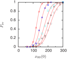
(b)

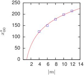
Figure 4: (a) Probability of survival, $P_{\rm sv}$, after $t=1000$ for 00 coexisting with a bootlace structure (figure 1) with different chief length, depending on its initial concentration $x_{00}(0)$. The chief length are: $|m|=4$ ($\times$), $|m|=6$ ($\ast$), $|m|=8$ ($\square$), $|m|=10$ ($\diamond$), and $|m|=12$ ($\circ$). The solid curves are fitted error functions. (b) The threshold value, $x_{00}^{\ast}$, where $P_{sv}=0.5$ against the chief length $|m|$. The solid curve is a fitted logarithmic function.

While the above reveals the source of competition and extinction in our model, and indicates that simulations should generate populations with few chiefs, it does not explain why the dynamics select those particular chiefs that feature simple repetitive motifs.

An answer to this question lies in the way perturbations are distributed among competing clans, as shown schematically in figure 5: When species in the overlap of competing clans are perturbed through random decomposition of longer strands, detailed balance causes an opposing flow from the perturbed species toward longer strands. This outflow can be partitioned into three components: material flowing into species belonging exclusively to clan $A$, clan $B$, or their overlap $C$:

$$\frac{\partial f^{A\cup B\cup C}_{l}}{\partial\mathsf{x}_{l}}=\frac{\partial f_{l}}{\partial\mathsf{x}_{l}}.$$ (16)

where we have introduced the “partial” flow $\frac{\partial f^{A}_{l}}{\partial\mathsf{x}_{l}}$ from $l$ into the species in $A$:

$$\left.\frac{\partial f^{A}_{l}}{\partial\mathsf{x}_{l}}\right|_{x^{*}}=-\left(\sum_{\begin{subarray}{c}l.j\in A\\ j.l\in A\end{subarray}}1+\sum_{l.l\in A}2\right)\approx-\sum_{\begin{subarray}{c}l.j\in A\\ j.l\in A\end{subarray}}1.$$ (17)

Thus, the flow into $A$ ($B$) scales with the number of strands in $A$ ($B$) that have the perturbed strand as their prefix or suffix. Since regular chiefs can form longer strands with more repetitive sequences than irregular chiefs, we expect regular chiefs to outperform irregular ones in this competition.

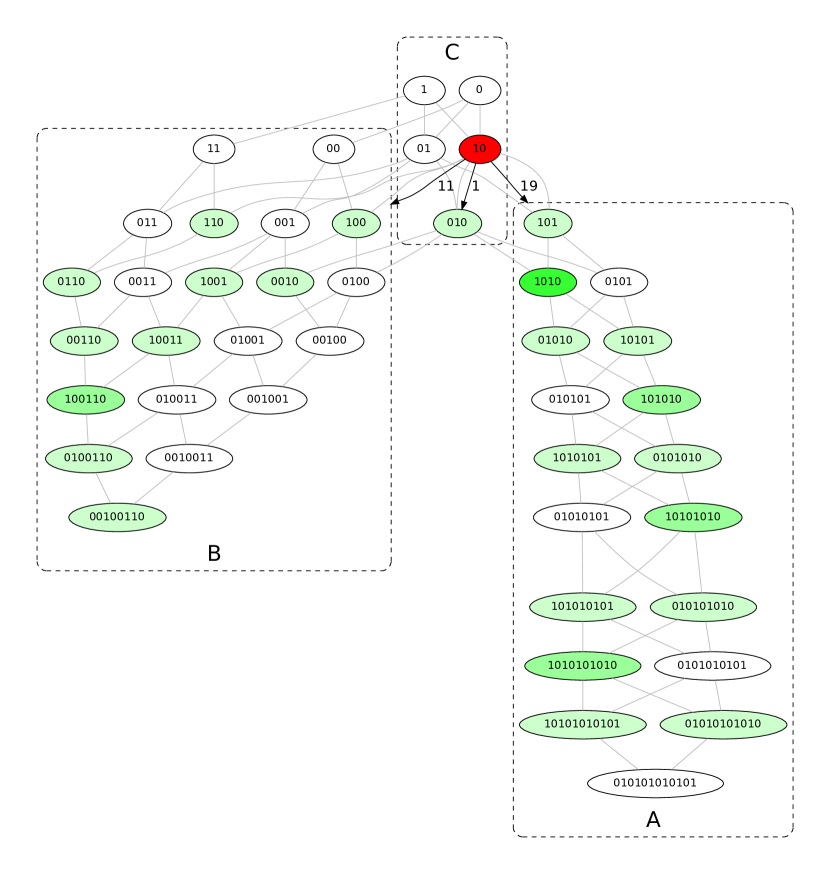
Figure 5: Visualization of the “partial flows” when a population in equilibrium state $x^{*}$ is perturbed by adding $\Delta x$ to species $l=10$. In the case shown, ${{\rm d}f_{l}}/{{\rm d}x_{l}}=-31$ (red). This flow is distributed such that $-{{\rm d}f^{A}_{l}}/{{\rm d}x_{l}}=19$ go into clan $A$, $-{{\rm d}f^{B}_{l}}/{{\rm d}x_{l}}=11$ go into clan $B$, and $-{{\rm d}f^{C}_{l}}/{{\rm d}x_{l}}=1$ remain in the overlap $C$. Green nodes show the recipients of material where light green corresponds to $1$, medium green to $2$, and dark green to $4$.

Summary

In equilibrium strands with high population numbers outcompete low populated strings in competition for resources and this makes it difficult for randomly created chiefs to survive. In some cases this process can be described by a Fokker-Planck equation, which expresses a position dependent diffusion. Further, long clans can absorb material faster than short clans because they offer more reaction pathways to absorb fluctuations (due to an increased number of prefix/suffix matches). With a given amount of material, regular chiefs can form longer clans than irregular ones.

III.2 Selection far from equilibrium

We now discuss the transient dynamics of a typical process of structure generation that starts from a pool of monomers, where—as before—random ligation is small enough for the system to locally equilibrate after each random ligation event. Thus, after spontaneous formation of an intermediate chief through random ligation, the new chief will accumulate material via autocatalysis in order to satisfy the equilibrium condition (9). The result is an inverted population structure where chief species accumulate the majority of the material. Therefore, the next ligation is more likely to happen among two chiefs than among any other species in the population—thus creating a strand with repeated sequence patterns Tanaka et al. (2014). Irregular chiefs, on the other hand, require additional substrands to be formed from now less abundant clan members. The process repeats until chief concentrations become lower than the equilibrium solution, at which point there is no surplus material to grow longer strands.

The above verbal argument can be refined into a quantitative estimation of selection likelihoods: assuming that populations grow by irreversible random ligation and subsequent equilibration, the likelihood to obtain one population from a previous one via a single ligation event is proportional to the equilibrium abundance of the reactants, which is largely determined by the equilibrium condition (9). Assuming that the surplus material is evenly distributed among chief species, we can calculate the probability to obtain any final population from the initial condition by multiplying the conditional probabilities of ligations along each ligation pathway that can lead to the final population in question. However, because of the double exponential scaling of potential chief-clan structures as a function of chief length, the reaction system leads to a combinatorial explosion that fastly exceeds computing resources. Justified by equation (17) and the results of figure 4, we introduce the additional assumption that a new chief can only form in a population if it is at least as long as any existing chief. With this additional assumption, the combinatorial problem can be tackled.

We systematically perform these likelihood estimations for different initial monomer amounts and estimate the 90% most likely ligation pathways. The resulting population structures are classified according to their sequence motifs and compared to the results of stochastic simulations for selected pool sizes. The computed likelihoods—shown in figure 6—are generally in good agreement with the simulations.

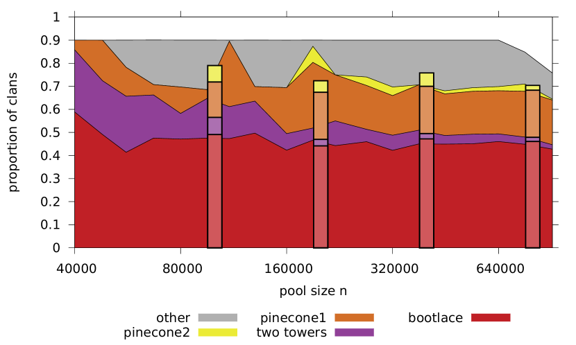
Figure 6: Estimated likelihood to form populations of strands with certain motifs as a function of the monomer pool size with balanced monomer compositions. Note the exponential scale of the $x$ axis. Overlaid bar charts show results of full stochastic simulations for various system sizes. See text for details.

Summary

During the transient equilibration moves most material into chiefs. If there is a single chief, it will most likely react with itself to create the next chief (scenario $01+01\to 0101$). The key here are inverted population structures Tanaka et al. (2014) where most material is in the chief species. To make irregular sequences during the transient, distinct building blocks are needed. If one chief has absorbed the material, there is less material for the other chief, thus reducing the propensity of forming the irregular chief (scenario $10+0\to 100$). Again most material is in the chief. To make a particular irregular chief during the transient, the two substrings have to ligate in correct order (scenario $10+0\to 100$ vs. $0+10\to 010$), so the symmetry of the reaction network plays as only one of two possible reactions produce a non-repetitive sequence. Finally, regular chiefs require the build-up of fewer intermediate species, i.e. 01010101 requires only 01 and 0101, whereas 01110001 would require 01, 11, 00, 01, 0111 and 0001 or a similar number of other intermediates.

III.3 Distinguishing the alternative selection mechanisms

We have presented two alternative driving mechanisms that might explain the selection of few chiefs with short repetitive motifs. Which of these mechanisms is responsible for the results presented in figures 2 and 3?

In order to discriminate the two selection mechanisms, we perform numerical simulations and measure—over the course of time—the number of species and chiefs, an activity measure $A$ that measures the surplus of material in chief species through the definition

$$A(x)=\sum_{x_{i}\in\partial\mathcal{A}^{\dagger}_{x}}\left(\frac{x_{i}}{x^{*}}\right)^{2}\left(\frac{x_{i}}{x^{*}}-1\right)^{2},$$ (18)

as well as the cosine similarity $s_{\text{ccs}}$ of the population with the smallest enclosing chief-clan structure.

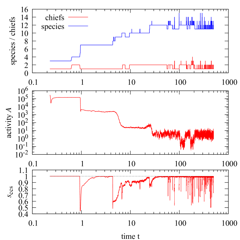
Figure 7: Typical development of chief-clan structures (here bootlace) under rare random ligation. Parameters are chosen as in figure 2 with $\alpha=10^{-7}$. Graphs show the number of species and chiefs (top), an activity that measures how “inverted” the population is (middle), and the distance to the smallest enclosing chief-clan structure (bottom). See text for details.

Figure 7 shows exemplary results for the formation of a bootlace structure under the parameters of figure 2 with $\alpha=10^{-7}$. The stepwise elongation of the bootlace structure is reflected by a steady increase in species count, but a non-growing number of either one or two chiefs. While the structure grows, the activity generally decreases, until it levels off around $t=30$ where the structure is fully established. Each formation of new chiefs in the structure leads to a temporary decrease in the otherwise maximal cosine similarity to the corresponding chief-clan structure. This decrease in similarity is caused by the temporarily high population count of the previous chief, which now violates the constant solution. Similarity is regained with the autocatalytic flow of matter into the newly formed chief, and is accompanied by a decrease in activity.

These observations indicate that the selection of the bootlace structure occurs from the onset and is caused by the far-from-equilibrium selection mechanism that is active during the transient period. Yet, once the structure is fully developed around $t=30$, the equilibrium selection mechanism stabilizes the developed population and prevents the occurence of new chiefs. As a result, fluctuations in species and chief numbers, activity, and similarity are short-lived.

Visual inspection of several dozens simulation runs confirms this general behavior independent of the nature of selected structure. The lower the random ligation rate $\alpha$ the more prominent the far-from-equilibrium selection. For the parameters chosen (c.f. figure 2), clear chief-clan structures form and remain stable for $\alpha$ between $10^{-7}$ and $10^{-6}$. For $\alpha=10^{-5}$, the dynamics still yield a transient selection, but the selected chief-clan structures is no longer maintained in equilibrium, as random ligations become too common. Finally, for $\alpha=10^{-4}$ and above, stable chief-clan structures can no longer form (at least without applying a threshold for the structure identification).

IV Model variants

We now present several variations of our original reaction system to demonstrate that the reported selection pressure is structurally robust and can be observed in similar replicator systems that more closely resemble the chemistry of nucleic acid replicators.

IV.1 Increased alphabet size

Alphabet size has a significant impact on the selected population structures. Here we show populations produced from a pool of four types of monomers ($\mathcal{A}=\left\{0,1,2,3\right\}$). Although introducing new monomer types makes the system more complex quickly, the selection of chief-clan structures does happen as shown in figure 8. The six largest clusters contain about 25% of all the populations produced. They all feature permutations of 0123 as motifs. They are thus a counterpart of the bootlace structure with motif 01. As in the case of a binary alphabet, symmetry is broken at the level of dimers and propagates from there through the population structure. From the seventh cluster onwards [figure 8(b)], structures lose order and become more irregular.

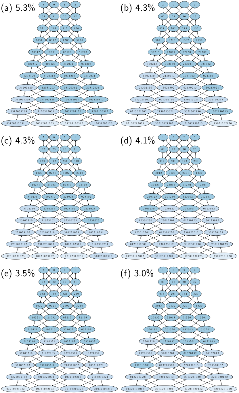
Figure 8: The structures produced from simulations with $\mathcal{A}=\left\{0,1,2,3\right\}$. They all belong to the same motif, $\ldots 0123\ldots$, and its permutations. All six permutations of the motif appear in simulation, occupying in total 25% of all populations. After the 6th cluster, the structure becomes random. The parameters used: $\alpha=10^{-10},\ \beta=10^{-6}$ with $2\times 10^{5}$ of 0, 1, 2, and 3. The hierarchical clustering was stopped when 30% of populations are included into the largest 10 clusters. Species less than 30% of the constant solution are omitted.

IV.2 Mutations

Evolution arises from variation and selection. In our basic model, variation is entirely due to random ligation. It is interesting to see how the reported sequence selection in our model is affected when potential mutation opens an additional channel for variation. To this end, point mutations are introduced as a reaction:

$$l^{\prime}+m^{\prime}+l.m \xrightarrow{\;\;c_{3}|l.m|\;\;}l^{\prime}.m^{\prime}+l.m$$ (19)

where $l^{\prime}.m^{\prime}$ is one bit different from $l.m$, and $c_{3}/c_{2}=10^{-4}$.

Figure 9 shows the largest and second largest clusters found in simulation. The largest cluster [figure 9(a)], occupying 34% of all populations, is based on the bootlace structure [figure 3(a)], whereas the second largest cluster [figure 9(b)], occupying 10%, is based on the pinecone1 structure [figure 3(b)], judging from the tetramer and pentamer sequence motifs. In figure 9(a), despite the fairly large mutation rate, perturbations arising from point mutations only produce short additional chiefs, and the bootlace structure remains unperturbed in its longer sequences. On the other hand, the distortion in figure 9(b) is significant. Actually, all the species shorter than trimers appear. This indicates that the robustness against mutations depends on the population structure, which likely connects to the different stabilities of the structures.

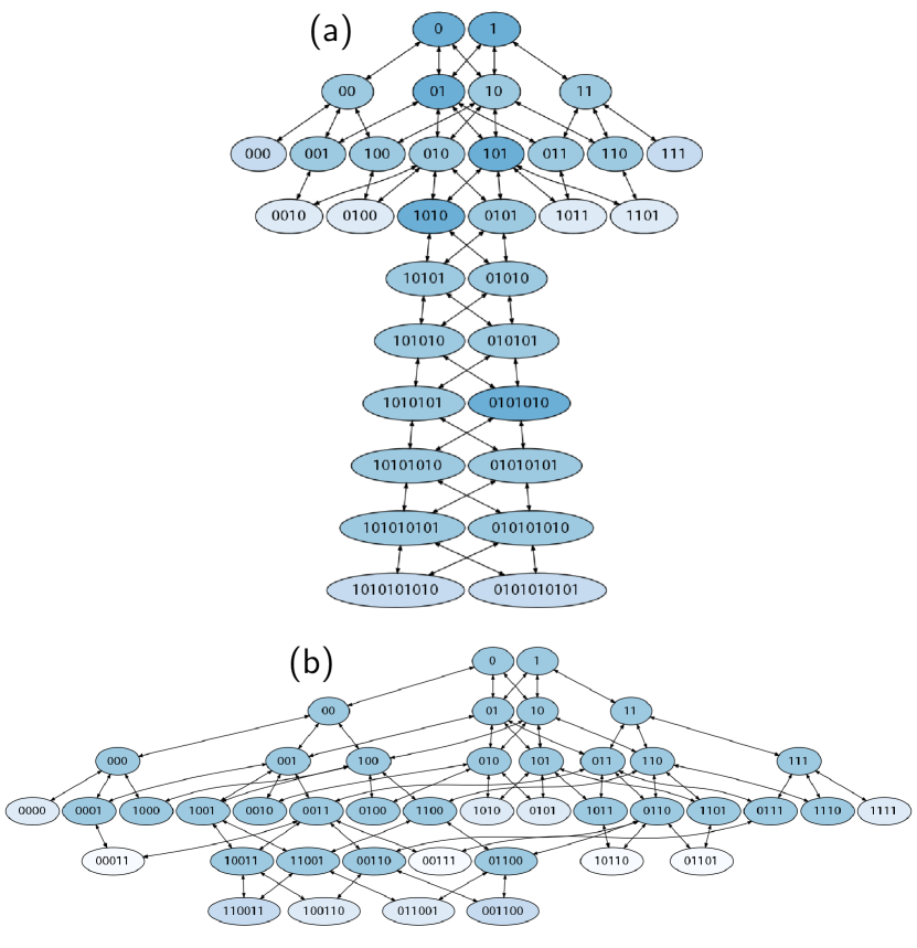
Figure 9: The structures produced from simulations with mutation. Bootlace, (a), is more robust against mutation than pinecone1, (b), which is disturbed significantly. The occupancy is 34% and 10% for bootlace and pinecone1, respectively, in 697 runs. The parameters used: $\alpha=10^{-10},\ \beta=10^{-7}$, $c_{3}=10^{-11}$ with $2\times 10^{5}$ of 0 and 1.

IV.3 Sequence complementarity

Sequence complementary hybridization is a characteristic feature of template directed nucleic acid replication. We introduce sequence complementarity into our model by defining a complementarity operator $\overline{\vphantom{t}\cdot}:\mathcal{A}^{*}\rightarrow\mathcal{A}^{*}$ recursively as follows:

$$\overline{0} =1$$ (20)

$$\overline{1} =0$$ (21)

$$\overline{l.m} =\overline{l}.\overline{\vphantom{l}m}$$ (22)

This allows us to replace the original template directed ligation reaction (3) by its sequence-complementary counterpart:

$$l+m+\overline{l.m}\xrightarrow{\;\;c_{2}\;\;}l.m+\overline{l.m}.$$ (23)

Figure 10 shows a result of hierarchical clustering out of 1000 runs. The seven clusters shown in figure 10 occupy about 70% of all the clusters produced. This value is slightly smaller than the case in figure 3, but still significant fraction, indicating a strong dynamical selection. On the other hand, the occupation of each cluster becomes different from the case in figure 3. The bootlace structure, for example, is still a biggest cluster, but it occupies only about 11% in comparison with 48% shown in figure 3. Pinecone1 [figure 10(b) and (c)] and two-towers [figure 10(d)] increase their occupancy. Three new clusters [figure 10(e), (f), and (g)] appear as replacing the bootlace’s occupancy. One also notices that all the structures shown are symmetric about the center axis, reflecting the complementarity.

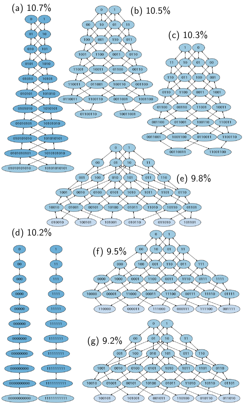
Figure 10: The structures produced by sequence complementary autocatalysis. The parameters used: $\alpha=10^{-10},\ \beta=10^{-7}$ with $2\times 10^{5}$ of 0 and 1. These seven clusters occupy about 70% of all the populations produced.

IV.4 Existence of inert food species

Several previous studies assume the existence of food species Hordijk and Steel (2012); Derr et al. (2012) that cannot be produced by autocatalysis and thus have to be present in the system in the beginning or have to be fed continuously into the system. In our basic model, monomers are the only food species. We now analyze a variant where any species up to a certain length $l_{\rm food}$ are food species that cannot undergo autocatalysis. As a consequence, the system does not have to satisfy the constant solution (9).

To examine the effect of food species, we conducted a stability test. First, a bootlace structure including food species, with two chiefs of length $|m|$ is constructed assuming that all species has the same concentration given by the constant solution. Then the system is equilibrated. Figure 11 shows a diagram indicating whether the bootlace structure is stable or not, depending on $|m|$ and $l_{\rm food}$. It can be seen that the structure is stable if the length of the chief is long enough. The neccesary length stabilizing the bootlace is roughly linearly proportional to $l_{\rm food}$.

Figure 12 shows a distribution of species in equlibrium. Crosses show a distorted bootlace structure, where the distribution of food species decreases exponentially. For autocatalytic species, the constant solution is approximately recovered with slightly larger values.

If we start simulations from a pool of monomers, monomers must spontaneously ligate to become longer than $l_{\rm food}$ to initiate autocatalytic reactions. It is unlikely then, that autocatalytic species appear spontaneously unless the concentration of monomers is extremely high. Circles in figure 12 show the distribution when the simulation is started with the same amount of monomers as above, but without a pre-constructed bootlace structure (crosses in figure 12). Only dimers appear in this case. Therefore, it is unlikely, if not impossible, for this system to achieve spontaneously autocatalytic species and the resulting distribution maintained by autocatalysis.

This barrier between autocatalytic and non-autotacalytic states depends strongly on the size of food species. The longer the food species, the higher the barrier. This observation is important, for example, to a real chemistry or origin-of-life scenarios. The available monomer concentration determines how long the food species is tolerated to achieve an autocatalytically maintained state.

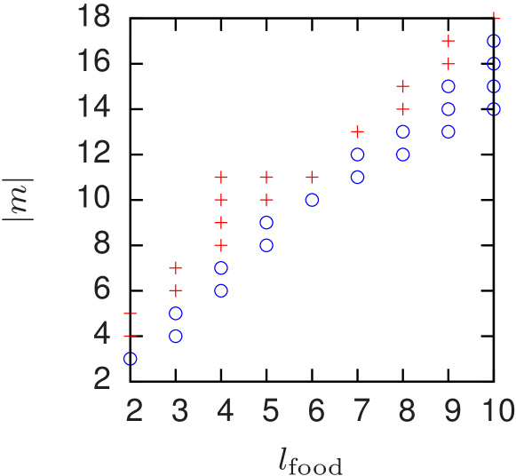
Figure 11: A stability diagram of the bootlace structures with their chief length $|m|$ against the maximum length of food species, $l_{\rm food}$. Crosses and circles represent where they are stable and unstable, respectively.

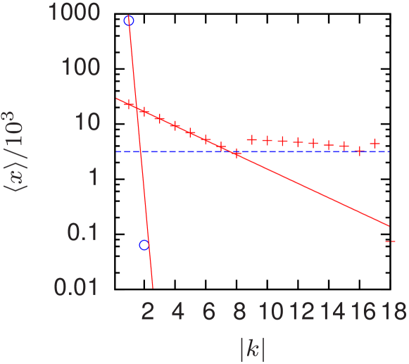
Figure 12: The averaged distribution of species, $\langle x\rangle$, depending on their length, $|k|$ when $l_{\rm food}=8$. Crosses represent a case starting from a pre-built bootlace structure, whereas circles represent a case starting from a pool of monomers. Solid lines represent exponential functions. Dashed line is the constant solution, $\beta^{-1/2}$.

V Discussion

We have presented a simple model of binary self-replicating polymers, in which exact autocatalysis gives rise to the formation of characteristic chief-clan structures, where the sequence information of the longest replicators completely determines the population distribution of the molecular ecosystem. When starting from a pool of monomers, only few, highly regular sequence patterns are selected by the dynamics.

We attribute this selection for repetitive sequences to stems in part from reaction symmetries and in part from a transient concentration of material in the long sequences. Due to the reaction conditions during the transient, most material is concentrated in the long sequences, the chiefs. In the transient formation of the longer sequences, mainly from the abundant chiefs,repetitive sequences both have more and shorter reaction pathways due to their symmetries. This is true both in the ligation of shorter sequences into longer sequences and in the breakdown of longer sequences into shorter sequences. These are the reasons why the production of repetitive sequences are favoured in such systems.

Notably, this dynamical selection is intrinsic to our model and does not require an a priori fitness function. This is important for the study of, for example, prebiotic evolution and origins of life Joyce (1984); Breaker and Joyce (1994); Vaidya et al. (2012), as well as protocell research Szostack et al. (2001); Fellermann (2011); Rasmussen et al. (2016), since it implies that the selection occurs by means of both environmental as well as internal factors. This aspect was not elucidated by previous studies where selection was either induced by means of an external fitness function or by assigning randomly attributed catalysis rates.

It is commonly understood that random fluctuations are mostly significant in systems with small molecular copy numbers and that, in the limit of large numbers, results of stochastic simulations typically approach expectation values that can be obtained from equivalent deterministic models. The situation is radically different in the system presented in this study: firstly, autocatalytic replication amplifies small random fluctuations in the transient, which ultimately determines the fate of entire populations on the system level; and secondly, steady state population numbers are only determined by reaction constants, but not by the total material concentration. Increasing the total monomer concentration will not increase the concentration of molecular species in steady state. Instead, the system will accommodate for the additional material by generating larger polymers, up to a length where material becomes sparse and thus remains susceptible to copy number fluctuations.

Although our exact findings have been derived by analyzing a specific reaction system (exact autocatalysis), we hypothesize that many of our general results also hold for similar binary polymer models, for example those employing sequence dependent replication rates Derr et al. (2012), random cross-catalysis Bagley and Farmer (1991), or material flow.

Namely, if studied under conditions where the analysis of our work applies (sufficiently high molecule numbers, dominant catalysis over random ligation, and relatively constant environment), any polymer chemistry is expected to approach some equilibrium distribution. The phase space profile of these equilibrium states will dictate which populations are stable and how matter is distributed among their members. If the kinetics of the polymer chemistry allows for multiple equilibria, selection is likely to occur. Either because these are isolated stable states and an initial population has to commit to one or the other; or because a smaller set of stable states is selected by noise induced drift, as encountered in the chemistry studied in this article. For example, Bagley et al. Bagley and Farmer (1991) report the emergence of “concentration landscapes” in randomly catalyzing polymer networks, which we can now identify as equivalents to chief-clan structures.

As long as selected populations introduce novel species that provide resources and catalysts for higher units of selection (i.e. longer polymers of a net-catalyzing set), the chemistry meets in principle the conditions for continued selection dynamics during a transient that starts from monomers or short oligomers. In the model system discussed in this article, continued selection is particularly prominent, since every newly created species is an auto-catalyst. Continued selection is expected to stall once the chemistry does not introduce novel resources or novel catalysts. For example, if the chemistry allowed for overhangs around a ligation window, we expect the symmetry breakdown to stall, once a suitable ligation site has emerged.

In contrast, we expect that the particular repetitive sequence motifs that we report here stem from symmetries in the reaction graph of exact autocatalysis and are likely not prominent in random catalytic chemistries.

The investigation of related chemistries employing sequence dependent and randomly assigned catalysis is left for future research.

Appendix A Fokker Planck derivation

We study the minimal competing system with four species, where two competing chiefs $01$ and $10$ compete over resources $0$ and $1$. Mass conservation maintains the dynamics on a two dimensional manifold, essentially $x_{01}$ and $x_{10}$ ($x_{0}=x_{1}$ can then be infered).

For brevity, we introduce the notation $X=01,Y=10$, with concentrations $x=x_{01},y=x_{10},z=x+y$, and indistrimnately refer to monomers by $A$ with concentration $a=x_{0}=x_{1}$.

Motivated by the observation that there is a line of steady state solutions (any combination of $x$ and $y$ that fulfills $a=\beta^{1/2}$) that are all of marginal stability (zero eigenvalues), we introduce a simplification that constrains the system to maintain equilibrium by only distributing material among chiefs.

To achieve this, we construct a constrained stochastic process, where no two degradations nor two ligations can follow each other without an intermediate event of the other type. Each net degradation-ligation event thus maintains the initial distance from the equilibrum line.

Technically, we introduce a stochastic net process with two Markovian degradation reactions, and two delayed time ligation reactions whose rates $\beta$ are functions of the time $t-t^{\prime}$ since the last degradation event. With

$$\int_{t^{\prime}}^{\infty}\beta(t-t^{\prime})dt=\beta,$$ (24)

we ensure that the original ligation rate is maintained in the long term. Informally, the constrained process can be written as

$$X \xrightarrow{1}2A\xrightarrow{\beta(t-t^{\prime})x}X$$ (25)

$$X \xrightarrow{1}2A\xrightarrow{\beta(t-t^{\prime})y}Y$$ (26)

$$Y \xrightarrow{1}2A\xrightarrow{\beta(t-t^{\prime})x}X$$ (27)

$$Y \xrightarrow{1}2A\xrightarrow{\beta(t-t^{\prime})y}Y.$$ (28)

We now let

$$\beta(t-^{\prime}t)\rightarrow\beta\delta_{t-t^{\prime}}$$ (29)

approach a Dirac distribution, so that ligation follows degradation immediately.

Degradation events occur as previously with rate constant 1, but only a certain fraction (e.g. $y/(x+y)$ for equation (26)) lead to an actual change in the system state. The net conversion rates are therefore the degradation rate (having been set to one per unit time in the dimensionless system) times the probability to lead to a system change. The net process therefore reads:

$$X\xrightarrow{(z-x)/z}Y$$ (30)

$$Y\xrightarrow{x/z}X$$ (31)

Note that the total propensity of this net process, $(z-x)/z+x/z=z$, equals the total propensity of degradations in the original process.

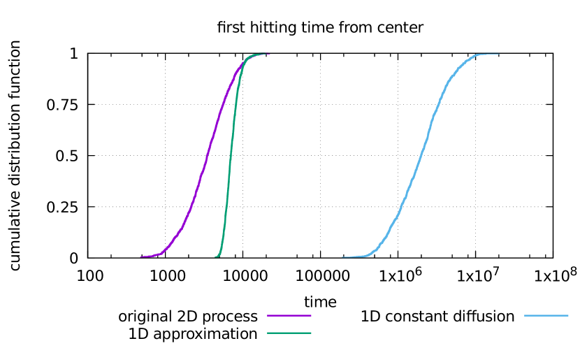
Figure 13: Cumulative hitting time distributions of different random walks starting in the inital state $x(0)=\frac{z}{2}=\frac{x^{*}}{2}$ for $z=\sqrt{10^{7}}$. Distribution functions have been obtained from 1000 numerical samples for each of purple: the original 2D process defined by equations (1) and (3), green: our 1D approximation of equation (30), and blue: a random walk with constant diffusion for reference.

To compare the quality of this approximation, we sampled 1000 instantiations of the original 2D process and of our 1D simplification and compare the cumulative probability distributions of first hitting times for walks that start at $x(0)=\frac{z}{2}$ and reach one of the absorbing bundaries $0$ or $z$. Results are shown in figure 13.

The results reveal that the 1D approximation generates hitting time distributions with the same general shape than the original process, but overestimates typical hitting times – that is, the unconstrained process typically terminates faster than the constrained process. The approximation is more accurate for late hitting times, and approaches the original hitting time distrubtion.

Figure 13 also reveals that both the original and the constrained process complete orders of magnitude faster than a random walk where $X$ transforms into $Y$ and vice versa with constant rate $z$.

We now derive the Master and Fokker Planck equations for the stochastic process (30)—(31). Since mass is conserved in this system, this corresponds to a one dimensional random walk, here expressed for the species X=01:

$$\ldots\ce{<=>}x-1\ce{<=>[(x-1)(z-x+1)/z][x(z-x)/z]}x\ce{<=>[x(z-x)/z][(x+1)(z-x-1)/z]}x+1\ce{<=>}\ldots$$ (32)

The stochastic process has the associated Master equation

$$\frac{\partial}{\partial\mathsf{t}}P(x,t) =-2\frac{x(z-x)}{z}P(x,t)+\frac{(x-1)(z-x+1)}{z}P(x-1,t)+\frac{(x+1)(z-x-1)}{z}P(x+1,t)$$ (33)

$$=-2\frac{x(z-x)}{z}P(x,t)$$

$$\qquad\qquad+\frac{x(z-x)}{z}P(x-1,t)+\frac{x}{z}P(x-1,t)-\frac{z-x}{z}P(x-1,t)-\frac{1}{z}P(x-1,t)$$

$$\qquad\qquad+\frac{x(z-x)}{z}P(x+1,t)-\frac{x}{z}P(x+1,t)+\frac{z-x}{z}P(x+1,t)-\frac{1}{z}P(x+1,t)$$ (34)

$$=\frac{x(z-x)}{z}\left[P(x+1,t)-2P(x,t)+P(x-1,t)\right]$$

$$\qquad\qquad+\frac{z-2x}{z}\left[P(x+1,t)-P(x-1,t)\right]-\frac{1}{z}P(x+1,t)-\frac{1}{z}P(x-1,t)$$ (35)

$$=\frac{x(z-x)-1}{z}\left[P(x+1,t)-2P(x,t)+P(x-1,t)\right]$$

$$\qquad\qquad+\frac{z-2x}{z}\left[P(x+1,t)-P(x-1,t)\right]-\frac{2}{z}P(x,t).$$ (36)

Approximating

$$P(x+1,t)-P(x-1,t) \approx 2\frac{\partial}{\partial\mathsf{x}}P(x,t)$$ (37)

$$P(x+1,t)-2P(x,t)+P(x-1,t) \approx\frac{\partial^{2}}{\partial\mathsf{x}^{2}}P(x,t),$$ (38)

we derive a Fokker Planck equation with zero drift and non-constant diffusion:

$$\frac{\partial}{\partial\mathsf{t}}P(x,t) \approx\frac{x(z-x)-1}{z}\frac{\partial^{2}}{\partial\mathsf{x}^{2}}P(x,t)+2\frac{z-2x}{z}\frac{\partial}{\partial\mathsf{x}}P(x,t)-\frac{2}{z}P(x,t)$$ (39)

$$=\frac{z-2x}{z}\frac{\partial}{\partial\mathsf{x}}P(x,t)+\frac{x(z-x)-1}{z}\frac{\partial^{2}}{\partial\mathsf{x}^{2}}P(x,t)+\frac{z-2x}{z}\frac{\partial}{\partial\mathsf{x}}P(x,t)-\frac{2}{z}P(x,t)$$ (40)

$$=\frac{\partial}{\partial\mathsf{x}}\frac{x(z-x)-1}{z}\frac{\partial}{\partial\mathsf{x}}P(x,t)+\frac{x(z-x)-1}{z}\frac{\partial^{2}}{\partial\mathsf{x}^{2}}P(x,t)+\frac{\partial}{\partial\mathsf{x}}\frac{z-2x}{z}P(x,t)+\frac{z-2x}{z}\frac{\partial}{\partial\mathsf{x}}P(x,t)$$ (41)

$$=\frac{\partial}{\partial\mathsf{x}}\left[\frac{x(z-x)-1}{z}\frac{\partial}{\partial\mathsf{x}}P(x,t)\right]+\frac{\partial}{\partial\mathsf{x}}\left[\frac{z-2x}{z}P(x,t)\right]$$ (42)

$$=\frac{\partial}{\partial\mathsf{x}}\left[\frac{x(z-x)-1}{z}\frac{\partial}{\partial\mathsf{x}}P(x,t)+\frac{\partial}{\partial\mathsf{x}}\frac{x(z-x)-1}{z}P(x,t)\right]$$ (43)

$$=\frac{\partial^{2}}{\partial\mathsf{x}^{2}}\left[\frac{x(z-x)-1}{z}P(x,t)\right]$$ (44)

$$=\frac{\partial^{2}}{\partial\mathsf{x}^{2}}\left[D(x)P(x,t)\right]$$ (45)

with non-constant diffusion $D(x)=\frac{x(z-x)-1}{z}$. Note that diffusion is maximal for $x=z/2$, i.e. when both chiefs are equally populated, and becomes negative for $x=0$ and $x=z$, which reflects the fact that these are absorbing boundary conditions.

References

- Eigen (1971) M. Eigen, Naturwissenschaften 58, 465 (1971).
- Gilbert (1986) W. Gilbert, Nature 319, 618 (1986).
- Monnard (2008) P. A. Monnard, in Prebiotic Evolution and Astrobiology, edited by J. T.-F. Wong and A. Lazcano (Landes Bioscience, Austin, TX, USA, 2008).
- Powner et al. (2009) M. W. Powner, B. Gerland, and J. D. Sutherland, Nature 459, 239 (2009).
- DeClue et al. (2009) M. S. DeClue, P. A. Monnard, J. A. Bailey, S. E. Maurer, G. E. Colins, H. J. Ziock, S. Rasmussen, and J. M. Boncella, J. Am. Chem. Soc. (2009).
- Rasmussen et al. (2016) S. Rasmussen, A. Constantinescu, and C. Svaneborg, Phil. Trans. R. Soc. B 371, 20150440 (2016).
- Eigen and Winkler-Oswatitsch (1981) M. Eigen and R. Winkler-Oswatitsch, Naturwissenschaften 68, 217 (1981).
- Stadler et al. (1993) P. F. Stadler, W. Fontana, and J. H. Miller, Physica D: Nonlinear Phenomena 63, 378 (1993).
- Hanel et al. (2005) R. Hanel, S. Kauffman, and S. Thurner, Physical review. E, Statistical, nonlinear, and soft matter physics 72, 036117 (2005).
- Filisetti et al. (2012) A. Filisetti, A. Graudenzi, R. Serra, M. Villani, R. M. Füchslin, N. Packard, S. A. Kauffman, and I. Poli, Theory in Biosciences 131, 85 (2012).
- Rasmussen (1985) S. Rasmussen, Aspects of Instabilities and Self-Organizing Processes, PhD thesis, Technical University of Denmark, Lundby (1985).
- Farmer et al. (1986) J. D. Farmer, S. A. Kauffman, and N. H. Packard, Physica D 22, 50 (1986).
- Kauffman (1986) S. A. Kauffman, J. Theor. Biol. 119, 1 (1986).
- Rasmussen et al. (1989) S. Rasmussen, E. Mosekilde, and J. Engelbrecht, in Structure, Coherence and Chaos in Dynamical Systems (1989) pp. 315–331.
- Bagley and Farmer (1991) R. J. Bagley and J. D. Farmer, in Artificial Life II, edited by C. G. Langton, C. Taylor, J. D. Farmer, and S. Rasmussen (Addison-Wesley, 1991) pp. 93–140.
- Fernando et al. (2007) C. Fernando, G. v. Kiedrowski, and E. Szathmáry, J. Mol. Evol. 64, 572 (2007).
- Hordijk and Steel (2012) W. Hordijk and M. Steel, Journal of Theoretical Biology 295, 132 (2012).
- Derr et al. (2012) J. Derr, M. L. Manapat, S. Rajamani, K. Leu, R. Xulvi-Brunet, I. Joseph, M. A. Nowak, and I. A. Chen, Nucleic Acids Research 40, 4711 (2012).
- Hordijk (2016) W. Hordijk, arXiv:1612.02770 [q-bio] (2016), arXiv: 1612.02770.
- Hordijk and Steel (2014) W. Hordijk and M. Steel, Origins of Life and Evolution of Biospheres 44, 111 (2014).
- Tanaka et al. (2014) S. Tanaka, H. Fellermann, and S. Rasmussen, EPL (Europhysics Letters) 107, 28004 (2014).
- von Kiedrowski et al. (1991) G. von Kiedrowski, B. Wlotzka, J. Helbing, M. Matzen, and S. Jordan, Angewandte Chemie International Edition in English 30, 423 (1991).
- Szathmáry and Gladkih (1989) E. Szathmáry and I. Gladkih, Journal of Theoretical Biology 138, 55 (1989).
- Fellermann and Rasmussen (2011) H. Fellermann and S. Rasmussen, Entropy 13, 1882 (2011), http://www.mdpi.com/1099-4300/13/10/1882Article.
- Wu and Higgs (2009) M. Wu and P. G. Higgs, Journal of Molecular Evolution 69, 541 (2009).
- Joyce (1984) G. F. Joyce, Orig. Life Evol. Biosph. 14, 613 (1984).
- Breaker and Joyce (1994) R. R. Breaker and G. F. Joyce, Proceedings of the National Academy of Sciences 91, 6093 (1994).
- Vaidya et al. (2012) N. Vaidya, M. L. Manapat, I. A. Chen, R. Xulvi-Brunet, E. J. Hayden, and N. Lehman, Nature 491, 72 (2012).
- Szostack et al. (2001) W. Szostack, D. P. Bartel, and P. L. Luisi, Nature 409, 387 (2001).
- Fellermann (2011) H. Fellermann, in Principles of Evolution (Springer Berlin Heidelberg, 2011) pp. 261–280.