Level-set method for accurate modeling of two-phase immiscible flow with moving contact lines

Abstract

We developed a sharp interface level-set approach for two-phase immiscible flow with moving contact lines. The Cox-Voinov model is used to describe the moving contact line. A piecewise linear interface method is used to construct the signed distance function and to implement the contact angle boundary condition. Spurious currents are studied in the case of static and moving fluid interfaces, which show convergence behavior. Pressure and the surface tension force are balanced up to machine precision for static parabolic interfaces, while the velocity error decreases steadily with grid refinement when the interface is advected in a uniform flow field. The moving contact line problem is studied and validated through comparison with theory and experiments for an advancing interface and capillary rise in a tube.

1 Introduction

Two-phase flows with moving contact lines (MCL) occur in a wide range of physical process. Examples include two-phase flow in porous media (enhanced oil recovery [28], CO₂ sequestration [8], and fuel cells [16]), coating flows [25], and ink-jet printing [26]. There are several challenges in modeling multiphase flows with moving contact lines from both the physical and numerical standpoints. The physics of such flows involves effects that originate at the molecular scale [42]. The conventional continuum hydrodynamic approach based on the no-slip assumption is inappropriate because it implies the presence of an unbounded stress singularity [21]. In terms of numerical simulation, the nano-meter length-scale associated with the MCL is computationally impractical to resolve for problems that have micro-meter or milli-meter characteristic length-scale. In addition, the numerical error in computing surface tension force can severely interfere with the simulation results. The so-called spurious currents associated with errors in curvature computations remain a major obstacle for low capillary number problems, such as two-phase flow in porous media. The capillary number in two-phase flow in porous media, defined as ${Ca=\frac{\mu u}{\gamma}}$ where ${\mu}$, ${\gamma}$, and ${u}$ are viscosity, surface tension, and velocity respectively, can range from ${10^{-3}}$ to ${10^{-9}}$ [28].

Moving contact line (MCL) models can be implemented using various interface advection schemes, such as front tracking [48], diffuse interface [22], volume-of-fluid (VOF) [18], and level-set method [47] (see [45] for recent review). A straight-forward approach is to implement a contact angle boundary condition with no-slip velocity at the wall. The wall is typically taken to coincide with the cell boundary while the velocity component parallel to the wall is defined at the cell-center. Grid convergence cannot be achieved with this approach because of the absence of a slip model. Thus, while no-slip velocity condition may apparently work for coarser grids, it does not converge and becomes numerically intractable with grid refinement. As a remedy, molecular interactions in the vicinity of the contact-line must be considered to account for the correct physics of moving contact lines. Several phenomenological approaches are available that employ physically relevant microscopic parameters to account for the underlying molecular effects. These include interface diffusion model [40], the precursor film model based on Van der Waals forces [10], and slip-based models [12]. The parameters associated with such models are typically on the order of nano-meters, and that places severe constraints on our ability to resolve the physics for problems of practical interest.

Theoretical hydrodynamic models for the dynamic contact line have been developed using the technique of matched asymptotic expansions to relate the observed macroscopic contact angle to the nano-scale region. The results based on these models are found to be in good agreement with experimental results for small values of the capillary and Reynolds numbers [20, 44]. In this context, the Cox-Voinov [9, 49] relation is a slip-based model according to which the macroscopic contact angle deviates from the microscopic angle mainly due to the phenomenon of viscous bending that occurs at an intermediate length-scale, between the molecular and the capillary length scales. The latter can be regarded as the macroscopic scale related to meniscus curvature. The Cox-Voinov model has been implemented in VOF and level-set frameworks [46, 11, 4, 2] using the Continuous Surface Force (CSF) method [6].

Interface advection with the VOF method conserves mass. However, VOF curvature estimation can be tedious because VOF is a discontinuous function. Iterative smoothing as well as filtering techniques have been applied to improve the curvature computation in VOF [27, 36]. However, both smoothing and filtering have not been able to mitigate the problem of spurious currents with grid refinement for problems involving contact angles [11, 36]. In addition, the filtering technique used in [36] may potentially suppress physical capillary waves on the interface that have been shown to play a significant role in how interfaces move in confined domains [39, 32]. Curvature computation of VOF has been further improved using height functions. A perfect numerical balance between surface tension force and pressure gradient has been demonstrated for VOF using height functions and piecewise linear reconstruction (PLIC) for the static droplet case [13]; however, spurious currents still creep in and magnify for moving droplets [34, 1]. The height function method has been extended to include contact lines [3]. While it is shown to be grid converging, spurious currents could not be eliminated for static droplets on solid surfaces. In addition, the interface reconstruction from VOF information is computationally expensive in 3D [50]. The improvement of VOF with regards to curvature is an active area of research [33].

In this study we use a level-set approach for tracking the interface, separating the two immiscible fluids. When the level-set function is chosen to be a signed distance function, it leads to more accurate and convenient curvature estimation compared with VOF, especially when the interface is advected [1]. The work in [43] used level-sets to solve MCL problems. However, the surface tension force is implemented using the CSF-formulation which suffers from spurious currents that do not converge with grid refinement. The new approach developed in this work is based on the sharp treatment of the contact line model using the ghost-fluid method [31]. We demonstrate that with this new approach, spurious currents are on the order of machine precision for static interfaces involving contact angle boundary condition. Moreover, the spurious currents are mitigated for both static and moving interface in a constant flow field. This feature is very important in low capillary number flows to avoid spurious currents that can be of the same order of magnitude, or even greater than the physical flow field.

In the present work, the level-set method with projection piecewise linear interface reconstruction and MCL model has been implemented. The level-set and governing equations are introduced in section 2. The MCL model and level-set reinitialization with contact angle boundary condition are explained in section 3. Section 4 includes verification results as well as validation of the MCL model based on comparison with theory and experiments such as flow in capillary tube, and capillary rise.

2 Level-set and two-phase flow equations

The level-set function ${\phi(\mathbf{x},t)}$ is used to capture the fluid interface, which is an implicit function equal to zero at the interface, positive and negative for each fluid respectively. It is advected by:

$$\frac{\partial\phi}{\partial t}+\mathbf{u}\cdot\nabla\phi=0,$$ (1)

where ${\mathbf{u}}$ is the external divergence-free velocity corresponding to incompressible Navier-Stokes equations. The level-set field is transferred to a signed distance function, while preserving the interface location through projection piecewise linear reconstruction method described in section 3.2 with contact angle boundary condition implementation.

Assuming both fluids are immiscible and incompressible under isothermal conditions, the governing equations are:

$$\nabla\cdot\mathbf{u}=0,$$ (2)

and

$$\rho\bigg{[}\frac{\partial\mathbf{u}}{\partial t}+(\mathbf{u}\cdot\nabla)\mathbf{u}\bigg{]}=-\nabla p+\nabla\cdot\bigg{(}\mu\big{(}\nabla\mathbf{u}+\nabla\mathbf{u}^{T}\big{)}\bigg{)}+\rho\mathbf{g},$$ (3)

where ${\rho}$ is the density, ${\mathbf{u}}$ is the flow velocity vector, ${t}$ is time, ${p}$ is pressure, ${\mu}$ is viscosity, and ${\mathbf{g}}$ is gravity vector in the y-direction. Because there are two fluid phases, fluid interface boundary conditions have to be satisfied. Based on level-set values, fluid densities, viscosities, normal and curvature interfaces are computed. The densities and viscosities are computed using a transition function:

$$\rho(\phi)=\rho_{1}+(\rho_{2}-\rho_{1})I(\phi),$$ (4)

and

$$\mu(\phi)=\mu_{1}+(\mu_{2}-\mu_{1})I(\phi),$$ (5)

where the subscripts 1 and 2 indicate the corresponding fluid phase. ${I(\phi)}$ is a smooth transition function based on the level-set values defined as:

$$I(\phi)=\frac{1}{2}[1-\textrm{erf}(\phi/\epsilon)],$$ (6)

where erf is the error-function that smoothly goes from -1 to 1 when it changes signs from negative to positive, and ${\epsilon}$ is the width of the interface transition, which is taken to be 1.5 times the grid size. The sharp transition in densities and viscosities between the two-phases has been tested, but smoothing the densities and viscosities using the error-function has been found to be more stable. When the viscosity is smeared, the normal-stress jump condition at the fluid interface becomes [24]:

$$[p]_{I}=\gamma\kappa,$$ (7)

where ${\kappa}$ and ${\gamma}$ are the interface curvature and surface tension. The brackets ${[.]_{I}}$ denote the sharp jump across the interface. The curvature of the interface is computed from the level-set:

$$\kappa=\nabla\cdot\frac{\nabla\phi}{|\nabla\phi|}.$$ (8)

The numerical framework used in solving the above equations is structured Marker and Cell (MAC) method [15], where the velocity vector field is defined at the grid interfaces, and the scalar fields are defined at the grid center. The continuity and momentum equations are solved using the projection method [7]. The advection of the level-set function, Eq. 1, is discretized using a fifth-order WENO scheme [23]. The pressure jump across the fluid interface, Eq. 7, is implemented using the ghost-fluid method [31]. The curvature is evaluated using central-differences. For grid cells near the wall, the curvature computation is illustrated in section 3.

3 Moving contact line and level-set reinitialization

3.1 Moving contact line model

To understand and predict multiphase flow in confined spaces, such as porous media and micro-channels, moving contact lines (MCL) need to be modeled accurately. This is because MCLs determine the fluid interface shape, as well as the distribution of each fluid phase with respect to the solid surface. The physics of problems involving MCLs is multi-scale. For instance, the characteristic length-scale of a channel or pore-width can be 100 micron whereas MCL is a molecular process on the order of a nano-meter. As a result, it is impractical to resolve the nano-meter scale to model a flow with MCL in a domain size of milli-meter or micro-meter. Previous results [30] show that numerical results can vary significantly if the equilibrium contact angle based on Young’s equation is implemented as a boundary condition without resolving the nano-meter scale.

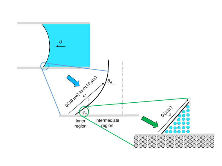
Figure 1: Length scales involved in flows with moving contact line

Hydrodynamic theories have been developed to understand the MCL problem via matched asymptotic techniques. Figure 1 illustrates the length scales that are involved in the MCL problem. In the method of matched asymptotic expansions, the solution within the inner region near the contact line is matched to the outer region through an intermediate region which is the region that is geometry-independent and where viscous and capillary forces are of comparable magnitude. With the assumption of low capillary numbers (${Ca\leq 0.1}$) and smooth flat solid surface, Cox [9] developed a theory that relates the contact angle at the intermediate region to the inner-scale contact angle:

$$g(\theta_{d},\mu_{2}/\mu_{1})=g(\theta_{w},\mu_{2}/\mu_{1})+\text{Ca}_{d}\ln\bigg{(}\frac{d}{\lambda}\bigg{)}+\text{Ca}_{d}Q_{int},$$ (9)

where the function ${g}$ is expressed as:

$$g(\theta,\mu_{2}/\mu_{1})=\int_{0}^{\beta}\bigg{(}\frac{d\beta}{f(\beta,\mu_{2}/\mu_{1})}\bigg{)},$$ (10)

and

$$f(\beta,\mu_{2}/\mu_{1})=\frac{2\sin\beta\bigg{[}\big{(}\mu_{2}/\mu_{1}\big{)}^{2}\big{(}\beta^{2}-\sin^{2}\beta\big{)}+2\big{(}\mu_{2}/\mu_{1}\big{)}\big{[}\beta(\pi-\beta)+\sin^{2}\beta\big{]}+\big{[}(\pi-\beta)^{2}-\sin^{2}\beta\big{]}\bigg{]}}{\big{(}\mu_{2}/\mu_{1}\big{)}\big{(}\beta^{2}-\sin^{2}\beta\big{)}\big{[}(\pi-\beta)+\sin\beta\cos\beta\big{]}+\big{[}(\pi-\beta)^{2}-\sin^{2}\beta\big{]}(\beta-\sin\beta\cos\beta\big{)}}.$$

In equation 9, ${\mu_{1}}$ is the viscosity of the displacing fluid, ${\mu_{2}}$ is the viscosity of the displaced fluid, ${\theta_{d}}$ is the contact angle at the intermediate scale, ${\theta_{w}}$ is the contact angle within the inner region, ${\text{Ca}_{d}}$ is the capillary number corresponding to the intermediate scale, ${d}$ is the radial distance from the contact line triple point to the intermediate contact angle ${\theta_{d}}$, ${\lambda}$ is the cut-off length scale determining the limit of continuum hydrodynamics, and ${Q_{int}}$ is a higher-order approximation term on the order of $O(Ca)$ [9]. ${\lambda}$ is a physical parameter corresponding to a molecular process, which both Cox [9] and Voinov [49] assumed to be the slip length, and it is at the order of few times the size of a fluid molecule. ${\theta_{w}}$ is still difficult to experimentally measure, but is usually assumed to be ${\theta_{eq}}$ for viscous flows [5]. The assumption of $\theta_{w}=\theta_{eq}$ has been supported by various experiments [20, 44]. ${Q_{int}}$ is an asymptotic ${O(Ca)}$ term that depends on the slip-length ${\lambda}$, viscosities ${\mu_{2}/\mu_{1}}$, and ${\theta_{w}}$, which is important for matching asymptotic theory with numerical results as shown in [46]. Hocking and Rivers [19] computed the second order leading term (${Q_{i}}$ which is ${Q_{int}-1}$) based on ${\theta_{w}}$ and the assumption of slip mechanism and negligible ${\mu_{2}}$. When the viscosity of the displacing fluid is much larger than that of the displaced fluid, i.e. negligible ${\mu_{2}/\mu_{1}}$, equation 10 simplifies to:

$$g(\theta)=\frac{1}{2}\int_{0}^{\beta}\bigg{(}\frac{\beta-\sin\beta\cos\beta}{\sin\beta}\bigg{)}d\beta.$$ (11)

Moreover, when ${\theta_{d}\leq 3\pi/4}$ equation 9 becomes [49]:

$$\theta_{d}^{3}=\theta_{eq}^{3}+Ca_{d}\bigg{[}9\bigg{(}\ln\frac{d}{\lambda}\bigg{)}+Q_{int}\bigg{]}.$$ (12)

The above equation describes the relation between the intermediate contact angle, ${\theta_{d}}$, and ${\theta_{eq}}$ for ${Ca_{d}\leq 0.1}$, smooth surface, small ${\mu_{2}/\mu_{1}}$, and ${\theta_{d}\leq 3\pi/4}$.

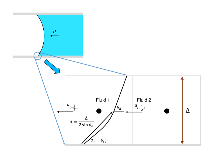
Figure 2: The implementation of dynamic contact angle in grid points near the contact line

The numerical implementation of equation 12 is illustrated in Figure 2. The local capillary number, $Ca_{d}=\mu U_{d}/\gamma,$ is computed by averaging the parallel wall velocities in the cell containing the contact line, that is $U_{d}=(u_{i-1/2,1}+u_{i+1/2,1})/2$. We have observed that using this form of the averaged velocity to determine the local capillary number produces less spurious currents compared with a linear interpolation of velocity at the interface. The radial distance, $d$, is calculated as shown in Figure 2 which depends on the grid size and corresponds to the intermediate length scale. After $\theta_{d}$ is determined, the normal vector in the cells neighboring the contact line is computed via:

$$\vec{n} = \vec{n}_{||}\sin\theta_{d}+\vec{n}_{\perp}\cos\theta_{d},$$ (13)

where $\vec{n}_{||}$ and $\vec{n}_{\perp}$ are parallel and normal solid surface vectors. Once the normal vector is determined, the curvature is computed

$$\kappa=\nabla\cdot\vec{n}=\frac{\partial n_{x}}{\partial x}+\frac{\partial n_{y}}{\partial y}.$$ (14)

Equation 14 is discretized using central differences as mentioned in section 2. However, for grid cells near the wall, the derivative of the normal in the direction perpendicular to the wall is discretized using a one-sided stencil. The one-sided finite-difference provided more accurate results in terms of both spurious currents and curvature when it was compared with central finite difference which requires defining ghost cell points below the wall. The next section illustrates the reinitialization of level-set field and how contact angle boundary condition is taken into consideration.

3.2 Level-set reinitialization with contact angles

Computing the signed distance function based on point-wise, piecewise linear, and smooth reconstruction of the interface from the level-set function is elaborated in details in [35]. In our numerical method, piecewise linear interface reconstruction (called P₂ in [35]) is used to compute signed distance function. First, the discrete interface points corresponding to ${f(\mathbf{x})=0}$ is found from level-set. The discrete interface points are determined when values of the level-set defined on grid points change sign in x and y directions. Then, three discrete points that have the shortest distances to the grid point are determined (see Figure 3):

$$|\mathbf{x}_{i,j}-\mathbf{x}_{1}|<|\mathbf{x}_{i,j}-\mathbf{x}_{2}|<|\mathbf{x}_{i,j}-\mathbf{x}_{3}|.$$ (15)

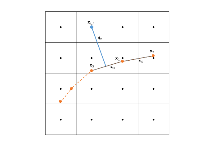
Figure 3: Piecewise linear projection to compute the distance from a grid point to a reconstructed piecewise linear function

Afterward, the minimal distance ${\mathbf{d}_{2}=d_{i,j}}$ to the piecewise linear reconstructed interface from the three points ${\mathbf{x}_{1},\mathbf{x}_{2}}$, and ${\mathbf{x}_{3}}$ is computed through normal projection of $\mathbf{x}_{i,j}$. The minimal distance ${\mathbf{d}_{2}}$ normally intersects one of the segments ${s_{13}}$ or ${s_{12}}$. The normal distance from a point ${x_{i,j}}$ with coordinates ${(x_{i},y_{i})}$ to a line containing two points ${\mathbf{x}_{1}}$ and ${\mathbf{x}_{3}}$, with coordinates ${(x_{1},y_{1})}$ and ${(x_{3},y_{3})}$ respectively, is:

$$\mathbf{d}_{2}=\frac{|(x_{i}-x_{3})(y_{1}-y_{i})-(x_{i}-x_{1})(y_{3}-y_{1})|}{\sqrt{(y_{3}-y_{1})^{2}+(x_{3}-x_{1})^{2}}}.$$ (16)

The above distance formula is applied for each segment ${s_{12}}$ and ${s_{13}}$. In Figure 3, ${\mathbf{d}_{2}}$ normally intersects ${s_{13}}$ such that ${\mathbf{d}_{2}\cdot\mathbf{t}_{13}=0}$, where ${t_{13}}$ is the tangent vector to the segment ${s_{13}}$.

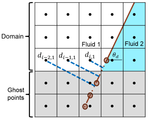
Figure 4: Piecewise linear projection to compute the distance from a grid point to a reconstructed piecewise linear function with contact angle boundary condition

When the interface intersects the solid surface, a contact angle boundary condition needs to be imposed. Figure 4 shows a schematic of how the distance function is constructed and computed when the interface intersects the solid boundary at a specified contact angle. The interface is extended linearly with a slope determined by the contact angle, so that reinitialization and distance computation is done correctly for grid points located near the contact line as illustrated in [43]. The contact angle with the level-set method was implemented in the framework of PDE-based reinitialization [43, 38]. In our approach, the extension of the interface is accomplished by linearly constructing the interface from the intersection points in the ghost domain. For instance, the values of $d_{i-2,1}$, $d_{i-1,1}$, and $d_{i,1}$ represent the respective distances from the linear extension of the contact line beyond the wall. In the algorithm, the level-set function is not defined in the ghost points as there is no need to do so because the curvature is computed by one-sided differences as explained in section 3.1. The location of the intersection points along the x-direction (brown circles in Figure 4) are determined via:

$$x_{lin,n}=x_{cl}-\left(\frac{\Delta}{\tan\theta}\right)k,$$ (17)

and

$$y_{lin,n}=y_{i}-\left(\Delta\right)k,$$ (18)

where ${x_{cl}}$ is the contact line defined at the grid-scale, and ${k}$ is an index between 1 and the number of intersection points in the x-direction. In the y-direction, the location of the intersection points (blue circle in Figure 4) are:

$$x_{lin,n}=x_{i+1-k},$$ (19)

and

$$y_{lin,n}=(x_{cl}-x_{i+1-k})\tan{\theta},.$$ (20)

Because curvature calculation involves a 5-point stencil, the minimum number of intersection points in each direction is three (which is the number that has been used in section 4) to have correct reinitialization for cells near the contact line. Once the interface is extended along the contact angle and the intersection points are determined, the distance values at grid points inside the domain are computed via piecewise linear interface reconstruction as in equation 16.

4 Results

This section describes the results obtained using the new approach presented above. We start by first considering the performance of the method for problems that do not involve contact angles, for which the accuracy of piecewise linear interface projection is investigated with the help of static and oscillating droplet problems.

4.1 Static droplet

In the static droplet problem, we test whether our new method allows the spurious currents to be on the order of machine precision, indicating an exact balance between the surface tension force and the pressure jump. It is well known [1] that such an exact balance cannot be achieved when the Hamilton-Jacobi reinitialization (PDE-based) procedure is used together with the ghost-fluid method. The balance between the pressure jump across the droplet and the surface tension force has been achieved only when reinitialization step is not applied [1]. When PDE-based reinitialization is used, the interface is slightly perturbed, and the reinitialization process has to be modified at grid points by manually propagating characteristics based on the interface location [41]. On the other hand, the method of reinitialization used in this work allows the surface tension and the pressure jump to be balanced to machine precision. Figure 5 shows that with our approach, the maximum velocity converges to machine precision for different grid sizes. The results have been obtained by solving for the velocity field as well as the pressure, and reinitialization is carried out at every time-step. The dimensionless Laplace number, defined as the ratio of the Reynolds and capillary numbers, is suitable for characterizing the flow behavior:

$$La=\frac{\rho L\gamma}{\mu^{2}}=\frac{Re}{Ca},$$ (21)

where ${L}$ is the characteristic length-scale, which is equal to the interface radius. In this test, La = 12000, which is the same number as the static droplet test case conducted in [34]. The capillary waves triggered by initial local numerical curvature errors can be observed as periodic oscillations. Also, the initial numerical error decreases with grid refinement. This example shows how the level-set method with piecewise linear interface reconstruction balances the pressure jump and the surface tension for the static droplet case.

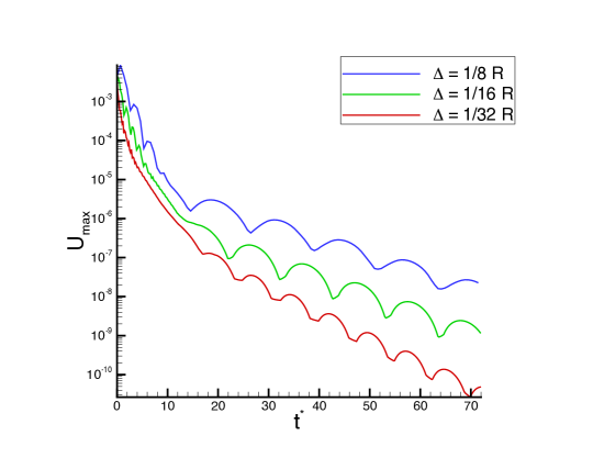
Figure 5: Velocity convergence to zero for static droplet at different grid sizes

4.2 Oscillating droplet

When the droplet is slightly perturbed, the physical imbalance between the pressure jump and the surface tension gives rise to a restoring flow field that tends to drive the droplet back towards its equilibrium configuration. Lamb [29] derived an analytical solution for the frequency and the amplitude of a perturbed viscous droplet in vacuum. For a 2D droplet, the oscillation frequency of the second mode $\omega_{2}$, is $\sqrt{\frac{6\gamma}{\rho R^{3}}}$ and the decay rate for both amplitude and kinetic energy is proportional to $\exp\left(-\frac{4\mu}{\rho R^{2}}t\right)$. Figures 6 and 7 show the droplet amplitude and kinetic energy when the amplitude is perturbed by a factor of 1.04 relative to the equilibrium droplet. The domain size is ${4R}\times$$4R$, and the problem is characterized by Reynolds number $Re=\frac{\rho UL}{\mu}$ for the decay rate and Weber number $We=\frac{\rho U^{2}L}{\gamma}$ for the oscillation frequency. Table 1 lists the fluid parameters which correspond to $We=1$ and $Re=200$. The Laplace number for this case is $La=40000$. The viscosity and density ratio between the droplet and its surrounding is 1/1000. Both the amplitude and the kinetic energy approach the upper limit of the decay rate, and the time period of oscillation matches the analytical solution. The solution becomes more accurate as the grid is refined, and that shows that the numerical method converges to the analytical solution.

R (mm)	$\rho$ (kg/m3)	$\mu$ (cP)	$\gamma$(mN/m)
1	1000	1	40

Table 1: Fluid properties corresponding to Re = 200 and We = 1

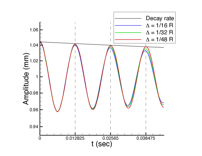
Figure 6: Grid convergence of droplet amplitude to analytical solution for Re = 200 and We = 1

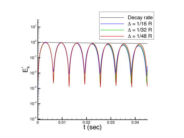
Figure 7: Grid convergence of droplet energy to analytical solution for Re = 200 and We =1

4.3 Moving Wedge

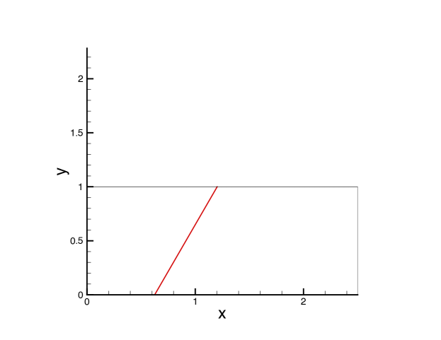
Figure 8: Moving wedge: linear interface tilted at angle ${\theta=60}$

To test the piecewise linear projection method with the contact line implementation, the translating wedge is tilted at an angle in uniform flow from left to right as shown in Figure 8. The wedge should maintain its orientation with respect to the initially imposed angle, such that the flow field is not disturbed. The numerical method, including the coupling of Navier-Stokes, level-set advection, and piecewise linear reconstruction is employed. The inflow capillary and Reynolds number are ${Ca=0.01}$ and ${Re=1}$ respectively. Table 2 shows velocity and curvature errors in ${L_{2}}$ and ${L_{\infty}}$ norms at dimensionless time ${t^{*}=1}$, time normalized by ${L/U}$, for different grid sizes where $L$ is the domain width. The grid size ${\Delta}$ is the unit length of the domain divided by the number of grid cells. The velocity and curvature error norms have been computed as follows:

$$||\mathbf{u}-\mathbf{\tilde{u}}||_{2}=\sqrt{\frac{1}{n}\sum_{i,j}(\mathbf{u}_{i,j}-\mathbf{\mathbf{\tilde{u}}}_{i,j})^{2}},$$ (22)

$$||\mathbf{u}-\mathbf{\tilde{u}}||_{\infty}=\max_{i,j}(|\mathbf{u}_{i,j}-\mathbf{\mathbf{\tilde{u}}}_{i,j}|),$$ (23)

$$||\kappa_{\Gamma}-\widetilde{\kappa}_{\Gamma}||_{2}=\sqrt{\frac{1}{n_{\Gamma}}\sum_{n_{\Gamma}}(\kappa_{\Gamma_{k}}-\widetilde{\kappa}_{\Gamma_{k}})^{2}},$$ (24)

$$||\kappa_{\Gamma}-\widetilde{\kappa}_{\Gamma}||_{\infty}=\max_{\Gamma}(|\kappa_{\Gamma_{k}}-\widetilde{\kappa}_{\Gamma_{k}}|),$$ (25)

	${||\mathbf{u}-\mathbf{\tilde{u}}||}$		${||\mathbf{\kappa_{\textrm{$\Gamma$}}}-\widetilde{\kappa}_{\Gamma}||}$
${\Delta}$	${L_{2}}$	${L_{\infty}}$	${L_{2}}$	${L_{\infty}}$
1/20	4.60E-9	1.50E-8	7.23E-8	1.27E-7
1/40	4.20E-9	1.11E-8	5.42E-8	1.26E-7
1/60	3.45E-9	8.76E-9	5.39E-8	9.32E-8
1/80	3.34E-9	8.75E-9	4.59E-8	8.53E-8

Table 2: ${L_{2}}$ and ${L_{\infty}}$ error of velocity and curvature in moving wedge for angle ${\theta=60}$ at ${t^{*}=1}$

where the curvature is computed at the interface, which is interpolated from level-set values. It can be seen that the error is very small and decreases with grid refinement.

4.4 Static Parabolic Interface

The second verification test is the static fluid parabolic interface intersecting the domain border at an imposed angle (see Figure 11 for interface shape). There is no-flow at the left and right boundaries, and free-slip is imposed at the bottom and top boundaries. Again, the pressure and velocity fields are computed and the accuracy of the method is characterized by the velocity and curvature error norms. The Laplace number is chosen to characterize the flow behavior, where ${L}$ is a characteristic length scale equal to the interface radius when ${\theta=60}$. In this test, La = 12000 which is similar to the static droplet test case in section 4.1. Figure 9 shows the evolution of maximum velocity (scaled by ${U}$) with respect to the dimensionless time $t^{*}$ for a circular interface at ${\theta=60}$. The capillary waves converge with grid refinement, which is similar to the case for the static droplet as illustrated above in Figure 5. In addition, The maximum velocity converges to machine precision as shown in Figure 10. Tables 3 and 4 show the velocity, as well as the curvature error norms for different imposed contact angles. The velocity converges when the grid is refined for the considered contact angles. However, the velocity error increases as the contact angle decreases because the interface is more curved when the angle approaches zero and the linear extension of the interface near the border becomes less accurate [43]. Table 4 indicates that the curvature does not converge with grid refinement because the linear extension of the interface used for piecewise projection introduces a jump in curvature at the interface. However, the error magnitude remains relatively small.

	$\theta=60$		$\theta=45$		$\theta=30$
$\Delta$	$L_{2}$	$L_{\infty}$	$L_{2}$	$L_{\infty}$	$L_{2}$	$L_{\infty}$
1/20	4.08E-4	1.28E-3	7.15E-4	2.16E-3	2.89E-3	1.50E-2
1/40	1.14E-4	3.51E-4	3.47E-4	1.20E-3	9.29E-4	3.95E-3
1/60	6.04E-5	2.14E-4	1.99E-4	8.35E-4	6.03E-4	2.29E-3
1/80	2.41E-5	7.35E-5	1.28E-4	4.45E-4	5.36E-4	2.23E-3

Table 3: Velocity ${L_{2}}$ and ${L_{\infty}}$ error in static parabolic interface for different angles at ${t^{*}=1}$

	$\theta=60$		$\theta=45$		$\theta=30$
$\Delta$	$L_{2}$	$L_{\infty}$	$L_{2}$	$L_{\infty}$	$L_{2}$	$L_{\infty}$
1/20	3.09E-3	3.62E-3	5.11E-3	3.70E-3	5.66E-3	1.55E-2
1/40	9.84E-4	1.41E-3	1.93E-3	2.33E-3	4.37E-3	6.74E-3
1/60	8.02E-4	8.67E-4	1.22E-3	1.66E-3	5.56E-3	6.64E-3
1/80	4.78E-4	6.45E-4	1.80E-4	2.96E-4	4.98E-3	5.25E-3

Table 4: Curvature ${L_{2}}$ and ${L_{\infty}}$ error in static parabolic interface for different angles at ${t^{*}=1}$

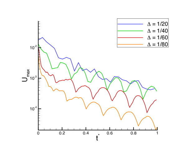
Figure 9: Convergence of spurious currents for the static parabolic interface intersecting the domain boundary at angle ${\theta=60}$

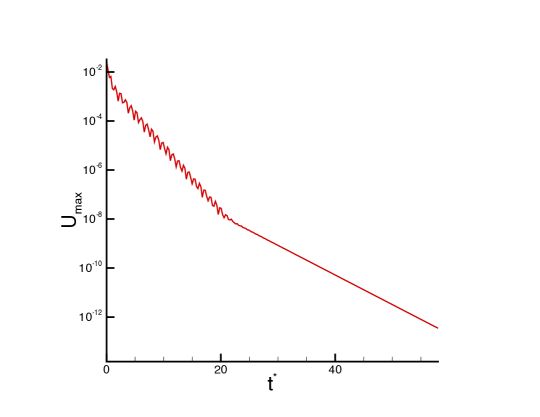
Figure 10: Convergence of spurious currents to machine precision for the static parabolic interface intersecting the domain boundary at angle ${\theta=60}$ (${\Delta=1/60}$)

4.5 Moving Parabolic Interface

In this test, a parabolic interface is advected in a uniform constant flow. There have been several attempts to analyze the accuracy of the algorithm in terms of spurious currents for the translating droplet [34, 1, 36]. However, to the best of our knowledge, the translating parabolic interface with an imposed contact angle coupled with Navier-Stokes has not been tested. The static parabolic interface has been analyzed with the conventional PDE-based reinitialization modified to consider contact angle [38], but the magnitude of spurious currents was not reported. Figure 11 shows that the flow streamlines are slightly bent around the interface due to the presence of spurious currents. Table 5 shows the velocity and curvature errors at ${t^{*}=1}$ with $La$ = 12000 and $We$ = 0.4. The numerical method converges upon grid refinement for velocity as shown in Table 5; however, the curvature error does not converge with grid refinement. This is also due to the fact that the interface is linearly extended below the computational domain. The maximum curvature error has been computed without piecewise interface reconstruction, which is shown in the last column of table 5, and it converges with grid refinement.

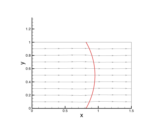
Figure 11: Streamlines for the moving parabolic interface intersecting the domain boundary at angle ${\theta=60}$

	${||\mathbf{u}-\mathbf{\tilde{u}}||}$		${||\mathbf{\kappa_{\textrm{$\Gamma$}}}-\widetilde{\kappa}_{\Gamma}||}$
${\Delta}$	${L_{2}}$	${L_{\infty}}$	${L_{2}}$	${L_{\infty}}$	${L_{\infty}}$ without proposed reinitialization
1/20	2.05E-3	1.14E-2	8.97E-3	1.80E-2	N/A
1/40	9.62E-4	5.13E-3	5.93E-3	1.44E-2	1.08E-2
1/60	7.14E-4	2.83E-3	4.56E-3	1.66E-2	4.41E-3
1/80	6.11E-4	2.33E-3	5.11E-3	1.68E-2	2.46E-3

Table 5: ${L_{2}}$ and ${L_{\infty}}$ error of velocity and curvature in moving parabolic interface for angle ${\theta=60}$ at ${t^{*}=1}$

4.6 Advancing interface in a capillary tube

In this validation example, the displacement of a wetting fluid by a non-wetting fluid in a capillary tube is investigated and compared with experiments from [20]. Also, the result is compared with the solution of ordinary differential equation boundary-value-problem derived for low capillary number steady-state interface in a capillary tube [37]. Table 6 lists parameters for the two cases considered in [20]. Both correspond to different equilibrium contact angles. The radius of the capillary tube is ${r=1}$ mm. Only half of the capillary tube is simulated, and symmetry boundary condition is applied at the center of the tube. The inlet boundary condition is a parabolic velocity (Poiseuille flow). The computational domain size is ${1.5r}\times$ ${r}$, which is found to be sufficient for a steady-state solution. The Cox-Voinov dynamic contact angle model is implemented with Navier slip-length of $\lambda={10^{-9}}$ m. The results are analyzed by considering the convergence of the interface shape to the theoretical solution of equation (1) in [37], which is:

$$\frac{{1}}{1-x}\frac{d[(1-x)\cos(\theta)]}{d(1-x)}=Ca\frac{{2\sin^{2}(\theta)}}{\theta-\sin(\theta)\cos(\theta)}\frac{1}{x}+B,$$ (26)

where $\theta=\frac{\pi}{2}$ at $x=1$, and $\theta=\theta_{w}$ at $x=\lambda$. The parameter $B$ is a constant that is part of the solution, and $x$ is the vertical distance from the wall to the tube-center. The macroscopic contact angle, which is computed at a vertical distance of 0.05 mm from the interface to the wall, is compared as well. Figure 12 shows that the interface converges to a steady state shape as the grid is refined for case 1. Figure 13 illustrates the effect of the high order asymptotic term in Cox-Voinov asymptotic theory. It can been seen that the high order term is required for case 1 to match the theoretical solution. As for case 2, the high order term corresponding to ${\theta_{w}=69}$ in Table 1 of Hocking [19] is small (${Q_{int}=0.35}$) compared to the first case (${Q_{int}=-2.4}$). Figure 14 shows a comparison between the numerical solution (with and without the higher order correction term) with the theoretical solution. The difference between the shapes is almost negligible.

The computed macroscopic contact angle is compared with the observed experimental results in [20]. The last two columns in Table 6 include the computed macroscopic angle and the observed experimental macroscopic contact angle. The difference between the computed and experimental macroscopic is around the 5% error measurement mentioned in [20].

	Ca	$\theta_{eq}$	$\theta_{macro}$ sim.	$\theta_{macro}$ exp.
Case 1	1.83E-2	0	67.6	66.5
Case 2	4.94E-2	69	107.1	114

Table 6: Simulation and experimental macroscopic contact angle for two different cases in [20]

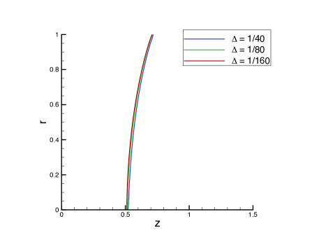
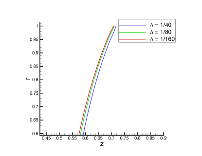
(a) The upper part of the steady-state interface	(b) Zoomed in near the contact angle

Figure 12: Interface steady-state shape convergence for different grid sizes for case 1

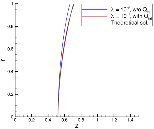
Figure 13: The effect of the high order term ${Q_{int}}$ and comparison with the theoretical solution for case 1

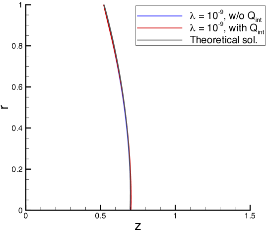
Figure 14: The effect of the high order term ${Q_{int}}$ and comparison with the theoretical solution for case 2

4.7 Capillary rise

In this example, our new method is used to model meniscus rise in a vertical tube. When a vertical capillary tube is brought in contact with a wetting fluid, the fluid spontaneously rises through the tube. The final location of the fluid interface is reached whenever the capillary pressure is balanced by gravity:

$$P_{c}=\frac{2\gamma\cos\theta_{eq}}{R}=\rho gh,$$ (27)

where ${h}$ is the final height of the fluid interface. The dynamics of the fluid interface between the initial fluid tube contact and the capillary-gravity balance can only be predicted accurately by modeling the correct physics of contact line dynamics. The simulation results are compared with recent experiment in [17], and Table 7 shows the fluid parameters for the relevant case. Symmetry boundary condition is imposed at the center of the tube, and atmospheric pressure boundary conditions are applied at the inlet and outlet of the domain. The Cox-Voinov model with slip-length ${\lambda=10^{-9}}$ m is used for the moving contact line. Figure 15 illustrates the interface shape when it is rising at two different times as well as when it reaches the final equilibrium state. The time evolution of the average fluid interface is compared with data taken from Figure 5 in [17]. In addition, the interface height is also tracked when a constant contact angle boundary condition is applied instead of the Cox-Voinov model. From Figure 16, it is seen that the numerical method with Cox-Voinov model predicts the trend of experimental measurements with slight difference. The discrepancy occurs at the beginning, and most likely this is when inertia plays a role in the dynamics where the Cox-Voinov model does not take into account. On the other hand, applying a constant contact angle without resolving the slip length results in an interface overshoot above the equilibrium height, which is inaccurate and unphysical.

$\theta_{eq}$	R (mm)	$\rho$ (kg/m3)	$\mu$ (cP)	$\gamma$(mN/m)
0	0.65	744	2.6	24.8

Table 7: Fluid properties corresponding to Soltrol 170 [17]

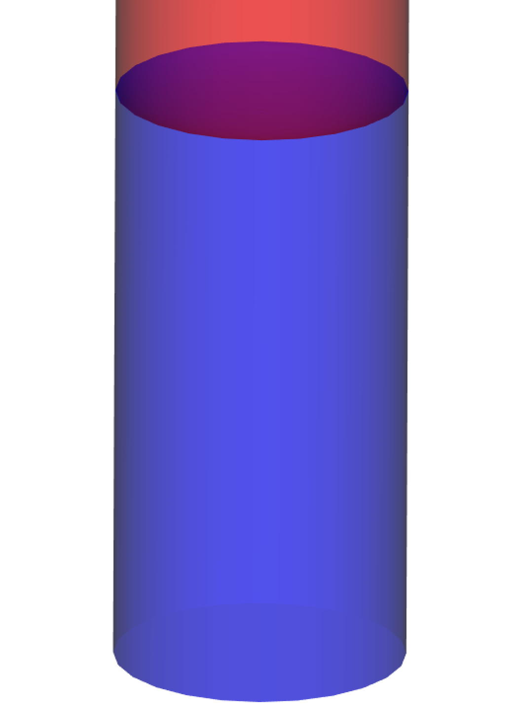
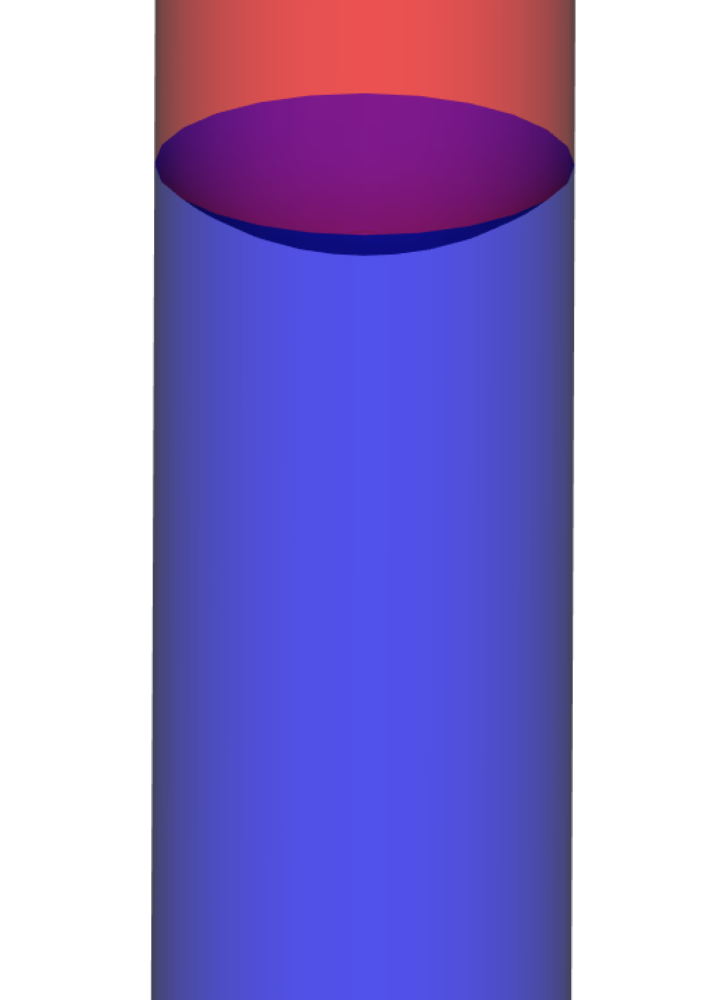
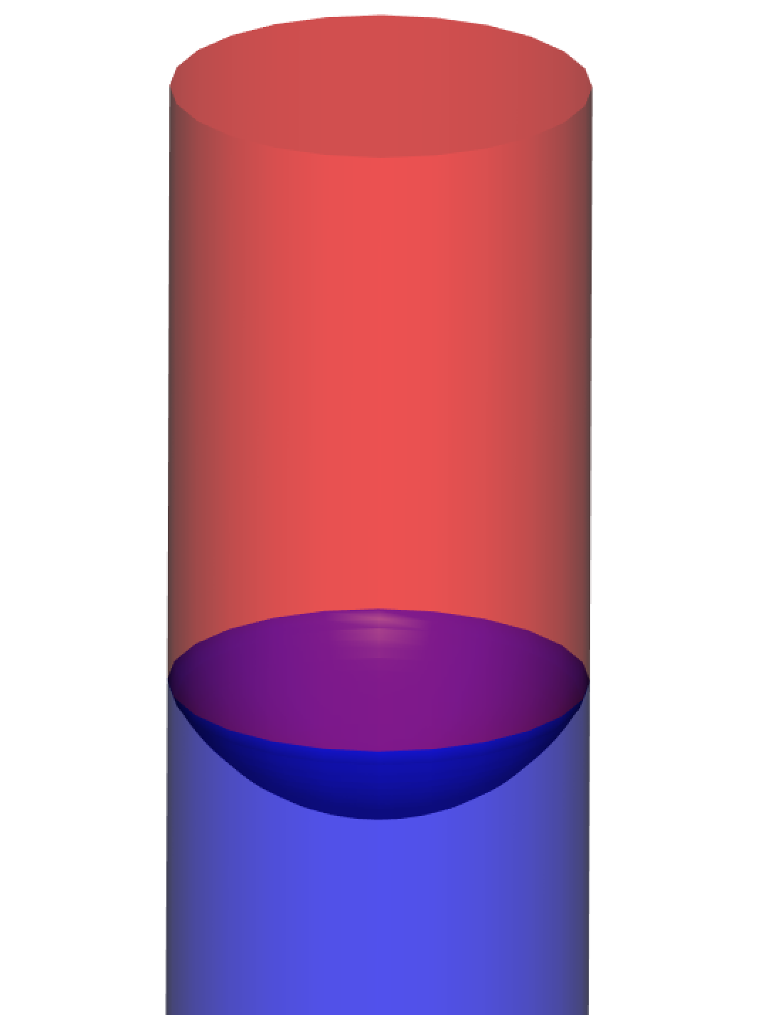
(a) The most deformed	(b) The deformed interface	(c) The final equilibrium interface
interface at t = 0.01 second	at t = 0.05 seconds	shape at t = 0.4 seconds

Figure 15: Interface shape at different stages (${\Delta=1/20}$)

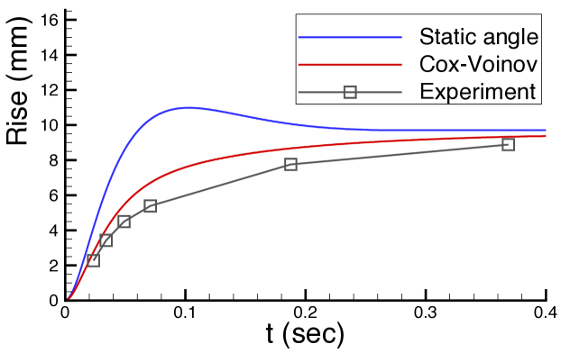
Figure 16: Average interface height vs. time for both static and dynamic angle (${\Delta=1/20}$) and comparison with experiment [17]

4.8 Forced imbibition of viscous oil by water

In this validation example, the forced displacement of a very viscous fluid inside a capillary tube is simulated. The results are compared with experiments by Hansen and Toong [14], where they showed schematics of the water/viscous oil interface shape at different capillary numbers. The wetting water displaces the non-wetting viscous oil, and large viscous bending occurs in the intermediate region. In addition, the displacement process is likely to become unstable because low viscous fluid (water) is injected into a higher viscous fluid (paraffin oil). Table 8 shows the parameters used to simulate this forced imbibition process. The contact angle has not been reported in [14]. They only mention that the capillary tube is more wetting towards the water. In the simulation, the contact angle is assumed to be $\theta_{eq}=70^{o}$ with respect to the water, which makes it the wetting fluid. Figure 17 shows the water/viscous-oil interface at two different capillary numbers. For case 1, the capillary number is Ca = 1.14E-3, where the viscosity of the injected fluid is used. The capillary number is sufficient enough to bend the fluid interface, and viscous fingering occurs as shown in Figure 17 (a). The results agree with the interface shape reported in the experiment at Ca = 1.14E-3 (Figure 6(d) in [14]). The computed macroscopic contact angle based on the Cox-Voinov theory is $\theta_{macro}=120^{o}$.

At Ca = 4.02E-4, the capillary force competes with the viscous force due to water injection. The viscous force bends the interface towards the oil side. However, the capillary force and the water wettability prefers to lower the system energy by minimizing the interfacial area. Therefore, the water/oil interface breaks into water droplets. The interface breakup is periodic as seen in Figure 17 (b). This complex interfacial dynamics of generating periodic droplets has also been reported in [14] at the same capillary number of Ca = 4.02E-4. The macroscopic contact angle in this case is $\theta_{macro}=115^{o}$. Figure 18 shows the convergence of the simulation results. It is also confirmed in this example that the Cox-Voinov model is necessary to match the experimental results. Applying a constant contact angle, without resolving the slip-length, results in a completely different fluid interface shape for both capillary numbers as shown in the black curves in Figure 18 .

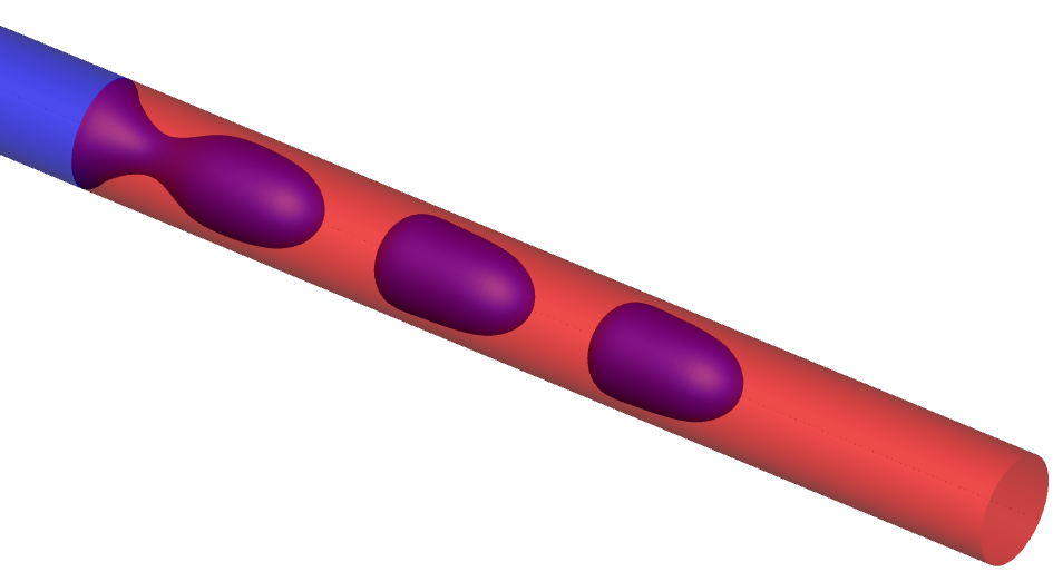
(a) Case 1: Ca = 1.14E-3	(b) Case 2: Ca = 4.02E-4

Figure 17: The water/oil interface shape that is deformed due to viscous forces at different capillary numbers

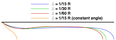
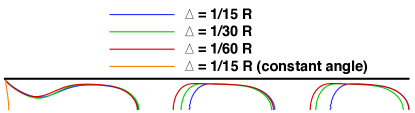
(a) Case 1: Ca = 1.14E-3	(b) Case 2: Ca = 4.02E-4

Figure 18: Interface shape convergence for different grid sizes

$\theta_{eq}$	R (mm)	$\rho_{w}/\rho_{o}$ (kg/m${}^{\text{3}}$)	$\mu_{w}/\mu_{o}$ (cP)	$\gamma$(mN/m)
70	1.23	993/874	0.99/177	51.9

Table 8: Fluid properties corresponding to water and paraffin oil (Nujol). The parameters are taken from [14]

.

5 Conclusion

A new numerical method based on linear reconstruction of the interface has been developed to simulate two-phase flow with moving contact lines. The method is accurate in terms of representing the fluid interface. In terms of spurious currents, the velocity error converges to machine precision for static interfaces that include contact angle boundary condition and the error decreases with grid refinement when the interface is advected in a constant velocity field. The method combined with the Cox-Voinov model is validated and compared with the theory for advancing interface in a capillary tube. The higher-order asymptotic term in method of matched asymptotic expansions in the Cox-Voinov model is necessary to match the theoretical solution for small contact angles. In addition, the method has been compared with experiments for both advancing fluid in a capillary tube and vertical capillary rise which shows good agreement.

References

- [1] Abadie, T., Aubin, J., and Legendre, D. On the combined effects of surface tension force calculation and interface advection on spurious currents within volume of fluid and level set frameworks. Journal of Computational Physics 297 (2015), 611 – 636.
- [2] Afkhami, S., Buongiorno, J., Guion, A., Popinet, S., Scardovelli, R., and Zaleski, S. Transition in a numerical model of contact line dynamics and forced dewetting. arXiv preprint arXiv:1703.07038 (2017).
- [3] Afkhami, S., and Bussmann, M. Height functions for applying contact angles to 2D VOF simulations. International Journal for Numerical Methods in Fluids 57, 4 (2008), 453 – 472.
- [4] Afkhami, S., Zaleski, S., and Bussmann, M. A mesh-dependent model for applying dynamic contact angles to VOF simulations. Journal of Computational Physics 228, 15 (2009), 5370 – 5389.
- [5] Bonn, D., Eggers, J., Indekeu, J., Meunier, J., and Rolley, E. Wetting and spreading. Rev. Mod. Phys. 81 (2009), 739 – 805.
- [6] Brackbill, J., Kothe, D., and Zemach, C. A continuum method for modeling surface tension. Journal of Computational Physics 100, 2 (1992), 335 – 354.
- [7] Chorin, A. J. A numerical method for solving incompressible viscous flow problems. Journal of Computational Physics 2, 1 (1967), 12 – 26.
- [8] Cinar, Y., and Riaz, A. Carbon dioxide sequestration in saline formations: Part 2: Review of multiphase flow modeling. Journal of Petroleum Science and Engineering 124 (2014), 381 – 398.
- [9] Cox, R. G. The dynamics of the spreading of liquids on a solid surface. part 1. viscous flow. Journal of Fluid Mechanics 168 (7 1986), 169–194.
- [10] de Gennes, P. G. Wetting: statics and dynamics. Rev. Mod. Phys. 57 (1985), 827 – 863.
- [11] Dupont, J. B., and Legendre, D. Numerical simulation of static and sliding drop with contact angle hysteresis. Journal of Computational Physics 229, 7 (2010), 2453 – 2478.
- [12] Dussan, E. B. On the Spreading of Liquids on Solid Surfaces: Static and Dynamic Contact Lines. Annual Review of Fluid Mechanics 11 (1979), 371 – 400.
- [13] Francois, M. M., Cummins, S. J., Dendy, E. D., Kothe, D. B., Sicilian, J. M., and Williams, M. W. A balanced-force algorithm for continuous and sharp interfacial surface tension models within a volume tracking framework. Journal of Computational Physics 213, 1 (2006), 141 – 173.
- [14] Hansen, R., and Toong, T. Interface behavior as one fluid completely displaces another from a small-diameter tube. Journal of Colloid and Interface Science 36, 3 (1971), 410–413.
- [15] Harlow, F. H., and Welch, J. E. Numerical calculation of time-dependent viscous incompressible flow of fluid with free surface. The physics of fluids 8, 12 (1965), 2182–2189.
- [16] He, W., Yi, J. S., and Van Nguyen, T. Two-phase flow model of the cathode of PEM fuel cells using interdigitated flow fields. AIChE Journal 46, 10 (2000), 2053 – 2064.
- [17] Heshmati, M., and Piri, M. Experimental investigation of dynamic contact angle and capillary rise in tubes with circular and noncircular cross sections. Langmuir 30, 47 (2014), 14151 – 14162.
- [18] Hirt, C. W., and Nichols, B. D. Volume of fluid VOF method for the dynamics of free boundaries. Journal of Computational Physics 39 (Jan. 1981), 201–225.
- [19] Hocking, L. M., and Rivers, A. D. The spreading of a drop by capillary action. Journal of Fluid Mechanics 121 (1982), 425 – 442.
- [20] Hoffman, R. L. A study of the advancing interface. I. interface shape in liquid-gas systems. Journal of Colloid and Interface Science 50, 2 (1975), 228 – 241.
- [21] Huh, C., and Scriven, L. Hydrodynamic model of steady movement of a solid/liquid/fluid contact line. Journal of Colloid and Interface Science 35, 1 (1971), 85 – 101.
- [22] Jacqmin, D. Calculation of two-phase Navier Stokes flows using phase-field modeling. Journal of Computational Physics 155, 1 (1999), 96 – 127.
- [23] Jiang, G.-S., and Shu, C.-W. Efficient implementation of weighted ENO schemes. Journal of Computational Physics 126, 1 (1996), 202 – 228.
- [24] Kang, M., Fedkiw, R. P., and Liu, X.-D. A boundary condition capturing method for multiphase incompressible flow. Journal of Scientific Computing 15, 3 (2000), 323–360.
- [25] Kistler, S., and Schweizer, P. Liquid Film Coating: Scientific Principles and Their Technological Implications. Chapman & Hall, 1997.
- [26] Kumar, S. Liquid Transfer in Printing Processes: Liquid Bridges with Moving Contact Lines. Annual Review of Fluid Mechanics 47 (2015), 67 – 94.
- [27] Lafaurie, B., Nardone, C., Scardovelli, R., Zaleski, S., and Zanetti, G. Modelling merging and fragmentation in multiphase flows with SURFER. Journal of Computational Physics 113, 1 (1994), 134 – 147.
- [28] Lake, L. Enhanced oil recovery. Prentice Hall, 1989.
- [29] Lamb, H. Hydrodynamics. University Press, 1916.
- [30] Legendre, D., and Maglio, M. Comparison between numerical models for the simulation of moving contact lines. Computers and Fluids 1, 0 (2014), –.
- [31] Liu, X.-D., Fedkiw, R. P., and Kang, M. A boundary condition capturing method for poisson’s equation on irregular domains. Journal of Computational Physics 160, 1 (2000), 151 – 178.
- [32] Moebius, F., and Or, D. Inertial forces affect fluid front displacement dynamics in a pore-throat network model. Phys. Rev. E 90 (2014), 023019.
- [33] Owkes, M., and Desjardins, O. A mesh-decoupled height function method for computing interface curvature. Journal of Computational Physics 281 (2015), 285 – 300.
- [34] Popinet, S. An accurate adaptive solver for surface-tension-driven interfacial flows. Journal of Computational Physics 228, 16 (2009), 5838 – 5866.
- [35] Qin, Z., Delaney, K., Riaz, A., and Balaras, E. Topology preserving advection of implicit interfaces on cartesian grids. Journal of Computational Physics 290 (2015), 219 – 238.
- [36] Raeini, A. Q., Blunt, M. J., and Bijeljic, B. Modelling two-phase flow in porous media at the pore scale using the volume-of-fluid method. Journal of Computational Physics 231, 17 (2012), 5653 – 5668.
- [37] Rame, E. On an approximate model for the shape of a liquid–air interface receding in a capillary tube. Journal of Fluid Mechanics 342 (1997), 87 – 96.
- [38] Rocca, G. D., and Blanquart, G. Level set reinitialization at a contact line. Journal of Computational Physics 265 (2014), 34 – 49.
- [39] Roman, S., Soulaine, C., AlSaud, M. A., Kovscek, A., and Tchelepi, H. Particle velocimetry analysis of immiscible two-phase flow in micromodels. Advances in Water Resources (2015).
- [40] Rowlinson, J., and Widom, B. Molecular Theory of Capillarity. Dover Publications, 2002.
- [41] Russo, G., and Smereka, P. A remark on computing distance functions. Journal of Computational Physics 163, 1 (2000), 51 – 67.
- [42] Snoeijer, J. H., and Andreotti, B. Moving Contact Lines: Scales, Regimes, and Dynamical Transitions. Annual Review of Fluid Mechanics 45 (2013), 269 – 292.
- [43] Spelt, P. D. A level-set approach for simulations of flows with multiple moving contact lines with hysteresis. Journal of Computational Physics 207, 2 (2005), 389–404.
- [44] Strom, G., Fredriksson, M., Stenius, P., and Radoev, B. Kinetics of steady-state wetting. Journal of Colloid and Interface Science 134, 1 (1990), 107 – 116.
- [45] Sui, Y., Ding, H., and Spelt, P. M. Numerical simulations of flows with moving contact lines. Annual Review of Fluid Mechanics 46, 1 (2014).
- [46] Sui, Y., and Spelt, P. D. An efficient computational model for macroscale simulations of moving contact lines. Journal of Computational Physics 242 (2013), 37 – 52.
- [47] Sussman, M., Smereka, P., and Osher, S. A level set approach for computing solutions to incompressible two-phase flow. Journal of Computational Physics 114, 1 (1994), 146 – 159.
- [48] Unverdi, S. O., and Tryggvason, G. A front-tracking method for viscous, incompressible, multi-fluid flows. Journal of computational physics 100, 1 (1992), 25 – 37.
- [49] Voinov, O. Hydrodynamics of wetting. Fluid Dynamics 11, 5 (1976), 714 – 721.
- [50] Wu, C., Young, D., and Wu, H. Simulations of multidimensional interfacial flows by an improved volume-of-fluid method. International Journal of Heat and Mass Transfer 60 (2013), 739 – 755.