Real frequency tearing layers with parallel dynamics and the effect on locking and resistive wall modes

Abstract

Tearing modes with real frequencies in the plasma frame (i.e. in addition to the Doppler shift due to $E\times B$ rotation) are of potential importance because of their effect on the locking process. In particular, it has recently been shown FinnColeBrennan that the Maxwell torque on the plasma in the presence of an applied error field is modified significantly for tearing modes having real frequencies near marginal stability. In addition, it is known FinnGerwinModeCoupling that resistive wall tearing modes can be destabilized below their no-wall limits by rotation, if the tearing modes have real frequencies near marginal stability. In this paper we first derive the tearing mode dispersion relation with pressure gradient, field line curvature and parallel dynamics in the resistive-inertial (RI) regime, neglecting the divergence of the $E\times B$ drift and perpendicular resistivity. The results show that the usual Glasser effect, a toroidal effect which involves real frequencies, occurs in this simplified model, which ignores perpendicular resistivity and the divergence of the $E\times B$ drift. We also find, using a similar simple model, the surprising result that in the viscoresistive regime with pressure gradient, favorable curvature due to toroidal effects, and parallel dynamics, a similar Glasser-like effect is found. We show that in both regimes the existence of tearing modes with complex frequencies is related to nearby electrostatic resistive interchange modes with complex frequencies. We discuss the effect on locking to an error field and the significant lowering of the threshold for destabilization of resistive wall tearing modes, which can be much more pronounced than the weak effect observed for RI tearing modes without pressure-curvature drive in Ref. FinnGerwinModeCoupling .

I Introduction

It is known that tearing modes can have real frequencies due to diamagnetism Coppi-1 ; Coppi-2 ; Biskamp ; FMA or pressure gradient and favorable curvature in the tearing layer, the Glasser effect GGJ1 ; GGJ2 . It has recently been discovered that the process of locking to an externally applied error field is affected strongly if the related spontaneous tearing modes have real frequencies FinnColeBrennan . Specifically, for a nearly marginally stable mode with real frequency $\omega_{r}$ in the plasma frame, $E\times B$ rotation leads to a peak in the reconnected flux near at the value of rotation $v$ such that the mode has zero frequency in the laboratory frame $\omega_{r}+kv=0$. That is, the flux is maximum when $v=-\omega_{r}/k$. Also, the Maxwell torque applied at the tearing layer is zero for $v=-\omega_{r}/k$ rather than zero at $v=0$. For this reason, the plasma should lock to the phase velocity of the tearing mode rather than to zero velocity FinnColeBrennan .

It is perhaps less appreciated that the qualitative behavior of tearing modes with real frequencies depends critically on parallel dynamics. For example, the Glasser effect, with pressure gradient and favorable field line curvature, is based on an intricate calculation involving full resistive MHD including parallel dynamics GGJ1 ; GGJ2 ; FinnManheimer . In this paper we show a streamlined derivation of the Glasser effect in the resistive-inertial (RI) tearing regime, in which ion inertia, but not ion viscosity, is included in resistive MHD. This simplified calculation based on reduced MHD includes parallel dynamics but neglects the divergence of the $E\times B$ drift $\nabla\cdot\mathbf{v}_{\perp}$ and the perpendicular resistivity $\eta_{\perp}$. The purpose of this derivation is threefold: (1) to show that these two last effects are not necessary to obtain the qualitative results, i.e. complex roots and stabilization for positive constant-$\psi$ matching parameter $\Delta^{\prime}$; (2) to illustrate this simple approach for use in other tearing regimes; and (3) to exploit the simplicity of this model to elucidate the physics. We use this simplified method to investigate the viscoresistive (VR) regime, which has perpendicular ion viscosity but neglects perpendicular ion inertia in the resistive MHD layer. These calculations include pressure gradient, favorable or unfavorable curvature and parallel dynamics.

In Sec. II we show our derivation of the RI regime in the presence of equilibrium pressure gradient and favorable or unfavorable field line curvature in the tearing layer. We show that the qualitative form for the tearing dispersion relation in this regime is obtained by adding only parallel dynamics and ignoring divergence of the $E\times B$ drift and the perpendicular resistivity (classical particle transport). The equations are derived by an extended reduced MHD formulation, in which specific effects are added one by one to the most primitive form of reduced MHD, making the terms representing the various physical effects evident. We have investigated the spontaneous tearing response, showing nonmonotonic behavior of the inner layer matching parameter $\Delta(Q)$ [c.f. Eq. (24)]. This behavior leads to the well-known complex roots, which occur in complex conjugate pairs. In addition to showing that $\nabla\cdot\tilde{\mathbf{v}}_{E}$ and $\eta_{\perp}$ are not required to obtain the qualitative behavior, the results of this section show how the relevant effects, e.g. pressure gradient and curvature and parallel dynamics, are added easily and transparently. In particular, we discuss the connection between the complex roots and nearby stable electrostatic resistive interchange modes with complex frequencies.

In Sec. III, we formulate the VR regime with pressure gradient, favorable curvature and parallel dynamics. We again neglect the divergence of the $E\times B$ drift and perpendicular resistivity, and use the methods outlined in Sec. II. The results show, surprisingly, that there is a large range of parameters for which $\Delta(Q)$ is again nonmonotonic, and this behavior again leads to complex conjugate roots and stabilization. We again explore the relationship between the electrostatic resistive interchange modes and (electromagnetic) tearing modes with complex frequencies.

In Sec. IV.1 we discuss error field penetration and locking for tearing layers whose spontaneous modes have non-zero real frequencies, e.g. the RI and VR models with Glasser effect. We also discuss, in Sec. IV.2, resistive wall tearing modes with such tearing layers. We show that for the ideal wall tearing mode near marginal stability with real frequency due to the Glasser effect, the resistive wall mode is destabilized below the no wall tearing threshold much more noticeably than in the RI regime without pressure-curvature drive FinnGerwinModeCoupling .

In Sec. V we summarize our results. On the basis of these results, we suggest that tearing modes typically have complex frequencies and their effects, namely finite velocity locking and destabilization of resistive wall modes for small $E\times B$ rotation. Lastly, we discuss other tearing regimes, of more possible relevance to high temperature plasmas, with complex frequencies.

II Resistive-inertial (RI) regime with pressure gradient and curvature

In this section we review the resistive-inertial (RI) tearing regime. We describe the equations in terms of “extended reduced resistive MHD”, i.e. we include effects beyond the most basic reduced resistive MHD model one at a time. In the first subsection we include the pressure-curvature term in the vorticity equation from the term proportional to $\mathbf{B}\times\boldsymbol{\kappa}\cdot\nabla p$, where $\boldsymbol{\boldsymbol{\kappa}}=\hat{\mathbf{b}}\cdot\nabla\hat{\mathbf{b}}$ is the field line curvature, using the advected pressure model ($\Gamma p_{0}\rightarrow 0$ in the adiabatic law.) The reduced resistive MHD model for tokamaks applies for large aspect ratio $R/r\gg 1$ so that, with $q(r)=rB_{z}/RB_{\theta}\gtrsim 1$, we can conclude that $B_{z}$ is large and constant, $B_{z}=B_{0}$. Toroidal geometry, specifically toroidal curvature of the field lines, is included to the degree that the average field line curvature in the layer, favorable where $q>1$, is included. We proceed to add parallel dynamics in the next subsection. The purpose of this section is to rederive known results with a simple and transparent model, so that it can be used to obtain new results in other regimes.

II.1 RI regime without parallel dynamics

The vorticity, parallel Ohm’s law, and the pressure equation, with $\tilde{\mathbf{B}}=\nabla\tilde{\psi}\times\hat{\mathbf{z}}$, $\tilde{\mathbf{v}}_{\perp}=\nabla\tilde{\phi}\times\hat{\mathbf{z}}$ in the RI regime (including ion inertia but with zero ion viscosity $\mu=0$) take the form

$$\rho\gamma\nabla_{\perp}^{2}\tilde{\phi}=iF\nabla_{\perp}^{2}\tilde{\psi}+\frac{2imB_{\theta}^{2}}{B_{0}^{2}r^{2}}\tilde{p},$$ (1)

$$\gamma\tilde{\psi}=iF\tilde{\phi}+\eta\nabla_{\perp}^{2}\tilde{\psi},\,\,\,\,\,\,\,\text{(a)}\,\qquad\gamma\tilde{p}=-\frac{imp^{\prime}}{r}\tilde{\phi},\,\,\,\,\,\,\,\text{(b)}$$ (2)

where $F(r)=\mathbf{k}\cdot\mathbf{B}=mB_{\theta}/r+kB_{0}$, $B_{z}=B_{0}$ is constant and the compression term proportional to $\Gamma p_{0}$ is not included. Close to the layer at $r=r_{t}$ we have $F(r)=\alpha x$ with $x=r-r_{t}$ and $\alpha=F^{\prime}(r_{t})=(B_{\theta}/r)(m-nq(r))^{\prime}=-(nB_{\theta}/r)q^{\prime}(r_{t})$. Again, we write $q=rB_{0}/RB_{\theta}$, and in cylindrical geometry the mode behaves as $\tilde{\mathbf{B}}=\tilde{\mathbf{B}}(r)e^{im\theta+ikz}$, with $k=-n/R$. In the close-in outer region, i.e. neglecting inertia and resistivity but still near the layer, we find

$$x(x\tilde{\phi})^{\prime\prime}-\frac{2m^{2}p^{\prime}(r_{t})}{B_{0}^{2}r_{t}n^{2}q^{\prime}(r_{t})^{2}}\tilde{\phi}=0,$$

or

$$(x^{2}\tilde{\phi}^{\prime})^{\prime}+D_{s}\tilde{\phi}=0,$$ (3)

where

$$D_{s}=-\frac{2m^{2}p^{\prime}(r_{t})}{B_{0}^{2}r_{t}n^{2}q^{\prime}(r_{t})^{2}}=-\frac{2r_{t}p^{\prime}(r_{t})}{B_{\theta}^{2}R^{2}q^{\prime}(r_{t})^{2}}$$ (4)

is the usual Suydam parameter and we have used $q(r_{t})=m/n$. In toroidal geometry this is replaced by the Mercier parameter GGJ1 ; GGJ2

$$D=\left(1-q(r_{t})^{2}\right)D_{s}.$$ (5)

For $p^{\prime}(r_{t})<0$ and $q(r_{t})>1$ we have favorable curvature, $D<0$. For normal profiles, we have $|D|\sim|D_{s}|\sim\beta\sim 2p/B_{0}^{2}\ll 1$. We will be more specific about the ordering of $\beta$ below. From Eq. (3) with $D_{s}\rightarrow D$ we have $\tilde{\phi}\propto x^{p}$ with $p=\left(-1\pm\sqrt{1-4D}\right)/2$. For $D\ll 1$ we have $p=-1,0$ and we can use the constant-$\psi$ approximation in the usual (zero pressure) way.

In the tearing layer we have

$$\rho\gamma\tilde{\phi}^{\prime\prime}=i\alpha x\tilde{\psi}^{\prime\prime}-E\tilde{\phi},\qquad\gamma\tilde{\psi}=i\alpha x\tilde{\phi}+\eta\tilde{\psi}^{\prime\prime},$$ (6)

where $E=-2m^{2}B_{\theta}^{2}(r_{t})p^{\prime}(r_{t})/\gamma B_{0}^{2}r_{t}^{3}=\alpha^{2}D_{s}/\gamma=E_{0}/\gamma$ and again toroidal geometry leads to $E_{0}\rightarrow\left(1-q(r_{t})^{2}\right)E_{0}$. Substituting, we find

$$\rho\gamma\tilde{\phi}^{\prime\prime}-\frac{\alpha^{2}x^{2}}{\eta}\tilde{\phi}+E\tilde{\phi}=\frac{i\alpha\gamma}{\eta}x\tilde{\psi}_{0},$$ (7)

where $\tilde{\psi}_{0}$ is the lowest order, constant part of $\tilde{\psi}$.

We let $x=\delta\xi$, defining $\delta$ by the first two terms, $\delta^{4}\alpha{}^{2}=\rho\gamma\eta$. With $\tilde{\phi}=-i\alpha\delta^{3}\tilde{\psi}_{0}W/\rho\eta=-i\gamma\tilde{\psi}_{0}W(\xi)/\alpha\delta$ we obtain

$$\frac{d^{2}W}{d\xi^{2}}-\xi^{2}W+GW=-\xi,$$ (8)

where

$$G=\frac{E\delta^{2}}{\rho\gamma},$$ (9)

and in toroidal geometry $G$ can contain the factor $1-q(r_{t})^{2}$. The scalings $E=E_{0}/\gamma$, $\delta\sim\gamma^{1/4}$ lead to $G\sim\gamma^{-3/2}$.

We do the usual constant-$\psi$ matching to find

$$\Delta^{\prime}=\Delta(\gamma)=\frac{[\tilde{\psi}^{\prime}]}{\tilde{\psi}_{0}}=\frac{1}{\eta\tilde{\psi}_{0}}\int\left(\gamma\tilde{\psi}_{0}-i\alpha x\tilde{\phi}\right)dx\,\,\,\,\,\text{or}$$

$$\Delta^{\prime}=\Delta(\gamma)=\frac{\delta\gamma}{\eta}\int_{-\infty}^{\infty}\left(1-\xi W\right)d\xi,$$ (10)

where $\Delta^{\prime}$ is obtained from the outer region. Then $\delta=\left(\rho\gamma\eta/\alpha^{2}\right)^{1/4}$ gives the RI constant-$\psi$ dispersion relation

$$\Delta^{\prime}=\left(\frac{\gamma^{5}\rho}{\alpha^{2}\eta^{3}}\right)^{1/4}\Delta_{s}=(\gamma\tau_{ri})^{5/4}\Delta_{s},\,\,\,\,\,\,\,\Delta_{s}\equiv\int_{-\infty}^{\infty}\left(1-\xi W\right)d\xi.$$ (11)

The constant-$\psi$ ordering parameter is $\Delta^{\prime}\delta=\epsilon$ and we have $\delta\sim\epsilon$, $\gamma\sim\epsilon^{3/2}$. Notice that in Eq. (8) the behavior $W\rightarrow 1/\xi$ as $\xi\rightarrow\infty$ is not affected by the presence of $G$, so that the integral for $\Delta_{s}$ still converges. For zero pressure we have the standard result $\Delta_{s}=2.12$. Otherwise, $W$ is influenced by $G$ and therefore $\Delta_{s}$ is changed. We have defined $\gamma_{ri}=1/\tau_{ri}$ by $\gamma_{ri}^{5}\rho/\alpha^{2}\eta^{3}=1$ or $\gamma_{ri}=\left(\eta^{3}\alpha^{2}/\rho\right)^{1/5}$ and $\gamma=\gamma_{ri}Q$ or $\gamma\tau_{ri}=Q$, with $Q\sim 1$. We have $\delta^{2}/\rho\gamma^{2}=\left(\eta/\alpha^{2}\rho(\gamma_{ri}Q)^{3}\right)^{1/2}$. With the above relations we obtain $\delta^{2}/\rho\gamma_{ri}^{2}=\left(1/\eta^{2}\rho\alpha^{8}\right)^{1/5}$ and

$$G=-\frac{2m^{2}B_{\theta}^{2}(r_{t})p^{\prime}(r_{t})}{B_{0}^{2}r_{t}^{3}}\frac{\delta^{2}}{\rho\gamma_{ri}^{2}}\frac{1}{Q^{3/2}}=\frac{G_{0}}{Q^{3/2}},$$ (12)

consistent with the scaling above. With these modifications, Eq. (11) becomes

$$\Delta^{\prime}=Q^{5/4}\Delta_{s}(Q)$$ (13)

and the effect of pressure is contained in $\Delta_{s}(Q)$. The ordering $\beta\sim\epsilon$, with $\delta\sim\epsilon\sim\eta^{2/5}$ and $\gamma\sim\epsilon^{3/2}$ shows $G_{0}=O(1)$. (This assumes $B_{\theta}/B_{0}\sim r_{t}/R$, which is small but of order unity with respect to $\epsilon$.)

As expected, the growth rate of the modes decreases for favorable curvature, $G_{0}<0$. That is, as $G_{0}<0$ decreases $\Delta_{s}(Q)$ increases, so the solution $Q$ to Eq. (13), decreases. (Not shown.) Similarly, for $G_{0}>0$, increasing $G_{0}$ causes an increase in $Q$.

In addition to the tearing modes which connect to the outer region ($\tilde{\psi}_{0}\neq 0$; electromagnetic tearing modes), there are localized electrostatic resistive interchange modes. These are solutions to the homogeneous form of Eq. (8). For $G_{0}>0$ (unfavorable curvature) these are Hermite functions $W(\xi)=H_{n}(\xi)e^{-\xi^{2}/2}$ with real eigenvalues

$$Q_{n}=\left(\frac{G_{0}}{2n+1}\right)^{2/3},$$ (14)

where we have used Eq. (12). These electrostatic interchanges have $\gamma_{es}=\gamma_{ri}Q_{n}$. This behavior $Q\sim|p^{\prime}|^{2/3}$ is well known, and these eigenvalues have an accumulation point at $Q=0$. Accordingly, the function $\Delta_{s}(Q)$ has poles on the positive real axis at these eigenvalues for $G_{0}>0$, with an accumulation point of poles $Q_{n}\rightarrow 0+$ at $Q=0$. The poles in $\Delta_{s}(Q)$ correspond only to eigenvalues with odd $n$, for which $W$ is odd in $\xi$. Similar behavior occurs in the work presented in Secs. II.2 and III.) For $G_{0}<0$, the poles are in the complex plane $Q\propto e^{\pm 2\pi i/3}$ with $\text{Re}(Q)<0$, corresponding to stable modes. Therefore, no clear evidence of these poles shows up in plots of $\Delta_{s}(Q)$ or $\Delta(Q)$ on the real $Q$ axis. We will return to the issue of these poles in Secs. II.2 and III.

II.2 RI regime with parallel dynamics

To include parallel dynamics, we take the model above, add parallel compression to the adiabatic law and include a parallel momentum equation,

$$\gamma\tilde{p}=-\frac{imp^{\prime}}{r}\tilde{\phi}-ik_{||}\Gamma p\tilde{v}_{||},$$ (15)

$$\rho\gamma\tilde{v}_{||}=-ik_{||}\tilde{p}-\frac{imp^{\prime}}{rB_{0}}\tilde{\psi}_{0},$$ (16)

where $k_{||}=F(r)/B_{0}$ and $\Gamma$ is the adiabatic index. Note that we have included parallel inertia but not parallel viscosity. In tearing modes driven by parallel velocity shear, the results using either sound wave dynamics (parallel inertia and pressure gradient) or parallel viscosity were found to be quite similar Finn-vparallel-prime . The $E\times B$ drift $\tilde{\mathbf{v}}_{\perp}=\nabla\tilde{\phi}\times\hat{\mathbf{z}}\rightarrow-\nabla\tilde{\Phi}\times\hat{\mathbf{z}}/B$, where $\tilde{\Phi}\approx-B\tilde{\phi}$ is the electrostatic potential, is incompressible in lowest order reduced MHD, where $B=|\mathbf{{B}|}$ equals $B_{0}$, which is constant. Extending reduced MHD to include $\nabla B\neq 0$ ($\nabla\cdot\tilde{\mathbf{v}}_{\perp}\approx-2\boldsymbol{\kappa}\cdot\nabla\tilde{\phi}\times\hat{\mathbf{z}}=-2\tilde{\mathbf{v}}_{\perp}\cdot\boldsymbol{\kappa}$) and the perpendicular resistivity $\eta_{\perp}$ (particle transport) gives all the terms in general compressible resistive MHD GGJ1 ; GGJ2 ; FinnManheimer . See Appendix A. We proceed without these effects and show that the known qualitative behavior is present without the effects of $\nabla\cdot\tilde{\mathbf{v}}_{\perp}$ and $\eta_{\perp}$. We find

$$\left(\begin{array}[]{cc}\rho\gamma&ik_{||}\\ ik_{||}\Gamma p&\gamma\end{array}\right)\left(\begin{array}[]{c}\tilde{v}_{||}\\ \tilde{p}\end{array}\right)=-\frac{imp^{\prime}}{r}\left(\begin{array}[]{c}\tilde{\psi}_{0}/B_{0}\\ \tilde{\phi}\end{array}\right)$$ (17)

and thus

$$\tilde{p}=-\frac{imp^{\prime}}{r}\frac{1}{\gamma^{2}+k_{||}^{2}c_{s}^{2}}\left(\gamma\tilde{\phi}-\frac{ik_{||}c_{s}^{2}}{B_{0}}\tilde{\psi}_{0}\right),$$ (18)

where $c_{s}^{2}=\Gamma p/\rho$ is the square of the sound speed. Referring to Eq. (2b), the first term here has $\tilde{\phi}/\gamma\rightarrow\gamma\tilde{\phi}/\left(\gamma^{2}+k_{||}^{2}c_{s}^{2}\right)$, and the sound wave propagator $\propto 1/\left(\gamma^{2}+k_{||}^{2}c_{s}^{2}\right)$ represents the stabilizing influence of the pressure perturbation leaking away along the field lines by sound wave propagation. The second term in Eq. (18) represents the tilting of the field lines by $\tilde{\psi}_{0}$ into the equilibrium pressure gradient. This effect gives an additional pressure perturbation of the same sign as the part proportional to $\tilde{\phi}$, e.g. destabilizing if $G_{0}>0$, but it is also mitigated by the sound wave propagator. These parallel dynamics terms are important unless $\gamma^{2}\gg k_{||}^{\prime 2}\delta^{2}c_{s}^{2}$, when the advected pressure model is regained. Also, even if $\gamma^{2}\ll k_{||}^{\prime 2}\delta^{2}c_{s}^{2}$, the advected pressure model holds in the ideal MHD outer region, where $\tilde{\psi}_{0}=ik_{||}B_{0}\tilde{\phi}/\gamma$.

Substituting (18) for (2b) and normalizing as before, we find that we must replace

$$GW\longrightarrow\frac{GQ^{2}}{Q^{2}+b^{2}\xi^{2}}W+\frac{Gb^{2}}{Q^{2}+b^{2}\xi^{2}}\xi$$ (19)

in Eq. (8), where

$$b^{2}=\alpha^{2}\delta^{2}c_{s}^{2}/\gamma_{ri}^{2}B_{0}^{2}=b_{0}^{2}Q^{1/2}$$ (20)

is dimensionless and $O(\beta)$. The last relation defining $b_{0}$ is valid because $\delta\sim\gamma^{1/4}$ in the RI regime. We find

$$\frac{d^{2}W}{d\xi^{2}}-\xi^{2}W+\frac{Q^{2}}{Q^{2}+b^{2}\xi^{2}}GW=-\left(1+\frac{Gb^{2}}{Q^{2}+b^{2}\xi^{2}}\right)\xi.$$ (21)

As discussed above, the sound wave reduction $Q^{2}/(Q^{2}+b^{2}\xi^{2})$ in the third term in (21) weakens the effect of $G$ (e.g. weakens the destabilizing effect for $G>0$) and the other source of perturbed pressure, the term proportional to $G$ in the last term, is destabilizing for $G>0$, although it is also weakened by sound wave propagation. According to Appendix A, the inclusion of the divergence of the $E\times B$ drift effectively leads to a small decrease in $G$ in the term proportional to $W$ with no change in the term proportional to $G$ on the right. The inclusion of the perpendicular resistivity increases the order and hence the complexity of the equations, as we will discuss.

The relation above, $b^{2}=b_{0}^{2}Q^{1/2}$ and the equality $G=G_{0}/Q^{3/2}$ lead to a symmetry that leaves this equation and therefore $\Delta_{s}(Q)$ invariant: $G_{0}\rightarrow\lambda G_{0},\,\,b_{0}\rightarrow\mu b_{0},\,\,Q\rightarrow\nu Q$, with $\lambda=\nu^{3/2},\,\,\mu^{2}=\nu^{3/2}$. The two group invariant quantities are $G_{0}/b_{0}^{2}$ and $b_{0}^{2}/Q^{3/2}$, or equivalently $G_{0}/b_{0}^{2}$ and $G_{0}/Q^{3/2}$; the latter is the quantity $G$. The quantity $b_{0}^{2}/Q^{3/2}$ is the ratio of the second to the first term in the propagator $Q^{2}+b^{2}\xi^{2}=Q^{2}+b_{0}^{2}Q^{1/2}\xi^{2}$ for $\xi^{2}\sim 1$ and therefore measures the stabilization due to sound wave propagation in the layer, i.e. the reduction $Q^{2}/(Q^{2}+b^{2}\xi^{2})=\gamma^{2}/(\gamma^{2}+k_{||}^{2}c_{s}^{2})$. The quantity $G_{0}/Q^{3/2}$ measures the inverse of the growth rate relative to the growth rate of the electrostatic modes $\gamma_{es}$ from Eq. (14) $Q_{n}\sim G_{0}^{2/3}$. The quantity $Gb^{2}/Q^{2}=\left(G_{0}/Q^{3/2}\right)\left(b_{0}^{2}/Q^{3/2}\right)$ measures the magnitude of the last term in Eq. (21) without the sound wave reduction. Finally, the quantity $G_{0}/b_{0}^{2}$ equals $\left[2q(r_{t}^{2})/r_{t}^{2}q^{\prime}(r_{t})^{2}\right]\left[-r_{t}p^{\prime}(r_{t})/\Gamma p(r_{t})\right]$, and typically both terms are of order unity.

We have found numerical solutions to Eq. (21) and numerically evaluated the integral for $\Delta_{s}(Q)$ in Eq. (11). For $G_{0}$ positive (unfavorable curvature) and sufficiently large, the $\Delta_{s}(Q)$ curve on the real $Q$ axis has poles, as shown in Fig. 1, corresponding to localized unstable electrostatic resistive interchanges, at $Q=Q_{n}$, the compressional analogs of the electrostatic modes discussed in Sec. II.1.

Figure 1: Plot of $\Delta_{s}(Q)$ in the RI regime with unfavorable curvature, with small sound speed, $G_{0}=0.1,\,b_{0}=0.1$ ($g=G_{0}/b_{0}^{2}=10$), showing four poles related to electrostatic resistive interchange modes.

All these modes are stabilized ($Q_{n}\rightarrow 0$) for sufficiently large sound speed ($G_{0}/b_{0}^{2}\propto p^{\prime}/\Gamma p$ small enough.) As we increase the sound speed (increase $b_{0}$ or decrease $g\equiv G_{0}/b_{0}^{2}$), the last pole eventually goes through $Q=0$ into the complex plane and we still observe $\Delta_{s}(Q)\rightarrow-\infty$ as $Q\rightarrow 0$. See Fig. 2. The singular behavior in this figure at $Q=0$ appears to be a remnant of the electrostatic modes. Since $W(\xi)$ is unchanged, and therefore $\Delta_{s}$ is unchanged, if $G_{0},\,b_{0}^{2}$ and $Q$ are changed with $G=G_{0}/Q^{3/2}$ and $g=G_{0}/b_{0}^{2}$ fixed, we conclude that $\Delta_{s}$ depends only on these two quantities, $\Delta_{s}=\Delta_{s}(G,g)$. For sufficiently small $g$ we observe numerically $\Delta_{s}=C_{1}-C_{2}/Q^{3/2}$ for $G$ fixed, with $C_{1},\,C_{2}>0$ and $C_{2}\propto G_{0}$. We thus can write

$$\Delta_{s}(Q)=\Delta_{s}(Q=\infty)-\frac{G_{0}}{Q^{3/2}}K\left(\frac{G_{0}}{b_{0}^{2}}\right)$$ (22)

for some function $K(g)$. Expressing $K$ as a Taylor series in $g$, we find a fit to the numerical data for large sound speed, small $g=G_{0}/b_{0}^{2}$,

$$\Delta_{s}(Q)=2.12-\frac{2.77G_{0}}{Q^{3/2}}\left(1+0.65\frac{G_{0}}{b_{0}^{2}}\right)$$ (23)

or

$$\Delta(Q)=2.12Q^{5/4}-\frac{2.77G_{0}}{Q^{1/4}}\left(1+0.65\frac{G_{0}}{b_{0}^{2}}\right).$$ (24)

This fit is excellent for $g\ll 1$ and quite good for $g<0.2$. See Fig. 2.

Figure 2: Plot of $\Delta(Q)$ in the RI regime with unfavorable curvature and fairly large sound speed (small $g=G_{0}/b_{0}^{2}$.)

It is not difficult to show that $g=G_{0}/b_{0}^{2}$ is equal to $2D_{s}/\Gamma\beta$, with $\beta=2p(r_{t})/B_{0}^{2}$. The variable $g$ is the quantity that enters in Refs. CGJ ; FinnManheimer , and we have $2D_{s}/\Gamma\beta=-2r_{t}p^{\prime}(r_{t})/(\Gamma p(r_{t})s^{2})$, where $s^{2}=\left(r_{t}q^{\prime}(r_{t})/q(r_{t})\right)^{2}$ is the dimensionless shear parameter, which is of order unity. It is reasonable to assume $g\lesssim 1$, and use the expansion in Eq. (24), ignoring the perpendicular resistivity term. See Appendix A. Equation (24) shows the form $\Delta(Q)=C_{1}Q^{5/4}-C_{2}Q^{-1/4}$, with $C_{1}>0,\,C_{2}>0$, as in Refs. GGJ1 ; GGJ2 ; FinnManheimer . From this form of $\Delta(Q)$ (see Fig. 2) it is seen that the unfavorable curvature ($G_{0}>0$) results of Ref. FinnManheimer are recovered, in particular $Q\sim(G_{0}/|\Delta^{\prime}|)^{4}$ as $\Delta^{\prime}\rightarrow-\infty$. It is clear that this behavior is due to the nearby stable electrostatic modes. In fact in this limit the tearing mode also becomes electrostatic.

The fit in Eq. (23) is observed to work well also in the favorable curvature case ($G_{0}<0$), again for sufficiently large sound speed (small $|g|$.) Unlike in the unfavorable curvature case, there is no evidence of electrostatic resistive interchange poles on the real $Q$ axis. It appears that, as in the case with $b_{0}=0$ in Sec. II.1, these modes have complex $Q$ for $G_{0}<0$. These results for favorable curvature show that the behavior observed in Refs. GGJ1 ; GGJ2 holds qualitatively using only parallel dynamics, without including the divergence of the $E\times B$ drift and perpendicular particle transport. That is, we again have $\Delta(Q)=C_{1}Q^{5/4}-C_{2}Q^{-1/4}$ but with $C_{2}<0$. See Fig. 3.

Figure 3: Plot of $\Delta(Q)$ in the RI regime with favorable curvature, $g=G_{0}/b_{0}$ negative and small in magnitude (large sound speed.)

In particular, there are complex roots for $\Delta^{\prime}<\Delta_{min}=\min(\Delta(Q))\sim|G_{0}|^{5/6}$ and these roots become stable for $\Delta^{\prime}<\Delta_{crit}\sim|G_{0}|^{5/6}$ GGJ1 ; GGJ2 . Numerical results for arbitrary sound speed (arbitrary values for $g=G_{0}/b_{0}^{2}$) will be shown in a future publication, with and without perpendicular resistivity and divergence of the $E\times B$ drift.

III Viscoresistive (VR) regime with pressure gradient and curvature

For the VR regime, we add perpendicular ion viscosity to Eq. (1) but neglect the ion inertia, first without parallel dynamics and then including parallel dynamics. As in Sec. II, we ignore the divergence of the $E\times B$ drift and the perpendicular resistivity. The approach is based on that in Sec. II. As in the RI regime, we keep parallel inertia but not parallel viscosity.

III.1 VR regime without parallel dynamics

In the VR regime, we replace Eq. (1) with

$$0=iF\nabla_{\perp}^{2}\tilde{\psi}+\frac{2imB_{\theta}^{2}}{B_{0}^{2}r^{2}}\tilde{p}+\mu\nabla_{\perp}^{4}\tilde{\phi},$$ (25)

and use Eq. (2). Substituting with the parallel Ohm’s law, Eq. (2a) and the advected pressure equation, Eq. (2b), we find in the constant-$\psi$ tearing layer

$$\mu\tilde{\phi}^{\prime\prime\prime\prime}+\frac{\alpha^{2}x^{2}}{\eta}-E\tilde{\phi}=-\frac{i\alpha\gamma}{\eta}x\tilde{\psi}_{0},$$ (26)

where as in the RI regime $E=-2m^{2}B_{\theta}^{2}p^{\prime}/\gamma B_{0}^{2}r_{t}^{3}=E_{0}/\gamma$. As usual in the VR regime we find $\delta^{6}=\eta\mu/\alpha^{2}$. Introducing $\xi=x/\delta$ and $W(\xi)$ so that $\tilde{\phi}=-i\gamma\tilde{\psi}_{0}W(\xi)/\alpha\delta$, we find

$$\frac{d^{4}W}{d\xi^{4}}+\xi^{2}W-GW=\xi,$$ (27)

where in this regime we have $G=E\delta^{4}/\mu=E_{0}\delta^{4}/\gamma\mu$. Integration of the parallel Ohm’s law yields $\Delta(\gamma)=[\tilde{\psi}^{\prime}]_{0}/\tilde{\psi}_{0}$ or

$$\Delta(\gamma)=\frac{\gamma\delta}{\eta}\Delta_{s}(Q)=Q\Delta_{s}(Q),\,\,\,\,\,\,\Delta_{s}(Q)=\int_{-\infty}^{\infty}\left(1-\xi W\right)d\xi,$$ (28)

where $\gamma/\gamma_{vr}=Q$ with $\gamma_{vr}=1/\tau_{vr}=\eta/\delta$. As usual one matches with $\Delta^{\prime}$ from the outer region. Noting that $\delta$ is independent of $\gamma$ in this regime, leading to

$$G=\frac{G_{0}}{Q}.$$ (29)

For $p^{\prime}<0$ in cylindrical geometry, we have $G_{0}>0$, and in toroidal geometry we have $G_{0}\rightarrow(1-q(r_{t})^{2})G_{0}$. For magnetic Prandtl number $Pr=\mu/\eta=1$, taking $\delta\sim\eta^{1/3}=\epsilon$, we have $\gamma\sim\epsilon^{2}$. Ordering $E_{0}\sim\beta\sim\epsilon$ leads to $G_{0}\sim 1$.

As in the RI regime in the last section, there are homogeneous modes, localized modes satisfying the homogeneous form of Eq. (27). This equation has an infinite number of real eigenvalues $Q_{n}>0$ for $G_{0}>0$, the localized electrostatic resistive interchange modes. In Fourier space, the homogeneous form of Eq. (27) takes the Schrödinger form $d^{2}\hat{W}/dk^{2}+(G-k^{4})\hat{W}=0$ (quartic oscillator) with $G=G_{0}/Q$. The eigenvalues $G$ are the energy levels for the quartic oscillator, having $G\propto n^{4/3}$ for large $n$, leading to

$$Q_{n}\sim\frac{G_{0}}{n^{4/3}},$$ (30)

with $\gamma_{es}=\gamma_{vr}Q_{n}$. Corresponding to these, the quantity $\Delta_{s}(Q)$ has poles at $Q_{n}$. Note that, as in the RI regime (Eq. (14)), the eigenvalues (poles of $\Delta_{s}(Q)$) $Q_{n}$ have an accumulation point at $Q=0$. There are no eigenvalues (poles) on the negative real axis.

Equation (27) has the symmetry $G_{0}\rightarrow\lambda G_{0}$, $Q\rightarrow\lambda Q$, and for this regime these scalings hold for either sign of $\lambda$. The quantity $\Delta_{s}$ is unchanged under this transformation, and we have $\Delta(Q)=Q\Delta_{s}(Q)\rightarrow\lambda\Delta(Q)$. Therefore, using Eq. (30) we see that for $G_{0}<0$ there is an infinite number of negative real eigenvalues also with an accumulation point at $Q=0$, $Q_{n}\sim G_{0}/n^{4/3}$. These are stable localized electrostatic resistive interchange modes, on the negative real axis for $G_{0}<0$ in this regime. For electromagnetic tearing modes coupled to the outer region, the quantity $G=G_{0}/Q$ is inversely related to the growth rate relative to the growth rate for the electrostatic modes.

Away from the poles with $G_{0}>0$ , increasing $G_{0}$ reduces $\Delta_{s}$ and therefore destabilizes. If $G_{0}<0$ (either $p^{\prime}>0$ or with the toroidal factor $1-q(r_{t})^{2}$), there are no poles on the real $Q$ axis and $\Delta_{s}$ is increased. Therefore the growth rate for the mode is reduced.

III.2 VR regime with parallel dynamics

With pressure gradient, curvature and parallel dynamics, but without perpendicular compression or particle transport, the substitution in Eq. (19) is again valid and the inner region equation for the streamfunction takes the form

$$\frac{d^{4}W}{d\xi^{4}}+\xi^{2}W-\frac{GQ^{2}}{Q^{2}+b^{2}\xi^{2}}W=\left(1+\frac{Gb^{2}}{Q^{2}+b^{2}\xi^{2}}\right)\xi,$$ (31)

where $r-r_{t}=\delta\xi$ with $\delta=(\eta\mu/\alpha^{2})^{1/6}$, $Q=\gamma\tau_{vr}=\gamma/\gamma_{vr}$, $G\propto D_{s}$ is defined as in Sec. III.1, and $b^{2}=\alpha^{2}\delta^{2}c_{s}^{2}/\gamma_{vr}^{2}B_{0}^{2}$. The matching condition is again $\Delta^{\prime}=Q\Delta_{s}(Q)$. Equation (31) has

$$G=\frac{G_{0}}{Q},\,\,\,\,\,b=b_{0},$$ (32)

where $G_{0}=E_{0}\delta^{4}/\gamma_{vr}\mu$. The fact that $b$ is independent of $Q$ is due to the independence of $\delta$ on $\gamma$ in the VR regime.

Equation (31) has the symmetry $G_{0}\rightarrow\lambda G_{0},\,\,b_{0}\rightarrow\lambda b_{0},\,\,Q\rightarrow\lambda Q$, so the invariants are $G_{0}/Q$ and $b_{0}/Q$, or equivalently $G=G_{0}/Q$ and $g=G_{0}/b_{0}$. As in Sec. III.1, $G=G_{0}/Q$ is inversely related to the growth rate relative to that of the electrostatic modes. The quantity $(b_{0}/Q)^{2}\sim k_{||}^{2}c_{s}^{2}/\gamma^{2}$ measures the stabilizing influence of sound wave propagation in the layer ($\xi^{2}\sim 1$), the third term in Eq. (31). The quantity $Gb^{2}/Q^{2}=\left(G_{0}/Q\right)\left(b_{0}/Q\right)^{2}$ measures the importance of the last term in Eq. (31), i.e. the $p^{\prime}\tilde{\psi}_{0}$ term in Eq. (16). The quantity $G_{0}/b_{0}\sim\gamma_{es}/k_{||}c_{s}$ measures the growth rate of the electrostatic modes relative to the sound propagation term. As in the VR regime without parallel dynamics, this symmetry extends to $\lambda<0$, i.e. $Q\rightarrow-Q,\,\,G_{0}\rightarrow-G_{0}$ (and trivially to $b_{0}\rightarrow-b_{0}$.) The quantity $\Delta_{s}$ is unchanged by this transformation again, but $\Delta(Q)\rightarrow\lambda\Delta(Q)$, i.e. $\Delta$ changes sign with $G_{0}$. Thus the results for unfavorable curvature ($G_{0}>0$) can be applied directly to the favorable curvature ($G_{0}<0$) case. As in the RI regime, $\Delta_{s}$ depends only on the group invariants, here $G=G_{0}/Q$ and $g=G_{0}/b_{0}$.

We will describe the results first in terms of favorable curvature ($G_{0}<0)$. For low sound speed (large values of $|G_{0}/b_{0}|=|g|\sim|p^{\prime}|/\sqrt{p}$), the plot of $\Delta_{s}(Q)$ on the real axis shows poles $Q=Q_{n}<0$ (with $n$ odd again.) Again, these correspond to stable electrostatic resistive interchanges, solutions to the homogeneous form of Eq. (31). See Fig. 4.

Figure 4: Plot of $\Delta(Q)$ in the VR regime with favorable curvature for low sound speed, (small $b_{0}$, large $g=G_{0}/b_{0}$), showing three poles on the negative real axis, corresponding to three stable electrostatic interchange modes.

As the sound speed increases, i.e. as $|g|$ decreases, all but the last two of these modes go to $Q=0$ and become complex. See Fig. 4.

Figure 5: Plot of $\Delta(Q)$ in the VR regime with favorable curvature for higher sound speed, $G_{0}=-0.1,\,b_{0}=0.0102$ ($g=G_{0}/b_{0}=-9.8$), showing two remaining poles on the real axis just before they coalesce and go into the complex plane.

The last two poles on the negative real axis (the last two interchange modes with $W$ odd in $\xi$) become complex at $g=-1.2$ for negative real part of $Q$, leaving a nonmonotonic curve of $\Delta(Q)=Q\Delta_{s}(Q)$ on the real axis, as shown in Fig. 6. This behavior is related to the proximity of the complex roots corresponding to electrostatic modes.

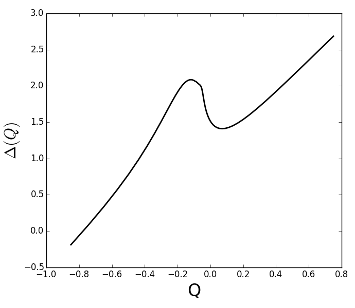
Figure 6: Plot of $\Delta(Q)$ in the VR regime with favorable curvature for higher sound speed, $G_{0}=-0.8,\,b_{0}=0.18$ ($g=G_{0}/b_{0}=-0.44$), showing non-monotonic behavior that arises just after the poles in Fig. 5 coalesce. Unstable complex conjugate roots occur for $\Delta^{\prime}$ just below the local minimum of $\Delta(Q)$.

For $\Delta^{\prime}$ above the relative minimum $\Delta=\Delta_{min}$ in Fig. 6, there are two unstable modes with real $Q$. Just below $\Delta_{min}$, there are complex tearing mode (electromagnetic) roots, and the locus of these roots is similar to that for the RI regime, shown in Fig. 7. In particular, there is a value $\Delta_{crit}>0$, $\Delta_{crit}<\Delta_{min}$ for which the modes with complex roots become stable.

Figure 7: Locus of complex roots in the RI regime with favorable curvature, as $\Delta^{\prime}$ decreases (blue). The black dashed curve is the locus of RI roots for $G_{0}=0$. The marginally stable root encircled in red, with $\omega_{r}<0$, can be Doppler shifted to zero by $v=-\omega_{r}/k$.

The curve $\Delta(Q)$ is nonmonotonic for the wide range $-9.6<g<-1.2$. Below $g=-9.6$, $\Delta(Q)$ becomes monotonic, and becomes a straight line as $g\rightarrow-\infty$. This straight line behavior was observed in Ref. CGJ for very large sound speed and both signs of $D_{s}\propto G_{0}$. From these results it is clear that complex roots for $\Delta^{\prime}<\Delta_{min}$ and stability for $\Delta^{\prime}<\Delta_{crit}$ with $\Delta_{crit}>0$ occurs, as in the RI regime with parallel dynamics. We conclude that the Glasser effect occurs in the VR regime as well, over a wide range of parameters.

For unfavorable curvature ($G_{0}>0$), the symmetry $G_{0}\rightarrow-G_{0}$, $Q\rightarrow-Q$ shows that similar poles occur, but they correspond to growing modes when the roots for $G_{0}<0$ are damped. The last of these poles become complex at $g=1.2$. Past this value, non-monotonic behavior of $\Delta(Q)$, similar to that with favorable curvature and also due to the proximity of the complex electrostatic roots, occurs up to $g=9.6$. However, this non-monotonic behavior is less important for unfavorable curvature, since the electrostatic modes are unstable.

Numerical results for arbitrary balues of $g=G_{0}/b_{0}$ will be presented in a future publication.

IV Resistive wall tearing modes and locking

In this section we present results on error field locking and resistive wall tearing modes, for tearing layers with real frequencies in the plasma frame. For both situations the main effect occurs when the Doppler shift due to the $E\times B$ rotation brings the mode close to zero frequency in the laboratory frame.

IV.1 Resonant field amplification and locking torques

An important consequence of the presence of tearing modes with real frequencies in the plasma frame is related to error field penetration and error field amplification. Recently, a study has been made of the Maxwell torque on a rotating toroidal plasma caused by an error field at rest in the laboratory frame. It was shown FinnColeBrennan that the Maxwell torque on the plasma, applied across the tearing layer, is zero at the velocity for which the frequency of the spontaneous tearing mode in the laboratory frame $\omega_{r}+kv$ is zero, i.e. for $v=-\omega_{r}/k$. (We write the Doppler shift as $\mathbf{k\cdot v}=kv$ because, as discussed below, the poloidal rotation is small. Also, the torque is only exactly zero at $v=-\omega_{r}/k$ in the limit $\gamma\rightarrow 0-$, where $\gamma$ is the growth rate of the spontaneous tearing mode.) We know that spontaneous modes have complex conjugate growth rates $\gamma_{c}=\gamma\mp i\omega_{r}$. For such cases the mode with $\omega_{r}<0$ (the ‘backward wave’) has frequency in the laboratory frame $\omega_{r}+kv$ equal to zero for positive $v=-\omega_{r}/k$. The existence of complex conjugate roots implies that the other ‘backward wave’, for $\omega_{r}>0$, has zero frequency in the laboratory frame for $v=-\omega_{r}/k$, which is negative. A related phenomenon is error field amplification or resonant field amplification, i.e. amplification of the reconnected flux $\tilde{\psi}$ at the tearing layer relative to the magnitude of the error field. This quantity is large when the spontaneous tearing mode is weakly damped, but is maximized when the above condition $v=\pm\omega_{r}/k$ holds. (Again, this is the exact velocity of the peak in reconnected flux only in the limit $\gamma\rightarrow 0-$.) These conclusions imply that the reconnected flux is symmetric with respect to $v$. As we will discuss later, other tearing modes do not have complex conjugate roots, so that this symmetry is not present.

As in Ref. FinnColeBrennan , we expand $\psi(r)=\alpha_{1}\phi_{1}(r)+\alpha_{2}\phi_{2}(r)$, where $\phi_{1}(r_{w})=0$ and $\phi_{2}(r_{t})=0$; here $\phi_{1}$ is the flux for the ideal wall tearing mode and $\phi_{2}$ is the flux to the right of the mode rational surface at $r_{t}$ allowing for the error field at the wall, at $r_{w}$. Using the constant-$\psi$ approximation, the reconnected flux ar $r=r_{t}$ is found to be

$$\psi(r_{t})=\frac{l_{21}}{\Delta(ikv)-\Delta_{1}}\tilde{\psi}(r_{w}),$$ (33)

where $l_{21}=\phi_{2}^{\prime}(r_{t}+)$, $\tilde{\psi}(r_{w})$ is the error field, $\Delta_{1}=[\tilde{\psi}^{\prime}]_{r_{t}}$ and $\Delta(\gamma)$, used here with $\gamma\rightarrow ikv$, is the dispersion quantity discussed in Secs. II and III, and $\Omega=\mathbf{k\cdot v}$ is the Doppler shift. The denominator $\Delta-\Delta_{1}$ vanishes when the ideal wall (spontaneous) tearing mode dispersion relation is satisfied. The reconnected flux has peaks near marginal stability $\gamma\lesssim 0$ and, for spontaneous modes with real frequencies, when $kv=\pm\omega$. Except for the inclusion of pressure-curvature terms in $\Delta(Q)$, these layer calculations can be perfomed in slab geometry.

The Maxwell force on the tearing layer $\int\tilde{j}_{||}\tilde{B}_{x}dV$ is given by ColeFinnHegnaTerry

$$F_{m}=-\frac{k_{x}}{2}\text{Im}(\Delta(ikv))|\tilde{\psi}(r_{t})|^{2}$$

$$=-\frac{k_{x}}{2}\text{Im}(\Delta(ikv))\frac{l_{21}^{2}}{|\Delta(ikv)-\Delta_{1}|^{2}}|\tilde{\psi}(r_{w})|^{2}.$$ (34)

In toroidal geometry, the force in the poloidal direction is dominated by magnetic pumping, so that, as mentioned above, this leads to essentially zero poloidal rotation, giving $\mathbf{k\cdot v}=kv$. The toroidal force is the quantity in Eq. (34), as usual reduced by the factor $-r_{t}/q(r_{t})R$, and the associated torque is $N_{m}=RF_{m}$, where $R$ is the major radius.

The reconnected flux and Maxwell torque for real frequency tearing modes in the RI regime with pressure and field line curvature $D\sim p^{\prime}\kappa$ (Glasser effect) were studied in Ref. FinnColeBrennan . In Fig. 8a we show the reconnected flux for the VR regime with $D<0$. The quantity $Q_{0}$ is defined below. In Fig. 8b we show the Maxwell force (or torque) and the viscous torque, due to an external source of momentum and plasma viscosityFinnColeBrennan . The qualitative behavior is as in Ref. FinnColeBrennan . Specifically, there are three ranges of parameters: one for which there is only a locked state, one for which there is only an unlocked state, and a third in which there are three possible states, with only the locked and unlocked states stable. Because the torque $N_{m}=RF_{m}$ increases sharply, the locked state is just to the right of $v=-\omega_{r}/k$. Furthermore, the velocity of the locked state asymptotes to this value as the error field $\tilde{\psi}(r_{w})$ goes to infinity, i.e. as $N_{m}\sim|\tilde{\psi}(r_{w})|^{2}\rightarrow\infty$. Also, as in Ref. FinnColeBrennan , we find that there are two other possible states with negative velocities, and only the one with more negative velocity is stable. Notice the symmetry for $v\rightarrow-v$ in the reconnected flux and the antisymmetry in the torque. We will return to the issue of other regimes without these symmetry properties.

For computing torques for slightly damped spontaneous modes, there is another complication: the presence of the denominators $Q^{2}+b^{2}\xi^{2}\sim-\omega^{2}+k_{||}^{2}c_{s}^{2}$ (sound wave propagators) in Eq. (31) lead to sound wave resonances and continuum-like effects because the equations for $\tilde{p}$ and $\tilde{v}_{||}$, Eqs. (15) and (16), have no dissipation. This resonance is on the imaginary $Q$ axis so that slightly damped modes are close to this continuum. This continuum can be moved to the left in the complex $Q$ plane by $Q\rightarrow Q+Q_{0}$ in the sound wave propagators, i.e. by including drag terms either Eq. (15) or Eq. (16) or both. The inclusion of perpendicular resistivity in Eq. (16) increases the order of the equations and has the much more profound effect of removing this sound continuum. Details will be presented in a future publication. Interestingly, in the RI regime with pressure gradient and curvature, this continuum (for $Q_{0}=0$) is along the rays $Q\propto e^{\pm 2\pi i/3}$ with $Q_{r}<0$ (except for $Q_{i}=0$, $Q_{r}=0$). This property follows from the fact that $\omega^{2}-k_{||}^{2}c_{s}^{2}=0$ has $Q^{2}\sim-b_{0}^{2}Q^{1/2}$ for $\xi^{2}\sim 1$.

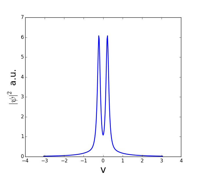
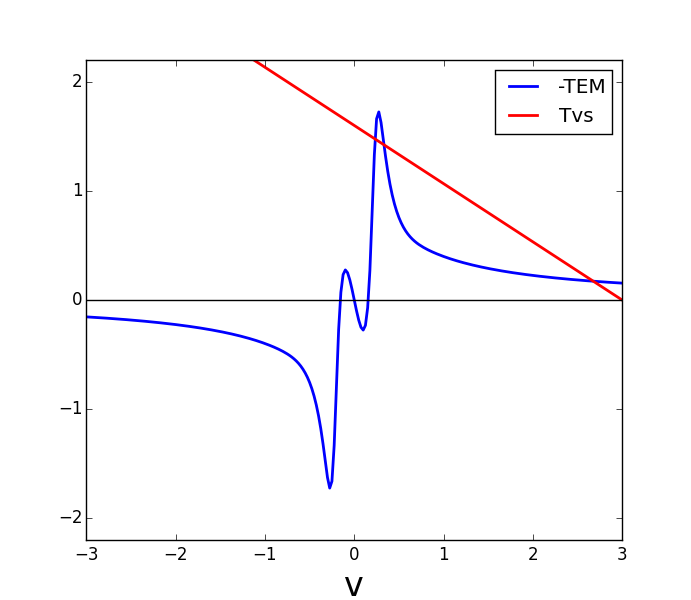
Figure 8: Reconnected flux $|\psi|^{2}$ (a) and torques $N_{m}$ (labeled TEM) (b) for the VR Glasser regime, for a case with a slightly damped spontaneous tearing mode, with $G_{0}=-0.8,\,b_{0}=0.18$, and for drag coefficient $Q_{0}=0.05$. The intersecting viscous torque $T_{vs}$ is also shown in (b). The peaks in $|\psi|^{2}$ coincide approximately with $v=\pm\omega_{r}/k$, as do the zeroes of the torque $N_{m}$ away from $v=0$. The leftmost intersection with the viscous torque line is just above $v=\omega_{r}/k$.

The results in the RI regime and in the VR regime, both with $D<0$, have the property discussed above that modes with complex growth rates occur in complex conjugate pairs $\gamma_{c}=\gamma\pm i\omega_{r}$, leading to the symmetries apparent in Fig. 8. Such symmetries may not hold in other regimes with real frequencies, e.g. when $\omega_{r}$ is due to electron diamagnetism, so that spontaneous modes have $\omega_{r}\sim\omega_{*}$, the diamagnetic frequency (drift-tearing modes.)

IV.2 Resistive wall tearing modes with real frequency tearing layers

A closely related issue is that of resistive wall tearing modes, in which the tearing layers have real frequencies. First, let us review the situation without real frequencies. In the case of VR layers without pressure, the ideal wall tearing modes have real $\gamma$ for stable as well as unstable modes, as discussed in Ref. FinnGerwinModeCoupling . This is easily seen by an analysis as in Sec. IV.1. We use $\gamma\tau_{vr}\tilde{\psi}(r_{t})=[\tilde{\psi}^{\prime}]_{r_{t}}$, i.e. the constant-$\psi$ VR relation for the tearing layer and $\gamma\tau_{w}\tilde{\psi}(r_{w})=[\tilde{\psi}^{\prime}]_{r_{w}}$, the thin-wall (constant-$\psi$) relation for the resistive wall. By methods as in Sec. IV.1 we find

$$\left[\begin{array}[]{cc}\Delta_{1}-\gamma\tau_{vr}&l_{21}\\ l_{12}&\Delta_{2}-\gamma\tau_{w}\end{array}\right]\left(\begin{array}[]{c}\alpha_{1}\\ \alpha_{2}\end{array}\right)=\left[\begin{array}[]{cc}D_{1}(\gamma)&l_{21}\\ l_{12}&D_{2}(\gamma)\end{array}\right]\left(\begin{array}[]{c}\alpha_{1}\\ \alpha_{2}\end{array}\right)=0,$$ (35)

where again $l_{21}=\phi_{2}^{\prime}(r_{t}+)$, $\Delta_{1}=[\phi_{1}^{\prime}]_{r_{t}}$. We have used $D_{1}(\gamma)=\Delta_{1}-\Delta(\gamma)=\Delta_{1}-\gamma\tau_{vr}$, The quantity $\Delta_{1}$ determines the stability of the ideal wall tearing mode ($\tau_{w}=\infty$); it depends on the current profile and also on the pressure profile. We also have $l_{12}=-\phi_{1}^{\prime}(r_{w}-)$ and $\Delta_{2}=[\phi_{2}^{\prime}]_{r_{w}}$. Both $l_{21}$ and $l_{12}$ are positive. The quantity $\Delta_{2}$ depends on the location of a second, conducting, wall at $r_{c}>r_{w}$. The possibility $r_{c}=\infty$ is allowed, and $\Delta_{2}$ determines the stability of the ideal plasma resistive wall mode ($\tau_{vr}=\infty$).

Plasma $E\times B$ rotation is included by letting $\gamma\rightarrow\gamma+i\Omega$, where $\Omega=kv(r_{t})$. We can compute the critical value for $\Delta_{1}$ (critical value of $\beta$, where the pressure gradient-curvature drive comes from the ideal outer region) for which the more unstable mode is marginally stable. As discussed in Ref. FinnGerwinModeCoupling , this critical value always increases with $\Omega$ for the VR model. The interpretation of this result is that the two uncoupled modes in the presence of rotation, with $\gamma=\Delta_{1}/\tau_{vr}-i\Omega$ and $\gamma=\Delta_{2}/\tau_{w}$, are closest in the complex plane for $\Omega=0$, and therefore are coupled most strongly there. The Doppler shift, for $\Omega$ positive or negative, only suppresses the flux from penetrating the wall. Thus, rotation is always stabilizing for the VR model.

In the RI regime, again without pressure, these results are modified by $\gamma\tau_{vr}\rightarrow(\gamma\tau_{ri})^{5/4}$. As also discussed in Ref. FinnGerwinModeCoupling , the critical $\Delta_{1}$ (critical $\beta$) decreases slightly for small $\Omega$, followed by an increase. This is also explained by the mode coupling picture: the uncoupled modes, with $\gamma=\Delta_{1}^{4/5}/\tau_{ri}-i\Omega$ and $\gamma=\Delta_{2}/\tau_{w}$, are closest for negative $\Delta_{1}$ when $\Omega$ equals $-\omega_{r}$, the imaginary part of $\Delta_{1}^{4/5}/\tau_{ri}$, namely $=\pm|\Delta_{1}|^{4/5}\sin(4\pi i/5)\tau_{ri}$. Therefore the strongest coupling is for either of these values of $\Omega$, and further increases in $|\Omega|$ are stabilizing. Again, the strongest destabilizing effect is for that value of $\Omega$ for which one of the real frequencies is Doppler shifted to have zero phase velocity in the laboratory frame. However, as discussed in Ref. FinnGerwinModeCoupling , this effect is very weak for the RI regime without pressure, because $|\omega_{r}|$ becomes appreciable only when the growth rate $|\Delta_{1}|^{4/5}\cos(4\pi i/5)\tau_{ri}$ becomes strongly negative. (On the other hand, it was found FinnGerwinModeCoupling that ideal plasma resistive wall modes, with purely real frequencies for stable modes, can be strongly destabilized over a wide range of rotation values. )

For tearing mode regimes in which there is a nonzero value of real frequency near marginal stability, as discussed in Secs. II.2 and III.2, the effect of rotation on the resistive wall tearing mode is much more significant that it is in the RI regime in Ref. FinnGerwinModeCoupling . This effect is most pronounced if the ideal wall tearing mode is very weakly damped. These results are also explained by the mode coupling picture of Ref. FinnGerwinModeCoupling .

We have found similar results for resistive wall tearing modes with layers in the VR regime with pressure. These effects are due to the real frequencies (Glasser effect) found in this regime, as shown in Sec. III.2. These results are qualitatively different from those in Ref. FinnGerwinModeCoupling , in which the resistive wall tearing mode in the VR regime without pressure was shown to be stabilized for any value of $\Omega$.

There is an interesting application to double tearing modes, of interest in reversed shear profiles. If such a mode has both layers in the VR regime, the mode is described by Eq. (35), with $\tau_{vr}\rightarrow\tau_{vr1}$ and $\tau_{w}\rightarrow\tau_{vr2}$. That is, a second tearing layer in the VR regime acts like a resistive wall. In this formalism, the two single tearing modes (e.g. in the VR regime), with $\gamma\tau_{vr1}=\Delta_{1}$ ($\alpha_{2}=0$, e.g. $\tau_{vr2}=\infty$) and $\gamma\tau_{vr2}=\Delta_{2}$ ($\alpha_{1}=0$, e.g. $\tau_{vr1}=\infty$) are coupled by $l_{12}l_{21}$, giving a double tearing mode which is more unstable than either single tearing mode. The formulation of Eq. (35) shows that relative rotation of the two resonant surfaces only stabilizes this double tearing mode with layers in the VR regime. If, on the other hand one or both layes are in regimes with real frequencies, $\gamma\tau_{vr1}\rightarrow D_{1}(\gamma)$ or $\gamma\tau_{vr2}\rightarrow D_{2}(\gamma)$, then the situation becomes identical to that studied in this section for resistive wall modes. A finite value of the relative rotation of the two layers can destabilize, leading to a maximum growth rate very near where $\omega_{r1}+kv(r_{1})$ equals $\omega_{r2}+kv(r_{2})$. That is, sheared rotation (i.e. different rotation rates at the two rational surfaces) can destabilize double tearing modes. Finally, a similar effect can occur in coupling of the $m$ and $m\pm 1$ poloidal Fourier harmonics in toroidal geometry. These points will be expanded upon in a future publication.

V Summary and discussion

We have first re-analyzed the tearing mode in the RI regime in the presence of pressure gradient and favorable or unfavorable field line curvature in the tearing layer, with parallel dynamics. For unfavorable curvature the dispersion relation $\Delta^{\prime}=\Delta(Q)$ on the real $Q$ axis ($Q$ is the dimensionless, possibly complex, growth rate) has poles, corresponding to unstable electrostatic resistive interchanges. As the sound speed increases, these poles disappear from the real $Q$ axis at $Q=0$. For large enough sound speed the dispersion relation has the known form GGJ1 ; GGJ2 ; FinnManheimer $\Delta(Q)=C_{1}Q^{5/4}-C_{2}/Q^{1/4}$, with $C_{2}$ proportional to the pressure gradient. The behavior $\Delta(Q)\propto-Q^{-1/4}$ for unfavorable curvature as $Q\rightarrow 0$ appears to be a remnant of the last electrostatic pole that disappears into $Q=0$. For favorable curvature (change in sign of $p^{\prime}(r)$ or toroidal effects for $q>1$), $\Delta(Q)$ also has this form, with $C_{2}\rightarrow-C_{2}$, and the poles corresponding to electrostatic modes are in the complex plane, and so do not show up on the positive or negative real $Q$ axis. This calculation does not include the divergence of the $E\times B$ drift or perpendicular resistivity $\eta_{\perp}$ (resistive particle flux) included in the early treatments, and shows that these effects are not important for the qualitative behavior that is evident from this dispersion relation. This behavior includes the occurrence of complex roots $Q$ for $\Delta^{\prime}<\Delta_{min}$ and the stabilization of these roots for $\Delta^{\prime}<\Delta_{crit}$, with $0<\Delta_{crit}<\Delta_{min}$. The analysis is aided by the use of the layer symmetry in the RI regime, namely $p^{\prime}\rightarrow\nu^{3/2}p^{\prime},\,\,c_{s}\rightarrow\nu^{3/4}c_{s},\,\,\gamma\rightarrow\nu\gamma$. In Appendix A we argue that the effects of the divergence of the $E\times B$ drift and the perpendicular resistivity $\eta_{\perp}$ are comparable in magnitude to the other terms kept; results including these effects will be included in a future publication. Another point of this analysis is to illustrate the simple methods that can be employed in the absence of these last two effects, and to explore further the connection between the electrostatic resistive interchanges and the non-monotonic behavior of $\Delta(Q)$ that is responsible for the complex roots.

We have also treated the tearing mode in the VR regime with pressure gradient and parallel dynamics, again neglecting the divergence of the $E\times B$ drift and the perpendicular resistivity. The methods employed are the same as those used in the RI regime. We again find electrostatic resistive interchanges which cause poles in $\Delta(Q)$, on the positive real axis for unfavorable curvature and on the negative real axis for favorable curvature. These calculations are aided by the symmetry $p^{\prime}\rightarrow\lambda p^{\prime},\,\,\gamma\rightarrow\lambda\gamma$ and $c_{s}\rightarrow\lambda c_{s}$, for real (not only positive) $\lambda$. As the sound speed is increased, the poles of $\Delta^{\prime}=\Delta(Q)$ on the real axis corresponding to these resistive interchanges move to $Q=0$ and disappear into the complex plane, except for the last two. For favorable curvature, these coalesce at negative real $Q$ to form complex conjugate poles with $Q_{r}<0$ rather than disappearing from the real $Q$ axis into $Q=0$ as in the RI regime. For higher sound speed, the presence of these last two complex electrostatic resistive interchange roots is responsible for non-monotonic behavior of $\Delta(Q)$, with a relative minimum $\Delta_{min}$. For $\Delta^{\prime}$ below $\Delta_{min}$, the tearing mode dispersion relation $\Delta^{\prime}=\Delta(Q)$ has complex roots. As $\Delta^{\prime}$ is lowered further in this range, these modes with complex frequency are stabilized at $\Delta^{\prime}=\Delta_{crit}$, where $0<\Delta_{crit}<\Delta_{min}$. That is, there is a Glasser effect, with real frequencies as well as stabilization for positive $\Delta^{\prime}$, in the VR regime. This non-monotonic behavior exists over a large range in sound speed.

Tearing modes in two fluid models, including diamagnetic effects, also typically have real frequencies of order the diamagnetic frequency, $\omega_{r}\sim\omega_{*}$, with a reduction in growth rate $\gamma$ Coppi-1 ; Coppi-2 ; Biskamp ; FMA ; ColeFitzpatrick2 . Real frequencies also occur in tearing modes driven by parallel velocity shear Finn-vparallel-prime . Based on these regimes and the new finite frequency results in the VR regime in this paper, we can say with confidence that tearing modes with real frequencies are the rule rather than the exception in most tearing mode regimes. These frequencies are of course in the plasma frame; in the laboratory frame these linear modes have an additional Doppler shift due to $E\times B$ plasma rotation, which is typically diamagnetic in magnitude.

As we have discussed, these real frequencies are responsible for newly discovered results related to resonant field amplification of error fields FinnColeBrennan and for a major modification of error field penetration or locking FinnColeBrennan , allowing locking to just above a finite value of rotation rather than to just above zero rotation. These effects are related to the behavior of resistive wall modes for real frequency tearing modes. In Ref. FinnGerwinModeCoupling it was argued that the ideal plasma resistive wall mode is described as a mode coupling between the plasma mode and the leakage of flux through the resistive wall. This mode is driven unstable by $E\times B$ rotation, specifically lowering the critical $\beta$ for instability, because the plasma rotation Doppler shifts the real frequency stable ideal plasma mode to have small real frequency in the laboratory frame. A similar, but very weak, destabilization effect was shown in Ref. FinnGerwinModeCoupling for tearing modes in the RI regime with no pressure-curvature drive in the layer. It was also shown that no such destabilization effect occurs for VR tearing modes without pressure-curvature drive in the layer, because these modes are purely growing or purely damped, independent of the sign of $\Delta^{\prime}$, in the plasma frame. In this paper we presented a formulation for the study of resistive wall tearing modes with pressure gradient and field line curvature in either the RI or VR regime. As we discussed in an earlier section, the modes with parallel dynamics have real frequency layers in the plasma frame in both of these regimes. We have shown a simple model of mode coupling between an ideal wall tearing mode and an ideal plasma resistive wall mode in the presence of drive by pressure and curvature in the outer region. We showed that the most unstable mode is strongly destabilized by slow $E\times B$ rotation for $\beta$ below the no-wall tearing mode $\beta$ limit, but stabilized for larger rotation. Also, we found that the destabilizing effect is maximized when the ideal wall tearing mode has nearly zero frequency in the laboratory frame, $\omega_{r}+kv\approx 0$, maximizing the coupling of the ideal wall tearing mode and the ideal plasma resistive wall mode.

We have noted a straightforward extension of the resistive wall tearing results of this paper: We considered double tearing modes with either or both tearing layers having real frequency layers. Similar considerations to those pertaining to resistive wall tearing modes suggest a maximum growth rate at the crossing $\omega_{r1}+kv(r_{1})=\omega_{r2}+kv(r_{2})$. Such results show that rotation shear, specifically a difference in plasma rotation between the two mode rational surfaces, can destabilize double tearing modes. Similar considerations apply to poloidal coupling in toroidal geometry.

Acknowledgments. The work of J. M. Finn was supported by the DOE Office of Science, Fusion Energy Sciences and performed under the auspices of the NNSA of the U.S. DOE by LANL, operated by LANS LLC under Contract No DEAC52-06NA25396. The work of A. J. Cole and D. P. Brennan was supported by the DOE Office of Science collaborative Grant Nos. DE-SC0014119 and DE-SC0014005, respectively.

Appendix A. Divergence of the $E\times B$ velocity and perpendicular resistivity

The perturbed perpendicular $E\times B$ flow is $\tilde{\mathbf{v}}_{\perp}=-\nabla\tilde{\Phi}_{es}\times\hat{\mathbf{b}}/B(r)$, where $\tilde{\Phi}_{es}=-B(r)\tilde{\phi}$ is the perturbed electrostatic potential. In this extension of reduced MHD, we allow $\hat{\mathbf{b}}$ and $\hat{\mathbf{z}}$ to differ and neither $B_{z}(r)$ nor $B(r)$ is exactly constant. The divergence of $\tilde{\mathbf{v}}_{\perp}$ takes the form

$$\nabla\cdot\tilde{\mathbf{v}}_{\perp}\approx 2\hat{\mathbf{b}}\times\mathbf{\boldsymbol{\boldsymbol{\kappa}}}\cdot\nabla\tilde{\Phi}_{es}/B\approx-2\nabla\tilde{\phi}\times\hat{\mathbf{z}}\cdot\mathbf{\boldsymbol{\boldsymbol{\kappa}}}.$$

The equation for the pressure takes the form

$$\gamma\tilde{p}+\nabla\tilde{\phi}\times\hat{\mathbf{z}}\cdot\left(\nabla p-2\Gamma p\boldsymbol{\mathbf{\boldsymbol{\kappa}}}\right)=0$$

plus parallel dynamics, so that Eq. (15) of Sec. II.2 has

$$p^{\prime}(r)\rightarrow p^{\prime}(r)-2\Gamma p\kappa,$$

effectively lowering the pressure gradient in Eq. (15). Note that the pressure gradient term in Eq. (16) is unaffected. We see that the pressure gradient term from Eq. (15) and the $\nabla\cdot\tilde{\mathbf{v}}_{\perp}$ term are in the ratio

$$\frac{r_{t}p^{\prime}(r_{t})}{\Gamma p}\,\,:\,\,\frac{2B_{\theta}^{2}}{B_{0}^{2}}.$$

We conclude that the $\nabla\cdot\tilde{\mathbf{v}}_{\perp}$ term, although it is stabilizing, is small in the cylindrical tokamak limit, with $B_{\theta}/B\sim r_{t}/R$. (In the RI regime, these two terms are proportional to the terms in the expression $S-2D_{s}/\Gamma\beta$ of Refs. CGJ ; FinnManheimer , in reverse order, and note that these two terms are comparable if $B_{\theta}\sim B_{z}$, as in an RFP.) In Sec. II.2, in taking $g=G_{0}/b_{0}^{2}$ small, we must not violate this assumption.

Including $\eta_{\perp}\mathbf{j}_{\perp}$ in Ohm’s law in the equations in the tearing layer, we find

$$\tilde{\mathbf{v}}_{\perp}=-\frac{\nabla\tilde{\Phi}_{es}\times\hat{\mathbf{b}}}{B^{2}}-\eta_{\perp}\frac{\mathbf{\tilde{j}}\times\mathbf{B}}{B^{2}}.$$

The last term, which approximately equals $-\eta_{\perp}\nabla\tilde{p}/B^{2}$; $n\tilde{\mathbf{v}}_{\perp}$, is the flux responsible for classical diffusion (without the Pfirsch Schlüter correction). The leading correction enters the adiabatic law via $\Gamma p\nabla\cdot\tilde{\mathbf{v}}_{\perp}$ and equals $-\eta_{\perp}\Gamma p\nabla^{2}\tilde{p}/B_{0}^{2}=-\eta_{\perp}(\Gamma p/B_{0}^{2})\tilde{p}^{\prime\prime}$. To compare its magnitude, we must compare

$$\gamma\,\,:\,\,\frac{\eta_{\perp}\beta}{\delta^{2}}.$$ (36)

From the RI regime ordering of Sec. II, with $\delta\sim\epsilon$, $\gamma\sim\epsilon^{3/2}$, $\eta_{\perp}\sim\eta_{||}\sim\epsilon^{5/2}$ and $\beta\sim\epsilon$ the terms in Eq. (36) compare as

$$\epsilon^{3/2}\,\,:\,\,\epsilon^{3/2}.$$

That is, the dominant term proportional to $\eta_{\perp}$ is comparable to the other terms. Let us consider this same comparison in the VR regime. Assuming $\delta\sim\epsilon,\,\,\gamma\sim\epsilon^{2},\,\,\eta_{\perp}\sim\eta_{||}\sim\epsilon^{3}$ and $\beta\sim\epsilon$ as in Sec. III,the terms in Eq. (36) scale as

$$\epsilon^{2}\,\,:\,\,\epsilon^{2}.$$

Nevertheless, in either tearing regime it is not inconsistent to ignore this $\eta_{\perp}$ term, which introduces complexity by increasing the order of the equations, and the results of Sec. II.2 show that the reglect of the $\eta_{\perp}$ term (as well as the neglect of the $\nabla\cdot\tilde{\mathbf{v}}_{\perp}$ term) do not make any qualitative difference in the RI regime with pressure-curvature drive.

References

- [1] N. Aiba and M. Hirota. Excitation of flow-stabilized resistive wall mode by coupling with stable eigenmodes in tokamaks. Physical Review Letters, 114:065001, 2015.
- [2] D. Biskamp. Drift-tearing modes in a tokamak plasma. Nucl. Fusion, 18:1059, 1978.
- [3] A. Cole, J. Finn, C. Hegna, and P. Terry. Forces and moments within layers of driven tearing modes with sheared rotation. Phys. Plasmas, 22:102514, 2015.
- [4] A. J. Cole and R. Fitzpatrick. Drift-magnetohydrodynamical model of error-field penetration in tokamak plasmas. Phys. Plasmas, 13:032503, 2006.
- [5] B. Coppi. Influence of gyration radius and collisions on hydromagnetic stability (Larmor ion gyro-radius and collision effect on MHD stability of low pressure equilibrium configurations based on Fokker-Planck equation). Phys. Fluids, 7:1501, 1964.
- [6] B. Coppi. Current driven instabilities in configurations with sheared magnetic fields. Phys. Fluids, 8:2273, 1965.
- [7] B. Coppi, J. M. Greene, and J. L. Johnson. Resistive instabilities in a diffuse linear pinch. Nucl. Fusion, 6:101, 1966.
- [8] J. M. Finn. New parallel velocity shear instability. Phys. Plasmas, 2:4400, 1995.
- [9] J. M. Finn, A. J. Cole, and D. P. Brennan. Error field penetration and locking to the backward propagating wave. Phys. Plasmas (Letters), 22:120701, 2015.
- [10] J. M. Finn and R. A. Gerwin. Mode coupling effects on resistive wall instabilities. Phys. Plasmas, 3:2344, 1996.
- [11] J. M. Finn and W. M. Manheimer. Resistive interchange modes in reversed-field pinches. Phys. Fluids, 25:697, 1982.
- [12] J. M. Finn, W. M. Manheimer, and T. M. Antonsen. Drift-resistive interchange and tearing modes in cylindrical geometry. Phys. Fluids, 26:962, 1983.
- [13] A. H. Glasser, J. M. Greene, and J. L. Johnson. Resistive instabilities in general toroidal plasma configurations. Phys. Fluids, 18:875, 1975.
- [14] A. H. Glasser, John M. Greene, and J. L. Johnson. Resistive instabilities in a tokamak. Phys. Fluids, 19:567, 1976.