Refined mass-critical Strichartz estimates for Schrödinger operators

Abstract.

We develop refined Strichartz estimates at $L^{2}$ regularity for a class of time-dependent Schrödinger operators. Such refinements quantify near-optimizers of the Strichartz estimate, and play a pivotal part in the global theory of mass-critical NLS. On one hand, the harmonic analysis is quite subtle in the $L^{2}$-critical setting due to an enormous group of symmetries, while on the other hand, the spacetime Fourier analysis employed by the existing approaches to the constant-coefficient equation are not adapted to nontranslation-invariant situations, especially with potentials as large as those considered in this article.

Using phase space techniques, we reduce to proving certain analogues of (adjoint) bilinear Fourier restriction estimates. Then we extend Tao’s bilinear restriction estimate for paraboloids to more general Schrödinger operators. As a particular application, the resulting inverse Strichartz theorem and profile decompositions constitute a key harmonic analysis input for studying large data solutions to the $L^{2}$-critical NLS with a harmonic oscillator potential in dimensions $\geq 2$. This article builds on recent work of Killip, Visan, and the author in one space dimension.

1. Introduction

In this article, we prove sharpened forms of the Strichartz inequality for nontranslation-invariant linear Schrödinger equations with $L^{2}$ initial data. Recall that solutions to the linear constant-coefficient Schrödinger equation

(1) $$i\partial_{t}u=-\frac{1}{2}\Delta u,\quad u(0,\cdot)=u_{0}\in L^{2}(\mathbf{R}^{d}),$$

satisfy the Strichartz inequality [Str77]

(2) $$\|u\|_{L^{\frac{2(d+2)}{d}}_{t,x}(\mathbf{R}\times\mathbf{R}^{d})}\leq C\|u(0,\cdot)\|_{L^{2}(\mathbf{R}^{d})}.$$

On the other hand, it is also known if $u$ a solution that comes close to saturating this inequality, then it must exhibit some “concentration”; see [CK07, MV98, MVV99, BV07]. Such inverse theorems may be equivalently formulated as a refined estimate

(3) $$\|u\|_{L^{\frac{2(d+2)}{d}}_{t,x}}\lesssim\|u\|_{X}^{\theta}\|u(0,\cdot)\|_{L^{2}(\mathbf{R}^{d})}^{1-\theta},$$

where the norm $X$ is weaker than the right side of (2) but measures the “microlocal concentration” of the solution. We pursue analogues of such refinements when the right side of (1) is replaced by a more general Schrödinger operator $-\tfrac{1}{2}\Delta+V(t,x)$.

Inverse theorems for the Strichartz inequality have provided a key input to the study of the $L^{2}$-critical NLS

(4) $$i\partial_{t}u=-\frac{1}{2}\Delta u\pm|u|^{\frac{4}{d}}u,\quad u(0,\cdot)\in L^{2}(\mathbf{R}^{d}),$$

so termed because the rescaling $u\mapsto u_{\lambda}(t,x):=\lambda^{d/2}u(\lambda^{2}t,\lambda x)$ preserves both the equation (1) and the $L^{2}$-norm $M[u]:=\|u(t)\|_{L^{2}(\mathbf{R}^{d})}=\|u(0)\|_{L^{2}(\mathbf{R}^{d})}$. Indeed, they are used to construct the profile decompositions underpinning the Bourgain-Kenig-Merle concentration compactness and rigidity method by identifying potential blowup scenarios for nonlinear solutions with large data. Using this method, the large data global regularity problem for (4) was recently settled by Dodson [Dod16a, Dod16b, Dod12, Dod15], building on earlier work of Killip, Visan, Tao, and Zhang [KTV09, KVZ08, TVZ07]. For further discussion of this equation we refer the interested reader to the lecture notes [KV13].

The large group of symmetries for the inequality (2) is a significant obstruction to characterizing its near-optimizers. Besides translation and scaling symmetry, both sides are also invariant under Galilei transformations

$$u\mapsto u_{\xi_{0}}(t,x):=e^{i[\langle x,\xi_{0}\rangle-\frac{1}{2}t|\xi_{0}|^{2}]}u(t,x-t\xi_{0}),\quad\xi_{0}\in\mathbf{R}^{d}.$$

This last symmetry emerges only at $L^{2}$ regularity and creates an additional layer of complexity. In particular, while the Littlewood-Paley decomposition is extremely well-adapted to higher Sobolev regularity variants of (2), such as the $\dot{H}^{1}$-critical estimate

$$\|u\|_{L^{\frac{2(d+2)}{d-2}}_{t,x}}\lesssim\|\nabla u(0)\|_{L^{2}(\mathbf{R}^{d})},$$

it is useless for inverting the $L^{2}$-critical estimate because one has no a priori knowledge of where the solution is concentrated in frequency. Instead, the mass-critical refinements cited above combine spacetime Fourier-analytic arguments with restriction theory for the paraboloid.

In physical applications, one is naturally led to consider variants of the mass-critical equation (4) with external potentials, such as the harmonic oscillator

(5) $$i\partial_{t}u=\Bigl{(}-\frac{1}{2}\Delta+\sum_{j}\omega_{j}^{2}x_{j}^{2}\Bigr{)}u\pm|u|^{\frac{4}{d}}u,\quad u(0,\cdot)\in L^{2}(\mathbf{R}^{d}).$$

For instance, the cubic equation (with a $|u|^{2}u$ nonlinearity) has been proposed as a model for Bose-Einstein condensates in a laboratory trap [Zha00] where $\|u(t)\|_{L^{2}}$ represents the total number of particles, and in two space dimensions the critical Sobolev norm for this equation is precisely $L^{2}$.

While introducing the potential breaks scaling symmetry, one nonetheless expects solutions with highly concentrated initial data to be approximated, for short times, by solutions to the scale-invariant equation (4). Less obviously, the equation is invariant under “generalized” Galilei boosts, detailed in Lemma 1.1 below, where the spatial and frequency parameters act together on the solutions; in the constant coefficient setting, this reduces to the usual independent space translation and Galilei boost symmetries.

This article develops refined Strichartz estimates for the linear equation

$$i\partial_{t}u=\Bigl{(}-\frac{1}{2}\Delta+V\Bigr{)}u,\quad u(0,\cdot)\in L^{2}(\mathbf{R}^{d}),$$

for a class $\mathcal{V}$ of real-valued potentials $V(t,x)$ that merely satisfy similar bounds as the harmonic oscillator and possibly also depend on time. Specifically, define

(6) $$\mathcal{V}:=\{V:\mathbf{R}\times\mathbf{R}^{d}\to\mathbf{R}:\|\partial^{\alpha}_{x}V\|_{L^{\infty}_{t,x}}\leq M_{|\alpha|}\text{ for }2\leq|\alpha|\leq N=N(d).\}$$

for fixed constants $0<M_{1},M_{2},\dots,M_{N}$. These estimates play a key role in the large data theory for nontranslation-invariant $L^{2}$-critical Cauchy problems typified by (5). We briefly discuss the nonlinear problem in the last section of the introduction.

The case of one space dimension was treated in a previous joint work with Killip and Visan [JKV]. This paper extends the methods introduced there to higher dimensions.

1.1. The setup

To clarify the structure of our arguments we begin with a slightly more general setup. Hence we consider time-dependent, real-valued symbols $a(t,x,\xi)$ which are measurable in $t$ and satisfy

(7) $$|\partial^{\alpha}_{x}\partial^{\beta}_{\xi}a|\leq c_{\alpha\beta}\ \text{for all}\ |\alpha|+|\beta|\geq 2.$$

Further, we assume the characteristic curvature condition

(8) $$\bigl{|}|\operatorname{det}a_{\xi\xi}|-1\bigr{|}+\bigl{|}\|a_{\xi\xi}\|-1\bigr{|}\leq\varepsilon$$

for some small $0<\varepsilon<1$. For concreteness, all matrix norms in this article denote the Hilbert-Schmidt norm, but the exact choice of norm is inessential.

These hypotheses encompass several interesting situations:

• Schrödinger Hamiltonians with time-dependent scalar potentials $a=\tfrac{1}{2}|\xi|^{2}+V(t,x)$, where $V\in\mathcal{V}$.

• Electromagnetic-type symbols $a=\tfrac{1}{2}|\xi|^{2}+b(x,\xi)+V(t,x)$, where the first order symbol $b(x,\xi)$ is real and satisfies $|\partial^{\alpha}_{x}\partial^{\beta}_{\xi}b|\leq c_{\alpha\beta}$ for all $|\alpha|+|\beta|\geq 1$, and $V\in\mathcal{V}$ is a scalar potential as before.

• The frequency $1$ portion of the Laplacian on a curved background.

For a symbol as defined above, write $a^{w}(t,x,D)$ for its Weyl quantization. Let $U(t,s)$ denote its unitary propagator on $L^{2}(\mathbf{R}^{d})$, so that $u:=U(t,s)u_{s}$ is the solution to the equation

(9) $$(D_{t}+a^{w}(t,x,D))u=0,\quad u(s,\cdot)=u_{s}\in L^{2}(\mathbf{R}^{d}),$$

Evolution equations of this type were studied by Koch and Tataru [KT05]. While translations and modulations do not preserve the equation (9), they do preserve the class of equations defined by our assumptions. For an element $(x_{0},\xi_{0})$ of classical phase space, define the “phase space translation” operator $\pi(x_{0},\xi_{0})$ by

$$\pi(z_{0})f(x)=e^{i\langle x-x_{0},\xi_{0}\rangle}f(x-x_{0}).$$

Then a direct computation, as in the proof of [KT05, Proposition 4.3], yields

Lemma 1.1.

If $U(t,s)$ is the propagator for the symbol $a$ and $\sigma\mapsto z^{\sigma}=(x^{\sigma},\xi^{\sigma})$ is a bicharacteristic of $a$, then

$$U(t,s)\pi(z_{0}^{s})f=e^{i(\phi(t,z_{0})-\phi(s,z_{0}))}\pi(z_{0}^{t})U^{z_{0}}(t,s),$$

where $U^{z_{0}}$ is the propagator for the equation

$$[D_{t}+(a^{z_{0}})^{w}(t,x,D)]u=0,$$

$$a^{z_{0}}(t,z)=a(t,z_{0}^{t}+z)-\langle x,a_{x}(t,z_{0}^{t})\rangle-\langle\xi,a_{\xi}(t,z_{0}^{t})\rangle-a(z_{0}^{t}),$$

and the phase is defined by

$$\phi(t,z_{0})=\int_{0}^{t}\langle a_{\xi}(\tau,z_{0}^{\tau}),\xi_{0}^{\tau}\rangle-a(\tau,z_{0}^{\tau})\,d\tau.$$

Observe that the transformed symbol $a^{z_{0}}$ satisfies the same estimates assumed of $a$. As a special case, symbols of the form $a=\tfrac{1}{2}|\xi|^{2}+\langle A(t,x),\xi\rangle+\omega_{jk}(t)x^{j}x^{k}$ are themselves preserved by the mapping $a\mapsto a^{z_{0}}$ if $A=A_{j}dx^{j}$ is a 1-form whose components are linear functions of the space variables with time-dependent coefficients. In two and three space dimensions, such $A$ are potentials for uniform magnetic fields.

The preceding hypotheses imply that the equation (9) satisfies a local-in-time dispersive estimate:

Lemma 1.2.

If the symbol $a$ satisfies the conditions (7) and 8, there exists $T_{0}>0$ such that the propagator $U(t,s)$ for the evolution equation (9) satisfies the estimate

(10) $$\|U(t,s)\|_{L^{1}_{x}\to L^{\infty}_{x}}\lesssim|t-s|^{-d/2}\ \text{for all}\ |t-s|\leq T_{0}.$$

Hence, the solutions to (9) satisfy local-in-time Strichartz estimates

$$\|u\|_{L^{q}_{t}L^{r}_{x}(I\times\mathbf{R}^{d})}\lesssim_{|I|}\|u_{s}\|_{L^{2}(\mathbf{R}^{d})}$$

for any compact time interval $I$, and for all Strichartz exponents $(q,r)$ satisfying $2\leq q,r\leq\infty$, $\tfrac{2}{q}+\tfrac{d}{r}=\tfrac{d}{2}$, and $(q,r,d)\neq(2,\infty,2)$.

Proof sketch.

The dispersive estimate is shown in Koch-Tataru using wavepacket parametrices [KT05, Proposition 4.7]. Standard arguments (see Ginibre-Velo [GV95] and Keel-Tao [KT98]) then yield the Strichartz estimates. ∎

It suffices to choose the time increment $T_{0}$ so that

(11) $$T_{0}\leq 1,\quad T_{0}\|a_{x\xi}\|+T_{0}^{2}\|a_{xx}\|\leq\eta,$$

where $\eta=\eta(d)$ is a small parameter depending only on the dimension.

Remark.

The concrete cases of scalar potentials and magnetic potentials were studied much earlier by Fujiwara and Yajima, respectively, who proved the dispersive bound using Fourier integral parametrices [Fuj79, Yaj91].

We seek refinements of the Strichartz inequality analogous to those for the constant-coefficient equation. The earlier arguments for constant coefficient equation relied crucially on subtle bilinear estimates from Fourier restriction theory. We isolate and reformulate the technical lynchpin in the present context.

Hypothesis 1.

There exist $T_{0}>0$ and $1<p<\tfrac{d+2}{d}$ such that the following holds: if $f,g\in L^{2}(\mathbf{R}^{d})$ have frequency supports in sets of diameter $\lesssim N$ which are separated by distance $\sim N$, then

(12) $$\|U_{\lambda}^{s}(t)fU_{\lambda}^{s}(t)g\|_{L^{p}_{t,x}([-T_{0},T_{0}]\times\mathbf{R}^{d})}\lesssim N^{-\delta}\|f\|_{L^{2}(\mathbf{R}^{d})}\|g\|_{L^{2}(\mathbf{R}^{d})},$$

for all $s\in[-1,1]$ and all $0<\lambda\leq 1$, where $U_{\lambda}^{s}(t)=U^{s}_{\lambda}(t,0)$ are the propagators for the time-translated and rescaled symbols $a^{s}_{\lambda}:=\lambda^{2}a(s+\lambda^{2}t,\lambda x,\lambda^{-1}\xi)$.

When $a=\tfrac{1}{2}|\xi|^{2}$, the scaling and translation parameters $\lambda,\ s$ are extraneous, and inequalities of the form (12) are called (adjoint) bilinear Fourier restriction estimates. They were utilized by Bégout-Vargas to obtain mass-critical Strichartz refinements in dimension $3$ and higher [BV07] (the results in dimensions 1 and 2, due to Carles-Keraani, Merle-Vega, and Moyua-Vargas-Vega utilized linear restriction estimates [CK07, MV98, MVV99]). For further discussion of such estimates see for instance [Tao03] and the references therein.

In the first part of this paper, we connect (12) to Strichartz refinements. To measure concentration in the solution we test it against scaled, modulated, and translated wavepackets. Set

(13) $$\psi(x)=c_{d}e^{-\frac{|x|^{2}}{2}},\ \psi_{x_{0},\xi_{0}}=\pi(x_{0},\xi_{0})\psi,\quad c_{d}=2^{-d/2}\pi^{-3d/4},$$

where $S_{\lambda}$ is the the unitary rescaling $S_{\lambda}f(x):=\lambda^{-d/2}f(\lambda^{-1}x)$.

Theorem 1.3.

If Hypothesis 1 holds, then there exists $0<\theta<1$ such that for all initial data $u_{0}\in L^{2}(\mathbf{R}^{d})$, the solution $u$ to the equation (9) satisfies

(14) $$\|u\|_{L^{\frac{2(d+2)}{d}}([-1,1]\times\mathbf{R}^{d})}\lesssim\bigl{(}\sup_{0<\lambda\leq 1,\ |t|\leq 1,\ (x_{0},\xi_{0})\in T^{*}\mathbf{R}^{d}}|\langle S_{\lambda}\psi_{x_{0},\xi_{0}},u(t)\rangle_{L^{2}(\mathbf{R}^{d})}|\bigr{)}^{\theta}\|u_{0}\|_{L^{2}(\mathbf{R}^{d})}^{1-\theta}.$$

The generality of our hypotheses requires us to formulate the estimates locally in time. Indeed, for most potentials the left side of the Strichartz estimate (14) is infinite if one integrates over $\mathbf{R}\times\mathbf{R}^{d}$; for instance, the harmonic oscillator potential $V=|x|^{2}$ admits periodic-in-time solutions. Nonetheless, our methods do yield (a new proof of) a global-in-time refined Strichartz estimate

$$\|u\|_{L^{\frac{2(d+2)}{d}}_{t,x}(\mathbf{R}\times\mathbf{R}^{d})}\lesssim\Bigl{(}\sup_{\lambda>0,\ t\in\mathbf{R},\ (x_{0},\xi_{0})\in T^{*}\mathbf{R}^{d}}|\langle S_{\lambda}\psi_{x_{0},\xi_{0}},u(t)\rangle_{L^{2}(\mathbf{R}^{d})}|\Bigr{)}^{\theta}\|u_{0}\|_{L^{2}(\mathbf{R}^{d})}^{1-\theta}.$$

for solutions to the constant coefficient equation (1).

In applications to PDE, such a refined estimate is nowadays interpreted in the framework of concentration compactness, and yields profile decompositions via repeated application of the following

Lemma 1.4.

Assume the estimate (14) holds. Let $u_{n}:=U(t)f_{n}$ be a sequence of linear solutions with initial data $u_{n}(0)=f_{n}\in L^{2}(\mathbf{R}^{d})$ such that $\|f_{n}\|_{L^{2}(\mathbf{R}^{d})}\leq A<\infty$ and $\|u_{n}\|_{L^{\frac{2(d+2)}{d}}_{t,x}}\geq\varepsilon>0$. Then, after passing to a subsequence, there exist parameters

$$\{(\lambda_{n},t_{n},x_{n},\xi_{n})\}_{n}\subset(0,1]\times[-1,1]\times\mathbf{R}^{d}_{x}\times\mathbf{R}^{d}_{\xi}$$

and a function $0\neq\phi\in L^{2}(\mathbf{R}^{d})$ such that

$$\pi(x_{n},\xi_{n})^{-1}S_{\lambda_{n}}^{-1}u_{n}\rightharpoonup\phi\ \text{in}\ L^{2}$$

$$\|\phi\|_{L^{2}}\gtrsim\varepsilon\Bigl{(}\frac{\varepsilon}{A}\Bigr{)}^{\frac{1-\theta}{\theta}}.$$

Further,

$$\|f_{n}\|_{L^{2}}^{2}-\|f_{n}-U(t_{n})^{-1}S_{\lambda_{n}}\pi(x_{n},\xi_{n})S_{\lambda_{n}}\phi\|_{L^{2}}^{2}-\|U(t_{n})^{-1}S_{\lambda_{n}}\pi(x_{n},\xi_{n})S_{\lambda_{n}}\phi\|_{L^{2}}^{2}\to 0.$$

Proof.

By the estimate (14), there exist $\lambda_{n},t_{n},x_{n},\xi_{n}$ such that

$$|\langle S_{\lambda_{n}}\psi_{x_{n},\xi_{n}},U(t_{n})f_{n}\rangle|=|\langle\psi,\pi(x_{n},\xi_{n})^{-1}S_{\lambda_{n}}^{-1}U(t_{n})f_{n}\rangle|\gtrsim\varepsilon\Bigl{(}\frac{\varepsilon}{A}\Bigr{)}^{\frac{1-\theta}{\theta}}.$$

The sequence $\pi(x_{n},\xi_{n})^{-1}S_{\lambda_{n}}^{-1}U(t_{n})f_{n}$ is bounded in $L^{2}$, and therefore converges weakly in $L^{2}$ to some $\phi$ after passing to a subsequence. The lower bound on $\|\phi\|_{L^{2}}$ is immediate, while

$$\|f_{n}\|_{L^{2}}^{2}-\|f_{n}-U(t_{n})^{-1}S_{\lambda_{n}}\pi(x_{n},\xi_{n})\phi\|_{L^{2}}^{2}-\|U(t_{n})^{-1}S_{\lambda_{n}}\pi(x_{n},\xi_{n})\phi\|_{L^{2}}^{2}$$

$$=2\operatorname{Re}\langle f_{n}-U(t_{n})^{-1}S_{\lambda_{n}}\pi(x_{n},\xi_{n})\phi,U(t_{n})^{-1}S_{\lambda_{n}}\pi(x_{n},\xi_{n})\phi\rangle$$

$$=2\operatorname{Re}\langle\pi(x_{n},\xi_{n})^{-1}S_{\lambda_{n}}^{-1}U(t_{n})f_{n}-\phi,\phi\rangle\to 0.$$

∎

Further discussion of profile decompositions and inverse Strichartz theorems may be found in the lecture notes [KV13] and the references therein.

In the second part of this paper, we verify Hypothesis 1 for scalar potentials.

Theorem 1.5.

Consider a Schrödinger operator of the form $H(t)=-\tfrac{1}{2}\Delta+V(t,x)$, where $V\in\mathcal{V}$. Suppose $S_{1},S_{2}\subset\mathbf{R}^{d}_{\xi}$ are subsets of Fourier space with $\operatorname{diam}(S_{j})\leq N$ and $c^{-1}N\geq\operatorname{dist}(S_{1},S_{2})\geq cN$ for some $0<c<1$. There exists a constant $\eta=\eta(c)>0$ such that if $\tau_{0}>0$ satisfies

$$(\tau_{0}+\tau_{0}^{2})\|\partial^{2}_{x}V\|_{L^{\infty}}<\eta,$$

then for any $f,g\in L^{2}(\mathbf{R}^{d})$ with $\operatorname{supp}(\hat{f})\subset S_{1}$ and $\operatorname{supp}(\hat{g})\subset S_{2}$, the corresponding linear solutions $u=U(t,0)f$ and $v=U(t,0)g$ satisfy the estimate

(15) $$\|uv\|_{L^{q}([-T_{0},T_{0}]\times\mathbf{R}^{d})}\lesssim_{\varepsilon}N^{d-\frac{d+2}{q}+\varepsilon}\|f\|_{L^{2}}\|g\|_{L^{2}}\quad\text{for all}\quad\frac{d+3}{d+1}\leq q<\frac{d+2}{d}$$

for any $\varepsilon>0$, $N\geq 1$, and $V\in\mathcal{V}$.

For $V=0$, the above estimate was conjectured by Klainerman and Machedon without the epsilon loss, and first proved by Wolff for the wave equation [Wol01] and subsequently by Tao [Tao03] for the Schrödinger equation (both with the epsilon loss). Strictly speaking, the time truncation is not present in the original formulations of those estimates, but may be easily removed by a rescaling and limiting argument.

Finally, while we make no attempt to address general magnetic potentials, a simple case with some physical relevance does essentially follow from the proof for scalar potentials. The necessary modifications for the following theorem are sketched in the last section.

Theorem 1.6.

The conclusion of the previous theorem holds for Schrödinger operators of the form $H(t)=-\tfrac{1}{2}(\nabla-iA)^{2}+V(t,x)$ where $A=A_{j}dx^{j}$ is a 1-form whose components are linear in the space variables (i.e. the vector potential for a uniform magnetic field), and condition on the time increment $\tau_{0}$ is replaced by

$$\tau_{0}\|a_{x\xi}\|+(\tau_{0}+\tau_{0}^{2})\|a_{xx}\|<\eta.$$

We remark that the restriction estimate (12) does not hold for all symbols satisfying the conditions (7) and (8). For instance, it was observed by Vargas [Var05] that when $U(t)=e^{it\partial_{x}\partial_{y}}$ is the “nonelliptic” Schrödinger propagator in two space dimensions (thus $a=\xi_{x}\xi_{y}$), the bilinear restriction estimate (7) can fail unless the frequency supports of the two inputs are not only disjoint but also separated in both Fourier coordinates. In fact, the refinement (14) as stated is false for the nonelliptic equation; for a correct formulation, one should enlarge the symmetry group on the right side to include the hyperbolic rescalings $u(x,y)\mapsto u(\mu x,\mu^{-1}y)$; see the work of Rogers and Vargas [RV06].

While the classical bicharacteristics of elliptic and nonelliptic propagators seemingly have no qualitative difference—and indeed the dispersive estimates hold equally well for both—the quantum propagators have radically different behavior in terms of oscillations in time. If one compares the travelling wave solutions

$$e^{i[x\xi_{x}+y\xi_{y}-\frac{t}{2}(\xi_{x}^{2}+\xi_{y}^{2})]},\quad e^{i[x\xi_{x}+y\xi_{y}-t\xi_{x}\xi_{y}]},$$

it is evident that unlike in the elliptic case, two solutions to the nonelliptic equation which are well-separated in spatial frequency need not decouple in time.

The lesson of this counterexample is that while the dispersive and Strichartz estimates follow directly from properties of the classical Hamiltonian flow, an inverse Strichartz estimate depends more subtly on the temporal oscillations of the quantum evolution, which is connected to the bilinear decoupling estimates.

1.2. The main ideas

Suppose one has initial data $u_{0}\in L^{2}$ such that the corresponding solution $u$ has nontrivial Strichartz norm. Then, we need to identify a bubble of concentration in $u$, characterized by several parameters that reflect the underlying symmetries in the problem. In the $L^{2}$-critical setting, the relevant features consist of a significant length scale $\lambda_{0}$ as well as the position $x_{0}$, frequency $\xi_{0}$, and time $t_{0}$ when concentration occurs.

The existing proofs of Strichartz refinements for the constant-coefficient equation first use spacetime Fourier analysis (including restriction estimates) to identify a cube $Q$ in Fourier space accounting for a significant portion of the spacetime norm of $u$, which reveals the frequency center $\xi_{0}$ and scale $\lambda_{0}$ of the concentration. For example, Begout-Vargas [BV07] first establish an extimate of the form

$$\|e^{\frac{it\Delta}{2}}f\|_{L^{\frac{2(d+2)}{d}}}\lesssim\Bigl{(}\sup_{Q\ \text{dyadic cubes}}|Q|^{1-\frac{p}{2}}\int_{Q}|\hat{f}(\xi)|^{p}\,d\xi\Bigr{)}^{\mu}\|f\|_{L^{2}(\mathbf{R}^{d})}^{1-\mu p}$$

Then, the time $t_{0}$ and position $x_{0}$ are recovered via a separate physical-space argument. These arguments ultimately rely on the fact that when $V=0$, the equation is diagonalized by the Fourier transform.

For equations with variable coefficients, it is more natural to consider position $x_{0}$ and frequency $\xi_{0}$ together as a point in phase space, which propagates along the bicharacteristics for the equation. Following the approach in [JKV] for the one-dimensional equation, we work in the physical space and first isolate a significant time interval $[t_{0}-\lambda_{0}^{2},t_{0}+\lambda_{0}^{2}]$, which also suggests a characteristic scale $\lambda_{0}$. Then $x_{0}$ and $\xi_{0}$ are recovered by phase space techniques.

The first part of the argument in [JKV] carries over essentially unchanged; however, the ensuing phase space analysis in higher dimensions is more involved and occupies the bulk of this article.

1.3. An application to mass-critical NLS

This article was originally motivated by the problem of proving global wellposedness for the mass-critical quantum harmonic oscillator

(16) $$i\partial_{t}u=\Bigl{(}-\frac{1}{2}\Delta+\sum_{j}\omega_{j}^{2}x_{j}^{2}\Bigr{)}u\pm|u|^{\frac{4}{d}}u.$$

By spectral theory, the Cauchy problem for (16) is naturally posed in the “harmonic” Sobolev spaces

$$u_{0}\in\mathcal{H}^{s}:=\{u_{0}\in L^{2}:(-\Delta+\sum_{j}\omega_{j}^{2}|x|^{2})^{s/2},\ u_{0}\in L^{2}\}$$

Global existence for data in the “energy” space $\mathcal{H}^{1}$ was studied by Zhang [Zha05]. More recently, Poiret, Robert, and Thomann established probabilistic wellposedness in two space dimensions for all subcritical cases $0<s<1$, as well as for other supercritical problems [PRT14]. Another recent contribution by Burq, Thomann, and Tzvetkov constructs Gibbs measures and proves probabilistic global wellposedness for the critical case in one dimension [BTT13].

It is well-known that the isotropic harmonic oscillator $\omega_{j}\equiv\tfrac{1}{2}$ may be “trivially” solved; to construct solutions on unit length time intervals for arbitrary $L^{2}$ data, it suffices to observe that $u$ is a solution of (4) on $\mathbf{R}_{t}\times\mathbf{R}_{x}^{d}$ iff its Lens transform

$$\mathcal{L}u(t,x):=\frac{1}{(\cos t)^{d/2}}u\Bigl{(}\tan t,\frac{x}{\cos t}\Bigr{)}e^{-\frac{i|x|^{2}\tan t}{2}}$$

solves (16) on $(-\pi/2\times\pi/2)_{t}\times\mathbf{R}_{x}^{d}$ with the same initial data. However, this trick relies on algebraic cancellations that no longer hold for more general harmonic oscillators. For further discussion of the nonlinear harmonic oscillator as well as its connection with the Lens transform, consult the article of Carles [Car11].

To solve (16) for large data in the critical space $L^{2}$, the concentration compactness and rigidity approach is much more promising. Experience has shown that constructing suitable profile decompositions is a core difficulty implementing this strategy for dispersive equations with broken symmetries (e.g. loss of translation-invariance). For instance, see [Jao16] for the energy-critical variant of the quantum harmonic oscillator, as well as [IPS12, KVZ], and the references therein, for other energy-critical NLS on non-Euclidean domains. Thus this article supplies the main harmonic analysis input for the deterministic large data theory of (16) at the critical regularity.

Acknowledgements. The author is grateful to Michael Christ, Rowan Killip, Daniel Tataru, and Monica Visan for many helpful discussions, and also wishes to thank the anonymous referee for numerous suggestions for improving the original manuscript. This research was partially supported by the National Science Foundation under Award No. 1604623. Part of this work was completed during the 2017 Oberwolfach workshop in “Nonlinear Waves and Dispersive Equations.”

2. Preliminaries

2.1. Notation

We use the Japanese bracket notation $\langle x\rangle:=(1+|x|^{2})^{\frac{1}{2}}$.

2.2. Classical flow estimates

We collect some elementary properties of the classical Hamiltonian flow

(19) $$\left\{\begin{array}[]{ll}\dot{x}=a_{\xi},&x(0)=y\\ \dot{\xi}=-a_{x},&\xi(0)=\eta.\end{array}\right.$$

Solutions to this system are bicharacteristics. For a point $z=(x,\xi)$ in phase space, let $\sigma\mapsto z^{\sigma}=(x^{\sigma},\xi^{\sigma})$ denote the bicharacteristic initialized at $(x,\xi)$. Write $(y,\eta)\mapsto(x^{t}(y,\eta),\xi^{t}(y,\eta))$ for the flow map.

The linearization of (19) satisfies the following Gronwall estimates:

Lemma 2.1.

Suppose $|t|\|\partial_{x,\xi}^{2}a\|_{L^{\infty}}\leq 1$. Then

(20) $$\begin{split}\frac{\partial x^{t}}{\partial\eta}&=\int_{0}^{t}a_{\xi\xi}(\tau,x^{\tau},\xi^{\tau})\,d\tau+O(t^{2}\|a_{x\xi}\|a_{\xi\xi}\|)+O(t^{3}\|a_{xx}\|\|a_{\xi\xi}\|^{2})\\ \frac{\partial\xi^{t}}{\partial\eta}&=I+O(t\|a_{\xi x}\|)+O(t^{2}\|a_{xx}\|\|a_{\xi\xi}\|)\\ \frac{\partial x^{t}}{\partial y}&=I+O(t\|a_{x\xi}\|)+O(t^{2}\|a_{xx}\|\|a_{\xi\xi}\|)\\ \frac{\partial\xi^{t}}{\partial y}&=\int_{0}^{t}-a_{xx}(\tau,x^{\tau},\xi^{\tau})\,d\tau+O(t^{2}\|a_{xx}\|\|a_{x\xi}\|)+O(t^{3}\|a_{xx}\|^{2}\|a_{\xi\xi}\|)\end{split}.$$

Proof.

The linearized system takes the form

$$\dot{y} =a_{\xi x}y+a_{\xi\xi}\eta,$$

$$\dot{\eta} =-a_{xx}y-a_{x\xi}\eta.$$

A preliminary application of Gronwall implies $|y(t)|+|\eta(t)|\lesssim|y(0)|+|\eta(0)|$.

Consider initial data $y(0)=I,\ \eta(0)=0$. Then

$$|\eta(t)|\leq\int_{0}^{t}|a_{xx}y|\,d\tau+\int_{0}^{t}|a_{x\xi}\eta(\tau)|\,d\tau,$$

so $|\eta(t)|\lesssim t\|a_{xx}\|.$ Substituting this into the equation for $y$, we deduce

$$|y-I|\leq\int_{0}^{t}|a_{\xi x}y|\,d\tau+\int_{0}^{t}|a_{\xi\xi}\eta|\,d\tau\lesssim t\|a_{\xi x}\|+t^{2}\|a_{\xi\xi}\|\|a_{xx}\|.$$

This in turn yields the refinement

$$\Bigl{|}\eta(t)+\int_{0}^{t}a_{xx}\,d\tau\Bigr{|}\lesssim t^{2}\|a_{xx}\|\|a_{\xi x}\|+t^{3}\|a_{xx}\|^{2}\|a_{\xi\xi}\|.$$

The case $y(0)=0,\ \eta(0)=I$ is similar. We have

$$|y(t)|\leq\int_{0}^{t}|a_{\xi\xi}\eta|\,d\tau+\int_{0}^{t}|a_{\xi x}y|\,d\tau\Rightarrow|y(t)|\lesssim t\|a_{\xi\xi}\|,$$

which yields

$$|\eta(t)-I| \lesssim\int_{0}^{t}\|a_{xx}\|\|a_{\xi\xi}\|\tau\,d\tau+\int_{0}^{t}|a_{x\xi}\eta|\,d\tau\lesssim t\|a_{x\xi}\|+t^{2}\|a_{xx}\|\|a_{\xi\xi}\|,$$

$$\Bigl{|}y(t)-\int_{0}^{t}a_{\xi\xi}\,d\tau\Bigr{|} \lesssim t^{2}\|a_{\xi x}\|\|a_{\xi\xi}\|+t^{3}\|a_{xx}\|\|a_{\xi\xi}\|^{2}.$$

∎

These imply, in view of the normalizations (8), the integrated estimates

(21) $$\begin{split}&\begin{split}x^{t}_{1}-x_{2}^{t}&=x_{1}^{s}-x_{2}^{s}+[I^{\prime}+O(\varepsilon)](t-s)(\xi_{1}^{s}-\xi_{2}^{s})\\ &+O(|t-s|\|a_{x\xi}\|)(|x_{1}^{s}-x_{2}^{s}|+|t-s||\xi_{1}^{s}-\xi_{2}^{s}|)\\ &+O(|t-s|^{2}\|a_{xx}\|)(|x_{1}^{s}-x_{2}^{s}|)+|t-s||\xi_{1}^{s}-\xi_{2}^{s}|).\end{split}\\ &\begin{split}\xi_{1}^{t}-\xi_{2}^{t}&=\xi_{1}^{s}-\xi_{2}^{s}\\ &+O(|t-s|\|a_{xx}\|)|x_{1}^{s}-x_{2}^{s}|\\ &+O(|t-s|^{2}\|a_{xx}\|\|a_{x\xi}\|)|x_{1}^{s}-x_{2}^{s}|+O(|t-s|\|a_{x\xi}\|)|\xi_{1}^{s}-\xi_{2}^{s}|\\ &+O(|t-s|^{3}\|a_{xx}\|^{2})|x_{1}^{s}-x_{2}^{s}|+O(|t-s|^{2}\|a_{xx}\|)|\xi_{1}^{s}-\xi_{2}^{s}|,\end{split}\end{split}$$

where $I^{\prime}$ is an orthogonal matrix which equals the identity if $a_{\xi\xi}$ is positive-definite. In particular, we have

Corollary 2.2.

If $|x_{1}^{s}-x_{2}^{s}|\leq r$, then $|x_{1}^{t}-x_{2}^{t}|\geq Cr$ whenever $\tfrac{2Cr}{|\xi_{1}^{s}-\xi_{2}^{s}|}\leq|t-s|\leq T_{0}$.

Physically, this means that two particles colliding with sufficiently large relative velocity will only interact once in the time window of interest.

Next, we record a technical lemma first proved in the 1d case [JKV, Lemma 2.2]. This is used in the proof of Lemma 4.3 below but the computations use the preceding estimates.

Lemma 2.3.

There exists a constant $C=C(\|\partial^{2}a\|)>0$ so that if $Q_{\eta}=(0,\eta)+[-1,1]^{2d}\subset T^{*}\mathbf{R}^{d}$ and $r\geq 1$, then

$$\bigcup_{|t-t_{0}|\leq\min(|\eta|^{-1},1)}\Phi(t)^{-1}(z_{0}^{t}+rQ_{\eta})\subset\Phi(t_{0})^{-1}(z_{0}^{t_{0}}+CrQ_{\eta}).$$

In other words, if the bicharacteristic $z^{t}$ starting at $z\in T^{*}\mathbf{R}^{d}$ passes through the cube $z_{0}^{t}+rQ_{\eta}$ in phase space during some time window $|t-t_{0}|\leq\min(|\eta|^{-1},1)$, then it must lie in the dilate $z_{0}^{t_{0}}+CrQ_{\eta}$ at time $t_{0}$.

Proof.

If $z\in\Phi(t)^{-1}(z_{0}^{t}+rQ_{\eta})$, by definition we have $|x^{t}-x_{0}^{t}|\leq r$ and $|\xi^{t}-\xi_{0}^{t}-\eta|\leq r$. Assuming that $|\eta|\geq 1$, the estimates (21) imply that

$$|x^{t_{0}}-x_{0}^{t_{0}}| \leq r+|\eta|^{-1}(|\eta|+r)$$

$$+O(|\eta|^{-1}\|\partial^{2}a\|)(r+|\eta|^{-1}(|\eta|+r))+O(|\eta|^{-2}\|\partial^{2}a\|)(r+|\eta|^{-1}(|\eta|+r))$$

$$\leq Cr$$

$$|\xi^{t_{0}}-\xi_{0}^{t_{0}}-\eta| \leq r+O(|\eta|^{-1}\|a_{xx}\|)r+(|\eta|^{-2}\|a_{xx}\|\|a_{x\xi}\|)r+O(|\eta|^{-1}\|a_{x\xi}\|)(|\eta|+r)$$

$$+(|\eta|^{-3}\|a_{xx}\|^{2})r+O(|\eta|^{-2}\|a_{xx}|)(|\eta|+r)$$

$$\leq Cr.$$

The case $|\eta|<1$ is similar. ∎

2.3. Wavepackets

Let $R\geq 1$ be a scale and $z_{0}=(x_{0},\xi_{0})$ be a point in phase space. A scale-$R$ wavepacket at $z_{0}$ is a Schwartz function $\phi_{z_{0}}$ such that $\phi_{z_{0}}$ and its Fourier transform $\widehat{\phi_{z_{0}}}$ concentrate in the regions $|x-x_{0}|\leq R^{1/2}$ and $|\xi-\xi_{0}|\leq R^{-1/2}$, respectively:

$$|(R^{1/2}\partial_{x})^{k}\phi_{z_{0}}(x)|\lesssim_{k,N}\Bigl{\langle}\frac{x-x_{0}}{R^{1/2}}\Bigr{\rangle}^{-N},\quad|(R^{-1/2}\partial_{\xi})^{k}\widehat{\phi_{z_{0}}}(\xi)|\lesssim_{k,N}\Bigl{\langle}\frac{\xi-\xi_{0}}{R^{-1/2}}\Bigr{\rangle}^{-N}\quad\forall k,N\geq 0.$$

There are many ways to decompose $L^{2}$ functions into linear combinations of wavepackets. For the first part of this article, it is technically more convenient to use a continuous decomposition. Later on in Section 6.3, we switch to a discrete version which is more common in the restriction theory literature.

In this section we recall a standard continuous wavepacket transform. To keep things simple we work at unit scale since that is all we shall need. For a function $f\in L^{2}(\mathbf{R}^{d})$, its Bargmann transform or FBI transform is the function $Tf\in L^{2}(T^{*}\mathbf{R}^{d})$ defined by

$$Tf(z)=\langle f,\psi_{z}\rangle_{L^{2}(\mathbf{R}^{d})},\quad\psi_{z}=\pi(z)\psi\text{ as in }\eqref{e:gaussian_wp}.$$

The transform satisfies a Plancherel identity $\|Tf\|_{L^{2}(T^{*}\mathbf{R}^{d})}=\|f\|_{L^{2}(\mathbf{R}^{d})}$; dually, for any wavepacket coefficients $F\in L^{2}(T^{*}\mathbf{R}^{d}_{z})$, one has

$$\|T^{*}F\|_{L^{2}_{x}}=\Big{\|}\int_{T^{*}\mathbf{R}^{d}}F(z)\psi_{z}\,dz\Bigr{\|}_{L^{2}_{x}}\leq\|F\|_{L^{2}_{z}}.$$

Indeed, $TT^{*}$ is the orthogonal projection onto $TL^{2}(\mathbf{R}^{d})$. Then as $T^{*}T=I$, any $f\in L^{2}(\mathbf{R}^{d})$ can be resolved (nonuniquely) into a continuous superposition of wavepackets

$$f(x)=\int_{T^{*}\mathbf{R}^{d}}f_{z}\psi_{z}(x)\,dz.$$

Applying the propagator $U(t)$ to both sides and using linearity and the next lemma, one obtains a wavepacket decomposition

$$u(t,x)=\int u_{z}(t,x)\,dz,\ u_{z}(t,x)=f_{z}[U(t)\psi_{z}](x)$$

of Schrödinger solutions. For brevity we sometimes omit the arguments and write $f=\int f_{z}\,dz,\ u=\int u_{z}\,dz$.

Lemma 2.4 (Evolution of a packet).

If $\psi_{z_{0}}$ is a scale-$1$ wavepacket, $U(t)$ is the propagator for the equation (9), and $z_{0}\mapsto z_{0}^{t}$ is the bicharacteristic starting at $z_{0}$, then $U(t)\psi_{z_{0}}$ is a scale-$1$ wavepacket concentrated at $z_{0}^{t}$ for all $|t|=O(1)$.

Proof sketch.

Using Lemma 1.1 we reduce to the case $z_{0}=0$ and also ensure that the symbol $a(t,x,\xi)$ vanishes to second order at $(x,\xi)=(0,0)$ in addition to satisfying the bounds (7). Then it suffices to show that propagator $U(t)$ for such symbols maps Schwartz functions to Schwartz functions on unit time scales. This is done using weighted Sobolev estimates as in [KT05, Section 4]. ∎

The term wavepacket shall also refer to spacetime functions of the form $U(t)\psi_{z}$, not just the fixed time slices. Later it will be essential to exploit not just the spacetime localization of wavepackets but also their phase as described in Lemma 1.1.

3. Choosing a length scale

We begin with the following lemma from [JKV, Proposition 3.1], obtained by a variant of the usual $TT^{*}$ derivation of the Strichartz estimates. While that article concerned just Schrödinger operators with scalar potentials, the proof works equally well in the current more general setting.

Proposition 3.1.

Suppose $U(t,s)$ satisfies a local in time dispersive estimate as in Lemma 1.2. Let $(q,r)$ be Strichartz exponents (i.e. satisfying the conditions in that Lemma) with $2<q<\infty$. Assume that $f\in L^{2}(\mathbf{R}^{d})$ satisfies $\|f\|_{L^{2}(\mathbf{R}^{d})}=1$ and

$$\|U(t)f\|_{L^{q}_{t}L^{r}_{x}([-1,1]\times\mathbf{R}^{d})}\geq\varepsilon.$$

Then there is a time interval $J\subset[-1,1]$ such that

$$\|U(t,s)f\|_{L^{q-1}_{t}L^{r}_{x}(J\times\mathbf{R}^{d})}\gtrsim|J|^{\frac{1}{q(q-1)}}\varepsilon^{\frac{q}{q-2}}.$$

Equivalently,

$$\|U(t,s)f\|_{L^{q}L^{r}}\lesssim\Bigl{(}\sup_{J\in[-1,1]}|J|^{-\frac{1}{q(q-1)}}\|U(t,s)f\|_{L^{q-1}_{t}L^{r}_{x}(J\times\mathbf{R}^{d})}\Bigr{)}^{1-\frac{2}{q}}\|f\|_{L^{2}(\mathbf{R}^{d})}^{\frac{2}{q}}.$$

Note that by pigeonholing we may always assume that $|J|\leq T_{0}$, where $T_{0}$ is the time increment selected in (11).

Now let $(q,r)$ be the Strichartz exponents determined by the conditions $\tfrac{2}{q}+\tfrac{d}{r}=\tfrac{d}{2}$ and $q-1=r$. It is easy to see that $2<r<\tfrac{2(d+2)}{d}<q<\infty$.

For each $J=[s-\mu,s+\mu]\subset[-1,1]$, we write

$$U(t,s)f=\Bigl{(}\frac{T_{0}}{\mu}\Bigr{)}^{d/4}\tilde{U}\Bigl{(}\frac{T_{0}}{\mu}(t-s),0\Bigr{)}\tilde{f}\Bigl{(}\sqrt{\frac{T_{0}}{\mu}}x),\quad\tilde{f}=\Bigl{(}\frac{\mu}{T_{0}}\Bigr{)}^{d/4}f\Bigl{(}\sqrt{\frac{\mu}{T_{0}}}x\Bigr{)},$$

where $\tilde{U}(t,s)$ is the propagator for the rescaled equation $(D_{t}+\tilde{a}^{w})\tilde{u}=0$, and

$$\tilde{a}(t,x,\xi):=\frac{\mu}{T_{0}}a\Bigl{(}s+\frac{\mu}{T_{0}}t,\sqrt{\frac{\mu}{T_{0}}}x,\sqrt{\frac{T_{0}}{\mu}}\xi\Bigr{)}.$$

Changing variables, we obtain

$$|J|^{-\frac{1}{q(q-1)}}\|U(t,s)f\|_{L^{q-1}_{t}L^{r}(J\times\mathbf{R}^{d})}=\|\tilde{U}(t)\tilde{f}\|_{L^{q-1}_{t}L^{r}_{x}([-T_{0},T_{0}]\times\mathbf{R}^{d})}.$$

By interpolating with $L^{2}_{t,x}([-T_{0},T_{0}]\times\mathbf{R}^{d})$, which is bounded by unitarity, we see that Theorem 1.3 would follow if we prove that for some $2<q_{0}<\tfrac{2(d+2)}{d}$ and $0<\theta<1$, the scale-1 refined estimate

(22) $$\|U_{\lambda}^{s}(t)f\|_{L^{q_{0}}([-T_{0},T_{0}]\times\mathbf{R}^{d})}\lesssim(\sup_{z}|\langle\psi_{z},f\rangle|)^{\theta}\|f\|_{L^{2}}^{1-\theta}.$$

holds for all $s\in[-1,1],\ 0<\lambda\leq 1$, where the notation $U_{\lambda}^{s}(t)$ is as in Hypothesis 1.

Over the next two sections we establish

Proposition 3.2.

If Hypothesis 1 holds, then so does the estimate (22).

4. A refined bilinear $L^{2}$ estimate

In previous work [JKV], we proved (22) when $d=1$ with $q_{0}=4$ by viewing the inequality as a bilinear $L^{2}$ estimate and exploit orthogonality. Such a direct approach fails in $d\geq 2$ dimensions; since $2<\frac{2(d+2)}{d}\leq 4$, the left side of (22) could well be infinite when $q_{0}=4$. To obtain a refined linear $L^{q_{0}}$ estimate for $q_{0}<\tfrac{2(d+2)}{d}$, we also begin by interpreting it as a refined bilinear $L^{q_{0}/2}$ estimate, but use dyadic decomposition and interpolate between two microlocalized estimates:

• A refined bilinear $L^{2}$ estimate (“refined” in the sense of exhibiting a sup over wavepacket coefficients) with some loss in the frequency separation of the inputs.

• A bilinear $L^{p}$ estimate for some $p<\tfrac{d+2}{d}$ which yields gains in the frequency separation, essentially the content of Hypothesis 1.

This section discusses the former. In the next section we put together the two estimates, and the $L^{p}$ estimate is established in the remainder of the paper.

Proposition 4.1.

Suppose $f=\int f_{z}\psi_{z}\,dz$ and $g=\int g_{z}\psi_{z}\,dz$ are $L^{2}(\mathbf{R}^{d})$ initial data with corresponding Schrödinger evolutions $u=\int u_{z}\,dz$ and $v=\int v_{z}\,dz$, where $u_{z}(t,x)=f_{z}[U(t)\psi_{z}](x)$, $v_{z}(t,x)=g_{z}[U(t)\psi_{z}](x)$. Then

(23) $$\Bigl{\|}\int_{|\xi_{1}-\xi_{2}|\sim N}u_{z_{1}}v_{z_{2}}\,dz_{1}dz_{2}\Bigr{\|}_{L^{2}([-T_{0},T_{0}]\times\mathbf{R}^{d})}\lesssim N^{\alpha}(\sup_{z}|f_{z}|^{1/p^{\prime}}\|f_{z}\|_{L^{2}_{z}}^{1/p})(\sup_{z}|g_{z}|^{1/p^{\prime}}\|g_{z}\|_{L^{2}_{z}}^{1/p})$$

for some $\alpha=\alpha(d)$ and $1<p<2$.

Proof.

Square the left side and expand

$$\int f_{z_{1}}g_{z_{2}}\overline{f_{z_{3}}g_{z_{4}}}K_{N}(z_{1},z_{2},z_{3},z_{4})\,dz_{1}dz_{2}dz_{3}dz_{4},$$

where $K_{N}:=K\chi_{|\xi_{1}-\xi_{2}|\sim N,\ |\xi_{3}-\xi_{4}|\sim N}$, and

$$K(z_{1},z_{2},z_{3},z_{4})=\langle U(t)\psi_{z_{1}}U(t)\psi_{z_{2}},\ U(t)\psi_{z_{3}}U(t)\psi_{z_{4}}\rangle_{L^{2}_{t,x}([-T_{0},T_{0}]\times\mathbf{R}^{d})}.$$

The estimate would follow if we could show that

(24) $$N^{-\alpha}\langle z_{1}-z_{2}\rangle^{\theta}\langle z_{3}-z_{4}\rangle^{\theta}|K_{N}(\vec{z})|\text{ is a bounded operator on }L^{2}_{z_{1},z_{2}}\text{ for some }\theta>0,$$

as Young’s inequality would then imply

$$\Bigl{\|}\int u_{z}\,dz\Bigr{\|}_{L^{4}}^{2} \lesssim\left(\int|f_{z_{1}}g_{z_{2}}|^{2}\langle z_{1}-z_{2}\rangle^{-2\theta}\,dz_{1}dz_{2}\right)^{1/2}\left(\int|f_{z_{3}}g_{z_{4}}|^{2}\langle z_{3}-z_{4}\rangle^{-2\theta}dz_{3}dz_{4}\right)^{1/2}$$

$$\lesssim\sup_{z}|f_{z}|^{2/p^{\prime}}\sup_{z}|g_{z}|^{2/p^{\prime}}\|f\|_{L^{2}}^{2/p}\|g\|_{L^{2}}^{2/p}\quad\text{for some}\quad 1<p<2.$$

In view of the crude bound $|K(\vec{z})|\lesssim\min_{j,k}\langle z_{j}-z_{k}\rangle^{-1}$, which follows simply from the spacetime supports of the wavepackets,  (24) would follow from

Lemma 4.2.

The localized kernel $K_{N}$ satisfies

$$\||K_{N}|^{1-\delta}\|_{L^{2}_{z_{1}z_{2}}\to L^{2}_{z_{3}z_{4}}}\lesssim N^{\alpha},$$

where $\alpha$ is a constant depending only on the dimension.

Proof of Lemma 4.2.

In view of the unit scale spatial localization of the wavepackets and the propagation estimates (21), we may further truncate the kernel to the phase space region

$$R=\{|x_{1}-x_{2}|\leq 4|\xi_{1}-\xi_{2}|,\quad|x_{3}-x_{4}|\leq 4|\xi_{3}-\xi_{4}|\}.$$

For instance, if $|x_{1}^{s}-x_{2}^{s}|\geq 4|\xi_{1}^{s}-\xi_{2}^{s}|$ and $|t-s|\leq T_{0}$ with the parameter $\eta$ in (11) chosen sufficiently small,

$$|x_{1}^{t}-x_{2}^{t}| \geq(1-|t-s|^{2}\|\partial^{2}_{x}V\|_{L^{\infty}}e^{|t-s|^{2}\|\partial^{2}_{x}V\|_{L^{\infty}}})|x_{1}^{s}-x_{2}^{s}|$$

$$-(|t-s|+|t-s|^{3}\|\partial^{2}_{x}V\|_{L^{\infty}}e^{|t-s|^{2}\|\partial^{2}_{x}V\|_{L^{\infty}}})|\xi_{1}^{s}-\xi_{2}^{s}|$$

$$\geq\frac{1}{2}|x_{1}^{s}-x_{2}^{s}|-\frac{3}{2}|t-s||\xi_{1}^{s}-\xi_{2}^{s}|$$

$$\geq\frac{1}{8}|x_{1}^{s}-x_{2}^{s}|,$$

therefore $|K_{N}(1-\chi_{R})|\lesssim_{M}\langle x_{1}-x_{2}\rangle^{-M}\langle x_{3}-x_{4}\rangle^{-M}N^{-M}$ for any $M>0$. Thus it suffices to prove that

$$\|K_{N}\chi_{R}\|_{L^{2}\to L^{2}}\lesssim N^{\alpha}.$$

An estimate of this flavor was proved in the 1d case [JKV]. We shall argue similarly, but the proof is somewhat simpler since we aim for a cruder bound at this stage, completely ignoring temporal oscillations, and defer the more delicate analysis to the bilinear $L^{p}$ estimate.

Partition the $4$-particle phase space $(T^{*}\mathbf{R}^{d})^{4}$ according to the degree of physical interaction between the particles. Let

$$E_{0} =\{\vec{z}\in(T^{*}\mathbf{R}^{d})^{4}:\min_{|t|\leq T_{0}}\max_{j,k}|x_{j}^{t}-x_{k}^{t}|\leq 1\},$$

$$E_{k} =\{\vec{z}\in(T^{*}\mathbf{R}^{d})^{4}:2^{k-1}<\min_{|t|\leq T_{0}}\max_{j,k}|x_{j}^{t}-x_{k}^{t}|\leq 2^{k}\},$$

and decompose the kernel $K_{N}=\sum_{k\geq 0}K_{N}\chi_{E_{k}}$. Then we have the following pointwise bound

(25) $$|K(\vec{z})|\lesssim_{M}2^{-kM}\frac{\langle\xi_{1}^{t(\vec{z})}+\xi_{2}^{t(\vec{z})}-\xi_{3}^{t(\vec{z})}-\xi_{4}^{t(\vec{z})}\rangle^{-M}}{\langle|\xi_{1}^{t(\vec{z})}-\xi_{2}^{t(\vec{z})}|+|\xi_{3}^{t(\vec{z})}-\xi_{4}^{t(\vec{z})}|\rangle},\quad\vec{z}\in E_{k},$$

where $t(\vec{z})$ is a time minimizing the “mutual distance” $\max_{i,j}|x_{i}^{t}-x_{j}^{t}|$. Further, the additional localization to $R$ implies, by the estimates (21), that

$$|\xi_{1}^{t}-\xi_{2}^{t}-(\xi_{1}-\xi_{2})| \lesssim\frac{1}{10}|\xi_{1}-\xi_{2}|$$

$$|\xi_{3}^{t}-\xi_{4}^{t}-(\xi_{3}-\xi_{4})| \lesssim\frac{1}{10}|\xi_{3}-\xi_{4}|$$

for all $|t|\leq T_{0}$. In particular $|\xi_{1}^{t(\vec{z})}-\xi_{2}^{t(\vec{z})}|\sim|\xi_{3}^{t(\vec{z})}-\xi_{4}^{t(\vec{z})}|\sim N$; thus, while the $\xi_{j}^{t}$ may vary rapidly with time if $x_{j}^{t}$ are extremely far from the origin, the relative frequencies retain the same order of magnitude.

Assuming the bound (25) for the moment, we apply Schur’s test to complete the proof of Lemma 4.2. Fix $(z_{3},z_{4})$ belonging to the projection $E_{k}\to T^{*}\mathbf{R}^{d}_{z_{3}}\times T^{*}\mathbf{R}^{d}_{z_{4}}$, define

$$E_{k}(z_{3},z_{4})=\{(z_{1},z_{2}):(z_{1},z_{2},z_{3},z_{4})\in E_{k}\},$$

and let $t_{1}$ be the time minimizing $|x_{3}^{t_{1}}-x_{4}^{t_{1}}|\leq 2^{k}$. For any $(z_{1},z_{2})\in E_{k}(z_{3},z_{4})$, the mutual distance $\max_{j,k}|x_{j}^{t}-x_{k}^{t}|$ between $x_{1}^{t},x_{2}^{t},x_{3}^{t},x_{4}^{t}$ is minimized in the time window

$$I=\{t:|t-t_{1}|\lesssim\min\bigl{(}1,\frac{2^{k}}{|\xi_{3}-\xi_{4}|}\bigr{)}\},$$

as for all other times we have $|x_{3}^{t}-x_{4}^{t}|\gg 2^{k}$ (Corollary 2.2).

We estimate the size of the level sets of $|K|$. For a momentum $\xi\in\mathbf{R}^{d}$, let $Q_{\xi}=(0,\xi)+[-1,1]^{d}\times[-1,1]^{d}\subset T^{*}\mathbf{R}^{d}$ denote the unit phase space box centered at $(0,\xi)$, and write $\Phi^{t}=\Phi(t,0)$ for the propagator on classical phase space relative to time $0$ for the Hamiltonian $h(x,\xi)=\tfrac{1}{2}|\xi|^{2}+V(t,x)$. For $\mu_{1},\mu_{2}\in\mathbf{R}^{d}$, define

$$Z_{\mu_{1},\mu_{2}}=\bigcup_{t\in I}(\Phi^{t}\otimes\Phi^{t})^{-1}\Bigl{(}\frac{z_{3}^{t}+z_{4}^{t}}{2}+2^{k}Q_{\mu_{1}}\Bigr{)}\times\Bigl{(}\frac{z_{3}^{t}+z_{4}^{t}}{2}+2^{k}Q_{\mu_{2}}\Bigr{)}.$$

This set is depicted schematically in Figure 1 when $k=0$, and corresponds to the pairs of wave packets $(z_{1},z_{2})\in E_{m}(z_{3},z_{4})$ with momenta $(\mu_{1},\mu_{2})$ relative to the wavepackets $(z_{3},z_{4})$ at the “collision time” $t(\vec{z})$.

Figure 1. $Z_{\mu_{1},\mu_{2}}$ comprises all $(z_{1},z_{2})$ such that $z_{1}^{t}$ and $z_{2}^{t}$ belong to the depicted phase space boxes for $t$ in the interval I.

We note that $E_{k}(z_{3},z_{4})\subset\bigcup_{\mu_{1},\mu_{2}\in\mathbf{Z}^{d}}Z_{\mu_{1},\mu_{2}}$, and recall the following estimate from the 1d paper, whose proof we reproduce below for convenience:

Lemma 4.3.

(26) $$|Z_{\mu_{1},\mu_{2}}|\lesssim 2^{4dk}\max(1,|\mu_{1},|,|\mu_{2}|)|I|.$$

Proof.

Without loss assume $|\mu_{1}|\geq|\mu_{2}|$. Partition the interval $I$ into subintervals of length $|\mu_{1}|^{-1}$ if $\mu_{1}\neq 0$ and in subintervals of length $1$ if $\mu_{1}=0$. For each $t^{\prime}$ in the partition, Lemma 2.3 implies that for some constant $C>0$ we have

$$\begin{split}\bigcup_{|t-t^{\prime}|\leq\min(1,|\mu_{1}|^{-1})}\Phi(t)^{-1}\Bigl{(}\frac{z_{3}^{t}+z_{4}^{t}}{2}+2^{k}Q_{\mu_{1}}\Bigr{)}&\subset\Phi(t^{\prime})^{-1}\Bigl{(}\frac{z_{3}^{t^{\prime}}+z_{4}^{t^{\prime}}}{2}+C2^{k}Q_{\mu_{1}}\Bigr{)}\\ \bigcup_{|t-t^{\prime}|\leq\min(1,|\mu_{1}|^{-1})}\Phi(t)^{-1}\Bigl{(}\frac{z_{3}^{t}+z_{4}^{t}}{2}+2^{k}Q_{\mu_{2}}\Bigr{)}&\subset\Phi(t^{\prime})^{-1}\Bigl{(}\frac{z_{3}^{t^{\prime}}+z_{4}^{t^{\prime}}}{2}+C2^{k}Q_{\mu_{2}}\Bigr{)},\end{split}$$

and so

$$\begin{split}&\bigcup_{|t-t^{\prime}|\leq\min(1,|\mu_{1}|^{-1})}(\Phi(t)\otimes\Phi(t))^{-1}\Bigl{(}\frac{z_{3}^{t}+z_{4}^{t}}{2}+2^{k}Q_{\mu_{1}}\Bigr{)}\times\Bigl{(}\frac{z_{3}^{t}+z_{4}^{t}}{2}+2^{k}Q_{\mu_{2}}\Bigr{)}\\ &\subset(\Phi(t^{\prime})\otimes\Phi(t^{\prime}))^{-1}\Bigl{(}\frac{z_{3}^{t^{\prime}}+z_{4}^{t^{\prime}}}{2}+C2^{k}Q_{\mu_{1}}\Bigr{)}\times\Bigl{(}\frac{z_{3}^{t^{\prime}}+z_{4}^{t^{\prime}}}{2}+C2^{k}Q_{\mu_{2}}\Bigr{)}.\end{split}$$

By Liouville’s theorem, the right side has measure $O(2^{4dk})$ in $(T^{*}\mathbf{R}^{d})^{2}$. The claim follows by summing over the partition. ∎

For each $(z_{1},z_{2})\in E_{k}(z_{3},z_{4})\cap Z_{\mu_{1},\mu_{2}}$, we have by definition $z_{j}^{t(\vec{z})}\in\tfrac{z_{3}^{t(\vec{z})}+z_{4}^{t(\vec{z})}}{2}+2^{k}Q_{\mu_{j}}$, thus

$$\xi_{1}^{t(\vec{z})}+\xi_{2}^{t(\vec{z})}-\xi_{3}^{t(\vec{z})}-\xi_{4}^{t(\vec{z})}=\mu_{1}+\mu_{2}+O(2^{k})$$

$$\xi_{1}^{t(\vec{z})}-\xi_{2}^{t(\vec{z})}=\mu_{1}-\mu_{2}+O(2^{k})$$

Hence when $(z_{1},z_{2})\in Z_{\mu_{1},\mu_{2}}$, for any $M$ we have

(27) $$|K(\vec{z})|\lesssim_{M}2^{-Mk}\frac{\langle\mu_{1}+\mu_{2}\rangle^{-M}}{\langle|\mu_{1}-\mu_{2}|+|\xi_{3}^{t(\vec{z})}-\xi_{4}^{t(\vec{z})}|\rangle}.$$

To apply Schur’s test, we combine the estimates (26), (27), and evaluate

$$\int|K_{N}(z_{1},z_{2},z_{3},z_{4})|^{1-\delta}\chi_{E_{k}}(\vec{z})\,dz_{1}dz_{2} \leq\sum_{\mu_{1},\mu_{2}\in\mathbf{Z}^{d}}\int_{Z_{\mu_{1},\mu_{2}}}|K_{N}^{1-\delta}\chi_{E_{k}}\,dz_{2}dz_{2}$$

$$\lesssim_{M}2^{-Mk}\sum_{|\mu_{1}-\mu_{2}|\lesssim N+2^{k}}2^{-Mk}\langle\mu_{1}+\mu_{2}\rangle^{-M}$$

$$\lesssim N^{d}2^{-(M-d)k}.$$

For fixed $z_{1},z_{2}$, the integral over $z_{3}$ and $z_{4}$ is estimated the same way. This concludes the proof of Lemma 4.2, modulo some remarks on the crucial pointwise bound (25).

To obtain that estimate, we use Lemma 1.1 to write

$$K(\vec{z}) =\int e^{i\Phi}\prod_{j=1}^{4}U^{z_{j}}(t)\psi(x-x_{j}^{t}),\,dxdt,$$

$$\Phi(t,x;\vec{z}) =\sum_{j}\sigma_{j}\Bigl{[}\langle x-x_{j}^{t},\xi_{j}^{t}\rangle+\phi(t,x_{0},\xi_{0})\Bigr{]}$$

where $\sigma=(+,+,-,-)$, and we denote $\prod_{j}c_{j}:=c_{1}c_{2}\overline{c_{3}}\overline{c_{4}}$.

It is convenient to partition the integral further, writing

$$U^{\vec{z}_{j}}(t)\psi(x-x_{j}^{t})=\sum_{\ell_{j}\geq 0}U^{\vec{z}_{j}}(t)\psi(x-x_{j}^{t})\theta_{\ell_{j}}(x-x_{j}^{t})\bigr{)},$$

where $\sum_{\ell\geq 0}\theta_{\ell}$ is a partition of unity with $\theta_{\ell}$ supported on the dyadic annulus of radius $\sim 2^{\ell}$. For $\vec{z}\in E_{k}$, only the terms

$$K_{\vec{\ell}}(\vec{z}):=\int e^{i\Phi}\prod_{j=1}^{4}U^{z_{j}}(t)\psi(x-x_{j}^{t})\theta_{\ell_{j}}(x-x_{j}^{t})\,dxdt$$

with $\ell^{*}:=\max_{j}\ell_{j}\gtrsim k$ will be nonzero.

By Lemma 2.1, the integral is supported on the spacetime region

$$\{(t,x):|t-t(\vec{z})|\lesssim\min\Bigl{(}1,\frac{2^{\ell^{*}}}{\max_{i,j}|\xi_{i}^{t(\vec{z})}-\xi_{k}^{t(\vec{z})}|}\Bigr{)}\quad\text{and}\quad|x-x_{j}^{t}|\lesssim 2^{\ell_{j}}\},$$

and for all such $t$ we have

$$|x_{j}^{t}-x_{k}^{t}|\lesssim 2^{\ell^{*}},\quad|\xi_{j}^{t}-\xi_{k}^{t}-(\xi_{j}^{t(\vec{z})}-\xi_{k}^{t(\vec{z})})|\lesssim 2^{\ell^{*}}.$$

Integrating by parts in $x$, we may produce as many factors of $|\xi_{1}^{t}+\xi_{2}^{t}-\xi_{3}^{t}-\xi_{4}^{t}|^{-1}$ as desired and freeze $t=t(\vec{z})$ to obtain

$$|K_{\vec{\ell}}(\vec{z})|\lesssim_{M}2^{-\ell^{*}M}\frac{\langle\xi_{1}^{t(\vec{z})}+\xi_{2}^{t(\vec{z})}-\xi_{3}^{t(\vec{z})}-\xi_{4}^{t(\vec{z})}\rangle^{-M}}{\langle|\xi_{1}^{t(\vec{z})}-\xi_{2}^{t(\vec{z})}|+|\xi_{3}^{t(\vec{z})}-\xi_{4}^{t(\vec{z})}|\rangle}\quad\text{for any}\quad M\geq 0,$$

and the bound (25) follows upon summing over $\vec{\ell}$. ∎

This completes the proof of Proposition 4.1. ∎

5. Proof of Theorem 1.3

We prove Proposition 3.2 and hence Theorem 1.3. Begin with a Whitney decomposition of

$$(\mathbf{R}^{d}\times\mathbf{R}^{d})\setminus\{(\xi,\xi):\xi\in\mathbf{R}^{d}\}=\bigcup_{N\in 2^{\mathbf{Z}}}\bigcup_{Q\in\mathcal{Q}_{N}}Q,$$

where $\mathcal{Q}_{N}$ is the set of dyadic cubes in $\mathbf{R}^{d}\times\mathbf{R}^{d}$ with diameter $\sim N$ and distance $\sim N$ to the diagonal. For each $Q\in\mathcal{Q}_{N}$, its characteristic function factorizes $\chi_{N}^{Q}(\xi_{1},\xi_{2})=\chi_{N}^{Q,1}(\xi_{2})\chi^{Q,2}_{N}(\xi_{2})$, where $\chi_{N}^{Q,j}$ are characteristic functions of $d$-dimensional cubes of width $N$. Then we can decompose

$$1(\xi_{1},\xi_{2})=\chi_{0}(\xi_{1},\xi_{2})+\sum_{N\geq 1}\sum_{Q\in\mathcal{Q}_{N}}\chi^{Q,1}_{N}(\xi_{1})\chi^{Q,2}_{N}(\xi_{2}),$$

where $\chi_{0}(\xi_{1},\xi_{2})$ is supported on the set $|\xi_{1}-\xi_{2}|\lesssim 1$.

Now suppose $u$ and $v$ are linear solutions with initial data $f=\int f_{z}\psi_{z}\,dz$ and $g=\int g_{z}\psi_{z}\,dz$, respectively, where $f_{z}=\langle f,\psi_{z}\rangle$ and $g_{z}=\langle g,\psi_{z}\rangle$. Writing $u_{z}=f_{z}U(t)\psi_{z}$, $v_{z}=g_{z}U(t)\psi_{z}$, we deduce as a consequence of Hypothesis 1 that

(28) $$\Bigl{\|}\sum_{Q\in\mathcal{Q}_{N}}\int_{Q}u_{z_{1}}v_{z_{2}}\,dz_{1}dz_{2}\Bigr{\|}_{L^{q}([-T_{0},T_{0}]\times\mathbf{R}^{d})}\lesssim N^{-\delta}\|f_{z}\|_{L^{2}_{z}}\|g_{z}\|_{L^{2}_{z}}.$$

for each $N\geq 1$. Indeed, for each cube $Q$ the integral has a product structure

$$\int_{Q}u_{z_{1}}v_{z_{2}}dz_{1}dz_{2} =\Bigl{(}\int u_{z_{1}}\chi^{Q,1}_{N}(\xi_{1})\,dx_{1}d\xi_{1}\Bigr{)}\Bigl{(}\int v_{z_{2}}\chi^{Q,2}_{N}(\xi_{2})\,dx_{2}d\xi_{2}\Bigr{)}$$

$$=U(t)\Bigl{[}\int f_{z_{1}}\chi_{N}^{Q,1}(\xi_{1})\psi_{z_{1}}\,dx_{1}d\xi_{1}\Bigr{]}U(t)\Bigl{[}\int g_{z_{2}}\chi_{N}^{Q,1}(\xi_{2})\psi_{z_{2}}\,dx_{2}d\xi_{2}\Bigr{]}.$$

By the rapid decay of the wavepackets, we may harmlessly insert frequency cutoffs $\tilde{\chi}_{N}^{Q,j}(D)$, where $\tilde{\chi}_{N}^{Q,j}$ are slightly fattened versions of $\chi_{N}^{Q,j}$ and still have supports separated by distance $\sim N$, and apply Hypothesis 1 to estimate

$$\Bigl{\|}\int_{Q}u_{z_{1}}v_{z_{2}}\,dz_{1}dz_{2}\Bigr{\|}_{L^{q}} \lesssim N^{-\delta}\Bigl{\|}\int f_{z_{1}}\chi^{Q,1}_{N}(\xi_{1})\,dx_{1}d\xi_{1}\Bigr{\|}_{L^{2}(\mathbf{R}^{d})}\Bigl{\|}\int g_{z_{2}}\chi^{Q,2}_{N}(\xi_{2})\,dx_{2}d\xi_{2}\Bigr{\|}_{L^{2}(\mathbf{R}^{d})}$$

$$\lesssim N^{-\delta}\|f_{z}\chi_{N}^{Q,1}(\xi)\|_{L^{2}_{z}}\|g_{z}\chi_{N}^{Q,2}\chi(\xi)\|_{L^{2}_{z}}.$$

The left side of (28) is therefore bounded by

$$\sum_{Q\in\mathcal{Q}_{N}}N^{-\delta}\|f_{z}\chi_{N}^{Q,1}(\xi)\|_{L^{2}_{z}}\|g_{z}\chi_{N}^{Q,2}\chi(\xi)\|_{L^{2}_{z}} \leq N^{-\delta}\Bigl{(}\sum_{Q\in\mathcal{Q}_{N}}\|f_{z}\chi_{N}^{Q,1}(\xi)\|_{L^{2}_{z}}^{2}\bigr{)}^{1/2}\Bigl{(}\sum_{Q\in\mathcal{Q}_{N}}\|g_{z}\chi_{N}^{Q,2}(\xi)\|_{L^{2}_{z}}^{2}\bigr{)}^{1/2}$$

$$\lesssim N^{-\delta}\|f_{z}\|_{L^{2}_{z}}\|g_{z}\|_{L^{2}_{z}},$$

as claimed.

Now decompose the product

$$uv =\int u_{z_{1}}v_{z_{2}}\chi_{0}(\xi_{1},\xi_{2})\,dz_{1}dz_{2}+\sum_{N\geq 1}\sum_{Q\in\mathcal{Q}_{N}}\int_{Q}u_{z_{1}}v_{z_{2}}\,dz_{1}dz_{2},$$

and estimate each group of terms in $L^{q}$ for $q$ between $p$ and $2$. For the sum over $\mathcal{Q}_{N}$ we interpolate between the $L^{p}$ and $L^{2}$ bounds. Writing $\tfrac{1}{q}=\tfrac{1-\theta}{p}+\tfrac{\theta}{2}$, we have

$$\Bigl{\|}\sum_{Q\in\mathcal{Q}_{N}}\int_{Q}u_{z_{1}}v_{z_{2}}\,dz_{1}dz_{2}\Bigr{\|}_{L^{q}} \leq\Bigl{\|}\sum_{Q\in\mathcal{Q}_{N}}\int_{Q}u_{z_{1}}v_{z_{2}}\,dz_{1}dz_{2}\Bigr{\|}_{L^{p}}^{1-\theta}\Bigl{\|}\sum_{Q\in\mathcal{Q}_{N}}\int_{Q}u_{z_{1}}v_{z_{2}}\,dz_{1}dz_{2}\Bigr{\|}_{L^{2}}^{\theta}$$

$$\lesssim N^{-\delta(1-\theta)+\alpha\theta}\bigl{[}(\sup_{z}|\langle f,\psi_{z}|)^{1/p^{\prime}}\sup_{z}|\langle g,\psi_{z}|)^{1/p^{\prime}}\bigr{]}^{\theta}(\|f\|_{L^{2}_{x}}\|g\|_{L^{2}_{x}})^{1-\theta+\frac{1\theta}{p}}$$

and for $q$ sufficiently close to $p$ (hence $\theta$ sufficiently small) the exponent of $N$ is negative.

For the “near-diagonal” sum, we interpolate between $L^{1}$ and $L^{2}$. For the $L^{1}$ bound we simply use Minkowski’s inequality and the estimate $\|U(t)\psi_{z_{1}}U(t)\psi_{z_{2}}\|_{L^{1}}\lesssim_{N}\langle x_{1}-x_{2}\rangle^{-N}$ when $|\xi_{1}-\xi_{2}|\leq 1$ to obtain

$$\Bigl{\|}\int u_{z_{1}}v_{z_{2}}\chi_{0}(\xi_{1},\xi_{2})dx_{1}dx_{2}d\xi_{1}d\xi_{2}\Bigr{\|}_{L^{1}_{x}} \lesssim\int|f_{z_{1}}g_{z_{2}}|\langle x_{1}-x_{2}\rangle^{-N}\chi_{0}(\xi_{1},\xi_{2})\,dz_{1}dz_{2}$$

$$\lesssim\|f_{z}\|_{L^{2}_{z}}\|g_{z}\|_{L^{2}_{z}},$$

which when combined with Proposition 4.1 yields

$$\Bigl{\|}\int u_{z_{1}}v_{z_{2}}\chi_{0}(\xi_{1},\xi_{2})\,dz_{1}dz_{2}\Bigr{\|}_{L^{q}} \lesssim\Bigl{\|}\int u_{z_{1}}v_{z_{2}}\chi_{0}(\xi_{1},\xi_{2})\,dz_{1}dz_{2}\Bigr{\|}_{L^{1}}^{1-{\theta^{\prime}}}\Bigl{\|}\int u_{z_{1}}v_{z_{2}}\chi_{0}(\xi_{1},\xi_{2})\,dz_{1}dz_{2}\Bigr{\|}_{L^{2}}^{\theta^{\prime}}$$

$$\lesssim\bigl{[}(\sup_{z}|f_{z}|)^{1/p^{\prime}}(\sup_{z}|g_{z}|)^{1/p^{\prime}}\bigr{]}^{{\theta^{\prime}}}(\|f_{z}\|_{L^{2}_{z}}\|g_{z}\|_{L^{2}_{z}})^{1-{\theta^{\prime}}+\frac{\theta^{\prime}}{p}}$$

$$\lesssim(\sup_{z}|\langle f,\psi_{z}\rangle|\sup_{z}|\langle g,\psi_{z}\rangle|)^{\theta/p^{\prime}}(\|f\|_{L^{2}}\|g\|_{L^{2}})^{1-\theta+\frac{\theta}{p}}$$

for some $1<p<2$, where $\tfrac{1}{q}=1-{\theta^{\prime}}+\tfrac{{\theta^{\prime}}}{2}$.

Summing in $N$, we conclude that

$$\|uv\|_{L^{q}}\lesssim\bigl{[}(\sup_{z}|\langle f,\psi_{z}|)^{1/p^{\prime}}(\sup_{z}|\langle g,\psi_{z}\rangle|)^{1/p^{\prime}}\bigr{]}^{{\theta}}(\|f\|_{L^{2}_{x}}\|g\|_{L^{2}_{x}})^{1-\frac{\theta}{p^{\prime}}}$$

for some ${\theta}={\theta}(p)\in(1,\tfrac{d+2}{d})$. Taking $u=v$ we obtain Proposition 3.2.

6. The restriction-type estimate

This purpose of this section is to prove Theorem 1.5.

We shall systematically use the following notation. For $N\geq 1$ and a potential $V$, we consider the rescaled potentials

$$V_{N}(t,x):=N^{-2}V(N^{-2}t,N^{-1}x).$$

Let $U(t,s)$ and $U_{N}(t,s)$ denote the propagators for the corresponding Schrödinger operators $H(t):=-\tfrac{1}{2}\Delta+V$ and $H_{N}(t):=-\frac{1}{2}\Delta+V_{N}$. We will often use the letter $U$ to write the propagators for different potentials $V\in\mathcal{V}$; this ambiguity will not cause any serious issue, however, since all the estimates we shall need are valid uniformly over $\mathcal{V}$. Further, due to the time translation invariance of our assumptions we shall usually just consider the propagator from time $0$ and write $U(t):=U(t,0)$, $U_{N}(t):=U_{N}(t,0)$.

In the sequel, the letter $C$ will denote a constant, depending only on the dimension $d$, which may change from line to line.

6.1. Preliminary reductions

The hypotheses of Theorem 1.5 are invariant under various transformations of $u$ and $v$.

• Galilei boosts $u(0)\mapsto\pi(z_{0})u(0),\ u\mapsto\pi(z_{0}^{t})u^{z_{0}}$, where $u^{z_{0}}$ satisfies $(D_{t}-\Delta+V^{z_{0}})u^{z_{0}}=0,\ u^{z_{0}}(0)=u(0)$.

• Spatial rotations: for an orthogonal matrix $g$, $(g\cdot u)(t,x):=u(t,g^{-1}\cdot x)$ satisfies

  $$[D_{t}(g\cdot u)-\Delta+(g\cdot V)](g\cdot u)=0.$$

• Rescaling $u\mapsto u_{\lambda}=\lambda^{-\frac{d}{2}}u(\lambda^{-2}t,\lambda^{-1}x)$ for $\lambda>1$. Then $u_{\lambda}$ satisfies $(D_{t}-\Delta+V_{\lambda})u_{\lambda}=0$ with a smoother potential $V_{\lambda}(t,x)=\lambda^{-2}V(\lambda^{-2}t,\lambda^{-1}x)$.

We may and shall assume hereafter that $V$ vanishes to second order at $x=0$, that is, $V(t,0)=0$ and $\partial_{x}V(t,0)=0$ for all $t$. Indeed let $z_{0}^{t}=(x_{0}^{t},\xi_{0}^{t})$ be the bicharacteristic with $(x_{0},\xi_{0})=(0,0)$. Then by Lemma 1.1,

$$\|U(t)fU(t)g\|_{L^{\frac{d+3}{d+1}}}=\|(\pi(z_{0}^{t})U^{z_{0}}(t)f)(\pi(z_{0}^{t})U^{z_{0}}(t)g)\|_{L^{\frac{d+3}{d+1}}}=\|U^{z_{0}}(t)fU^{z_{0}}(t)g\|_{L^{\frac{d+3}{d+1}}},$$

and the potential $V^{z_{0}}(t,x)=V(t,x_{0}^{t}+x)-V(t,x_{0}^{t})-x\partial_{x}V(t,x_{0}^{t})$ vanishes to second order at $x=0$.

Theorem 1.5 is equivalent by rescaling to

Theorem 6.1.

Given $S_{1},S_{2}\subset\mathbf{R}^{d}_{\xi}$ with $\operatorname{diam}(S_{j})\leq 1$ and $c^{-1}\geq\operatorname{dist}(S_{1},S_{2})\geq c$ for some $0<c<1$, there exists a constant $\eta=\eta(c)>0$ such that if $V\in\mathcal{V}$ and $\tau_{0}>0$ satisfies

(29) $$(\tau_{0}+\tau_{0}^{2})\|\partial^{2}_{x}V\|_{L^{\infty}_{t,x}}<\eta,$$

then for any $f,g\in L^{2}(\mathbf{R}^{d})$ with $\operatorname{supp}(\hat{f})\subset S_{1}$ and $\operatorname{supp}(\hat{g})\subset S_{2}$, the corresponding Schrödinger solutions $u_{N}=U_{N}(t)f$ and $v_{N}=U_{N}(t)g$ satisfy the estimate

(30) $$\|u_{N}v_{N}\|_{L^{q}([-\tau_{0}N^{2},\tau_{0}N^{2}]\times\mathbf{R}^{d})}\lesssim_{\varepsilon}N^{\varepsilon}\|f\|_{L^{2}}\|g\|_{L^{2}}\quad\text{for all}\quad\frac{d+3}{d+1}\leq q<\frac{d+2}{d}$$

for any $\varepsilon>0$ and $N\geq 1$.

In fact it suffices to take $S_{1}$ and $S_{2}$ of the form

(31) $$S_{1}=\{\xi:|\xi-\frac{c}{2}e_{1}|\leq\frac{c}{100}\},\ S_{2}=\{\xi:|\xi+\frac{c}{2}e_{1}|\leq\frac{c}{100}\}.$$

General $S_{j}$ can be reduced to this case by decomposing $\hat{f}=\sum_{j}\widehat{f_{j}}$ and $\hat{g}=\sum_{k}\widehat{g_{k}}$ into pieces supported in small balls and applying an appropriate Galilei boost and rotation for each pair $(f_{j},g_{k})$ and possibly also a rescaling to bring the Fourier supports closer, which only reduces $\|\partial^{2}_{x}V\|_{L^{\infty}}$. Henceforth we shall assume (31).

6.2. General remarks

We use the induction on scales method pioneered by Wolff for the cone [Wol01] and adapted by Tao to the paraboloid [Tao03]. Our proof is modeled closely on Tao’s treatment of the $V=0$ case, and the reader may find it helpful to read the following exposition in parallel with [Tao03]. The main differences are as follows:

• The induction scheme (section 6.5) is complicated by the fact that frequency is not conserved, so one cannot directly apply an induction hypothesis which involves assumptions on the frequency supports at time $0$ to a spacetime ball at a later time.

• The low regularity of $V$ in time makes the bilinear $L^{2}$ estimate (section 6.8) more delicate and we obtain weaker decay from temporal oscillations.

• In the final Kakeya-type estimate, the tubes in the key combinatorial lemma (Lemma 6.11, the analogue of Lemma 8.1 in Tao) are curved. Also, we need to be slightly more precise to compensate for the weaker decay in the $L^{2}$ bound.

6.3. Discrete wavepacket decomposition

While the first part of this paper employed continuous wavepacket transforms, the following discrete decomposition, taken essentially from Tao [Tao03], is more conventional in restriction theory and convenient for the combinatorial arguments involved. To each $z_{0}=(x_{0},\xi_{0})$ in classical phase space with bicharacteristic $\gamma_{z_{0}}(t)=(x_{0}^{t},\xi_{0}^{t})$, we associate a spacetime “tube”

$$T_{z_{0}}:=\{(t,x):|x-x_{0}^{t}|\leq R^{1/2},\quad|t|\leq R\}.$$

For such a tube $T$, let $z(T)=(x(T),\xi(T))$ denote the corresponding initial point in phase space. A wavepacket $\phi$ associated to the bicharacteristic $z_{0}\mapsto z_{0}^{t}$ is essentially supported in spacetime on the tube $T_{z_{0}}$, and we shall often emphasize this fact by writing $\phi_{T}$.

Lemma 6.2.

Let $u=U_{N}(t)f$ be a linear Schrödinger solution with $\operatorname{supp}(\hat{f})\subset S_{1}$. For each $1\leq R\leq N^{2}$, there exists a collection of tubes $\mathbf{T}$ and a decomposition

$$u=\sum_{T\in\mathbf{T}}a_{T}\phi_{T},$$

into $R\times(R^{1/2})^{d}$ wave packets with the following properties:

• Each $T\in\mathbf{T}$ satisfies $(x(T),\xi(T))\in R^{1/2}\mathbf{Z}^{d}\times R^{-1/2}\mathbf{Z}^{d}$.

• Each wavepacket $\phi_{T}$ is a Schrödinger solution localized near the bicharacteristic $(x(T)^{t},\xi(T)^{t})$, i.e. which satisfies the pointwise bounds

  (32) $$\begin{split}|(R^{1/2}\partial_{x})^{k}\phi_{T}(t)|&\lesssim_{k,M}\Bigl{\langle}\frac{x-x(T)^{t}}{R^{1/2}}\Bigr{\rangle}^{-M},\\ |(R^{-1/2}\partial_{\xi})^{k}\widehat{\phi_{T}}(t)|&\lesssim_{k,M}\Bigl{\langle}\frac{\xi-\xi(T)^{t}}{R^{-1/2}}\Bigr{\rangle}^{-M}\end{split}\quad\text{ for all }k,\ M\geq 0.$$

  Moreover, $\widehat{\phi_{T}}[0]$ is supported in a $R^{-1/2}$ neighborhood of $\xi(T)\in S_{1}$.

• The complex coefficients $a_{T}$ are square-summable:

  $$\sum_{T}|a_{T}|^{2}\lesssim\|f\|_{L^{2}}^{2}.$$

  Moreover, for any subcollection of tubes $\mathbf{T}^{\prime}\subset\mathbf{T}$ and complex numbers $a_{T}$, one has

  $$\|\sum_{T\in\mathbf{T}^{\prime}}a_{T}\phi_{T}\|_{L^{2}}^{2}\lesssim\sum_{T\in\mathbf{T}^{\prime}}|a_{T}|^{2}.$$

A similar decomposition also holds for $v=U_{N}(t)g$.

Proof sketch.

We outline the main steps as this construction is fairly standard; consult for instance Lemma 4.1 in [Tao03]. Begin with partitions of unity $1=\sum_{x_{0}\in\mathbf{Z}^{d}}\eta(x-x_{0})$ and $1=\sum_{\xi_{0}\in\mathbf{Z}^{d}}\chi(\xi-\xi_{0})$ such that $\chi$ and $\hat{\eta}$ are compactly supported. By rescaling and quantizing, we obtain a pseudo-differential partition of unity used to decompose the initial data

$$f=\sum_{(x_{0},\xi_{0})}\eta\Bigl{(}\frac{x-x_{0}}{R^{1/2}}\Bigr{)}\chi(R^{1/2}(D-\xi_{0}))f.$$

The propagation estimates then follow from the next lemma. ∎

Lemma 6.3.

If $\phi_{z_{0}}$ is a scale-$R$ wavepacket concentrated at $z_{0}$, and $U_{N}(t)$ is the propagator for $H(t)=-\tfrac{1}{2}\Delta+V_{N}$, then $U_{N}(t)$ is a scale-$R$ wavepacket concentrated at $z_{0}^{t}$ for all $|t|\leq R$.

Proof.

By rescaling we reduce to $R=1$ and replace $V$ by $V_{N/R^{1/2}}$ which also belongs to $\mathcal{V}$ since $N/R^{1/2}\geq 1$. Then the symbol $a=\tfrac{1}{2}|\xi|^{2}+V_{N/R^{1/2}}(t,x)$ satisfies the estimates (7), and we can appeal to Lemma 2.4. ∎

6.4. Localization

The proof of Theorem 6.1 begins with the observation that it suffices to establish the same estimate with the spacetime norm restricted to a box of the form

$$\Omega_{N}=[-N^{2},N^{2}]\times[-AN^{2},AN^{2}]^{d}.$$

Theorem 6.4.

Assume the hypotheses and notation of Theorem 6.1 and replace $c$ by $c/2$ and take $\operatorname{diam}(S_{j})\leq 11/10$. Then there exists $A=A(c)>0$ such that

(33) $$\|u_{N}v_{N}\|_{L^{\frac{d+3}{d+1}}(\Omega_{N})}\lesssim_{\varepsilon}N^{\varepsilon}\|f\|_{L^{2}}\|g\|_{L^{2}}$$

for any $\varepsilon>0$.

Remark.

In the wavepacket decomposition of $u_{N}$ and $v_{N}$, the Fourier supports of the wavepackets are contained in a slight dilate $S_{j}+B(0,CN^{-1})$ of $S_{j}$. Hence at various junctures we need to adjust various constants to accommodate this minor enlargement of Fourier supports.

The full theorem then follows from an approximate finite speed of propagation argument:

Lemma 6.5.

Theorem 6.4 implies Theorem 6.1.

Proof of Lemma.

Partition physical space $\mathbf{R}^{d}=\bigcup_{j\in\mathbf{Z}^{d}}Q_{j}$ into cubes of width $\sim N^{2}$, where $Q_{j}$ denotes the cube with center $N^{2}j\in N^{2}\mathbf{Z}^{d}$. Decompose $u:=u_{N}$ and $v:=v_{N}$ into $N^{2}\times(N)^{d}$ wavepackets, and group the terms in the product according to their relative initial positions. Write

$$u =\sum_{T}a_{T}\phi_{T}=\sum_{j\in\mathbf{Z}^{d}}\sum_{T\in\mathbf{T}_{j}}u_{T},$$

$$v =\sum_{T^{\prime}}b_{T^{\prime}}\phi_{T^{\prime}}=\sum_{j^{\prime}\in\mathbf{Z}^{d}}\sum_{T^{\prime}\in\mathbf{T}^{\prime}_{j^{\prime}}}v_{T^{\prime}},$$

where $\mathbf{T}_{j}=\{T\in\mathbf{T}:x(T)\in Q_{j}\}$ and similarly for $\mathbf{T}_{j^{\prime}}$. Using the triangle inequality we estimate

(34) $$\|uv\|_{L^{\frac{d+3}{d+1}}} \leq\sum_{k\geq 0}\Bigl{\|}\sum_{|j-j^{\prime}|\sim 2^{k}}\sum_{T\in\mathbf{T}_{j},\ T^{\prime}\in\mathbf{T}^{\prime}_{j^{\prime}}}u_{T}v_{T^{\prime}}\Bigr{\|}_{L^{\frac{d+3}{d+1}}}.$$

For the $k$th sum, note from (21) that if $(x_{1},\xi_{1}):=(x(T),\xi(T))$ and $(x_{2},\xi_{2}):=(x(T^{\prime}),\xi(T^{\prime}))$, we have

$$|x_{1}^{t}-x_{2}^{t}| \geq(1-Ct^{2}\|\partial^{2}_{x}V_{N}\|_{L^{\infty}})|x_{1}-x_{2}|-(|t|+C|t|^{3}\|\partial^{2}_{x}V_{N}\|_{L^{\infty}})|\xi_{1}-\xi_{2}|$$

$$\geq(1-C\tau_{0}^{2}\|\partial^{2}_{x}V\|_{L^{\infty}})|x_{1}-x_{2}|-N^{2}(1+C\tau_{0}^{2}\|\partial^{2}_{x}V\|_{L^{\infty}}|\xi_{1}-\xi_{2}|$$

$$\geq(1-C\eta)|x_{1}-x_{2}|-N^{2}(1+C\eta)|\xi_{1}-\xi_{2}|,$$

where $C$ hides the harmless Gronwall factor. As $|\xi_{1}-\xi_{2}|\leq c^{-1}$, there exists $k(c)$ such that if $|x_{1}-x_{2}|\geq 2^{k}N^{2}$ and $\eta$ is chosen small enough we obtain $|x_{1}^{t}-x_{2}^{t}|\gtrsim 2^{k}N^{2}$ for $k\geq k(c)$. Thus the tubes in $\mathbf{T}_{j}$ and $\mathbf{T}_{j}^{\prime}$ are separated in space by distance $\gtrsim 2^{k}N^{2}$, and since each wavepacket $\phi_{T}$ decays rapidly away from its tube $T$ in units of $N$, we have

$$\|\phi_{T}\phi_{T^{\prime}}\|_{L^{\frac{d+3}{d+1}}} \lesssim 2^{-101dk}N^{-101d},$$

and estimate crudely as follows:

$$\Bigl{\|}\sum_{|j-j^{\prime}|\sim 2^{k}}\sum_{T\in\mathbf{T}_{j},\,T^{\prime}\in\mathbf{T}^{\prime}_{j}}u_{T}v_{T^{\prime}}\Bigr{\|}_{L^{\frac{d+3}{d+1}}} \lesssim 2^{-101dk}N^{-101d}\sum_{|j-j^{\prime}|\sim 2^{k}}\sum_{T\in\mathbf{T}_{j},\,T^{\prime}\in\mathbf{T}^{\prime}_{j^{\prime}}}|a_{T}b_{T^{\prime}}|$$

$$\lesssim 2^{-101dk}N^{-100d}\sum_{|j-j^{\prime}|\sim 2^{k}}\bigl{(}\sum_{T\in\mathbf{T}_{j}}|a_{T}|^{2}\bigr{)}^{\frac{1}{2}}\bigl{(}\sum_{T^{\prime}\in\mathbf{T}^{\prime}_{j^{\prime}}}|b_{T^{\prime}}|^{2}\bigr{)}^{\frac{1}{2}}$$

$$\lesssim 2^{-100dk}N^{-100d}\Bigl{(}\sum_{j}\sum_{T\in\mathbf{T}_{j}}|a_{T}|^{2}\Bigr{)}^{\frac{1}{2}}\Bigl{(}\sum_{j}\sum_{T\in\mathbf{T}^{\prime}_{j^{\prime}}}|b_{T^{\prime}}|^{2}\Bigr{)}^{\frac{1}{2}}$$

$$\lesssim 2^{-{100dk}}N^{-100d}\|f\|_{L^{2}}\|g\|_{L^{2}}.$$

For the “near diagonal” part of the sum (34), where $|j-j^{\prime}|\leq 2^{k(c)}$, we group the terms by their average initial positions:

(35) $$\Bigl{\|}\sum_{|j-j^{\prime}|\lesssim 1}\sum_{T\in\mathbf{T}_{j},T^{\prime}\in\mathbf{T}^{\prime}_{j^{\prime}}}u_{T}v_{T^{\prime}}\Bigr{\|}_{L^{\frac{d+3}{d+1}}} \leq\sum_{m\in\mathbf{Z}^{d}+\mathbf{Z}^{d}}\sum_{|j-j^{\prime}|\lesssim 1,j+j^{\prime}=m}\Bigl{\|}\sum_{T\in\mathbf{T}_{j},\,T^{\prime}\in\mathbf{T}^{\prime}_{j^{\prime}}}u_{T}v_{T^{\prime}}\Bigr{\|}_{L^{\frac{d+3}{d+1}}}.$$

For each pair $(j,j^{\prime})$, we translate the initial data by the midpoint $x_{jj^{\prime}}:=\tfrac{j+j^{\prime}}{2}N^{2}$ of $Q_{j}$ and $Q_{j^{\prime}}$, using Lemma 1.1 to write

$$u_{T}=\pi(z_{jj^{\prime}}^{t})a_{T}\tilde{\phi}_{T}=:\tilde{u}_{T},\ v_{T}=b_{T^{\prime}}\pi(z_{jj^{\prime}}^{t})\tilde{\phi}_{T^{\prime}}=:\tilde{v}_{T},$$

where $z_{jj^{\prime}}=(x_{jj^{\prime}},0)$ and

$$\tilde{\phi}_{T}(t)=U^{(x_{jj^{\prime}},0)}(t)\pi(-x_{jj^{\prime}},0)\phi_{T}[0]$$

is a wavepacket solution for the modified potential $V^{(x_{jj^{\prime}},0)}$. The norm on the right side above therefore can be written as

$$\Bigl{\|}\sum_{T\in\widetilde{\mathbf{T}_{j}},T^{\prime}\in\widetilde{\mathbf{T}^{\prime}_{j}}}\tilde{u}_{T}\tilde{v}_{T^{\prime}}\Bigr{\|}_{L^{\frac{d+3}{d+1}}},$$

where the initial positions $x(T)$ and $x(T^{\prime})$ of the tubes now belong to the translated cubes $\tilde{Q}_{j}:=Q_{j}-x_{jj^{\prime}}$, $\tilde{Q}_{j^{\prime}}-x_{jj^{\prime}}$, which are now distance $\lesssim N^{2}$ from the origin (note however that the tubes in $\widetilde{\mathbf{T}}_{j}$ are not simply translates of those in $\mathbf{T}_{j}$).

By simple bicharacteristic estimates and the wavepacket bounds (32), for large $A$ the norm outside $\Omega_{N}:=[-N^{2},N^{2}]\times[-AN^{2},AN^{2}]^{d}$ is negligible:

$$\Bigl{\|}\sum_{T\in\tilde{\mathbf{T}}_{j},T^{\prime}\in\tilde{\mathbf{T}}^{\prime}_{j}}\tilde{u}_{T}\tilde{v}_{T^{\prime}}\Bigr{\|}_{L^{\frac{d+3}{d+1}}([-N^{2},N^{2}]\times([-AN^{2},AN^{2}]^{c}))} \lesssim N^{-100d}\Bigl{(}\sum_{T\in\tilde{\mathbf{T}}_{j}}|a_{T}|^{2}\Bigr{)}^{1/2}\Bigl{(}\sum_{T^{\prime}\in\tilde{\mathbf{T}}^{\prime}_{j}}|b_{T}|^{2}\Bigr{)}^{1/2}$$

$$\lesssim N^{-100d}\Bigl{(}\sum_{T\in\mathbf{T}_{j}}|a_{T}|^{2}\Bigr{)}^{1/2}\Bigl{(}\sum_{T^{\prime}\in\mathbf{T}^{\prime}_{j}}|b_{T}|^{2}\Bigr{)}^{1/2}$$

Inside $\Omega_{N}$ we invoke Proposition (6.4) using the fact that the $V^{(x_{jj^{\prime}},0)}$ also satisfies the hypothesis (29), and that the wavepacket decompositions of $u_{N}$ and $v_{N}$ satisfy the relaxed Fourier support conditions in that proposition. Altogether, the right side of (35) is bounded by

$$\sum_{m\in\mathbf{Z}^{d}+\mathbf{Z}^{d}}\sum_{|j-j^{\prime}|\lesssim 1,\,j+j^{\prime}=m}N^{\varepsilon}\Bigl{(}\sum_{T\in\mathbf{T}_{j}}|a_{T}|^{2}\Bigr{)}^{1/2}\Bigl{(}\sum_{T^{\prime}\in\mathbf{T}^{\prime}_{j}}|b_{T}|^{2}\Bigr{)}^{1/2}$$

$$\lesssim N^{\varepsilon}\sum_{m}\Bigl{(}\sum_{|j-\frac{m}{2}|\lesssim 1}\sum_{T\in\mathbf{T}_{j}}|a_{T}|^{2}\Bigr{)}^{1/2}\Bigl{(}\sum_{|j^{\prime}-\frac{m}{2}|\lesssim 1}\sum_{T\in\mathbf{T}^{\prime}_{j^{\prime}}}|b_{T^{\prime}}|^{2}\Bigr{)}^{1/2}$$

$$\lesssim N^{\varepsilon}\Bigl{(}\sum_{T}|a_{T}|^{2}\Bigr{)}^{1/2}\Bigl{(}\sum_{T^{\prime}}|b_{T^{\prime}}|^{2}\Bigr{)}^{1/2}$$

$$\lesssim N^{\varepsilon}\|f\|_{L^{2}}\|g\|_{L^{2}},$$

thus recovering Theorem 6.1. ∎

6.5. Induction on scales

Our induction scheme is set up slightly differently from Tao’s to accommodate the non-conservation of frequency support of solutions.

In this section, we explicitly display the dependence of the propagator on the potential, and write $U^{V}_{N}(t)=U^{V}_{N}(t,0)$ for the propagator with potential $V_{N}$.

Let $\text{IH}(\alpha)$ denote the following statement:

There exists $C_{\alpha}>0$ such that for each $N\geq 1$ and for all potentials $V\in\mathcal{V}_{\eta}$, the estimate

(36) $$\|U^{V}_{N}(t)fU^{V}_{N}(t)g\|_{L^{\frac{d+3}{d+1}}(\Omega_{N})}\leq C_{\alpha}N^{2\alpha}\|f\|_{L^{2}}\|g\|_{L^{2}}$$

holds for all $f,g\in L^{2}(\mathbf{R}^{d})$ with $\hat{f},\hat{g}$ supported in $S_{1}$ and $S_{2}$, respectively.

We prove:

Inductive Step: If $\text{IH}(\alpha)$ holds, then $\text{IH}(\max\bigl{(}(1-\delta)\alpha,C\delta)+\varepsilon)$ holds for all $0<\delta,\varepsilon\ll 1$.

By choosing $\delta$ and $\varepsilon$ sufficiently small depending on $\alpha$, we can always arrange that $\max\bigl{(}(1-\delta)\alpha,C\delta\bigr{)}+C\varepsilon<\alpha-c\alpha^{2}$ for some absolute constant $c$, and Theorem 6.4 follows.

The inductive hypothesis $\text{IH}(\alpha)$ shall be used to improve the estimate (36) over subregions $Q_{R}\subset\Omega_{N}$ at smaller scales $\operatorname{diam}(Q_{R})\sim N^{2(1-\delta)}\ll N^{2}$.

Proposition 6.6.

Suppose $\text{IH}(\alpha)$ holds. Then for all $1\leq R\leq N^{2}/16$ and all spacetime balls $Q_{R}\subset 2\Omega_{N}$ of diameter $R$, the estimate

$$\|U^{V}_{N}(t)fU^{V}_{N}(t)g\|_{L^{\frac{d+3}{d+1}}(Q_{R})}\leq C_{\alpha}R^{\alpha}\|f\|_{L^{2}}\|g\|_{L^{2}}$$

holds for all $f,g\in L^{2}(\mathbf{R}^{d})$ with $\hat{f},\hat{g}$ supported in $\tilde{S}_{1}:=S_{1}+B(0,\tfrac{c}{100})$ and $\tilde{S}_{2}:=S_{2}+B(0,\tfrac{c}{100})$, respectively.

Proof.

We begin by estimating how much the Fourier supports can shift.

Lemma 6.7.

For $1\leq R\leq N^{2}$, let $Q_{R}\subset 2\Omega_{N}$ be a spacetime ball with center $(t_{Q},x_{Q})$ and diameter $R$. Suppose the initial data $f,g$ satisfy $\operatorname{supp}(\hat{f})\subset\tilde{S}_{1}$ and $\operatorname{supp}(\hat{g})\subset\tilde{S}_{2}$. There exist decompositions $u(t_{Q})=f_{1}+f_{2}$ and $v(t_{Q})=g_{1}+g_{2}$, with the following properties:

• $\hat{f}_{1}$ and $\hat{g}_{1}$ are supported in sets $S^{\prime}_{1},S^{\prime}_{2}$ with $\operatorname{diam}(S^{\prime}_{j})\leq\tfrac{c}{10}$ and $\operatorname{dist}(S^{\prime}_{1},S^{\prime}_{2})\in[\tfrac{4c}{5},\tfrac{5c}{4}]$.

• $\|f_{2}\|_{L^{2}}\lesssim N^{-100d}\|f\|_{L^{2}}$ and $\|g_{2}\|_{L^{2}}\lesssim N^{-100d}\|g\|_{L^{2}}$.

Proof.

Begin by decomposing $u=U^{V}_{N}f$ and $v=U^{V}_{N}g$ into $N^{2}\times(N)^{d}$ wavepackets:

(37) $$u=\sum_{T\in\mathbf{T}_{1}}a_{T}\phi_{T},\quad v=\sum_{T\in\mathbf{T}_{2}}b_{T}\phi_{T}.$$

By the spatial localization (32), we may ignore in $u$ and $v$ the packets whose tubes $T\in\mathbf{T}_{j}$ do not intersect $2Q_{N}:=[-N^{2},N^{2}]\times[-2AN^{2},2AN^{2}]$, as the portion of the sum involving those terms contributes at most $O(N^{-100d})\|f\|_{L^{2}}\|g\|_{L^{2}}$. Thus there are $O(N^{2d})$ remaining terms.

Suppose $\phi_{T_{1}}$ and $\phi_{T_{2}}$ are wavepackets in the decomposition for $u$.

Let $(x_{1}^{t},\xi_{1}^{t})$ and $(x_{2}^{t},\xi_{2}^{t})$ be bicharacteristics with $|x_{1}|,|x_{2}|\leq 2AN^{2}$. By  (21), for $|t|\leq\tau_{0}N^{2}$ we have

$$|\xi_{1}^{t}-\xi_{2}^{t}-(\xi_{1}-\xi_{2})| \leq C\tau_{0}N^{2}N^{-4}\|\partial^{2}_{x}V\|_{L^{\infty}}(2AN^{2}+\tau_{0}N^{2}|\xi_{1}-\xi_{2}|)$$

$$\leq C(\tau_{0}A+\tau_{0}^{2})\|\partial^{2}_{x}V\|_{L^{\infty}}\leq C\eta.$$

Therefore, recalling the definitions of $\tilde{S}_{j}$, we see that we have $|\xi_{1}^{t_{Q}}-\xi_{2}^{t_{Q}}|\leq\frac{c}{20}+C\eta$ if $\xi_{1},\xi_{2}$ both belong to $\tilde{S}_{1}$ or $\tilde{S}_{2}$, while $|\xi_{1}^{t_{Q}}-\xi_{2}^{t_{Q}}|\in[\tfrac{9c}{10},\tfrac{10c}{9}]$ if $\xi_{1}\in\tilde{S}_{1}$ and $\xi_{2}\in\tilde{S}_{2}$. Choosing $\eta=\eta(c)$ sufficiently small,

Consequently, if

(38) $$\tilde{S}_{j}^{t}:=\{\xi^{t}:\xi\in\tilde{S}_{j},\quad|x|\leq AN^{2}\}$$

denotes the set of frequencies of the wavepackets at time $t$, then $\operatorname{diam}(\tilde{S}_{j}^{t})\leq\operatorname{diam}(S_{j})+C\eta$ and $\operatorname{dist}(\tilde{S}_{1}^{t},\tilde{S}_{2}^{t})\geq\tfrac{9}{10}\operatorname{dist}(S_{1},S_{2})$. Now let $S^{\prime}_{j}$ denote $O(N^{-9/10})$ neighborhoods of $\tilde{S}_{j}^{t}$, and decompose

$$u(t_{Q})=f_{1}+f_{2},\quad v(t_{Q})=g_{1}+g_{2},$$

where $\widehat{f_{1}}$ is supported on $\tilde{S}_{1}$ and $\widehat{f_{2}}$ on the complement, and similarly for $g_{1},g_{2}$. For $N$ large enough we have $\operatorname{dist}(S_{1}^{\prime}S_{2}^{\prime})\in[\tfrac{4c}{5},\tfrac{5c}{4}]$. The estimates in the second bullet point now follow from the rapid decay of each wavepacket from its central frequency on the $N^{-1}$ scale (the estimates (32) with $R=N^{2}$). ∎

The proof of the proposition concludes with several applications of Lemma 1.1. Write

$$U(t,t_{Q})f_{1}=U(t,t_{Q})\pi(x_{Q},0)\pi(-x_{Q},0)f_{1}=\pi(z_{Q}^{t})U^{z_{Q}}(t,t_{Q})\tilde{f}_{1}=\pi(z_{Q}^{t})\tilde{u}(t+t_{q})$$

where $z_{Q}^{t_{Q}}=(x_{Q},0)$. For $|t-t_{Q}|\leq R$ and $|x_{Q}|\leq AN^{2}$ we have $|x_{Q}^{t}-x_{Q}^{t_{Q}}|\leq 2|t-t_{Q}|\leq 2R$ provided that $\eta$ is sufficiently small. Therefore, denoting $\tilde{Q}_{R}=2(Q_{R}-(t_{Q},x_{Q}))$,

$$\|uv\|_{L^{\frac{d+3}{d+1}}(Q_{R})}\lesssim\|\tilde{u}\tilde{v}\|_{L^{\frac{d+3}{d+1}}(\tilde{Q}_{R})}+N^{-100d}\|f\|_{L^{2}}\|g\|_{L^{2}}$$

It remains to consider the first term on the right side. The initial data $\tilde{f}_{1}$, $\tilde{g}_{1}$ for $\tilde{u}$ and $\tilde{v}$ have Fourier transforms supported in $S_{1}^{\prime},S_{2}^{\prime}$. We abuse notation and redenote

$$f:=\tilde{f}_{1},\ g:=\tilde{g}_{1}.$$

Cover $S_{j}^{\prime}=\bigcup_{k}B_{j,k}$ by finitely overlapping balls of radius $\tfrac{c}{200}$. Using a subordinate partition of unity, we reduce to the case where $\operatorname{supp}\hat{f}\subset B_{1,k_{1}}$ and $\operatorname{supp}\hat{g}\subset B_{2,k_{2}}$. Again using Lemma 1.1, we may assume $B_{1,k_{1}}=-B_{2,k_{2}}$ and that their centers lie on the $e_{1}$ axis.

Since $2c\geq\operatorname{dist}(B_{1,k_{1}},B_{2,k_{2}})\geq\tfrac{c}{2}$, there exists some scaling factor $\lambda\in[\tfrac{1}{2},2]$ such that $\lambda^{-1}B_{j,k_{j}}\subset S_{j}$. Consider the rescalings

$$u_{\lambda}=U^{V}_{\frac{N}{\lambda}}(t)f_{\lambda}=U^{\tilde{V}}_{(2R)^{\frac{1}{2}}}(t)f_{\lambda},\quad v_{\lambda}=U^{V}_{\frac{N}{\lambda}}(t)g_{\lambda}=U^{\tilde{V}}_{(2R)^{\frac{1}{2}}}(t)g_{\lambda},$$

where

$$\tilde{V}(t,x)=2R\lambda^{2}N^{-2}V(2R\lambda^{2}N^{-2}t,(2R)^{\frac{1}{2}}\lambda N^{-1}x).$$

The potential $\tilde{V}$ satisfies $\|\partial^{2}_{x}\tilde{V}\|_{L^{\infty}}\leq\|\partial^{2}_{x}V\|_{L^{\infty}}$ since $2R\lambda^{2}N^{-2}\leq 8RN^{-2}\leq\tfrac{1}{2}$, and $\widehat{u}_{\lambda}(0)$ and $\widehat{v}_{\lambda}(0)$ are supported in $S_{1}$ and $S_{2}$. Hence we can apply $\text{IH}(\alpha)$ to conclude that

$$\|\tilde{u}\tilde{v}\|_{L^{\frac{d+3}{d+1}}(\tilde{Q}_{R})}\lesssim\|u_{\lambda}v_{\lambda}\|_{L^{\frac{d+3}{d+1}}(\tilde{Q}_{2R})}\leq C_{\alpha}R^{\alpha}\|f_{\lambda}\|_{L^{2}}\|g_{\lambda}\|_{L^{2}}.$$

∎

From here on the argument hews closely to Tao’s. We recall the following notation: write

$$A\lessapprox B$$

if $A\lesssim_{\varepsilon}N^{\varepsilon}B$ for all $N\gg 1$ and for all $\varepsilon>0$.

To reiterate, we want to prove

(39) $$\|U^{V}_{N}fU^{V}_{N}g\|_{L^{\frac{d+3}{d+1}}(\Omega_{N})}\lessapprox N^{2\max((1-\delta)\alpha,C\delta)}\|f\|_{L^{2}}\|g\|_{L^{2}}$$

assuming $\operatorname{supp}(\hat{f})\subset S_{1}$ and $\operatorname{supp}(\hat{g})\subset S_{2}$ with $\operatorname{diam}(S_{j})\leq 1$ and $\operatorname{dist}(S_{1},S_{2})\geq c$.

Normalize $f$ and $g$ in $L^{2}$, and decompose

$$u:=U^{V}_{N}f=\sum_{T}a_{T}\phi_{T},\quad v:=U^{V}_{N}=\sum_{T}b_{T}\phi_{T}$$

As in the proof of Lemma 6.7, we discard all but the $O(N^{2d})$ wavepackets whose tubes intersect $2\Omega_{N}$. We also throw away the terms where $|a_{T}|=O(N^{-100d})$ or $|b_{T}|=O(N^{-100d})$, as that portion of the product can be bounded using the estimates (32) and Cauchy-Schwartz.

Consequently, in the decompositions of $u$ and $v$ we only consider the tubes $T$ with $N^{-100d}\lesssim|a_{T}|,|b_{T}|\lesssim 1$. Partitioning the interval $[N^{-100d},1]$ into $\log N$ dyadic groups, we may further restrict to the tubes with $|a_{T}|\sim\gamma_{1}$ and $|b_{T}|\sim\gamma_{2}$ for dyadic numbers $N^{-100d}\lesssim\gamma_{1},\gamma_{2}\lesssim 1$. Let $\mathbf{T}_{1}$, $\mathbf{T}_{2}$ be the tubes for $u$ and $v$, respectively with this property. It therefore suffices to prove

$$\Bigl{\|}\sum_{T_{1}\in\mathbf{T}_{1}}\phi_{T_{1}}\sum_{T_{2}\in\mathbf{T}_{2}}\phi_{T_{2}}\Bigr{\|}_{L^{\frac{d+3}{d+1}}(\Omega_{N})}\lessapprox(N^{2(1-\delta)\alpha}+N^{2C\delta})\#\mathbf{T}_{1}^{1/2}\#\mathbf{T}_{2}^{1/2}$$

(we have absorbed the complex phases into the wavepackets).

We have in effect reduced to considering the region of phase space $\{(x,\xi):|x|\lesssim N^{2},\ |\xi|\lesssim 1\}$, where the potential makes only a small perturbation to the Euclidean flow. For if $|x^{s}|\lesssim N^{2}$ and $|t-s|\leq N^{2}$, one has

$$\begin{split}|x^{t}|&\lesssim N^{2}\\ |\xi^{t}-\xi^{s}|&\leq\int_{s}^{t}|\partial_{x}(V_{N})(\tau,x^{\tau})|\,d\tau\lesssim\int_{s}^{t}|x^{\tau}|\int_{0}^{1}|\partial^{2}_{x}V_{N}(\tau,sx^{\tau})|\,ds\,d\tau\lesssim\tau_{0}\|\partial^{2}_{x}V\|_{L^{\infty}}\lesssim\eta,\end{split}$$

Thus if $\xi\in S_{j}$, then $\xi^{t}$ belongs to a small neighborhood of $S_{j}$ provided that $\eta\ll c$ is a small multiple of $c$. For concreteness we choose $\eta$ so that

(40) $$|\xi^{t}-\xi^{s}|\leq\frac{c}{100}.$$

6.6. Coarse scale decomposition

Following Tao, for small $\delta>0$ we decompose $\Omega_{N}=\bigcup_{B\in\mathcal{B}^{\prime}}B$ into $O(N^{2\delta d})$ smaller balls of radius $N^{2(1-\delta)}$, and estimate

$$\Bigl{\|}\sum_{T_{1}\in\mathbf{T}_{1}}\sum_{T_{2}\in\mathbf{T}_{2}}\phi_{T_{1}}\phi_{T_{2}}\|_{L^{\frac{d+3}{d+1}}(\Omega_{N})}\lesssim\sum_{B\in\mathcal{B}}\|\sum_{T_{1}\in\mathbf{T}_{1}}\sum_{T_{2}\in\mathbf{T}_{2}}\phi_{T_{1}}\phi_{T_{2}}\|_{L^{\frac{d+3}{d+1}}(B)}.$$

Let $\sim$ be a relation between tubes and balls to be specified later. Estimate the norm by the local part

(41) $$\sum_{B\in\mathcal{B}}\Bigl{\|}\sum_{T_{1}\sim B}\phi_{T_{1}}\sum_{T_{2}\sim B}\phi_{T_{2}}\Bigr{\|}_{L^{\frac{d+3}{d+1}}(B)}$$

and the global part

(42) $$\sum_{B\in\mathcal{B}}\Bigl{\|}\sum_{T_{1}\nsim B\text{ or }T_{2}\nsim B}\phi_{T_{1}}\phi_{T_{2}}\Bigr{\|}_{L^{\frac{d+3}{d+1}}(B)}.$$

We use Proposition 6.6 with $R=N^{2(1-\delta)}\leq N^{2}/16$ to estimate the local term by

$$\eqref{e:coarse_local} \lessapprox\sum_{B\in\mathcal{B}}N^{2(1-\delta)\alpha}\Bigl{(}\sum_{T_{1}\sim B}1\Bigr{)}^{1/2}\Bigl{(}\sum_{T_{2}\sim B}1\Bigr{)}^{1/2}$$

$$\lessapprox\Bigl{(}\sum_{T_{1}\in\mathbf{T}_{1}}\#\{B:T_{1}\sim B\}\Bigr{)}^{1/2}\Bigl{(}\sum_{T_{2}\in\mathbf{T}_{2}}\#\{B:T_{2}\sim B\}\Bigr{)}^{1/2}$$

$$\lessapprox 1$$

if the relation $\sim$ is chosen so that each $T$ is associated to $\lessapprox 1$ balls. Note that this step is why we the Fourier supports are enlarged in that proposition, as $\operatorname{supp}(\widehat{\phi_{T_{1}}}(0))$ is not quite contained in $S_{1}$.

Heuristically, a judicious choice of $\sim$ allows one to avoid the worst interactions that would otherwise occur in the bilinear $L^{2}$ estimate if one were to natively interpolate between $L^{1}$ and $L^{2}$. For example, if all the tubes were to intersect in a single ball $B$, it would be better to bound $L^{\frac{d+3}{d+1}}(B)$ directly using the inductive hypothesis rather than attempt to estimate $L^{2}(B)$.

The global piece (42) is controlled by interpolating between $L^{1}$ and $L^{2}$. By Cauchy-Schwartz and conservation of $L^{2}$ norm,

(43) $$\begin{split}&\sum_{B}\Bigl{\|}\sum_{T_{1}\nsim B\text{ or }T_{2}\nsim B}\phi_{T_{1}}\phi_{T_{2}}\Bigr{\|}_{L^{1}(B)}\\ &\lesssim\sum_{B}\Bigl{(}\Bigl{\|}\sum_{T_{1}\sim B}\phi_{T}\Bigr{\|}_{L^{2}(B)}+\Bigl{\|}\sum_{T_{1}\nsim B}\phi_{T}\Bigr{\|}_{L^{2}(B)}\Bigr{)}\Bigl{(}\Bigl{\|}\sum_{T_{2}\sim B}\phi_{T}\Bigr{\|}_{L^{2}(B)}+\Bigl{\|}\sum_{T_{2}\nsim B}\phi_{T}\Bigr{\|}_{L^{2}(B)}\Bigr{)}\\ &\lesssim N^{2\delta}N^{2}\#\mathbf{T}_{1}^{1/2}\#\mathbf{T}_{2}^{1/2}.\end{split}$$

The remaining sections prove the $L^{2}$ estimate

(44) $$\Bigl{\|}\sum_{T_{1}\nsim B\text{ or }T_{2}\nsim B}\phi_{T_{1}}\phi_{T_{2}}\Bigr{\|}_{L^{2}(B)}\lessapprox N^{-\frac{d-1}{2}}N^{C\delta}\#\mathbf{T}_{1}^{1/2}\mathbf{T}_{2}^{1/2}.$$

6.7. Fine scale decomposition

Cover $\Omega_{N}=\bigcup_{q\in\mathbf{q}}q$ by a finitely overlapping collection $\mathbf{q}$ of balls of radius $N$. It suffices to show

$$\sum_{q\in\mathbf{q}:q\subset 2B}\Bigl{\|}\sum_{T_{1}\nsim B\text{ or }T_{2}\nsim B}\phi_{T_{1}}\phi_{T_{2}}\Bigr{\|}_{L^{2}(q)}^{2}\lessapprox N^{-(d-1)}N^{C\delta}\#\mathbf{T}_{1}\mathbf{T}_{2}$$

We adopt the following notation from Tao. Fix $q\in\mathbf{q}$ and let $\mu_{1},\mu_{2},\lambda_{1}$ be dyadic numbers.

• $\mathbf{T}_{j}(q)$ is the set of tubes $T\in\mathbf{T}_{j}$ such that $T\cap N^{\delta}q$ is nonempty, where $N^{\delta}q$ denotes a $N^{\delta}$ neighborhood of $q$.

• $\mathbf{T}_{j}^{\nsim B}(q)=\{T\in\mathbf{T}_{j}(q):T\nsim B\}$.

• $\mathbf{q}(\mu_{1},\mu_{2})$ is the set of balls $q$ such that $\#\{T_{j}\in\mathbf{T}_{j}:T_{j}\cap N^{\delta}q\neq\phi\}\sim\mu_{j}$.

• $\lambda(T,\mu_{1},\mu_{2})$ is the number of ($N^{\delta}$ neighborhoods of) balls $q\in\mathbf{q}(\mu_{1},\mu_{2})$ that $T$ intersects.

• $\mathbf{T}_{j}[\lambda_{1},\mu_{1},\mu_{2}]$ is the set of tubes $T\in\mathbf{T}_{j}$ such that $\lambda(T,\mu_{1},\mu_{2})\sim\lambda_{1}$.

Pigeonholing dyadically in $\mu_{1},\mu_{2}$, and $\lambda_{1}$, it suffices to show

$$\sum_{q\in\mathbf{q}(\mu_{1},\mu_{2}):q\subset 2B}\Bigl{\|}\sum_{T_{1}\in\mathbf{T}_{1}^{\nsim B}(q)\cap\mathbf{T}_{1}[\lambda_{1},\mu_{1},\mu_{2}]}\sum_{T_{2}\in\mathbf{T}_{2}(q)}\phi_{T_{1}}\phi_{T_{2}}\Bigr{\|}_{L^{2}(q)}^{2}\lessapprox N^{C\delta}N^{-(d-1)}\#\mathbf{T}_{1}\#\mathbf{T}_{2}.$$

6.8. The $L^{2}$ bound

Fix a ball $q=q(t_{q},x_{q})\in\mathbf{q}(\mu_{1},\mu_{2})$ centered at $(t_{q},x_{q})$. Suppose want to estimate an expression of the form

$$\Bigl{\|}\sum_{T_{1}}\sum_{T_{2}}\phi_{T_{1}}\phi_{T_{2}}\Bigr{\|}_{L^{2}(q)}^{2}.$$

There are two main points to keep in mind:

• Only tubes that intersect $N^{\delta}q$ will make a nontrivial contribution; that is, tubes whose bicharacteristics $(x^{t},\xi^{t})$ satisfy $|x^{t_{q}}-x_{q}|\leq N^{1+\delta}$.

• To decouple the contributions of tubes that all overlap near $\mathbf{q}$, one needs to exploit oscillation in space and time. While Tao employs the spacetime Fourier transform, we instead integrate by parts in space and time. Expanding out the $L^{2}$ norm

  (45) $$\sum_{T_{1},T_{2}}\sum_{T_{3},T_{4}}\langle\phi_{T_{1}}\phi_{T_{2}},\,\phi_{T_{3}}\phi_{T_{4}}\rangle$$

  and integrating by parts in both space and time, we shall obtain terms of the form

  $$(N|\xi_{1}^{t}+\xi_{2}^{t}-\xi_{3}^{t}-\xi_{4}^{t}|)^{-1},\quad\bigl{(}N\bigl{|}|\xi_{1}^{t}-\xi_{2}^{t}|^{2}-|\xi_{3}^{t}-\xi_{4}^{t}|^{2}\bigr{|}\bigr{)}^{-1},$$

  where $(x_{j}^{t},\xi_{j}^{t})$ are bicharacteristics with $|x_{j}^{t_{q}}-x_{q}|\leq N^{1+\delta}$. Since, by (21), the relative frequencies $\xi_{j}^{t}-\xi_{k}^{t}$ vary by at most $O(N^{-2+2\delta})$ during the $O(N^{1+\delta})$ time window when the wavepackets intersect the ball $N^{\delta}q$, we can freeze $t=t_{q}$ above; see Lemma 6.10 below.

Hence, the integral (45) will be small unless $|x_{j}^{t_{q}}-x_{q}|\leq N^{1+\delta}$ for all $j$ and the frequencies $\xi_{j}^{t}$ satisfy both resonance conditions

(46) $$|\xi_{1}^{t_{q}}+\xi_{2}^{t_{q}}-\xi_{3}^{t_{q}}-\xi_{4}^{t_{q}}|=O(N^{-1}),\quad|\xi_{1}^{t_{q}}-\xi_{2}^{t_{q}}|^{2}-|\xi_{3}^{t_{q}}-\xi_{4}^{t_{q}}|^{2}=O(N^{-1}).$$

The preceding discussion motivates the following definition. Let

$$Z_{q,j}:=\{(x,\xi):|x|\leq 2AN^{2},\ \xi\in S_{j},\ |x^{t_{q}}-x_{q}|\leq N^{1+\delta}\}.$$

For frequencies $\xi_{1}$ and $\xi_{2}^{\prime}$, define the “spacetime resonance” set

$$\begin{split}Z(\xi_{1},\xi_{2}^{\prime})&=\bigl{\{}(x_{1}^{\prime},\xi_{1}^{\prime})\in Z_{q,1}:\text{ there exists }(x_{2},\xi_{2})\in Z_{q,2}\text{ such that }\\ &\xi_{1}+\xi_{2}^{t_{q}}=(\xi_{1}^{\prime})^{t_{q}}+\xi_{2}^{\prime}\text{ and }|\xi_{1}-\xi_{2}^{t_{q}}|^{2}=|(\xi_{1}^{\prime})^{t_{q}}-\xi_{2}^{\prime}|^{2}\bigr{\}},\\ \pi(\xi_{1},\xi_{2}^{\prime})&=\bigl{\{}(\xi_{1}^{\prime})^{t_{q}}:(x_{1}^{\prime},\xi_{1}^{\prime})\in Z(\xi_{1},\xi_{2}^{\prime})\bigr{\}}.\end{split}$$

This is a slight modification of Tao’s definition which reflects the time dependence of frequency.

The following lemma follows from elementary geometry.

Lemma 6.8.

The set $\pi(\xi_{1},\xi_{2}^{\prime})$ is contained in the hyperplane passing through $\xi_{1}$ and orthogonal to $\xi_{2}^{\prime}-\xi_{1}$ and is therefore transverse to $\zeta_{2}^{\prime}-\zeta_{1}$ if $\zeta_{1}$ and $\zeta_{2}^{\prime}$ are small perturbations of $\xi_{1}$ and $\xi_{2}^{\prime}$, respectively.

Due to the limited time regularity of the phase, we can actually integrate by parts just once in time. The resulting weaker decay still turns out to be just enough provided that we slightly refine the analogue of Tao’s main combinatorial estimate for tubes (estimate (50) below). Hence we need to account more carefully for the contributions away from the “resonant set” $\pi$.

For $\xi_{1},\xi_{2}^{\prime}$ and $k>0$, define the “time nonresonance” sets

$$Z^{t}_{0}(\xi_{1},\xi_{2}^{\prime}) =\bigl{\{}(x_{1}^{\prime},\xi_{1}^{\prime})\in Z_{q,1}:\text{ there exists }(x_{2},\xi_{2})\in Z_{q,2}\text{ such that }$$

$$|\xi_{1}+\xi_{2}^{t_{q}}-(\xi_{1}^{\prime})^{t_{q}}-\xi_{2}^{\prime}|\leq N^{-1+C\delta}\text{ and }\bigl{|}|\xi_{1}-\xi_{2}^{t_{q}}|^{2}=|(\xi_{1}^{\prime})^{t_{q}}-\xi_{2}^{\prime}|^{2}\bigr{|}\leq N^{-1+C\delta}\bigr{\}},$$

$$Z^{t}_{k}(\xi_{1},\xi_{2}^{\prime}) =\bigl{\{}(x_{1}^{\prime},\xi_{1}^{\prime})\in Z_{q,1}:\text{ for all }(x_{2},\xi_{2})\in Z_{q,2}\text{ with }|\xi_{1}+\xi_{2}^{t_{q}}-(\xi_{1}^{\prime})^{t_{q}}-\xi_{2}^{\prime}|\leq N^{-1+C\delta},$$

$$\bigl{|}|\xi_{1}-\xi_{2}^{t_{q}}|^{2}-|(\xi_{1}^{\prime})^{t_{q}}-\xi_{2}^{\prime}|^{2}\bigr{|}\in(2^{k-1}N^{-1+C\delta},2^{k}N^{-1+C\delta}]\bigr{\}},$$

the “space nonresonance” set

$$Z^{s}(\xi_{1},\xi_{2}^{\prime})=\bigl{\{}(x_{1}^{\prime},\xi_{1}^{\prime})\in Z_{q,1}: |\xi_{1}+\xi_{2}^{t_{q}}-(\xi_{1}^{\prime})^{t_{q}}+\xi_{2}^{\prime}|>N^{-1+C\delta}\text{ for all }(x_{2},\xi_{2})\in B_{q,2}\bigr{\}},$$

and the corresponding frequencies at time $t_{q}$

$$\pi_{k}^{t}(\xi_{1},\xi_{2}^{\prime}) =\{(\xi_{1}^{\prime})^{t_{q}}:(x_{1}^{\prime},\xi_{1}^{\prime})\in Z^{t}_{k}(\xi_{1},\xi_{2}^{\prime})\},$$

$$\pi^{s}(\xi_{1},\xi_{2}^{\prime}) =\{(\xi_{1}^{\prime})^{t_{q}}:(x_{1}^{\prime},\xi_{1}^{\prime})\in Z^{s}(\xi_{1},\xi_{2}^{\prime})\}.$$

An elementary computation shows that

(47) $$\operatorname{dist}(\pi^{t}_{k},\pi)\lesssim 2^{k}N^{-1+C\delta}.$$

Indeed, writing $\delta_{1}:=(\xi_{1}^{\prime})^{t_{q}}-\xi_{1}$, $\delta_{2}:=\xi_{2}^{t_{q}}-\xi_{2}^{\prime}$, and decomposing $\delta_{j}=\delta_{j}^{\parallel}+\delta_{j}^{\perp}$ into the components parallel and orthogonal to $\xi_{1}-\xi_{2}^{\prime}$, we have

$$|\xi_{1}-\xi_{2}^{t_{q}}|^{2}-|(\xi_{1}^{\prime})^{t_{q}}-\xi_{2}^{\prime}|^{2} =|\xi_{1}-\xi_{2}^{\prime}-\delta_{2}|^{2}-|\delta_{1}+\xi_{1}-\xi_{2}^{\prime}|^{2}$$

$$=-2\langle\xi_{1}-\xi_{2}^{\prime},\delta_{1}+\delta_{2}\rangle+\delta_{2}^{2}-\delta_{1}^{2}$$

$$=-2\langle\xi_{1}-\xi_{2}^{\prime},\delta_{1}^{\parallel}+\delta_{2}^{\parallel}\rangle+O(N^{-1+C\delta})\quad(\text{since \ }|\delta_{1}-\delta_{2}|\leq N^{1+\delta})$$

$$=-4\langle\xi_{1}-\xi_{2}^{\prime},\delta_{1}^{\parallel}\rangle+O(N^{-1+C\delta}).$$

Thus $|(\xi_{1}^{\prime})^{t_{q}}-\xi_{1},\,\xi_{1}-\xi_{2}^{\prime}\rangle|\lesssim 2^{k}N^{-1+C\delta}$ and the claim follows from Lemma 6.8.

For $q\in\mathbf{q}(\mu_{1},\mu_{2})$ with $q\subset 2B$, define

$$\mathbf{T}^{\nsim B}_{1}(q,\lambda_{1},\mu_{1},\mu_{2},\xi_{1},\xi_{2}^{\prime},k)$$

to be the collection of tubes $T\in\mathbf{T}_{1}^{\nsim B}(q)\cap\mathbf{T}_{1}[\lambda_{1},\mu_{1},\mu_{2}]$ such that $\xi(T)^{t_{q}}\in\pi_{k}^{t}(\xi_{1},\xi_{2}^{\prime})$. Set

(48) $$\nu_{k}(q,\lambda_{1},\mu_{1},\mu_{2}):=\sup_{\xi_{1}\in S_{1},\ \xi_{2}^{\prime}\in S_{2}}\#\mathbf{T}_{1}^{\sim B}(q,\lambda_{1},\mu_{1},\mu_{2},\xi_{1}^{t_{q}},(\xi_{2}^{\prime})^{t_{q}},k),$$

where $|x_{1}^{t_{q}}-x_{q}|+|(x_{2}^{\prime})^{t_{q}}-x_{q}|\lesssim N^{1+\delta}$.

Then, the analogue of Tao’s Lemma 7.1 is:

Lemma 6.9.

For each $q\in\mathbf{q}(\mu_{1},\mu_{2})$, we have

$$\Bigl{\|}\sum_{T_{1}\in\mathbf{T}_{1}^{\nsim B}(q)\cap\mathbf{T}_{1}[\lambda_{1},\mu_{1},\mu_{2}]}\sum_{T_{2}\in\mathbf{T}_{2}(q)}\phi_{T_{1}}\phi_{T_{2}}\Bigr{\|}_{L^{2}(q)}^{2}$$

$$\lessapprox N^{C\delta}N^{-(d-1)}\sup_{k}2^{-k}\nu_{k}(q,\lambda_{1},\mu_{1},\mu_{2})\#(\mathbf{T}_{1}^{\nsim B}(q)\cap\mathbf{T}_{1}[\lambda_{1},\mu_{1},\mu_{2}])\#\mathbf{T}_{2}(q).$$

Proof.

For conciseness, set

$$\mathbf{T}_{1}^{\prime} :=\mathbf{T}_{1}^{\nsim B}(q)\cap\mathbf{T}_{1}[\lambda_{1},\mu_{1},\mu_{2}]$$

$$\mathbf{T}_{2} :=\mathbf{T}_{2}(q).$$

Then the norm $L^{2}(q)$ is bounded by the norm $L^{2}(\eta_{N}dxdt)$, where $\eta_{N}(t)$ is a smooth weight equal to $1$ on $|t-t_{q}|\leq N^{1+\delta}$ and supported in $|t-t_{q}|\leq 2N^{1+\delta}$.

$$\Bigl{\|}\sum_{T_{1}\in\mathbf{T}_{1}^{\prime}}\sum_{T_{2}\in\mathbf{T}_{2}^{\prime}}\phi_{T_{1}}\phi_{T_{2}}\Bigr{\|}_{L^{2}(\eta_{N}dxdt)}^{2} =\sum_{T_{1},T_{1}^{\prime}\in\mathbf{T}_{1}^{\prime}}\sum_{T_{2},T_{2}^{\prime}\in\mathbf{T}_{2}^{\prime}}\langle\phi_{T_{1}}\phi_{T_{2}},\phi_{T_{1}^{\prime}}\phi_{T_{2}^{\prime}}\rangle_{L^{2}(\chi_{N}dxdt)}.$$

By the bounds (32) and the tranversality of the tubes in $\mathbf{T}_{1}^{\prime}$ and $\mathbf{T}_{2}^{\prime}$, the integrand has magnitude $N^{-2d}$ and is essentially supported on a spacetime ball of width $N$. Thus we have the crude bound

$$|\langle\phi_{T_{1}}\phi_{T_{2}},\phi_{T_{1}^{\prime}}\phi_{T_{2}^{\prime}}\rangle|\lesssim N^{C\delta}N^{-2d}N^{d+1}=N^{C\delta}N^{-(d-1)}.$$

On the other hand, we may integrate by parts to obtain a more refined bound.

Lemma 6.10.

For each $k_{1},k_{2},\ell\geq 0$ and for all tubes $T_{1},T_{3}\in\mathbf{T}_{1}^{\prime}$, $T_{2},T_{4}\in\mathbf{T}_{2}^{\prime}$, we have

$$|\langle\phi_{T_{1}}\phi_{T_{2}},\phi_{T_{3}}\phi_{T_{4}}\rangle|\lesssim_{k_{1},k_{2}}N^{C\delta}N^{-(d-1)} \min\Bigl{[}N^{-\ell}|\xi_{1}^{t_{q}}+\xi_{2}^{t_{q}}-\xi_{3}^{t_{q}}-\xi_{4}^{t_{q}}|^{-\ell},$$

$$N^{-1}\bigl{|}|\xi_{1}^{t_{q}}-\xi_{2}^{t_{q}}|^{2}-|\xi_{3}^{t_{q}}-\xi_{4}^{t_{q}}|^{2}\bigr{|}^{-1}\Bigr{]}.$$

Proof.

The proof has a similar flavor to the earlier estimate (25) but takes advantage of oscillation in both space and time.

Let $z_{j}^{t}=(x_{j}^{t},\xi_{j}^{t})$ denote the bicharacteristic for $\phi_{T_{j}}$, $j=1,2,3,4$. By Lemmas 1.1 and 6.2, we can write

(49) $$\langle\phi_{T_{1}}\phi_{T_{2}},\phi_{T_{3}}\phi_{T_{4}}\rangle=\int e^{i\Psi}\phi_{1}\phi_{2}\overline{\phi_{3}}\overline{\phi_{4}}\,\eta_{N}(t)\,dxdt,$$

where $\phi_{j}$ is a Schrödinger solution which satisfies

$$(N\partial_{x})^{k}\phi_{j}(t,x)\lesssim_{k,M}N^{-d/2}\langle N^{-1}(x-x_{j}^{t})\rangle^{-M},$$

and

$$\Psi=\sum_{j=1}^{4}\sigma_{j}\Bigl{[}\langle x-x_{j}^{t},\xi_{j}^{t}\rangle-\int_{0}^{\tau}\frac{1}{2}|\xi_{j}^{\tau}|^{2}-V(\tau,x_{j}^{\tau})\,d\tau\Bigr{]},\quad\sigma=(+,+,-,-).$$

Using the rapid decay of each $\phi_{j}$, we may harmlessly (with $O(N^{-100d})$ error) localize $\phi_{j}$ to a $N^{\delta}$ neighborhood of the tube $T_{j}$, so that $\phi_{j}(t)$ is supported in a $O(N^{1+\delta})$ neighborhood of the classical path $x_{j}^{t}$.

Then

$$\partial_{x}\Psi=\sum_{j}\sigma_{j}\xi_{j}^{t},\quad-\partial_{t}\Psi=\frac{1}{2}\sum_{j}\sigma_{j}|\xi_{j}^{t}|^{2}+\sum_{j}\sigma_{j}\bigl{[}V(t,x_{j}^{t})+\langle x-x_{j}^{t},\partial_{x}V(t,x_{j}^{t})\bigr{]}.$$

The first bound in the statement of the lemma results from integrating by parts in $x$, as in the proof of (25), to gain factors of $(N|\xi_{1}^{t}+\xi_{2}^{t}-\xi_{3}^{t}-\xi_{4}^{t}|)^{-1}$. Since

$$\xi_{1}^{t}+\xi_{2}^{t}-\xi_{3}^{t}-\xi_{4}^{t}=\xi_{1}^{t_{q}}+\xi_{2}^{t_{q}}-\xi_{3}^{t_{q}}-\xi_{4}^{t_{q}}+O(N^{-2+2\delta})$$

during the time window $|t-t_{q}|\leq O(N^{1+\delta})$ when $|x_{j}^{t}-x_{q}|\leq N^{1+\delta}$, we may replace $t$ by $t_{q}$.

As in our work in one space dimension (more specifically, the proof of Lemma 4.4 in [JKV]), instead of integrating by parts purely in time we use a vector field adapted to the average bicharacteristic for the four wavepackets $\phi_{T_{j}}$. Defining

$$\overline{x^{t}}:=\frac{1}{4}\sum_{j=1}^{4}x_{j}^{t},\quad\overline{\xi^{t}}:=\sum_{j=1}^{4}\xi_{j}^{t},$$

$$L:=\partial_{t}+\langle\overline{\xi^{t}},\partial_{x}\rangle,$$

we compute as in that paper that

$$-L\Psi =\frac{1}{2}\sum\sigma_{j}|\overline{\xi^{t}}_{j}|^{2}+\sum\sigma_{j}\bigl{[}V^{\overline{z}}(t,\overline{x^{t}}_{j})+\langle x-x_{j}^{t},\partial_{x}(V^{\overline{z}})(t,\overline{x^{t}}_{j})\rangle,$$

where

$$\overline{x^{t}}_{j}:=x_{j}^{t}-\overline{x^{t}},\quad\overline{\xi^{t}}_{j}:=\xi_{j}^{t}-\overline{\xi^{t}}$$

denote the coordinates of $\phi_{T_{j}}(t)$ in phase space relative to $(\overline{x^{t}},\overline{\xi^{t}})$; see Figure 2.

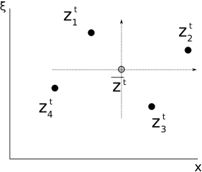
Figure 2. Phase space coordinates relative to the “center of mass”.

We cannot yet integrate by parts since that would require two time derivatives of the phase $\Psi$, but the assumptions on $V$ only allow $\Psi$ to be differentiated once in time. However, we can decompose $\Psi=\Psi_{1}+\Psi_{2}$, where $\Psi_{2}$ has two time derivatives and accounts for the majority of the oscillation of $e^{i\Psi}$; indeed, we define $\Psi_{1}$ and $\Psi_{2}$ via the ODE

$$-L\Psi_{2} =\frac{1}{2}\sum_{j}\sigma_{j}|\overline{\xi^{t}}_{j}|^{2}=\frac{1}{4}\Bigl{(}|\xi_{1}^{t_{q}}-\xi_{2}^{t_{q}}|^{2}-|\xi_{3}^{t_{q}}-\xi_{4}^{t_{q}}|^{2}\Bigr{)}+O(N^{-2+2\delta}),$$

$$-L\Psi_{1} =\sum\sigma_{j}\Bigl{[}V^{\overline{z}}(t,\overline{x^{t}}_{j})+\langle x-x_{j}^{t},\partial_{x}(V^{\overline{z}})(t,\overline{x^{t}}_{j})\rangle\Bigr{]}=O(N^{-2+2\delta});$$

As before we have frozen $t=t_{q}$ in the main term with error at most $O(N^{-2+2\delta})$, and also used the estimates $|\overline{x^{t}}_{j}|\leq\max_{j,k}|x^{t}_{j}-x^{t}_{k}|\lesssim N^{1+\delta}$, $|x-x_{j}^{t}|\lesssim N^{1+\delta}$ on the support of the integrand (49). Note also that the equation $\tfrac{d}{dt}\xi_{j}^{t}=-\partial_{x}V(t,x_{j}^{t})$ implies $L^{2}\Psi_{2}=O(N^{-2})$. Now integrate by parts using the phase $\Psi_{2}$ to obtain

$$\textrm{RH}~{}\eqref{e:kernel_xt_integral} =\int e^{i\Psi_{2}}e^{i\Psi_{1}}\prod_{j}\phi_{j}\,\eta_{N}(t)\,dxdt=i\int e^{i\Psi_{2}}\bigl{\langle}L,\frac{L\Psi_{2}}{|L\Psi_{2}|^{2}}\rangle e^{i\Psi_{1}}\phi_{1}\phi_{2}\overline{\phi_{3}}\overline{\phi_{4}}\,\eta_{N}(t)dxdt$$

$$=i\int e^{i\Psi}\Bigl{[}-\frac{L^{2}\Psi_{2}}{|L\Psi_{2}|^{2}}+\langle\frac{L\Psi_{2}}{|L\Psi_{2}|^{2}},iL\Psi_{1}+L\rangle\Bigr{]}\phi_{1}\phi_{2}\overline{\phi_{3}}\overline{\phi_{4}}\,\eta_{N}(t)dxdt,$$

and the second bound in the lemma follows. ∎

Returning to the proof of Lemma 6.9, we decompose the sum

$$\sum_{(T_{1},T_{2}^{\prime})\in\mathbf{T}_{1}^{\prime}\times\mathbf{T}_{2}^{\prime}}\Bigl{[}\sum_{T_{1}^{\prime}\in\mathbf{T}^{s}_{1}}\sum_{T_{2}\in\mathbf{T}_{2}^{\prime}}+\sum_{0\leq k\lesssim\log N}\sum_{T_{1}^{\prime}\in\mathbf{T}_{1,k}^{\prime}}\sum_{T_{2}\in\mathbf{T}_{2}^{\prime}}\Bigr{]},$$

where $\mathbf{T}^{s}_{1}$ is the set of tubes in $\mathbf{T}_{1}^{\prime}$ whose bicharacteristic $((x_{1}^{\prime})^{t},(\xi_{1}^{\prime})^{t})$ satisfies $(\xi_{1}^{\prime})^{t_{q}}\in\pi^{s}(\xi_{1}^{t_{q}},(\xi_{2}^{\prime})^{t_{q}})$, and we abbreviate

$$\mathbf{T}_{1,k}^{\prime}:=\mathbf{T}_{1}^{\nsim B}(q,\lambda_{1},\mu_{1},\mu_{2},\xi_{1}^{t_{q}},(\xi_{2}^{\prime})^{t_{q}},k)$$

The contribution from the “space nonresonance” terms $\mathbf{T}^{s}_{1}$ is $O(N^{-100d})$.

Now consider the $k$th sum. Lemma 6.10 implies that

$$|\langle\phi_{T_{1}}\phi_{T_{2}},\,\phi_{T_{1}^{\prime}}\phi_{T_{2}^{\prime}}\rangle|\lesssim N^{C\delta}N^{-(d-1)}2^{-k}.$$

For each $T_{1}^{\prime}\in\mathbf{T}_{1}^{\nsim B}(q,\lambda_{1},\mu_{1},\mu_{2},\xi_{1}^{t_{q}},(\xi_{2}^{\prime})^{t_{q}},k)$, the possible tubes $T_{2}$ correspond to the bicharacteristics $(x_{2}^{t},x_{2}^{t})$ such that

$$|x_{2}^{t_{q}}-x_{q}|\leq N^{1+\delta},\quad\xi_{1}^{t_{q}}+\xi_{2}^{t_{q}}-(\xi_{1}^{\prime})^{t_{q}}-(\xi_{2}^{\prime})^{t_{q}}=O(N^{-1+C\delta}).$$

The preimage of this set under the time $t_{q}$ Hamiltonian flow map is a $(N^{1+C\delta})^{d}\times(N^{-1+C\delta})^{-d}$ box, so there are $O(N^{C\delta})$ choices of tubes $T_{2}$. Therefore, the $k$th sum is at most

$$N^{C\delta}N^{-(d-1)}2^{-k}\nu_{k}\#\mathbf{T}_{1}^{\prime}\#\mathbf{T}_{2}^{\prime},$$

whereupon the sum over $k$ is replaced by the supremum at the cost of a $\log N$ factor. ∎

It remains to show that

(50) $$\sum_{q\in\mathbf{q}(\mu_{1},\mu_{2}):q\subset 2B}2^{-k}\nu_{k}(q,\lambda_{1},\mu_{1},\mu_{2})\#(\mathbf{T}_{1}^{\nsim B}(q)\cap\mathbf{T}_{1}[\lambda_{1},\mu_{1},\mu_{2}])\#\mathbf{T}_{2}(q)\lessapprox N^{C\delta}\#\mathbf{T}_{1}\#\mathbf{T}_{2}.$$

6.9. Tube combinatorics

This section begins exactly as in [Tao03, Section 8]. We define the relation $\sim$ between tubes and radius $N^{2(1-\delta)}$ balls. For a tube $T\in\mathbf{T}_{1}[\lambda_{1},\mu_{1},\mu_{2}]$, let $B(T,\lambda_{1},\mu_{1},\mu_{2})$ be a ball $B\in\mathcal{B}$ that maximizes

$$\#\{q\in\mathbf{q}(\mu_{1},\mu_{2}):T\cap N^{\delta}q\neq\phi;\ q\cap B\neq\phi\}.$$

As $T$ intersects roughly $\lambda_{1}$ (neighborhoods of) balls $q\in\mathbf{q}(\mu_{1},\mu_{2})$ in total and there are $O(N^{2\delta})$ many balls in $\mathcal{B}$, $B(T,\lambda_{1},\mu_{1},\mu_{2})$ must intersect at least $N^{-2\delta}\lambda_{1}$ of those balls.

Declare $T\sim_{\lambda_{1},\mu_{1},\mu_{2}}B^{\prime}$ if $T\in\mathbf{T}_{1}[\lambda_{1},\mu_{1},\mu_{2}]$ and $B^{\prime}\subset 10B(T,\lambda_{1},\mu_{1},\mu_{2})$. Finally, for $T\in\mathbf{T}_{1}$ set $T\sim B$ if $T\sim_{\lambda_{1},\mu_{1},\mu_{2}}B$ for some $\lambda_{1},\mu_{1},\mu_{2}$. Evidently $T\sim B$ for at most $(\log N)^{3}\lessapprox 1$ many balls. The relation between tubes in $\mathbf{T}_{2}$ and balls in $\mathcal{B}$ is defined similarly.

Now we begin the proof of (50). On one hand,

$$\sum_{q\in\mathbf{q}(\mu_{1},\mu_{2})}\#(\mathbf{T}_{1}[\lambda_{1},\mu_{1},\mu_{2}]\cap\mathbf{T}_{1}(q)) =\sum_{q\in\mathbf{q}(\mu_{1},\mu_{2})}\sum_{T_{1}\in\mathbf{T}_{1}[\lambda_{1},\mu_{1},\mu_{2}]\cap\mathbf{T}_{1}(q)}1_{T_{1}\cap N^{\delta}q\neq 0}$$

$$=\sum_{T\in\mathbf{T}_{1}[\lambda_{1},\mu_{1},\mu_{2}]}\sum_{q\in\mathbf{q}(\mu_{1},\mu_{2})}1_{T_{1}\cap N^{\delta}q\neq\phi}$$

$$\lesssim\sum_{T\in\mathbf{T}_{1}}\lambda_{1}$$

$$=\lambda_{1}\#\mathbf{T}_{1}.$$

On the other hand, by definition $\#\mathbf{T}_{2}(q)\lesssim\mu_{2}$. The claim (50) would therefore follow if we could show that

(51) $$\nu_{k}(q_{0},\lambda_{1},\mu_{1},\mu_{2})\lessapprox 2^{k}N^{C\delta}\frac{\#\mathbf{T}_{2}}{\lambda_{1}\mu_{2}}$$

for all $q_{0}\in\mathbf{q}(\mu_{1},\mu_{2})$ such that $q_{0}\subset 2B$.

Fix $\xi_{1}\in S_{1}$, $\xi_{2}^{\prime}\in S_{2}$, and a ball $q_{0}=q_{0}(t_{q},x_{q})$. Recalling the definition (48) of $\nu_{k}$, we need to show that

$$\#\mathbf{T}^{\nsim B}_{1}(q_{0},\lambda_{1},\mu_{1},\mu_{2},\xi_{1}^{t_{q}},(\xi_{2}^{\prime})^{t_{q}},k)\lessapprox 2^{k}N^{C\delta}\frac{\#\mathbf{T}_{2}}{\lambda_{1}\mu_{2}}.$$

For brevity write $\mathbf{T}_{1}^{\prime}:=\mathbf{T}^{\nsim B}_{1,k}(q_{0},\lambda_{1},\mu_{1},\mu_{2},\xi_{1}^{t_{q}},(\xi_{2}^{\prime})^{t_{q}},k)$.

Fix $T_{1}\in\mathbf{T}_{1}^{\prime}$. Since $T_{1}\nsim B$, the ball $2B(T_{1},\lambda_{1},\mu_{1},\mu_{2})$ has distance $\gtrsim N^{2(1-\delta)}$ from $q_{0}$. Thus

$$\#\{q\in\mathbf{q}(\mu_{1},\mu_{2}):T_{1}\cap N^{\delta}q\neq\phi,\ \operatorname{dist}(q,q_{0})\gtrapprox N^{2(1-\delta)}\}\gtrapprox N^{-2\delta}\lambda_{1}.$$

As each $q\in\mathbf{q}(\mu_{1},\mu_{2})$ intersects approximately $\mu_{2}$ ($N^{\delta}$-neighborhoods of) tubes in $\mathbf{T}_{2}$,

$$\#\{(q,T_{2})\in\mathbf{q}(\mu_{1},\mu_{2})\times\mathbf{T}_{2}:T_{1}\cap N^{\delta}q\neq\phi,\ T_{2}\cap N^{\delta}q\neq\phi,\ \operatorname{dist}(q,q_{0})\gtrapprox N^{2(1-\delta)}\}\gtrapprox N^{-2\delta}\lambda_{1}\mu_{2}.$$

Therefore

$$\#\{(q,T_{1},T_{2})\in\mathbf{q}\times\mathbf{T}_{1}^{\prime}\times\mathbf{T}_{2}:T_{1}\cap N^{\delta}q\neq\phi,\ T_{2}\cap N^{\delta}q\neq\phi,\ \operatorname{dist}(q,q_{0})\gtrapprox N^{-2\delta}N^{2}\}$$

$$\gtrapprox N^{-2\delta}\lambda_{1}\mu_{2}\#\mathbf{T}_{1}^{\prime}$$

On the other hand, the cardinality can be bounded above by the following analogue of Tao’s Lemma 8.1:

Lemma 6.11.

For each $T_{2}\in\mathbf{T}_{2}$,

$$\#\{(q,T_{1})\in\mathbf{q}\times\mathbf{T}_{1}^{\prime}:T_{1}\cap N^{\delta}q,\ T_{2}\cap N^{\delta}q\neq\phi,\ \operatorname{dist}(q,q_{0})\gtrapprox N^{-2\delta}N^{2}\}\lessapprox 2^{k}N^{C\delta}.$$

Proof.

We estimate in two steps.

• For any tubes $T_{1}\in\mathbf{T}_{1}^{\prime}$ and $T_{2}\in\mathbf{T}_{2}$, the intersection $N^{\delta}T_{1}\cap N^{\delta}T_{2}$ is contained in a ball of radius $N^{C\delta}$.

• The number of tubes $T_{1}\in\mathbf{T}_{1}^{\prime}$ such that $T_{1}$ intersects $N^{\delta}T_{2}$ at distance $\gtrapprox N^{-2\delta}N^{2}$ from $q_{0}$ bounded above by $2^{k}N^{C\delta}$.

The first is evident from transversality. Hence we turn to the second claim.

In Tao’s situation, the tubes in $\mathbf{T}_{1}^{\prime}$ are all constrained to a $O(N^{-1+C\delta})$ neighborhood of a spacetime hyperplane transverse to the tube $T_{2}$ (basically because of Lemma 6.8), and there are $O(N^{C\delta})$ many such tubes that intersect $T_{2}$ at distance $\gtrapprox N^{-2\delta}N^{2}$ from $q_{0}$. The extra $2^{k}$ factor results from the fact that we allow the tubes to deviate from that hyperplane by distance $2^{k}N^{-1+C\delta}$. Also, since our tubes are curved it is more convenient to work with their associated bicharacteristics instead of using Euclidean geometry in spacetime.

Fix a tube $T_{2}\in\mathbf{T}_{2}$ with ray $t\mapsto(x_{2}^{t},\xi_{2}^{t})$. Then, the tubes $T_{1}\in\mathbf{T}_{1}^{\prime}$ such that $N^{\delta}T_{1}\cap N^{\delta}T_{2}$ are characterized by the property that

$$|x(T_{1})^{t}-x_{2}^{t}|\lesssim N^{1+\delta}\text{ for some }|t-t_{q}|\gtrapprox N^{-2\delta}N^{2}.$$

We need to count the tubes in $\mathbf{T}_{1}^{\prime}$ with this property. The bicharacteristics for such tubes emanate from the region

$$\Sigma:= \{(x,\xi):\operatorname{dist}(\xi,S_{1})\leq N^{-1+C\delta},\ \xi^{t_{q}}\in\pi^{t}_{k},$$

$$|x^{t_{q}}-x_{q}|\leq N^{1+\delta},\ |x^{t}-x_{2}^{t}|\leq N^{1+\delta}\text{ for some }|t-t_{q}|\gtrsim N^{-2\delta}N^{2}\},$$

hence it suffices to bound the cardinality of the intersection $(N\mathbf{Z}^{d}\times N^{-1}\mathbf{Z}^{d})\cap\Sigma$.

Denote by $\Sigma^{t}$ the image of $\Sigma$ under the time $t$ Hamiltonian flow map $(x,\xi)\mapsto(x^{t},\xi^{t})$. Recall from (38) that $S_{j}^{t}$ denotes the image of the initial frequency set $S_{j}$ for initial positions $x$ with $|x|\lesssim N^{2}$; we saw earlier in (40) that $S_{j}^{t}$ is a small perturbation of $S_{j}$.

Fix a basepoint $x_{0}$ with $|x_{0}-x_{q}|\leq N^{1+\delta}$. By Lemma 2.1 and the Hadamard global inverse function theorem, when $t\neq t_{q}$ we can parametrize the graph of the flow map $(x^{t_{q}},\xi^{t_{q}})\mapsto(x^{t},\xi^{t})$ by the variables

$$(x^{t_{q}},x^{t})\mapsto\bigl{(}(x^{t_{q}},\xi^{t_{q}}(x^{t},x^{t_{q}}))\mapsto(x^{t},\xi^{t}(x^{t_{q}},x^{t}))\bigr{)}.$$

Let $\xi(t,x):=\xi^{t_{q}}(x_{0},x)\in T^{*}_{x_{0}}\mathbf{R}^{d}$ be the initial momentum $\xi(t,x)\in T^{*}_{x_{0}}\mathbf{R}^{d}$ such that the bicharacteristic with $x^{t_{q}}=x_{0}$ and $\xi^{t_{q}}=\xi(t,x)$ satisfies $x^{t}=x$.

Lemma 6.12.

Suppose at least one $T_{1}\in\mathbf{T}_{1}^{\prime}$ intersects $N^{\delta}T_{2}$. For $|t-t_{q}|\gtrapprox N^{-2\delta}N^{2}$, the curve $t\mapsto\zeta_{x_{0}}(t):=\xi(t,x_{2}^{t})\in T^{*}_{x_{0}}\mathbf{R}^{d}$ is transverse to the hyperplane containing $\pi(\xi_{1},\xi_{2}^{\prime})$ for all $\xi_{1}\in S_{1}^{t_{q}}$ and $\xi_{2}^{\prime}\in S_{2}^{t_{q}}$ (see Figure 3). More precisely there exists $C(\eta)>0$ such that

$$\angle(\dot{\zeta}_{x_{0}}(t),\pi(\xi_{1},\xi_{2}^{\prime}))>C(\eta)\text{ for all }\xi_{1}\in S_{1}^{t_{q}},\ \xi_{2}^{\prime}\in S_{2}^{t_{q}},$$

where the angle $\angle(v,W)$ between a vector $v$ and a subspace $W$ is defined in the usual manner. Moreover, for each $t$ the image of a $N^{1+\delta}$ neighborhood of $x_{2}^{t}$ under the map $x\mapsto\xi(t,x)$ belongs to a $N^{-1+C\delta}$ neighborhood of $\zeta_{x_{0}}(t)$.

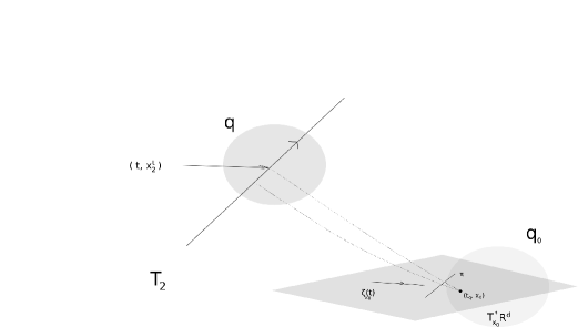
Figure 3. $\zeta_{x_{0}}(t)\in T^{*}_{x_{0}}\mathbf{R}^{d}$ is the set of tangent (covectors) for rays passing through $(t_{q},x_{0})$ that intersect the ray $(t,x_{2}^{t})$ for the tube $T_{2}$ at times $|t-t_{q}|\gtrapprox N^{2-2\delta}$.

Proof.

By a slight abuse of notation we write $\bigl{(}x^{t}(y,\zeta),\xi^{t}(y,\zeta)\bigr{)}$ for the bicharacteristic passing through $(y,\zeta)$ at time $t=t_{q}$ instead of $t=0$. Both claims are consequences of Lemma 2.1, which yields

$$x_{2}^{t} =x^{t}(x_{0},\zeta_{x_{0}}(t)),\quad\xi^{t_{q}}(x_{0},\zeta_{x_{0}}(t))=\zeta_{x_{0}}(t),$$

$$\xi_{2}^{t} =\frac{d}{dt}x_{2}^{t}=\xi^{t}\bigl{(}x_{0},\zeta_{x_{0}}(t)\bigr{)}+\frac{\partial x^{t}}{\partial\zeta_{x_{0}}}\dot{\zeta}_{x_{0}}(t)$$

$$=\xi^{t}(x_{0},\zeta_{x_{0}}(t))+(t-t_{q})\bigl{(}I+O(\eta)\bigr{)}\dot{\zeta}_{x_{0}}(t),$$

therefore

(52) $$\dot{\zeta}_{x_{0}}(t)=(t-t_{q})^{-1}\bigl{(}I+O(\eta)\bigr{)}\bigl{(}\xi_{2}^{t}-\xi^{t}(x_{0},\zeta_{x_{0}}(t))\bigr{)}.$$

We claim that for any $C>1$,

(53) $$\operatorname{dist}(\zeta_{x_{0}}(t_{q}),S_{1}^{t_{q}})\lesssim_{C}N^{-1+C\delta}.$$

Otherwise, as $|t-t_{q}|\gtrapprox N^{2(1-\delta)}$, for any ray $(x_{1}^{t},\xi_{1}^{t})$ with $\xi_{1}\in S_{1}$ and $|x_{1}^{t_{q}}-x_{q}|\leq N^{1+\delta}$, the estimates (21) would imply that

$$|x_{1}^{t}-x_{2}^{t}| \gtrsim|t-t_{q}||\xi_{1}^{t_{q}}-\zeta_{x_{0}}(t)|-|x_{1}^{t_{q}}-x_{0}|$$

$$\gtrsim N^{-1+C\delta}-N^{1+\delta}\gtrsim N^{1+C\delta},$$

so we get the contradiction that every $T_{1}\in\mathbf{T}_{1}^{\prime}$ misses $T_{2}$ by at least $N^{C\delta}$.

By the near-constancy (40) of the frequency variable and the definition (31) of $S_{j}$, the covector $\xi_{2}^{t}-\xi^{t}(x_{0},\zeta_{x_{0}}(t))$ belongs a small perturbation (say, of magnitude at most $\tfrac{c}{50}$) of the difference set $S_{2}-S_{1}=-2ce_{1}+B(0,\tfrac{c}{50})$, hence by Lemma 6.8 is transverse to the hyperplane containing $\pi(\xi_{1},\xi_{2}^{\prime})$. The first claim now follows from (52).

The argument just given also implies the second statement: a ray with $x^{t_{q}}=x_{0}$ and $|x_{2}^{t}-x^{t}|\leq N^{1+\delta}$ must satisfy $|\xi^{t_{q}}-\zeta_{x_{0}}(t)|\lesssim N^{-1+C\delta}$. ∎

By the second part of the lemma, the fiber of $\Sigma^{t_{q}}$ in $T_{x_{0}}^{*}\mathbf{R}^{d}$ is contained in a “frequency tube”

$$\Theta(x_{0}):=\bigcup_{|t-t_{q}|\gtrapprox N^{2(1-\delta)}}B(\zeta_{x_{0}}(t),N^{-1+C\delta}).$$

As the basepoint $x_{0}$ varies in $N^{1+\delta}$ neighborhood of $x_{q}$, the estimate (21) implies that the curve $\zeta_{x_{0}}(t)$ shifts by at most $O(N^{-1+3\delta})$. Hence the tubes $\Theta(x_{0})$ are all contained in a dilate of $\Theta(x_{q})$, which we denote by

$$\widetilde{\Theta}(x_{q}):=\bigcup_{t}B(\zeta_{x_{q}}(t),N^{-1+C\delta})$$

with a larger $C$.

Therefore, $\Sigma^{t_{q}}$ is contained in the region

$$\tilde{\Sigma}^{t_{q}}:=\bigl{\{}(x,\xi):|x-x_{q}|\leq N^{1+\delta},\ \xi\in\pi^{t}_{k}\cap\widetilde{\Theta}(x_{q})\subset\{\xi\in\widetilde{\Theta}(x_{q}):\operatorname{dist}(\xi,\pi)\lesssim 2^{k}N^{-1+C\delta}\}\bigr{\}},$$

where for the last containment we recall the estimate (47). The region $\tilde{\Sigma}^{t_{q}}$ is sketched in Figure 4.

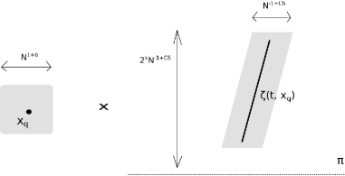
Figure 4. The phase space region $\Sigma^{t_{q}}$.

Using the previous lemma for the central curve $\zeta_{x_{q}}$, the frequency projection $(x,\xi)\mapsto\xi)$ of $\tilde{\Sigma}^{t_{q}}$ can be covered by approximately $2^{k}$ finitely overlapping cubes $\bigcup_{1\leq j\lesssim 2^{k}}Q_{j}$ of width $N^{-1+C\delta}$. By (21), the preimage of each box

$$B(x_{q},N^{1+\delta})\times Q_{j}$$

under the flow map $(x,\xi)\mapsto(x^{t_{q}},\xi^{t_{q}})$ is contained in a $(CN^{1+C\delta})^{d}\times(CN^{-1+C\delta})^{d}$ box. The union of these preimages cover $\Sigma$ and contain at most $O(2^{k}N^{C\delta})$ points in $N\mathbf{Z}^{d}\times N^{-1}\mathbf{Z}^{d}$. ∎

7. Remarks on magnetic potentials

We sketch the modifications needed to prove Theorem 1.6. The symbol for $H(t)$ is

$$a=\frac{1}{2}|\xi|^{2}+\langle A,\xi\rangle+V(t,x),$$

where $A=A_{j}(t,x)dx^{j}$ and $A_{j}$ are linear functions in the space variables with bounded time-dependent coefficients.

• Easy computation shows that the symbol map $a\mapsto a^{z_{0}}$ in Lemma 1.1 is

  $$a^{z_{0}}=\frac{1}{2}|\xi|^{2}+\langle A_{(1)}^{z_{0}}(t,x),\xi\rangle+\langle A_{(2)}^{z_{0}}(t,x),\xi_{0}^{t}\rangle+V_{(2)}^{z_{0}}(t,x),$$

  where $A_{(1)}^{z_{0}}(t,x)=A(t,x_{0}^{t}+x)-A(t,x_{0}^{t})$ and $A_{(2)}^{z_{0}}(t,x)=A(t,x_{0}^{t}+x)-\langle x,\partial_{x}A(t,x_{0}^{t})\rangle-A(x_{0}^{t})$, and similarly for $V$. Thus when $A$ is linear, the first order component of the symbol is exactly “Galilei-invariant”, preserved by the transformation $a\mapsto a^{z_{0}}$ in Lemma 1.1.

• After rescaling, the inequality (15) takes the form

  $$\|U_{N}fU_{N}g\|_{L^{\frac{d+3}{d+1}}([-\tau_{0}N^{2},\tau_{0}N^{2}]\times\mathbf{R}^{d})}\lesssim_{\varepsilon}N^{\varepsilon}\|f\|_{L^{2}}\|g\|_{L^{2}},$$

  where $U_{N}(t)$ be the propagator for the rescaled symbol

  $$a_{N} :=N^{-2}a(N^{-2}t,N^{-1}x,N\xi)=\frac{1}{2}|\xi|^{2}+N^{-2}\langle A(x),\xi\rangle+N^{-2}V(N^{-2}t,N^{-1}x).$$

• Exploiting Galilei-invariance, we may reduce to a spatially localized estimate as in Proposition 6.4. Note that in the region of phase space corresponding to that estimate $\{(x,\xi):|x|\leq N^{2},\quad|\xi|\lesssim 1\}$, and over a $O(N^{2})$ time interval, both potential terms have strength $O(1)$ when integrated over the time interval $|t|\lesssim N^{2}$. However the magnetic term dominates near $x=0$.

• Then, the rest of the previous proof can be mimicked with essentially no change except for Lemma 6.10. There, one argues essentially as before except the vector field $L$ for integrating by parts should be replaced by

  $$L:=\partial_{t}+\langle\overline{a_{\xi}(z_{j}^{t})},\partial_{x}\rangle,$$

  where $z_{j}^{t}=(x_{j}^{t},\xi_{j}^{t})$ and $\overline{a_{\xi}(z_{j}^{t})}=\tfrac{1}{4}\sum_{k}a_{\xi}(z_{k}^{t})$. Then one finds that

  $$-L\Psi=\frac{1}{2}\sum_{j}\sigma_{j}|\overline{\xi^{t}}_{j}|^{2}+\sum_{j}\sigma_{j}\langle A(\overline{x^{t}}_{j}),\xi_{j}^{t}\rangle+\sum_{j}\sigma_{j}\bigl{[}V^{\overline{z}}(t,\overline{x^{t}}_{j})+\langle x-x_{j}^{t},\partial_{x}(V^{\overline{z}})(t,\overline{x^{t}}_{j})\rangle\bigr{]},$$

  and decomposes as before $\Psi=\Psi_{1}+\Psi_{2}$, where

  $$-L\Psi_{1} =\frac{1}{2}\sum_{j}\sigma_{j}|\overline{\xi^{t}}_{j}|^{2}=|\xi_{1}^{t_{q}}-\xi_{2}^{t_{q}}|^{2}-|\xi_{3}^{t_{q}}-\xi_{4}^{t_{q}}|^{2}+O(N^{-1+\delta})$$

  $$-L\Psi_{2} =\sum_{j}\sigma_{j}\langle A(\overline{x^{t}}_{j}),\xi_{j}^{t}\rangle+\sum_{j}\sigma_{j}\bigl{[}V^{\overline{z}}(t,\overline{x^{t}}_{j})+\langle x-x_{j}^{t},\partial_{x}(V^{\overline{z}})(t,\overline{x^{t}}_{j})\rangle\bigr{]}$$

  $$=O(N^{-1+\delta}).$$

  As in the proof of Lemma 6.10 the error terms are computed from the estimates (21), $|t-t_{q}|\lesssim N^{1+\delta}$, and $|\overline{x^{t}}_{j}|\lesssim N^{1+\delta}$. The errors are larger than before due to the magnetic term $a_{x\xi}=O(N^{-2})$ but are still acceptable.

References

- [BTT13] N. Burq, L. Thomann, and N. Tzvetkov, Long time dynamics for the one dimensional non linear Schrödinger equation, Ann. Inst. Fourier (Grenoble) 63 (2013), no. 6, 2137–2198. MR 3237443
- [BV07] P. Bégout and A. Vargas, Mass concentration phenomena for the -critical nonlinear Schrödinger equation, Trans. Amer. Math. Soc. 359 (2007), no. 11, 5257–5282. MR 2327030 (2008g:35190)
- [Car11] R. Carles, Nonlinear schrödinger equation with time-dependent potential, Commun. Math Sci. 9 (2011), no. 4, 937–964.
- [CK07] R. Carles and S. Keraani, On the role of quadratic oscillations in nonlinear Schrödinger equations. II. The -critical case, Trans. Amer. Math. Soc. 359 (2007), no. 1, 33–62 (electronic). MR 2247881 (2008a:35260)
- [Dod12] B. Dodson, Global well-posedness and scattering for the defocusing, -critical nonlinear Schrödinger equation when , J. Amer. Math. Soc. 25 (2012), no. 2, 429–463. MR 2869023
- [Dod15] by same author, Global well-posedness and scattering for the mass critical nonlinear Schrödinger equation with mass below the mass of the ground state, Adv. Math. 285 (2015), 1589–1618. MR 3406535
- [Dod16a] by same author, Global well-posedness and scattering for the defocusing, critical, nonlinear Schrödinger equation when , Amer. J. Math. 138 (2016), no. 2, 531–569. MR 3483476
- [Dod16b] by same author, Global well-posedness and scattering for the defocusing, -critical, nonlinear Schrödinger equation when , Duke Math. J. 165 (2016), no. 18, 3435–3516. MR 3577369
- [Fuj79] D. Fujiwara, A construction of the fundamental solution for the Schrödinger equation, J. Analyse Math. 35 (1979), 41–96. MR 555300 (81i:35145)
- [GV95] J. Ginibre and G. Velo, Generalized Strichartz inequalities for the wave equation, J. Funct. Anal. 133 (1995), no. 1, 50–68. MR 1351643 (97a:46047)
- [IPS12] A. D. Ionescu, B. Pausader, and G. Staffilani, On the global well-posedness of energy-critical Schrödinger equations in curved spaces, Anal. PDE 5 (2012), no. 4, 705–746. MR 3006640
- [Jao16] C. Jao, The energy-critical quantum harmonic oscillator, Comm. Partial Differential Equations (2016), no. 1, 79–133.
- [JKV] C. Jao, R. Killip, and M. Visan, Mass-critical inverse Strichartz theorems for 1d Schrödinger operators, To appear in Revista Matemática Iberoamericana.
- [KT98] M. Keel and T. Tao, Endpoint Strichartz estimates, Amer. J. Math. 120 (1998), no. 5, 955–980. MR 1646048 (2000d:35018)
- [KT05] H. Koch and D. Tataru, Dispersive estimates for principally normal pseudodifferential operators, Comm. Pure Appl. Math. 58 (2005), no. 2, 217–284. MR 2094851
- [KTV09] R. Killip, T. Tao, and M. Visan, The cubic nonlinear Schrödinger equation in two dimensions with radial data, J. Eur. Math. Soc. (JEMS) 11 (2009), no. 6, 1203–1258. MR 2557134 (2010m:35487)
- [KV13] R. Killip and M. Vişan, Nonlinear Schrödinger equations at critical regularity, Evolution equations, Clay Math. Proc., vol. 17, Amer. Math. Soc., Providence, RI, 2013, pp. 325–437. MR 3098643
- [KVZ] R. Killip, M. Visan, and X. Zhang, Quintic NLS in the exterior of a strictly convex obstacle, To appear in Amer. J. Math.
- [KVZ08] by same author, The mass-critical nonlinear Schrödinger equation with radial data in dimensions three and higher, Anal. PDE 1 (2008), no. 2, 229–266. MR 2472890
- [MV98] F. Merle and L. Vega, Compactness at blow-up time for solutions of the critical nonlinear Schrödinger equation in 2D, Internat. Math. Res. Notices (1998), no. 8, 399–425. MR 1628235 (99d:35156)
- [MVV99] A. Moyua, A. Vargas, and L. Vega, Restriction theorems and maximal operators related to oscillatory integrals in , Duke Math. J. 96 (1999), no. 3, 547–574. MR 1671214
- [PRT14] A. Poiret, D. Robert, and L. Thomann, Probabilistic global well-posedness for the supercritical nonlinear harmonic oscillator, Anal. PDE 7 (2014), no. 4, 997–1026. MR 3254351
- [RV06] K. M. Rogers and A. Vargas, A refinement of the Strichartz inequality on the saddle and applications, J. Funct. Anal. 241 (2006), no. 1, 212–231. MR 2264250
- [Str77] R. S. Strichartz, Restrictions of Fourier transforms to quadratic surfaces and decay of solutions of wave equations, Duke Math. J. 44 (1977), no. 3, 705–714. MR 0512086
- [Tao03] T. Tao, A sharp bilinear restrictions estimate for paraboloids, Geom. Funct. Anal. 13 (2003), no. 6, 1359–1384. MR 2033842 (2004m:47111)
- [TVZ07] T. Tao, M. Visan, and X. Zhang, Global well-posedness and scattering for the defocusing mass-critical nonlinear Schrödinger equation for radial data in high dimensions, Duke Math. J. 140 (2007), no. 1, 165–202. MR 2355070 (2010a:35249)
- [Var05] A. Vargas, Restriction theorems for a surface with negative curvature, Math. Z. 249 (2005), no. 1, 97–111. MR 2106972
- [Wol01] T. Wolff, A sharp bilinear cone restriction estimate, Ann. of Math. (2) 153 (2001), no. 3, 661–698. MR 1836285 (2002j:42019)
- [Yaj91] K. Yajima, Schrödinger evolution equations with magnetic fields, J. Analyse Math. 56 (1991), 29–76. MR 1243098
- [Zha00] J. Zhang, Stability of attractive Bose-Einstein condensates, J. Statist. Phys. 101 (2000), no. 3-4, 731–746. MR 1804895 (2002b:82039)
- [Zha05] by same author, Sharp threshold for blowup and global existence in nonlinear Schrödinger equations under a harmonic potential, Comm. Partial Differential Equations 30 (2005), no. 10-12, 1429–1443. MR 2182299