A numerical study of a variable-density
low-speed turbulent mixing layer

Abstract

Direct numerical simulations of a temporally-developing, low-speed, variable-density, turbulent, plane mixing layer are performed. The Navier-Stokes equations in the low-Mach number approximation are solved using a novel algorithm based on an extended version of the velocity-vorticity formulation used by Kim et al. (1987) for incompressible flows. Four cases with density ratios $s=1,2,4$ and 8 are considered. The simulations are run with a Prandtl number of 0.7 and achieve a $Re_{\lambda}$ up to 150 during the self-similar evolution of the mixing layer. It is found that the growth rate of the mixing layer decreases with increasing density ratio, in agreement with theoretical models of this phenomenon. Comparison with high-speed data shows that the reduction of the growth rates with increasing the density ratio has a weak dependence with the Mach number. In addition, the shifting of the mixing layer to the low-density stream has been characterized by analyzing one point statistics within the self-similar interval. This shifting has been quantified, and related to the growth rate of the mixing layer under the assumption that the shape of the mean velocity and density profiles do not change with the density ratio. This leads to a predictive model for the reduction of the growth rate of the momentum thickness, which agrees reasonably well with the available data. Finally, the effect of the density ratio on the turbulent structure has been analyzed using flow visualizations and spectra. It is found that with increasing density ratio the longest scales in the high density side are gradually inhibited. A gradual reduction of the energy in small scales with increasing density ratio is also observed.

1 Introduction

Variable density effects in turbulent flows are often encountered in the natural environment and in many engineering applications (Chassaing et al., 2002; Turner, 1979). In the oceans, density variations are due to temperature and salinity variations (Thorpe, 2005), while in the atmosphere they are due to both temperature and moisture changes (Wyngaard, 2010). In both situations, the buoyancy effects are mainly due to gravity. In absence of gravity, density effects may still be important due to pressure and/or temperature fluctuations. For example in aeronautical applications, density variations due to high speed in gas flows are very relevant (Lele, 1994; Gatski and Bonnet, 2013). In that case, the main effect is due to velocity induced pressure variations. In other applications, density variations due to dilatation effects are important even at low speeds. This is for example the case in combustion applications (Williams, 1985; Peters, 2000), where the heat release by chemical reaction leads to the thermal expansion of the fluid. An additional kind of density effect is associated with the mixing of two non-reactive fluids of different density or to the mixing of different temperature bodies of the same fluid (Chassaing et al., 2002; Dimotakis, 2005). In this work we are concerned with the latter since we study a variable-density low-speed temporal turbulent mixing layer in the absence of gravity.

As reviewed by Dimotakis (1986), in spatially-developing turbulent shear layers the density ratio influences the spreading rate of the layer, the entrainment rate and the convective velocity of the large-scale eddies. The influence on the spreading rate was already observed in early experiments (Brown and Roshko, 1974). However, the effect of increasing the Mach number, $M$, was found to be more drastic and that led to a main focus on compressibility effects in subsequent works (Bogdanoff, 1983; Papamoschou and Roshko, 1988; Clemens and Mungal, 1992; Hall et al., 1993; Vreman et al., 1996; Mahle et al., 2007; O’Brien et al., 2014; Jahanbakhshi and Madnia, 2016). A notable exception is the work of Pantano and Sarkar (2002) who studied both compressibility effects and density ratio effects in direct numerical simulations of turbulent compressible temporal mixing layers. They found that, with increasing density ratio, the shear layer growth rate decreases substantially and that the dividing streamline is shifted towards the low-density stream. The variation of the density ratio by Pantano and Sarkar (2002) was performed at high speed, with a convective Mach number $M_{c}=0.7$, so that density variations due to both pressure effects and temperature effects were likely to affect the flow. In this work we try to separate these two effects by considering a variable-density layer at low speed in the limit $M_{c}\rightarrow 0$, using the low Mach number approximation (McMurtry et al., 1986; Cook and Riley, 1996; Nicoud, 2000).

The current understanding of the effect of the density ratio on the structure of the turbulent mixing layer is still unsatisfactory. Part of the problem is that it is difficult to perform experiments at low speeds with a large density ratio. Numerical studies are also scarce and most of them deal with the initial stages of transition to turbulence, and not with the turbulent regime itself. Most numerical studies consider variable density effects in the limit of incompressible flow, i.e. the velocity field is solenoidal, the density is given by an advection equation and the energy equation is therefore decoupled from the momentum equation. For instance, Knio and Ghoniem (1992) reported calculations of a variable-density, incompressible, temporal mixing layer. They performed visualizations of the vorticity and scalar fields and of the motion of material surfaces, focusing on the manifestation of three dimensional instabilities. They found an asymmetric entrainment pattern favouring the low-density stream. Also in the incompressible regime, Soteriou and Ghoniem (1995) performed two-dimensional simulations of spatially-developing variable-density mixing layers. They found that the speed of the unstable waves is biased toward that of the high-density stream and also that the entrainment of the high-density stream is inhibited relative to the low-density stream. The instability characteristics of variable-density incompressible mixing layers have been studied by Reinaud et al. (2000) and Fontane and Joly (2008). On the modelling side, Ramshaw (2000) developed a simple model for predicting the thickness of a variable-density mixing layer. Ashurst and Kerstein (2005) included variable-density effects in a one-dimensional turbulence approach. Using this approach they studied both temporally-developing and spatially-developing mixing layers, and despite the limitations of the approach, their results provide information concerning the expected behaviour of the mixing layers at high density ratios. In addition, there are also not so many studies in the literature using Large Eddy Simulation (LES) in variable density turbulent flows. Some examples are Wang et al. (2008), who analyzed spatially developing axisymmetric jets, and McMullan et al. (2011), who considered a spatially developing mixing.

In this work we address the following issues. How is the growth rate of the turbulent mixing layers affected by the free-stream density ratio? What is the turbulent structure of variable-density mixing layers? What are the differences of the low speed case, $M\rightarrow 0$, with respect to the high speed case, $M_{c}=0.7$ (Pantano and Sarkar, 2002)? The manuscript is organized as follows. In §2 the computational setup is described including the details of a novel algorithm developed to solve the low Mach number approximation of the Navier-Stokes equations. This is followed by a description of the simulation parameters in §3. Results are presented in §4. First, we analyze the self-similar evolution of the mixing layers. Secondly, we characterize their growth rate and compare to a model proposed in the literature. Third, we analyze the mean density and Favre averaged velocity, and propose a semi-empirical model for the observed shifting. After this, we complete the characterization of the vertical profiles with mean temperature. This is followed in §4.4 by the analysis of the higher order statistics. Section 4 finalizes with the analysis of the flow structures, using flow visualizations and premultiplied spectra of temperature and velocity. Conclusions are provided in §5.

2 Computational setup

The flow under consideration is a three-dimensional, temporally-evolving mixing layer developing between two streams of different density, $\rho_{t}$ (upper stream) and $\rho_{b}$ (lower stream). The flow is assumed to be homogeneous in the horizontal directions, $x$ and $z$, while it is inhomogeneous in the vertical direction, $y$. The lower stream flows at a velocity $\Delta U/2$ in the positive $x$ direction, while the upper stream flows at a velocity $\Delta U/2$ in the oposite direction, so that the velocity difference between both streams is $\Delta U$. For the present work, $\rho_{b}>\rho_{t}$, although since we do not consider gravity effects, the case with $\rho_{b}<\rho_{t}$ can be obtained by changing the direction of the $y$-axis.

As explained in the introduction, for the present study we consider that temperature and density fluctuations are much more significant than pressure fluctuations. Therefore, the governing equations are the Navier-Stokes under the low Mach number approximation (McMurtry et al., 1986; Cook and Riley, 1996; Nicoud, 2000) together with the equation of state. These equations read (Einstein’s summation convention is employed)

$$\cfrac{\partial\rho}{\partial t}+\cfrac{\partial(\rho u_{i})}{\partial x_{i}} =0,$$ (1)

$$\cfrac{\partial(\rho u_{i})}{\partial t}+\cfrac{\partial(\rho u_{i}u_{j})}{\partial x_{j}} =-\cfrac{\partial p^{(1)}}{\partial x_{i}}+\cfrac{\partial\tau_{ij}}{\partial x_{j}},$$ (2)

$$\rho C_{p}\cfrac{\partial T}{\partial t}+\rho C_{p}u_{i}\cfrac{\partial T}{\partial x_{i}} =\cfrac{\partial}{\partial x_{i}}\left(\kappa\cfrac{\partial T}{\partial x_{i}}\right),$$ (3)

$$p^{(0)} =\rho RT,$$ (4)

where $\rho$ is the fluid density, $u_{i}$ are the velocity components, $T$ is the temperature, $\tau_{ij}$ is the viscous stress tensor, $\kappa$ is the thermal conductivity, $C_{p}$ is the specific heat at constant pressure and $R$ is the specific gas constant. Within the low Mach number approximation, the variables are expanded in a Taylor series where the Mach number is the small parameter. The first two terms of the pressure expansion appear in eqs. (1-4), denoted $p^{(0)}$ and $p^{(1)}$. The former, $p^{(0)}$, is usually called the thermodynamic pressure, since it only appears in the equation of state. In the present case, $p^{(0)}$ can be considered to be constant, since the temporal mixing layer is an open system (Nicoud, 2000). The latter, $p^{(1)}$, plays the same role as in incompressible flow and it is usually called the mechanical pressure. The viscous stress tensor is given by $\tau_{ij}=\mu(\partial u_{i}/\partial x_{j}+\partial u_{j}/\partial x_{i}-2/3\delta_{ij}(\partial u_{k}/\partial x_{k}))$, where $\mu$ is the dynamic viscosity and $\delta_{ij}$ is the Kronecker delta. Note that in the low Mach number approximation the heating due to viscous dissipation in the energy equation is negligible, as discussed by Cook and Riley (1996). In the present study, the fluid properties ($\mu,\kappa,C_{p}$) are assumed to be constant, independent of the temperature.

The equations (1-4) can be made non-dimensional using a reference density $\rho_{0}=(\rho_{b}+\rho_{t})/2$, a reference temperature $T_{0}=p^{(0)}/\rho_{0}R$, a characteristic velocity $\Delta U$ (the velocity difference between the two streams) and a characteristic length $\delta_{m}^{0}$ (the initial momentum thickness of the mixing layer, further discussed below). The resulting non-dimensional numbers that govern the problem are the Reynolds number, $Re=\rho_{0}\Delta U\delta_{m}^{0}/\mu$, the Prandtl number $Pr=\mu C_{p}/\kappa$ and the density ratio, $s=\rho_{b}/\rho_{t}$.

Considering the role played by the mechanical pressure, we solve the governing equations using an algorithm analogous to the algorithm for incompressible flow of Kim et al. (1987). In that work, the momentum equation is recast in terms of two evolution equations, the first one for the vertical component of the vorticity, $\omega_{y}$, and the second one for the laplacian of the vertical component of the velocity, $\nabla^{2}v$. In that way, pressure is removed from the equations and continuity is enforced by construction. In order to employ a similar formulation, we decompose the momentum vector

$$\rho\vec{u}=\vec{m}+\nabla{\psi},$$ (5)

where $\vec{m}$ is a divergence-free component and $\nabla{\psi}$ is a curl-free component. We define $\Omega_{y}$ as the vertical component of the vector $\nabla\times\rho\vec{u}=\nabla\times\vec{m}$ and $\phi$ as the laplacian of the vertical component of $\vec{m}$, $\phi=\nabla^{2}m_{y}$. Hence, as described in the appendix A, equations (1-4) can be recast as evolution equations for $\rho$, $\Omega_{y}$, $\phi$ and $T$, which together with the equation of state $\rho T=\rho_{0}T_{0}$, results in a system of five equations and five unknowns.

The details of the algorithm used to integrate in time this coupled system of equations is described in detail in appendix A. For completeness, we provide here a brief description. The time integration is performed using a three-stage low-storage Runge-Kutta scheme. At each stage, the evolution equations for $\Omega_{y}$, $\phi$ and $T$ (namely, momentum and energy equations) are used to update explicitly these variables. Then, $\rho$ is computed using the equation of state. Once $\rho$ is known, we estimate $\partial\rho/\partial t$ and use the continuity equation to solve for $\psi$.

The spatial discretisation is based on a Fourier decomposition for the homogeneous directions $x$ and $z$, with 7th and 5th order compact finite differences for first and second derivatives in the vertical direction, as in Hoyas and Jiménez (2006). The computation of the non-linear terms in the evolution equations for $\rho$, $\Omega_{y}$, $\phi$ and $T$ (equations 31-34) is pseudo-spectral, using the 2/3 rule to remove the aliasing error associated with quadratic terms. Note that due to the non-linearity appearing in the equation of state, it is not possible to completely remove aliasing errors in the present formulation. The solution of the Poisson equation for $\psi$ (see appendix A) is done in Fourier space, solving a penta-diagonal linear system for each Fourier mode with an LU decomposition. No explicit filtering or smoothing is used in the present formulation.

Concerning the boundary conditions, from a physical point of view the velocity and density fluctuations should tend to zero as $y\rightarrow\pm\infty$, with an additional constraint that relates the entrainment and the ambient pressure. From a computational point of view, we impose free-slip boundary conditions for the fluctuations of $\vec{m}$, homogeneous Dirichlet boundary conditions for the density fluctuations and homogeneous Neumann boundary conditions for the $\psi$. In terms of entrainment, the global mass balance in the system leads to one equation with two unknowns, namely the mass flux through the upper and lower boundaries of the system. A second equation is obtained imposing that the ratio of these two mass fluxes should be equal to the square root of the density ratio (Dimotakis, 1986, 1991a). This condition is equivalent to the one imposed by Higuera and Moser (1994), matching the mass fluxes to an outer wave region where acoustic effects are important. Further details are provided in appendix A.

Finally, initial conditions are provided specifying the mean streamwise velocity and density profiles

$$\overline{u}(y) =\frac{\Delta U}{2}\tanh\left(-\frac{y}{2\delta_{m}^{0}}\right),$$ (6)

$$\overline{\rho}(y) =\rho_{0}\left(1+\lambda(s)\tanh\left(-\frac{y}{2\delta_{m}^{0}}\right)\right),$$ (7)

where $\lambda(s)=(\rho_{b}-\rho_{t})/(\rho_{b}+\rho_{t})=(s-1)/(s+1)$. The mean spanwise and vertical velocity components are set to zero. In order to promote a quick transition to turbulence, random velocity fluctuations are added. This is done in a manner similar to Pantano and Sarkar (2002), da Silva and Pereira (2008) and others: a random solenoidal velocity fluctuation field with a 10% turbulence intensity and a peak wavenumber of $k_{0}\delta_{m}^{0}\approx 0.84$. The region in space were the fluctuating velocity field is defined is limited by a gaussian filter, $e^{-\left(y/\delta_{m}^{0}\right)^{2}}$. Also, no fluctuations are imposed on wavenumbers smaller than $k_{x}\delta_{m}\approx 0.05$, so that the initial transient of the mixing layer is as natural as possible, as discussed by da Silva and Pereira (2008).

It should be noted that in the previous paragraphs we have been using $\delta_{m}^{0}$ to denote the initial value of the momentum thickness $\delta_{m}$. For a variable density boundary layer the momentum thickness is defined as

$$\delta_{m}(t)=\frac{1}{\rho_{0}\Delta U^{2}}\int_{-\infty}^{\infty}{\overline{\rho}\left(\frac{1}{2}\Delta U-\tilde{u}\right)\left(\frac{1}{2}\Delta U+\tilde{u}\right)dy},$$ (8)

where $\tilde{u}={\overline{\rho u}}/{\overline{\rho}}$ denotes the Favre average of $u$, and $\overline{u}$ is the standard Reynolds average (i.e., averaged over the homogeneous directions and over the different runs performed for each density ratio). The Favre perturbations are defined as $u^{\prime\prime}=u-\tilde{u}$, so that the turbulent stress tensor, $R_{ij}$, is defined as

$$R_{ij}=\frac{\overline{\rho u_{i}^{\prime\prime}u_{j}^{\prime\prime}}}{\overline{\rho}}.$$ (9)

Note that in the following, if not stated otherwise, the mean velocities and perturbations are Favre-averaged. On the other hand, density and temperature quantities are always Reynolds-averaged. For completeness, we also provide here the definition of the vorticity thickness

$$\delta_{w}(t)=\frac{\Delta U}{\lvert\partial\tilde{u}/\partial y\rvert_{max}},$$ (10)

which is similar to the visual thickness of the mixing layer (see Ramshaw, 2000; Brown and Roshko, 1974; Dimotakis, 1991b and experimental works in general), and it will be used in the discussion of the results in the following sections.

3 Simulation parameters

As mentioned above, the set-up of the simulations consists of a three-dimensional temporally-evolving mixing layer with two streams with different density. A total of four density ratio cases have been studied in this work, namely $s=\rho_{b}/\rho_{t}=1$, 2, 4 and 8. Four different realizations have been run for each density ratio (with different random initial conditions, discussed below), in order to perform ensemble averaging. For the case with $s=1$, the temperature is treated as a passive scalar: density is constant in time and space, and the energy equation is solved for the temperature disregarding the equation of state. The Reynolds and Prandtl numbers are fixed for all cases, with $Re=160$ and $Pr=0.7$. The value of other relevant parameters are presented in Table 1. For instance, the Reynolds number based on the Taylor micro-scale, $Re_{\lambda}$, is moderately large for the $s=1$ case ($Re_{\lambda}=150$), although it decreases with the density ratio ($Re_{\lambda}=95$ for $s=8$).

In terms of temporal resolution, all simulations presented here are run with a $CFL=0.5$. The computational domain is $L_{x}\times L_{y}\times L_{z}=461\delta_{m}^{0}\times 368\delta_{m}^{0}\times 173\delta_{m}^{0}$, roughly twice larger in every direction than that employed by Pantano and Sarkar (2002). The plane $y=0$ is at the center of the computational domain, so that the upper and lower vertical boundaries are at $y=\pm L_{y}/2=184\delta_{m}^{0}$.

The computational domain is discretized using $1536\times 851\times 576$ collocation grid points, resulting in a spatial resolution in the homogeneous directions of $\Delta x=\Delta z=0.30\delta_{m}^{0}$ before dealiasing (collocation points). In the vertical direction, the grid points are equispaced in the central part of the domain ($\lvert y\rvert\leq 20\delta_{m}^{0}$), with a resolution $\Delta y=0.2\delta_{m}^{0}$. In the region $20\delta_{m}^{0}\leq\lvert y\rvert\leq 150\delta_{m}^{0}$ the resolution decreases with a maximum stretching of 1%, up to a maximum grid spacing of $\Delta y=0.85\delta_{m}^{0}$. Finally, in order to avoid numerical issues in the calculation of the vertical derivatives at the boundaries, the grid spacing is reduced again in the region $150\delta_{m}^{0}\leq\lvert y\rvert\leq 184\delta_{m}^{0}$ with a maximum stretching of $3\%$, resulting in a resolution of $\Delta y=0.3\delta_{m}^{0}$ at the top and bottom boundaries of the computational domain.

As shown in Table 1, the resolution of the simulations is very good in terms of the local Kolmogorov lengthscale $\eta$ (i.e., averaged in horizontal planes only). The horizontal grid spacing is smaller than $1.8\eta$ during the self-similar evolution of the mixing layer. The vertical resolution is slightly better, to account for the worse resolution properties of compact finite differences compared to Fourier expansions (Lele, 1992). For reference, the resolution in the compressible simulations of Pantano and Sarkar (2002) is $\Delta x/\eta\approx 3-4$. Compared to typical resolution of DNS of incompressible flows, the values of the resolution reported in Table 1 would indicate that our simulations are slightly over-resolved (e.g, Moin and Mahesh, 1998 recomends $\Delta x=8\eta$ in the streamwise direction, and $\Delta y=4\eta$ in the shear-wise direction for homogeneous shear turbulence). However, it should be noted that the non-linear terms of equations (31)-(34) are not quadratic, resulting in stronger aliasing and stricter limitations in the resolution than typically encountered in incompressible flows.

The extent of the aliasing errors can be examined in figure 1, which shows the one-dimensional spectra of the streamwise velocity and temperature ($E_{uu}$ and $E_{TT}$) as functions of the streamwise and spanwise wavenumbers ($k_{x}$ and $k_{z}$). The spectra is computed at center of the computational domain ($y=0$) and at the beginning of the self-similar range discussed in section 4.1. For those times, the spatial resolution and the aliasing errors are more critical, since the Kolmogorov length scale slowly grows during the self-similar evolution of the mixing layer (not shown). Besides that, the one-dimensional spectra in figure 1 only shows a slight energy pile-up at the largest wavenumbers as a consequence of the aliasing errors, similar to those observed in DNS of homogeneous isotropic turbulence for incompresible flows (see for instance Kaneda and Ishihara, 2006). Note that in the present case the aliasing errors do not preclude the existence of a viscous range (where the energy decays faster that the -5/3 law, indicated in figure 1 by dashed lines), and that the energy levels associated to the energy pile up are up to five orders of magnitude smaller than those of the energy containing scales.

Finally, it should be noted that the use of relatively large computational domains is motivated by two reasons, fidelity of the turbulent structures in the mixing layer and statistical convergence. First, a large domain in the $y$-direction allows the mixing layer to grow for longer times before confinement effects develop, resulting in a longer self-similar range. In the present simulations, the visual thickness of the mixing layer at the end of the self-similar range is smaller than 30% of the vertical size of the computational domain.

Second, the horizontal size of the domain also needs to be large enough to capture the largest structures of the flow. For reference, in our simulations less than 6% of the turbulent kinetic energy is contained in infinitely large modes in the streamwise ($k_{x}=0$) and spanwise ($k_{z}=0$) directions at the end of the self-similar range, when the turbulence structures are largest. As discussed later in section 4.5, this percentage is a little bit larger for the temperature variance ($\approx 15\%$), which tends to have a stronger signature in $k_{z}=0$ modes than the turbulent kinetic energy. Also, in order to improve the statistical convergence, the horizontal averaging is complemented with an ensemble average over the four independent runs (i.e., with different initial conditions) performed for each density ratio.

$(a)$

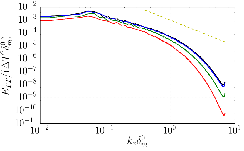
$(b)$

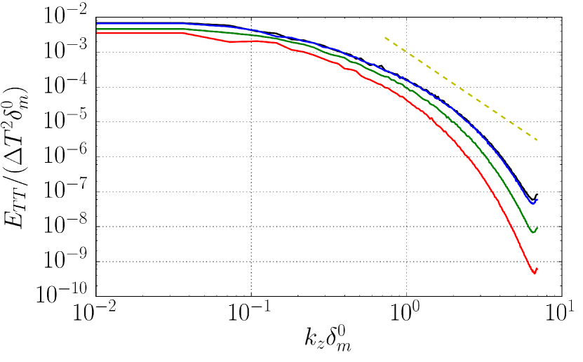
$(c)$

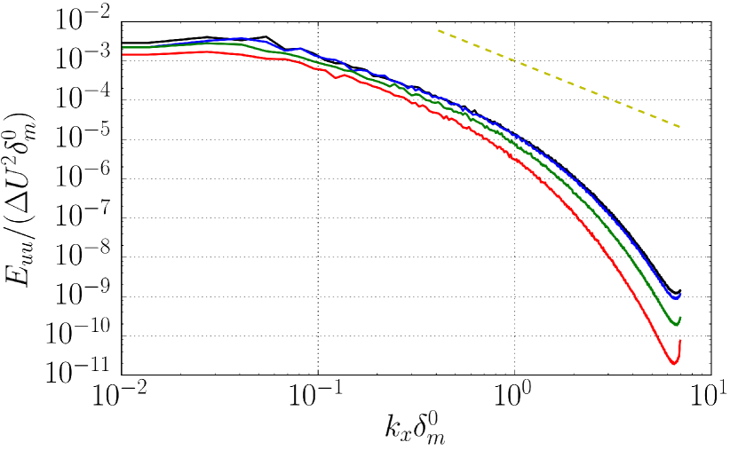
$(d)$

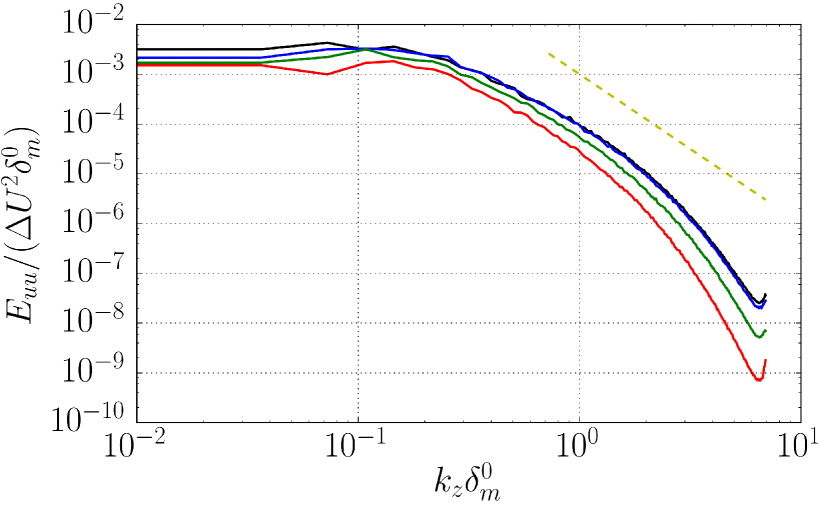
Figure 1: 1D spectra at mid plane of the computational domain ($y=0$), at the beginning of the self-similar range. (a) $E_{TT}(k_{x}\delta_{m}^{0})$. (b) $E_{TT}(k_{z}\delta_{m}^{0})$. (c) $E_{uu}(k_{x}\delta_{m}^{0})$. (d) $E_{uu}(k_{z}\delta_{m}^{0})$. Different colours correspond to different density ratios: black, $s=1$; blue, $s=2$; green, $s=4$ and red, $s=8$.

$s$	$\tau_{0}$ - $\tau_{f}$	$Re_{w}$	$Re_{\lambda}$	$(\Delta x/\eta)_{\max}$	$(\Delta y/\eta)_{\max}$	$D_{w}$
1	380-520	4200-6300	140-150	1.7-1.6	1.1 - 1.05	4.8
2	400-520	4500-5800	130-140	1.6-1.5	1.05 - 0.95	5.2
4	440-620	4500-6500	110-120	1.4-1.3	0.9 - 0.8	6.1
8	550-730	4900-7000	85-95	1.2-0.9	0.7 - 0.6	7.7

Table 1: Relevant parameters of the simulations within self-similar period. All the ranges correspond to the values of the parameter at the beginning ($\tau=\tau_{0}$) and end ($\tau=\tau_{f}$) of the self-similar evolution, discussed in section 4.1. $Re_{w}=\rho_{0}\Delta U\delta_{w}/\mu$, where $\delta_{w}$ is the vorticity thickness. $Re_{\lambda}=q\lambda/\nu$, where $\lambda$ is the Taylor microscale and $q^{2}$ is twice the turbulent kinetic energy. $\Delta x$ and $\Delta y$ are the streamwise and vertical grid spacings in collocation points, respectively. $\eta$ is the Kolmogorov lengthscale. $D_{w}=\delta_{w}/\delta_{m}$, where $\delta_{m}$ is the momentum thickness and $\delta_{w}$ is the vorticity thickness.

4 Results

4.1 Self-similar evolution

It is well known that temporal mixing layers reach a self-similar evolution after an initial transient, in which the initial perturbations evolve into the structure of the fully developed turbulent mixing layer (Rogers and Moser, 1994; Pantano and Sarkar, 2002). In the self-similar evolution, the mixing layer thickness grows linearly with time, and large-scale quantities scaled with the variation across the mixing layer (i.e., $\Delta U$, $\rho_{b}-\rho_{t}$, etc.) collapse into a single profile when plotted as a function of $y/\delta_{m}(t)$ or $y/\delta_{w}(t)$.

In order to evaluate the self-similar evolution of the present DNS results, figure 2(a) shows the evolution of $\delta_{m}(t)$ for the four cases considered here. The variablity in $\delta_{m}$ is estimated using the standard deviation of the momentum thicknesses over the four runs, and is indicated with error-bars in the figure. Also, figure 2(b) shows the time evolution of the integrated dissipation rate of turbulent kinetic energy

$$\zeta=\int_{-\infty}^{\infty}\overline{\varepsilon}dy.$$ (11)

The quantity $\zeta$ scales with $\Delta U^{3}$ and, therefore, should be constant with time, once self-similarity has been achieved. The expression for the dissipation rate of turbulent kinetic energy for variable density flows can be found in Chassaing et al. (2002), and is reproduced here for completeness

$$\overline{\rho}\,\overline{\varepsilon}=\frac{4}{3}\mu\overline{\theta^{\prime 2}}+\mu\overline{\omega^{\prime}_{i}\omega^{\prime}_{i}}+2\mu\left(\frac{\partial^{2}\overline{u^{\prime}_{i}u^{\prime}_{j}}}{\partial x_{i}\partial x_{j}}-2\frac{\partial\overline{\theta^{\prime}u^{\prime}_{j}}}{\partial x_{j}}\right),$$ (12)

where primed variables denote fluctuations with respect to the mean, $\theta=\partial{u_{i}}/\partial{x_{i}}$ is the divergence of the velocity, and $\omega_{i}$ are the components of the vorticity.

The results presented in figure 2 show that self-similarity is achieved after an initial transient, with $\delta_{m}(t)$ growing linearly with time and $\zeta(t)$ becoming approximately constant (at least within the errors in $\zeta$). However, comparing figures 2(a) and 2(b) it can be observed that the linear growth of $\delta_{m}$ starts at $\tau=t\Delta U/\delta_{m}^{0}\approx 200$, a time at which $\zeta$ is still growing. This behavior was also observed by Rogers and Moser (1994), and it indicates that the determination of the time interval where self-similarity is achieved needs a careful consideration, and should not be determined exclusively from a linear evolution of $\delta_{m}(t)$.

$(a)$

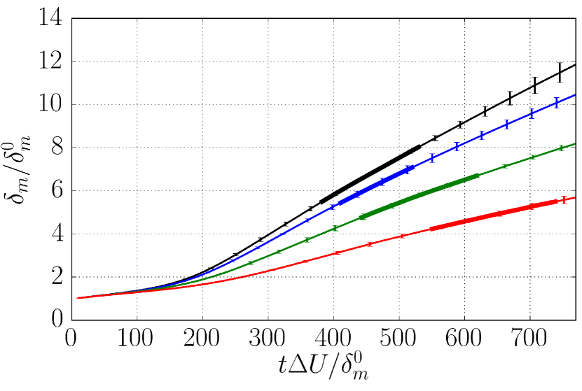
$(b)$

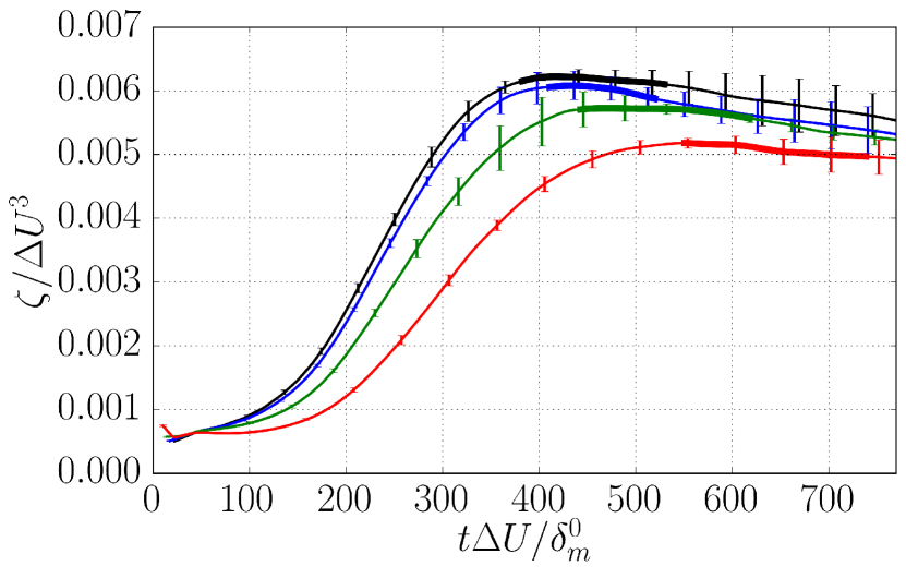
Figure 2: Temporal evolution of (a) the momentum thickness $\delta_{m}$ divided by the initial momentum thickness $\delta_{m}^{0}$, and (b) the non-dimensional integrated turbulent energy dissipation rate, $\zeta/\Delta U^{3}$. Line types are black for $s=1.0$, blue for $s=2.0$, green for $s=4.0$ and red for $s=8$. The values correspond to the ensemble average of the 4 runs for each density ratio, and the error bars are the corresponding standard deviation. The thick line shows the ranges of self-similar evolution for each density ratio.

In the present study, and for the purpose of collecting statistics, we have defined the time interval $[\tau_{0},\tau_{f}]$ where the mixing layer is self-similar by analyzing the collapse of the instantaneous (i.e., averaged in the horizontal directions only) profiles of the normal Reynolds stresses, $R_{11}(y/\delta_{m},\tau)$, $R_{22}(y/\delta_{m},\tau)$, and $R_{33}(y/\delta_{m},\tau)$. We have computed the temporal mean and standard deviation of these Reynolds stresses for several time intervals, selecting for each run the longest time interval in which the standard deviation of the normal Reynolds stresses is smaller than 5% of the maximum. The resulting time intervals (more explicitly, the maximal time interval over the four runs for each density ratio) are shown in figure 2 and reported in table 1, yielding a total self-similar range of at least 10 eddy-turnover times per density ratio. For illustration, figure 3 shows all the $R_{11}$ profiles within the self-similar range for the cases $s=1$ and $s=4$, using different color for each run. The agreement of the profiles is good, especially taking into account that there are 26 and 31 curves on each plot, respectively. The differences are more apparent near the maximum of the Reynolds stresses. It is interesting to note that the variability of the profiles within each run is small, similar to that reported by Pantano and Sarkar (2002). On the other hand, the variability between different runs is a bit larger, and it is probably linked to differences between the largest structures developed in each run (i.e., by different realizations of the initial conditions), emphasizing the importance of running several realizations of each density ratio to accumulate statistics for the largest structures in the mixing layer.

$(a)$

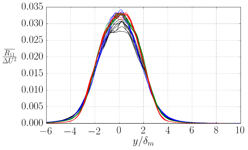
$(b)$

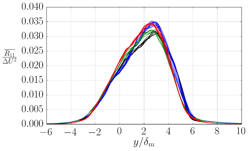
Figure 3: Reynolds stress $R_{11}$ profiles within the self-similar range for (a) case $s=1$, all runs with a total of 26 profiles, and (b) case $s=4$, all runs, with a total of 31 profiles. Colors are used to differentiate between runs.

4.2 Effects of the density ratio on the growth rate

Once the self-similar time interval has been defined, we analyse the effect that the density ratio has on the growth rate of the temporal mixing layer, comparing the results of the present zero Mach cases with those obtained by Pantano and Sarkar (2002) for convective Mach number $M_{c}=0.7$. First, consider the growth rate of the momentum thickness, $\dot{\delta}_{m}$, which is evaluated here following the expression derived in Vreman et al. (1996),

$$\dot{\delta}_{m}\approx-\frac{2}{\rho_{0}\Delta U^{2}}\int_{-\infty}^{\infty}\overline{\rho}R_{12}\cfrac{\partial\tilde{u}}{\partial y}dy.$$ (13)

This expression is obtained differentiating (8) with respect to time, and neglecting viscous terms. An alternative method to compute $\dot{\delta}_{m}$ is to fit a linear law to the data shown in figure 2(a). The differences in the mean and standard deviation of the growth rate of the momentum thickness obtained from both methods are small: for $s=1$, the first method yields $\dot{\delta}_{m}/\Delta U=0.0168\pm 0.0003$, while the second method yields $\dot{\delta}_{m}/\Delta U=0.0170\pm 0.0002$.

The value of the growth rate of the momentum thickness for $s=1$ is in good agreement with previous works, especially taking into account the scatter of the available data. For instance, in the “unforced” experiments quoted by (Dimotakis, 1991b) the growth rate of the momentum thickness varies from 0.014 to 0.022. Also, Rogers and Moser (1994) report $\dot{\delta}_{m}/\Delta U=0.014$ in simulations of incompressible temporal mixing layers, and the experimental data of Bell and Mehta (1990) yield a value of 0.016. For $M_{c}=0.3$ and $s=1$, Pantano and Sarkar (2002) report $\dot{\delta}_{m}/\Delta U\approx 0.0184$, a value that decreases to $0.0108$ when the Mach number is increased to $M_{c}=0.7$.

As the density ratio increases, the values of $\dot{\delta}_{m}$ decrease. This reduction of the growth rate is quantified in figure 4(a), in terms of the ratio of growth rates, $\dot{\delta}_{m}(s)/\dot{\delta}_{m}(1)$. For $s=8$, our results show that the growth rate of $\delta_{m}$ has been reduced by 60% with respect to the growth rate of the case with $s=1$. A similar behaviour is observed for the subsonic cases of Pantano and Sarkar (2002) at $M_{c}=0.7$, also included in the figure. The ratio $\dot{\delta}_{m}(s)/\dot{\delta}_{m}(1)$ is very similar for the $M_{c}=0$ and $M_{c}=0.7$ cases for large density ratios, with significant differences for the smaller density ratio, $s=2$. Careful inspection shows that the density ratio $s=2$ is indeed somewhat anomalous in Pantano and Sarkar (2002), presenting a non-monotonic behaviour for some quantities (see for instance the growth rates and the profiles of Reynolds stress, as shown in table 6 and figure 18 respectively in their paper).

$(a)$

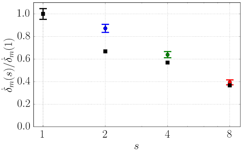
$(b)$

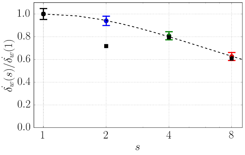
Figure 4: Mixing-layer growth rate as a function of the density ratio. Growth rate based on (a) momentum thickness $\dot{\delta}_{m}$, and (b) vorticity thickness $\dot{\delta}_{w}$, normalised by the growth rate for $s=1.0$. In both panels the horizontal axis is in logarithmic scale. Colored dots with error bars stand for the present results, squares represent results for $M_{c}=0.7$ (Pantano and Sarkar, 2002). The dashed curve in (b) corresponds to equation (14), from Ramshaw (2000).

The results shown in figure 4(a) for $\dot{\delta}_{m}$ are very similar to those obtained for $\dot{\delta}_{w}$, which are plotted in figure 4(b). Again, our results are compared to the $M_{c}=0.7$ cases of Pantano and Sarkar (2002), and the

theoretical prediction by Ramshaw (2000). The latter is based on a model for the growth of the visual thickness of a variable density mixing layer at $M_{c}=0$, directly comparable to the present results. The model is obtained by extending a linear stability analysis to the nonlinear regime through scaling hypothesis, leading after proper manipulation to

$$\frac{\dot{\delta}_{w}(s)}{\dot{\delta}_{w}(1)}=\frac{2\sqrt{s}}{s+1}.$$ (14)

Figure 4(b) shows a very good agreement between Ramshaw’s model and our data. The agreement is also fairly good with the subsonic data of Pantano and Sarkar (2002) at $M_{c}=0.7$, except for the case $s=2$ as it happened also for $\dot{\delta}_{m}$. It should be noted that, to the best of our knowledge, this is the first direct validation of the Ramshaw model with a variable density DNS at $M_{c}=0$.

Overall, the results presented in this subsection show that the growth rates of the $M_{c}=0$ cases are significantly higher than those reported by Pantano and Sarkar (2002) for $M_{c}=0.7$, in agreement with previous works. However, the effect of $s$ on the reduction of the growth rate seems to be very similar at both Mach numbers, except for maybe the low density ratio case, $s=2$. Also, the effect of $s$ seems to be stronger on $\delta_{m}$ than on $\delta_{w}$, with $\dot{\delta}_{m}(s=8)/\dot{\delta}_{m}(s=1)\approx 0.4$ and $\dot{\delta}_{w}(s=8)/\dot{\delta}_{w}(s=1)\approx 0.6$. As a consequence, the ratio between the two thicknesses, $D_{w}=\delta_{w}/\delta_{m}$, increases with $s$, as it can be observed in table 1. Note that since $\delta_{w}$ and $\delta_{m}$ grow linearly with time, $D_{w}\approx\dot{\delta}_{w}/\dot{\delta}_{m}$ for sufficiently long times. For reference, Pantano and Sarkar (2002) report a value of $D_{w}=5.0$ for a compressible mixing layer with $M_{c}=0.3$ and $s=1$, in good agreement with $D_{w}=4.83$ for our $s=1$ case.

4.3 Mean density, velocity and temperature

We now proceed to analyze the one point statistics of the present DNS (mean values in this subsection, higher order moments in §4.4), averaging the data in the horizontal directions and in time, binning in $y/\delta_{m}(t)$. In all the vertical profiles presented in this section, a shadowing has been applied around plus/minus one standard deviation of the horizontally averaged data with respect to the mean, in order to show the uncertainty of the statistics.

$(a)$

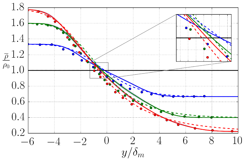
$(b)$

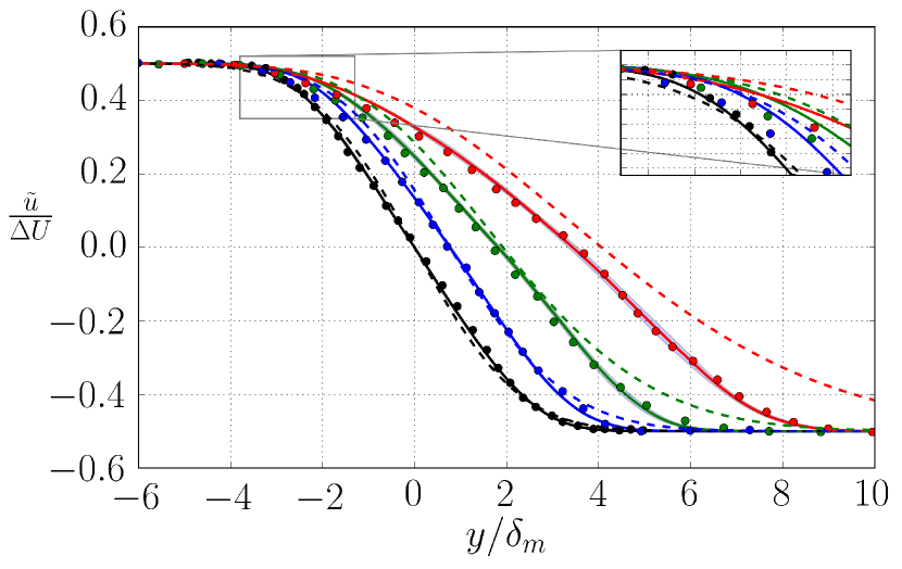
Figure 5: $(a)$ Reynolds-average density profiles. $(b)$ Favre-averaged streamwise velocity profiles. Different colors correspond to different density ratios: black, $s=1$; blue, $s=2$; green, $s=4$; and red, $s=8$. Solid lines are the present turbulent temporal mixing layers. Dashed lines are the laminar temporal mixing layers (see apendix B). Symbols: Rogers and Moser (1994) for $s=1$, Pantano and Sarkar (2002) for s=$2,4$ and 8.

Figure 5(a) shows mean density profiles, comparing the present zero Mach results with the results of the subsonic mixing layer of Pantano and Sarkar (2002) at $M_{c}=0.7$. The figure also includes for comparison the results from laminar temporal mixing layers, obtained as discussed in appendix B. As the density ratio increases, the density mixing layer extends further into the low-density stream, with small variations in the position where $\overline{\rho}=\rho_{0}$. The profiles of the $M_{c}=0.7$ and $M_{c}=0$ cases are qualitatively similar at any given density ratio, although there are some differences in the profiles in the central part of the mixing layer ($\lvert y\rvert\lesssim 3\delta_{m}$). The agreement between the $M_{c}=0$ and $M_{c}=0.7$ cases is better for the Favre averaged velocity, shown in figure 5(b). The only exception is maybe the region closer to the high-density free-stream, where the edge of the mixing layer seems sharper for the present simulations ($M_{c}=0$). The figure also includes the incompressible data of Rogers and Moser (1994) for $s=1$, showing a very good agreement with our incompressible case.

Besides some small changes in the shape of the profiles (which will be discussed later), the most apparent effect of the density ratio in $\overline{\rho}$ and $\tilde{u}$ is the shifting of the $\tilde{u}$ profile towards the low density side. Note that this effect is apparent in both turbulent cases ($M_{c}=0$ and $M_{c}=0.7$), as well as in the laminar self-similar profiles (dashed lines in figure 5). This shifting of the mean density and velocity profiles with the density ratio has already been reported in previous studies, both experimental and numerical, and it has been explained qualitatively in terms of the asymmetry in the momentum exchange of the large scales with the free-streams (Brown and Roshko, 1974) and their linear stability properties (Soteriou and Ghoniem, 1995). Note that the mechanism proposed by Brown and Roshko (1974) acts in both, turbulent diffusion (as originally proposed by the authors) and mean velocity entrainment (i.e, $\langle\rho v\rangle$). While in turbulent mixing layers the turbulent diffusion is dominant over the mean velocity entrainment, the latter is important in laminar mixing layers. This could explain why figure 5 also shows a clear shifting between $\tilde{u}$ and $\overline{\rho}$ for the laminar cases, as well as the results reported by Bretonnet et al. (2007) in laminar mixing layers with density variations due to various effects: different velocities, temperatures or species.

Besides the numerous qualitative observations of the shift between $\tilde{u}$ and $\overline{\rho}$ in the literature, few authors have tried to quantify it. In turbulent mixing layers, Pantano and Sarkar (2002) proposed to quantify this shift using two semi-empirical relationships, $\overline{\rho}(\tilde{u})$ and $R_{12}(\tilde{u})$. They later used these relationships to estimate the reduction of the momentum thickness growth rate. In laminar mixing layers, Bretonnet et al. (2007) proposed to characterize the drift as the distance between the inflection points of the velocity and density mean profiles.

Here we propose to quantify the shift using $\Delta$, which is defined as the distance between the $y$ locations where $\tilde{u}=0$ and $\overline{\rho}=\rho_{0}$, positive when $\tilde{u}$ is displaced towards $y$-positive (low-density side in our simulations). The main advantage of the present definition with respect to those used by Pantano and Sarkar (2002) and Bretonnet et al. (2007) is that it can be easily computed from the mean profiles of velocity and density, without having to compute higher order derivatives. This distance is plotted in figure 6 as a function of the density ratio, for turbulent mixing layers with $M_{c}=0$ and $M_{c}=0.7$, and for the laminar self-similar solutions. The figure shows two possible scalings for $\Delta$, with $\delta_{m}$ (figure 6a) and with $\delta_{w}$ (figure 6b). The different datasets collapse better with the second scaling, especially for $s=8$ cases, suggesting an empirical relation

$$\Delta(s)=\delta_{w}(s)C_{\Delta}\log(s),$$ (15)

with $C_{\Delta}=0.25$. This empirical approximation yields correlation coefficients of $R^{2}=0.998$ for the present DNS results at $M_{c}=0$. Similar values of $C_{\Delta}$ are obtained for the other datasets in the figure. The results of Pantano and Sarkar (2002) at $M_{c}=0.7$ yield $C_{\Delta}=0.23$ and $R^{2}=0.956$, and the laminar self-similar solutions yield $C_{\Delta}=0.23$ and $R^{2}=0.994$. Finally, the good agreement between the laminar and turbulent data (and compressible and low-Mach number data) is consistent with the discussion in the previous paragraphs: the mixing layer is able to erode more easily the lighter free-stream, either by turbulent diffusion (in turbulent mixing layers) or by the mean entrainment (in laminar mixing layers).

$(a)$

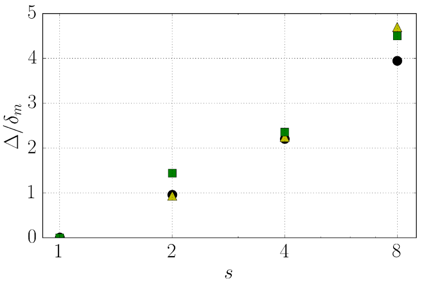
$(b)$

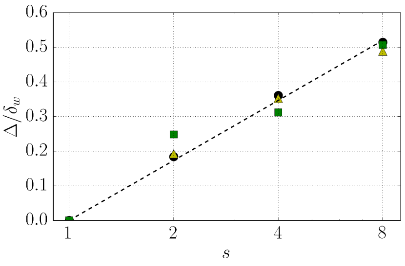
Figure 6: Shifting of the mixing layer, normalized with $(a)$ the momentum thickness, $(b)$ the vorticity thickness. Circles for present DNS at $M_{c}=0$. Squares for Pantano and Sarkar (2002) at $M_{c}=0.7$. Triangles for laminar self-similar solutions. The dashed line in ($b$) corresponds to $\Delta/\delta_{w}=0.25\log(s)$.

Although the present definition of shifting is not directly comparable to the one used by Pantano and Sarkar (2002), it is also possible to relate the present $\Delta$ to the ratio $\delta_{m}(s)/\delta_{w}(s)$. Lets assume that the mean density and velocity profiles are

$$\overline{\rho}=\rho_{0}+\frac{\rho_{t}-\rho_{b}}{2}F_{\rho}\left(\frac{y}{\delta_{w}}\right),\hskip 5.69054pt\mbox{and}\hskip 5.69054pt\tilde{u}=-\frac{\Delta U}{2}F_{u}\left(\frac{y}{\delta_{w}}-\frac{\Delta}{\delta_{w}}\right),$$ (16)

where $F_{u}(\xi)$ and $F_{\rho}(\xi)$ tend to $\pm 1$ when $\xi\to\pm\infty$, and $\Delta$ is assumed to be a function of the density ratio, $s$. Note that this is equivalent to limiting the effect of $s$ to a shift between the profiles of $\overline{\rho}$ and $\tilde{u}$, with no explicit change in their shape. Introducing (16) into (8), it is possible to show that

$$\frac{\delta_{m}(s)}{\delta_{w}(s)}=\frac{\delta_{m}(1)}{\delta_{w}(1)}+\frac{\lambda(s)}{2}\int_{-\infty}^{\infty}\!\!\!F_{\rho}(\xi)\left[1-\left(F_{u}\!\left(\xi-\frac{\Delta}{\delta_{w}}\right)\right)^{2}\right]d\xi=\frac{\delta_{m}(1)}{\delta_{w}(1)}+\lambda(s)G\left(\frac{\Delta}{\delta_{w}}\right),$$ (17)

where $\lambda(s)=(s-1)/(s+1)$. Note that by construction $G(0)=0$ and $G^{\prime}(0)<0$. Hence, it is possible to simplify (17) to

$$\frac{\delta_{m}(s)}{\delta_{w}(s)}=\frac{\delta_{m}(1)}{\delta_{w}(1)}-C\lambda(s)\frac{\Delta}{\delta_{w}}+O\left(\frac{\Delta}{\delta_{w}}\right)^{2}.$$ (18)

Interestingly, piecewise linear expressions for $F_{\rho}$ and $F_{u}$ yield $C=1/3$ and a cubic leading order error in (18).

$(a)$

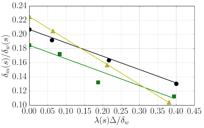
$(b)$

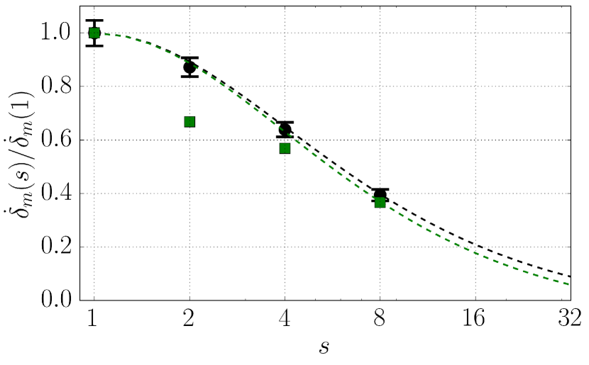
Figure 7: Effects of $s$ and $\Delta$ on the reduction of the momentum thickness. $(a)$ $\delta_{m}/\delta_{w}$ versus $\lambda(s)\Delta/\delta_{w}$. $(b)$ $\dot{\delta}_{m}/\dot{\delta}_{w}$ versus $s$. In both panels, cicles are the present DNS at $M_{c}=0$, squares are Pantano and Sarkar (2002) at $M_{c}=0.7$, and triangles are the self-similar solution for the laminar temporal mixing layer. The solid lines in ($a$) correspond to equation (18) with: black, $C=0.188$; green, $C=0.190$; yellow, $C=0.32$. The dashed lines in ($b$) correspond to (19) with: black, $C^{\prime}=0.047$ and $\dot{\delta}_{w}(1)/\dot{\delta}_{m}(1)=4.8$, green, $C^{\prime}=0.047$ and $\dot{\delta}_{w}(1)/\dot{\delta}_{m}(1)=5.4$.

In order to estimate $C$ from the DNS data, figure 7(a) shows the ratio $1/D_{w}=\delta_{m}/\delta_{w}$ as a function of $\lambda(s)\Delta/\delta_{w}$. The figure shows that $C=0.188$ for the present $M_{c}=0$ data, yielding a correlation coefficient between the data and the linear approximation equal to $R^{2}=0.998$. For the $M_{c}=0.7$ case, the ratio of the growth rates at $s=1$ is smaller, but the slope of the curve seems to be approximately the same ($C=0.190$, $R^{2}=0.920$), supporting the assumption that $F_{\rho}$, $F_{u}$ (and hence $C$) do not vary much with the density ratio. Note that for the laminar case, with notable differences in the shape of $\tilde{u}$ and $\overline{\rho}$ (and hence in $F_{u}$ and $F_{\rho}$), the value of the constant is $C=0.32$ and the linear approximation is exact ($R^{2}=1$).

Finally, it is possible to combine (14), (15) and (18) to obtain a semi-empirical prediction of the reduction of the momentum thickness growth rate with the density ratio,

$$\frac{\dot{\delta}_{m}(s)}{\dot{\delta}_{m}(1)}\approx\frac{2\sqrt{s}}{s+1}\left(1-\frac{\dot{\delta}_{w}(1)}{\dot{\delta}_{m}(1)}C^{\prime}\log(s)\right).$$ (19)

To obtain (19) we have also taken advantage of $1/D_{w}=\delta_{m}/\delta_{w}\approx\dot{\delta}_{m}/\dot{\delta}_{w}$, which is a reasonable approximation for sufficiently long times. The performance of this simple model for the reduction of the momentum thickness growth rate is evaluated in figure 7(b), where the dashed lines corresponds to equation (19) with $C^{\prime}=C\cdot C_{\Delta}=0.047$ and the appropriate value for $\dot{\delta}_{w}(1)/\dot{\delta}_{m}(1)$, black for $M_{c}=0$ and green for $M_{c}=0.7$. The figure also includes the DNS data for both mach numbers. The agreement between the DNS data and the model is very good, except for the lower density ratios of the $M_{c}=0.7$ cases, which already showed differences when compared to the present $M_{c}=0$ cases in figure 4.

$(a)$

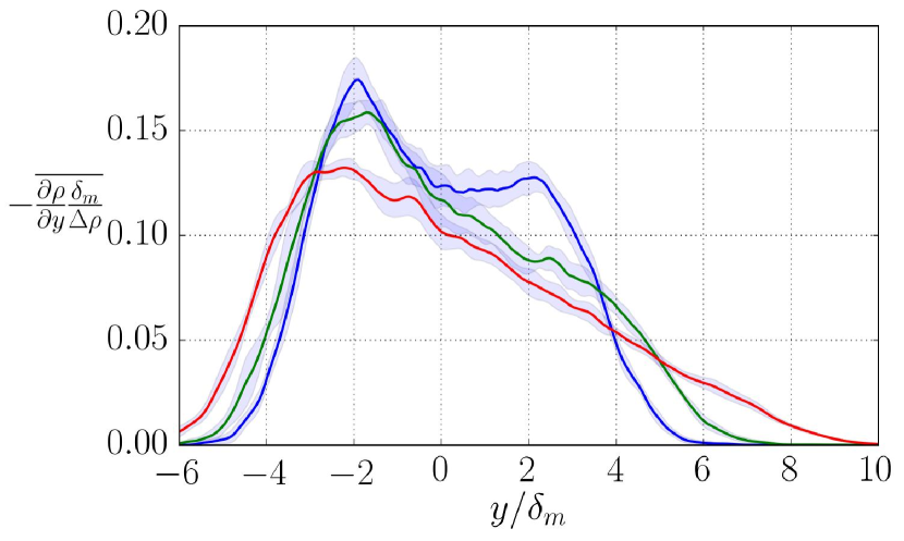
$(b)$

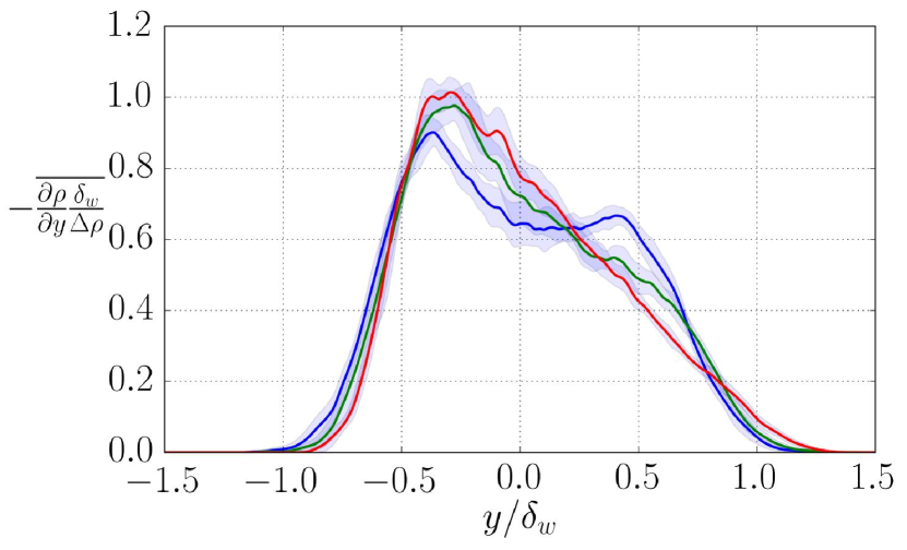
$(c)$

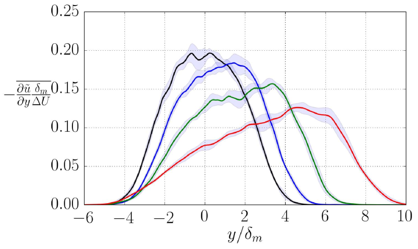
$(d)$

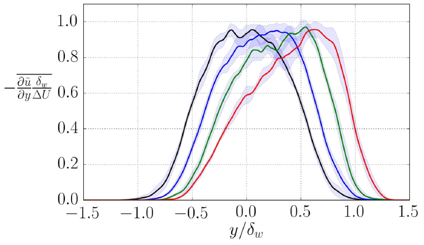
Figure 8: $(a)$,$(b)$ Profiles of the vertical gradients of the Reynolds-averaged density. $(c)$,$(d)$ Profiles of the vertical gradients of the Favre-averaged streamwise velocity. $(a)$,$(c)$ Normalized with the momentum thickness. $(b)$,$(d)$ Normalized with the vorticity thickness. Different colours correspond to different density ratios: black, $s=1$; blue, $s=2$; green, $s=4$; red, $s=8$.

In the previous discussion, the effect of $s$ on the shape of the profiles of $\overline{\rho}$ and $\tilde{u}$ has been neglected, resulting in a reasonable approximation for the reduction in the growth rate of the mixing layer with $s$. However, the density ratio has some effects in the shapes of $\overline{\rho}$ and $\tilde{u}$, which are responsible for changes in the structure of the turbulence in the mixing layer. These effects, which are difficult to evaluate in figure 5, are better observed in figure 8, which shows the vertical gradients of the mean profiles with different normalizations. In particular, the gradients of the mean density normalized with $\Delta\rho=\rho_{b}-\rho_{t}$ and $\delta_{w}$ seem to collapse reasonably well (see figure 8$b$), especially in the high density side (lower stream). More differences are visible near the low density side, where it is apparent that the gradients tend to become smoother with increasing $s$. Indeed, for $s=8$, figure 8$a$ and $b$ show that the gradient of $\overline{\rho}$ is roughly linear, so that $\overline{\rho}$ becomes roughly parabolic for $y\gtrsim-2\delta_{m}\approx-0.25\delta_{w}$. Although outside of the scope of the present paper, it would be interesting to check whether the same linear region in $\partial\overline{\rho}/\partial y$ is obtained for higher density ratios. The shifting of the velocity profiles discussed above is clearly visible when looking at their corresponding gradients, figures 8($c$) and ($d$). For $\tilde{u}$ the change of shape of the profile results in the maximum gradients appearing nearer to the lower density side, with smoother gradients in the high density side. Indeed, opposite to what is observed for $\rho$, case $s=8$ seems to develop a nearly parabolic profile for $\tilde{u}$ towards the higher density side of the mixing layer ($y\lesssim 4\delta_{m}\approx y\lesssim 0.5\delta_{w}$).

To finalize this subsection, we turn our attention to the mean temperature distribution, more especifically to the non-dimensional temperature jump $\overline{\theta}=(\overline{T}-T_{b})/(T_{t}-T_{b})$. It is interesting to study the temperature since it follows an advection-diffusion equation, equation (3). This allows the comparison of the variable density cases ($s=2$, 4 and 8) with the passive scalar simulated for the uniform density case ($s=1$). Note that although the temperature is inversely proportional to the density (equation of state), the same is not true for the mean temperature and mean density. Figure 9(a) shows the mean temperature profiles for all cases and figure 9(b) the corresponding profiles of the vertical gradients of the mean temperature. The passive scalar shows a roughly symmetric distribution, with $\partial\overline{\theta}/\partial y$ peaking near the edges of the mixing layer ($\lvert y/\delta_{w}\rvert\approx 0.5$). The small deviation with respect to a symmetric profile provides an impression about the convergence of the statistics.

With increasing $s$, the mean temperature profiles shifts towards the upper stream (low density stream) in a similar way as the Favre-averaged streamwise velocity. The profiles also become more asymmetric, which is more clearly visible in the mean temperature gradients shown in figure 9(b). As the density ratio increases, the gradients at the high density edge of the mixing layer are strongly damped, while the gradients at the low density edge are enhanced.

$(a)$

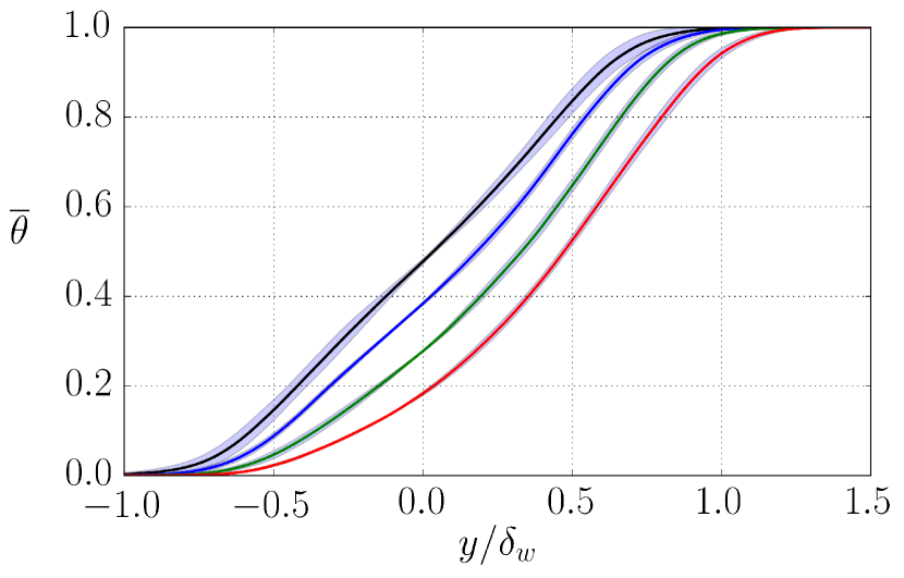
$(b)$

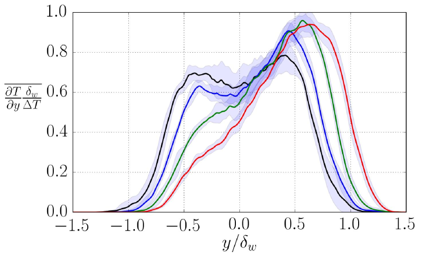
Figure 9: $(a)$ Reynolds-averaged temperature profiles. $(b)$ Profiles of the vertical gradients of the Reynolds-averaged temperature. Different colours correspond to different density ratios: black, $s=1$; blue, $s=2$; green, $s=4$; red, $s=8$.

4.4 Higher order statistics

$(a)$

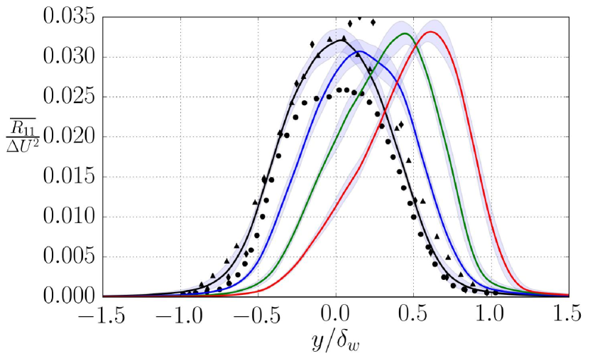
$(b)$

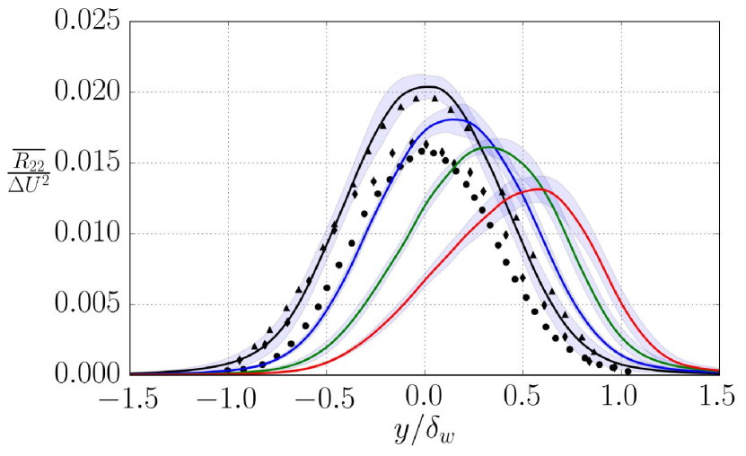
$(c)$

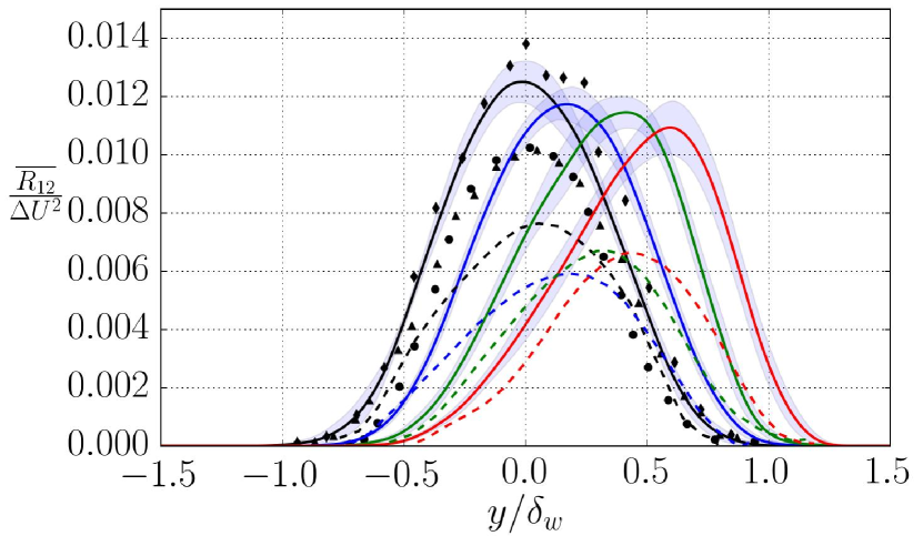
$(d)$

Figure 10: Vertical profiles of (a) $R_{11}/\Delta U^{2}$, (b) $R_{22}/\Delta U^{2}$, (c) $R_{12}/\Delta U^{2}$, and (d) $R_{33}/\Delta U^{2}$. Different colours correspond to different density ratios: black, $s=1$; blue, $s=2$; green, $s=4$; and red, $s=8$. Solid lines are the present turbulent temporal mixing layers. Symbols are data from incompresible mixing layers: dots from simulations of (Rogers and Moser, 1994), triangles from experiments of (Bell and Mehta, 1990) and diamonds from experiments of (Spencer and Jones, 1971). Dashed lines in (c) represent results from $M_{c}=0.7$ (Pantano and Sarkar, 2002).

$(a)$

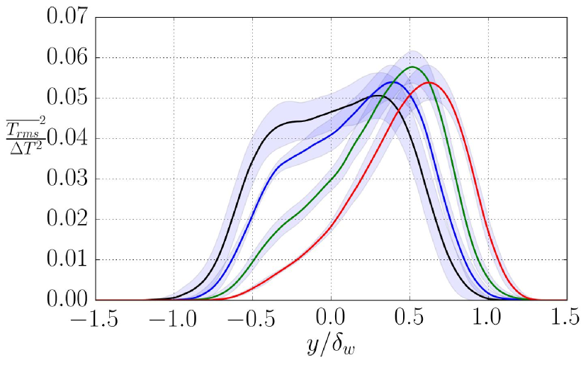
$(b)$

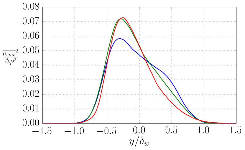
Figure 11: $(a)$ Profiles of $T_{rms}^{2}/\Delta T^{2}$. $(b)$ Profiles of $\rho_{rms}^{2}/\Delta\rho^{2}$. Different colours correspond to different density ratios: black, $s=1$; blue, $s=2$; green, $s=4$; red, $s=8$. Both magnitudes calculated using Reynolds average.

The shifts in the mean velocity and temperature, as well as the changes in their gradients, are also accompanied by changes in the root mean square of velocity and temperature fluctuations, which are analized in figures 10 and 11. In particular, figure 10 displays the vertical profiles of the turbulent stress tensor, $R_{ij}$. The plots include the data for the incompressible mixing layer of Rogers and Moser (1994), and the experimental results of Bell and Mehta (1990) and Spencer and Jones (1971). Both datasets show profiles that are consistent with the shape of the present $s=1$ case, although there is considerable scatter between the three datasets. The scatter in $R_{12}$ (figure 10$c$) is consistent with the scatter in the growth-rates of the mixing layers, since these two quantities are related through equation (13). This could also explain the scatter in $R_{11}$, $R_{22}$ and $R_{33}$ for the cases with $s=1$. As the density ratio increases, $R_{ij}$ tend to shift towards the low-density region, following the maximum gradient of $\tilde{u}$. Interestingly, while the peak values of $R_{22},R_{12}$ and $R_{33}$ decrease with increasing $s$, the peak values of $R_{11}$ seem to remain roughly constant (at least within the uncertainty in the statistics, shown in the figure by the shaded areas around each curve). The high-speed data of Pantano and Sarkar (2002) are also included in figure 10$c$, and they also show a decrease of the peak values of $R_{12}$ with increasing $s$, although for the $M_{c}=0.7$ data the decrease is not monotonic as it is for the present $M_{c}=0$ results. Note also that, as expected, the $M_{c}=0.7$ profiles have lower maximum values, consistent with the lower growth rate of the subsonic mixing layers (as discussed in §4.2 and in Pantano and Sarkar, 2002).

Figure 11 displays the profiles of the variance of the temperature, $T_{rms}^{2}$, and density, $\rho_{rms}^{2}$, normalized with the corresponding jumps across the mixing layer, $\Delta T=T_{t}-T_{b}$ and $\Delta\rho=\rho_{b}-\rho_{t}$, respectively.

For $s=1$ the temperature corresponds to the passive scalar, which exhibits in figure 11(a) the double-peak rms observed in high Reynolds numbers mixing layers by others (e.g., see Pickett and Ghandhi, 2001). When the density ratio is increased, the peak on the high density side gradually decreases, while the peak of $T_{rms}^{2}$ on the low-density side shifts with the mean temperature gradients (see figure 9$b$). This suggests that $T_{rms}^{2}$ is governed by the mean temperature gradient, in a similar way as $\overline{R_{ij}}$ are governed by $\partial\tilde{u}/\partial y$. Indeed, consistent with the mean temperature gradients, the peaks of $T_{rms}^{2}/\Delta T^{2}$ increase with $s$, except for maybe case $s=8$. At the present moment, the reason for the non-monotonous behaviour of $s=8$ is unclear. It could be related to a decrease in the $Re_{\lambda}$ for this case. Another possible explanation could be the onset of interferences of the finite-size of the computational domain with the evolution of the mixing layer.

Not surprisingly, the behaviour of $\rho_{rms}^{2}$ shown in figure 11(b) suggest that $\rho_{rms}^{2}$ is governed by the the mean density gradients (figure 8b), analogous to the behavior of temperature and velocity fluctuations. As $s$ increases, the rms around $y/\delta_{w}\approx-0.5$ (high density side) increases, while the fluctuations around $y/\delta_{w}\approx 0.5$ (low-density side) decrease. The behaviour is opposite to $\overline{R_{ij}}$ (which are more intense near the low density side), which is consistent with the arguments of Brown and Roshko (1974) for the shift and the asymmetry of the growth of the variable density mixing layers.

$(a)$

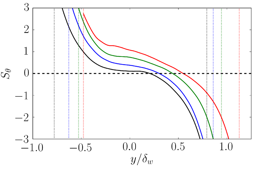
$(b)$

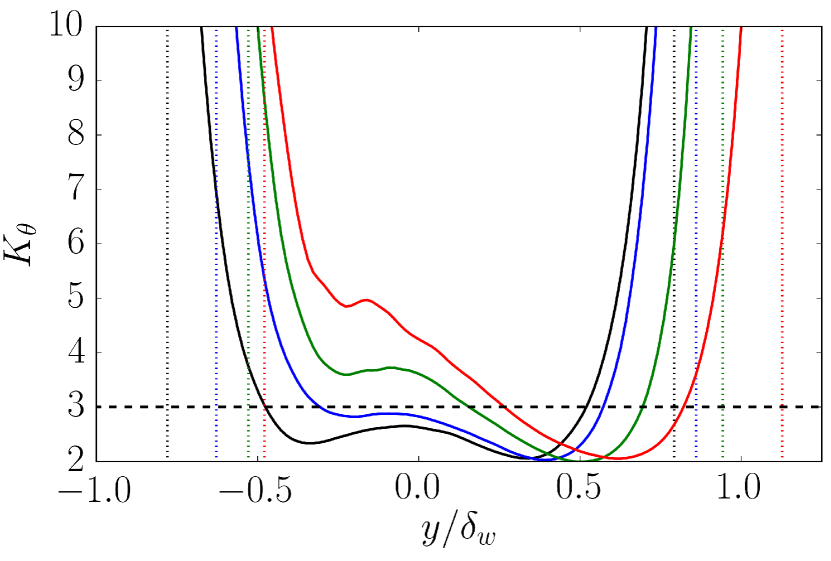
$(c)$

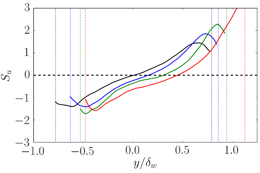
$(d)$

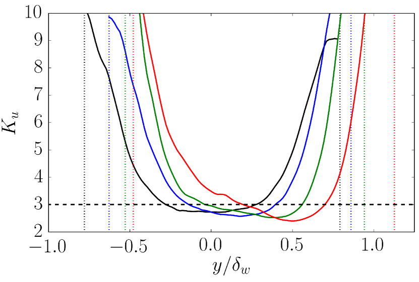
$(e)$

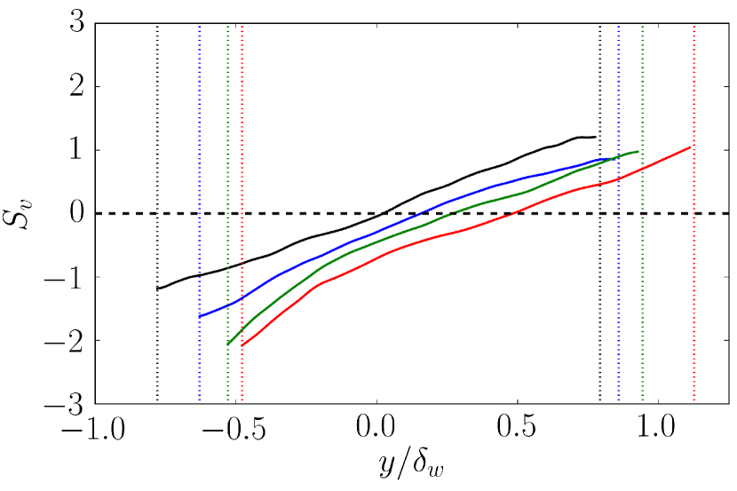
$(f)$

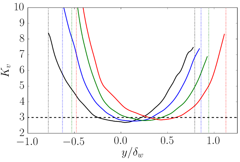
Figure 12: (a) Skewness distribution and (b) Kurtosis distribution of temperature $\theta$; (c) Skewness distribution and (d) Kurtosis distribution of streamwise velocity $u$; (e) Skewness distribution and (f) Kurtosis distribution of vertical velocity $v$. Different colours correspond to different density ratios: black, $s=1$; blue, $s=2$; green, $s=4$; and red, $s=8$.

Finally, figure 12 shows the profiles of the skewness, $S$, and kurtosis, $K$, of the temperature and the velocity field. Since these profiles are more noisy than the second order moments beyond the edge of the mixing layer, figure 12 only shows them in the region limited by 98% of the free stream velocity, indicated with vertical dotted lines. For reference, the horizontal dashed lines represent the expected value for a Gaussian distribution, i.e. $S=0$ and $K=3$. Due to the symmetry of the configuration for the passive scalar case, $s=1$, we expect an antisymmetric distribution for the skewness and a symmetric distribution for the kurtosis. Deviations from this symmetry in figure 12 are small and provide an impression of the convergence of the statistics. Note also that the almost linear profile of $\overline{\theta}$ in the center of the mixing layer results in $S_{\theta}\approx 0$ for the case with $s=1$ (recall the broad maximum of the vertical gradient of $\overline{\theta}$ in figure 9).

Carlier and Sodjavi (2016) measured the skewness and kurtosis in a spatially-developing mixing layer. Their neutral case is comparable to the present passive scalar case. They distinguish between two zones. First, a mixed region in the central part, characterized by a moderate slope of the temperature skewness profile and an almost constant value of all kurtosis profiles. The value of $K$ in this region is somewhat smaller than the Gaussian value. Secondly, the entrained region in the outer part that presents higher slopes of the temperature skewness profile than the mixed, region and also steep gradients of all kurtosis profiles. All these features are clearly observed in the present profiles for the passive scalar case.

Overall, increasing $s$ results in a shift of the profiles of $S$ and $K$ to the low density side, for both temperature and velocity. This is especially clear in $S_{u}$, $S_{v}$ and $K_{v}$, which show small variations on the shape of the profiles (see figures 12$c,e$ and $f$). For the skewness of the temperature (see figure 12$a$) we can observe the same shift, and a gradual increase of $S_{\theta}$ on the high density half of the central region of the mixing layer. This is probably a consequence of the narrowing of the maximum of $\partial\overline{\theta}/\partial y$ with $s$, and its displacement towards the high temperature (low density) side: a sharper edge on the high temperature side makes it more likely for a pocket of high temperature fluid to be entrained into the mixing layer, biasing $S_{\theta}$ towards positive values. It is also interesting to observe that, on top of the shifting, $K_{\theta}$ and $K_{u}$ show some changes in their shape with $s$. In particular, both kurtosis become larger in the high density half of the mixing layer ($y\lesssim 0$). This can be interpreted as an increase in the intermittency of $u$ and $T$, and it suggests that mixing becomes more difficult near the high density region as $s$ increases, in agreement with the qualitative arguments of Brown and Roshko (1974) regarding the reduced velocity fluctuations near the denser stream. As a result, the size of the well mixed region (i.e., with values of $K$ below the Gaussian threshold) is reduced.

4.5 Turbulence structure

Figure 13: Visualization of $\theta$ on an $xy$-plane, at the beginning of the self-similar evolution. The corresponding density ratios and times are (a) $s=1$, $t\Delta U/\delta_{m}^{0}=400$; (b) $s=2$, $t\Delta U/\delta_{m}^{0}=418$; (c) $s=4$, $t\Delta U/\delta_{m}^{0}=455$; and (d) $s=8$, $t\Delta U/\delta_{m}^{0}=570$.

Figure 14: Visualization of $\theta$ on an $xz$-plane at $y=0$, at the beginning of the self-similar evolution. The corresponding density ratios are (a) $s=1$, (b) $s=2$, (c) $s=4$, (d) $s=8$. Times as in figure 13.

Figure 15: Visualization of streamwise velocity on an $xy$-plane, at the beginning of the self-similar evolution. The corresponding density ratios are (a) $s=1$, (b) $s=2$, (c) $s=4$, (d) $s=8$. Times as in figure 13. The black lines show contours of $u=\pm\Delta U/2$.

Figure 16: Visualization of streamwise velocity on an $xz$-plane at $y=0$, at the beginning of the self-similar evolution. The corresponding density ratios are (a) $s=1$, (b) $s=2$, (c) $s=4$, (d) $s=8$. Times as in figure 13.

We provide now visualizations to obtain an impression of the changes in the turbulent structures of the mixing layer induced by the density ratio. Instantaneous fields of the temperature and velocity field are shown using vertical planes (figures 13 and 15 for $\theta$ and $u$, respectively) and horizontal planes (figure 14 and 16 for $\theta$ and $u$ at the plane $y=0$, respectively). Note that, all visualizations correspond to the same time snapshot and same plane locations. For case $s=1$, in which the temperature is a passive scalar, the visualization in figure 13$(a)$ shows the typical features of a turbulent mixing layer, with patches of mixed fluid in the central region alternating with patches of unmixed fluid that are entrained from both streams. The presence of quasi-2D rollers is visible in both temperature (figure 13$a$) and velocity (figure 15$a$) visualizations, but maybe more clearly so in the midplane visualization of the temperature shown in figure 14$(a)$.

On the other hand, the presence of the quasi-2D rollers in the $u$ velocity (figure 15$a$) is masked by the formation of more elongated structures, similar to the streaky structures observed in other free and wall-bounded turbulent shear flows (Lee et al., 1990; Flores and Jiménez, 2010; Sekimoto et al., 2016).

Increasing the density ratio produces small changes in the flow visualizations. The quasi-2D rollers are also observed for $s=2$, 4 and 8 in both temperature (figure 13$b,c$ and $d$) and velocity (figure 15$b,c$ and $d$). Also, in agreement with the results discussed in section 4.3, the mixing layer shifts upwards (towards the low density side) with increasing $s$, as it can be observed in figure 13 and 15. In addition, the temperature field becomes somewhat smoother at the small scales. This fact is reflected in the lower value of $Re_{\lambda}$ obtained in the cases with large $s$, as shown in table 1.

The shift of the mixing layer is also apparent in the visualization of the $y=0$ plane shown in figures 14 and 16. With increasing $s$ the temperature field at this height is increasingly dominated by patches of fluid entrained from the lower stream, while the mean value of the $u$ field drifts to positive values. The footprint of the quasi-2D rollers is also clear in the temperature field (figure 14) for all density ratios, while this footprint becomes less apparent in the $u$ velocity as $s$ increases (figure 16).

Finally, it is interesting to observe in figure 15 that the turbulence within the mixing layer produce irrotational perturbations into the free-stream, with characteristic sizes of the order of $\delta_{w}$. This potential perturbations are relatively weak, and are highlighted in figure 15 by contours of $u=\pm\Delta U$ (in black).

In order to quantify the changes in the structure of the turbulent motions in the mixing layer due to the density ratio, we proceed to analyse the one dimensional spectra of velocity and temperature fluctuations: $E_{ii}(k_{x},y)$ and $E_{ii}(k_{z},y)$ for $i=u,v$ and $T$ (no summation). These spectra are computed during runtime, as functions of $k_{x}\delta_{m}^{0}$, $k_{z}\delta_{m}^{0}$, $y/\delta_{m}^{0}$ and $t$. Then, during post-processing, these spectra are interpolated into wavenumbers and vertical distances normalized with $\delta_{w}(t)$, and averaged (ensemble and in time) for the self-similar evolution of the mixing layer. The smallest wavenumbers considered in the interpolation are $k_{x}^{0}\delta_{w}\approx 0.4-0.5$ and $k_{z}^{0}\delta_{w}\approx 1.1-1.3$, depending on the density ratio.

Figure 17 shows the premultiplied spectra ($k_{x}E_{ii}$ and $k_{z}E_{ii}$), as a function of the vertical position in the mixing layer and the streamwise or spanwise wavelength, $\lambda_{x}=2\pi/k_{x}$ and $\lambda_{z}=2\pi/k_{z}$. The spectra is premultiplied by the wavenumber so that, when plotted in log-scale for the wavelength, the area under the surface corresponds to the actual energy content of a given range of wavelengths. The contours plotted in the figure correspond to 20% and 40% of the maxima among all cases, so that they represent equal levels of energy density for all cases. The small inset to the right of each panel shows the energy in wavenumbers smaller than $k_{x}^{0}$ and $k_{z}^{0}$,

$$E_{ii}^{L}(y)=\sum_{k_{x}=0}^{k_{x}^{0}}E_{ii}(k_{x},y)\hskip 11.38109pt\mbox{and}\hskip 11.38109ptE_{ii}^{W}(y)=\sum_{k_{z}=0}^{k_{z}^{0}}E_{ii}(k_{z},y).$$ (20)

From a physical point of view, these two quantities roughly corresponds to the energy in structures that are infinitely long ($E_{ii}^{L}$) or wide ($E_{ii}^{W}$).

$(a)$

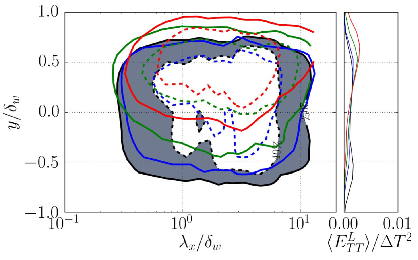
$(b)$

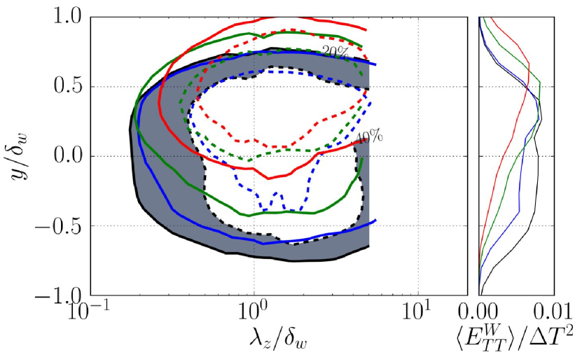
$(c)$

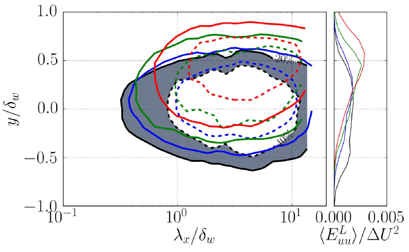
$(d)$

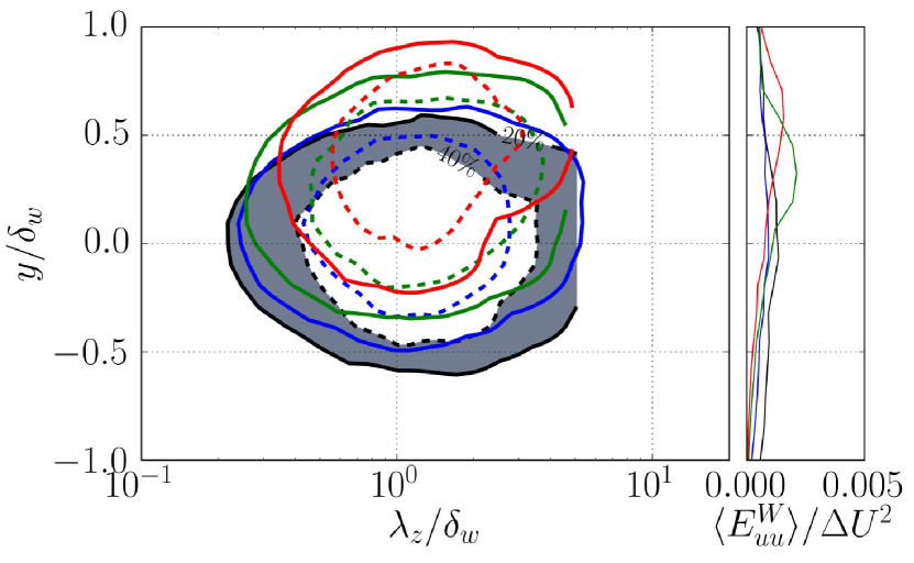
$(e)$

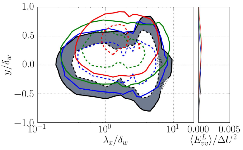
$(f)$

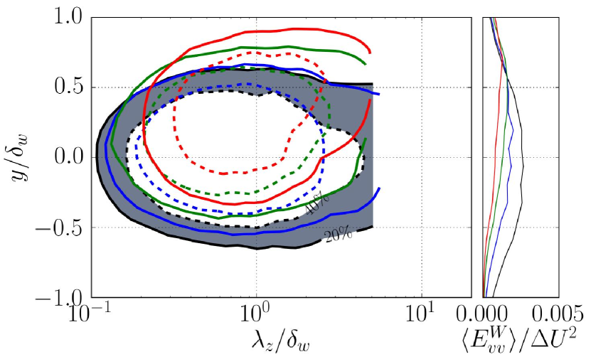
Figure 17: Vertical distribution of the premultiplied spectral energy distribution of velocity and temperature. (a) $k_{x}E_{TT}(\lambda_{x},y)$. (b) $k_{z}E_{TT}(\lambda_{z},y)$. (c) $k_{x}E_{uu}(\lambda_{x},y)$. (d) $k_{z}E_{uu}(\lambda_{z},y)$. (e) $k_{x}E_{vv}(\lambda_{x},y)$. (f) $k_{z}E_{vv}(\lambda_{z},y)$. The inset to the right of each panel shows the energy in wavenumbers not included in the corresponding panel (see text for discussion). The contours plotted correspond to 20% (solid) and 40%(dashed) of the maxima of all the spectra shown in each panel. Different colours correspond to different density ratios: black with shading, $s=1$; blue, $s=2$; green, $s=4$ and red, $s=8$.

For the incompressible case, figure 17 shows that the spectra of $u$ tend to be longer than wide, while the spectra of $v$ and $T$ tend to be wider than long, consistently with the visualizations shown in figures 14 and 16. Indeed, both $T$ and $v$ show considerably more energy on structures that are wide ($\lambda_{z}>2\pi/k_{z}^{0}\approx 5\delta_{w}$) than in structures that are long ($\lambda_{x}>2\pi/k_{x}^{0}\approx 12\delta_{w}$), which is shown by $E_{vv}^{W}>E_{vv}^{L}$ and $E_{TT}^{W}>E_{TT}^{L}$. It is also apparent in figure 17 that the spectra of $v$ is shifted towards smaller scales with respect to the spectra of $u$ and $T$, both in $\lambda_{x}$ and $\lambda_{z}$. In terms of the vertical extension of the spectra, 17($a$) and ($b$) show that the temperature spreads over $\lvert y\rvert\lesssim 0.8\delta_{w}$, while $u$ and $v$ are limited to a narrower region ($\lvert y\rvert\lesssim 0.5\delta_{w}$), in agreement with the results shown in figure 10. Interestingly, figure 17($e$) shows that $E_{vv}$ has a larger spread in the vertical direction, at about $\lambda_{x}\approx 4\delta_{w}$. Careful inspection of figures 17($e$) and ($f$) shows that those peaks correspond to infinitely wide structures ($k_{z}=0$): note that $E_{vv}(\lambda_{z},y)$ at $y=0.7\delta_{w}$ has little energy (i.e., below the 20% contour), while $E_{vv}^{W}$ at the same height is still important (i.e., around 50% of the maximum of $E_{vv}^{W}$).

Although not shown here, instantaneous visualizations of $v$ show that these wavelengths ($\lambda_{x}\approx 4\delta_{w}$, $\lambda_{z}\to\infty$) roughly correspond to potential perturbations of $v$ into the free-stream, analogous to the potential perturbations of $u$ highlighted in figure 15.

As the density ratio increases, figures 17($a$) and ($b$) show that the spectra of the temperature gradually shifts towards the low density side (see the contours of 20% in the figures). The shift occurs first on the high density edge of the spectrum ($y<0$), and a bit later in low density side ($y>0$). Note that for $y/\delta_{w}\gtrsim 0.25$, there are little differences between the spectra of the $s=1$ and $s=2$ cases, consistent with the agreement of $T_{rms}^{2}$ in figure 10($d$) in these same vertical locations. In terms of the effect of $s$ in the streamwise and spanwise wavelengths, figure 17($a$) shows that the longest scales in the high density side are gradually inhibited ($\lambda_{x}/\delta_{w}\approx 5-10,y\approx 0$). The same effect, although weaker, is also present in the spanwise wavelengths (figure 17$b$). In terms of the small scales, figures 17($a$) and ($b$) suggest that the effect of $s$ is stronger on $\lambda_{z}$ than on $\lambda_{x}$. This could be related to the fact that the small scales in $x$ are not only due to turbulent fluctuations (i.e., vortices), but to the formation of sharp gradients $\partial T/\partial x$, due to the roll-up of the shear layer (see blue lines in figures 13 and 14).

The behaviour of the spectra of $u$ and $v$ in figures 17($c-f$) is qualitatively similar to that discussed for $T$, with all spectra shifting towards the low-density side, with a gradual reduction of the energy in small scales (both $\lambda_{x}$ and $\lambda_{z}$). There is also a clear reduction of the energy of large scales near the high-density edge of the mixing layer, more apparent for wide ($\lambda_{z}/\delta_{w}\gtrsim 3-5$) structures than for long structures ($\lambda_{x}/\delta_{w}\gtrsim 5-10$). The $u$ and $v$ spectra of cases $s=1$ and $s=2$ also agree reasonably well near the low-density edge of the mixing layer ($y\gtrsim 0.25\delta_{w}$), except for the $v$ spectrum at about $\lambda_{x}\approx 4\delta_{w}$, suggesting that even a small change on the density ratio has an important effect on the potential perturbations of the mixing layer into the free-stream.

5 Conclusions

In this paper we have presented results from direct numerical simulations of temporal, turbulent mixing layers with variable density. The simulations are performed in the low-Mach number limit, so that temperature and density fluctuations develop while the thermodynamic pressure remains constant. Four different density ratios are considered, $s=1$, 2, 4 and 8, which are run in large computational boxes until they reach an approximate self-similar evolution. To give an impression of the turbulence in these mixing layers, during the self-similar evolution the Reynolds numbers based on the Taylor micro-scale vary between $Re_{\lambda}=$ 140-150 for the case $s=1$, and $Re_{\lambda}=$ 85-95 for the case with the highest density ratio, $s=8$.

The results of the simulations show that, in agreement with turbulent mixing layers with higher velocities (and convective Mach number, $M_{c}=0.7$), the growth rate of the momentum thickness decreases with the density ratio. Note that at a given density ratio, the momentum thickness of the low-Mach number mixing layer will grow faster than the subsonic one. However, the ratio between the growth rate for large density ratios and the growth rate of the $s=1$ case seems to be independent of the flow speed in the range considered. For example, for $s=8$ a 60% growth reduction with respect to $s=1$ is obtained for both the present low Mach number case and the $M_{c}=0.7$ case.

In terms of the visual thickness of the mixing layer, the effect of the density ratio in the growth reduction with respect to the $s=1$ case is smaller, and our results agree with previous theoretical models for $M_{c}=0$ and with the data of high-speed mixing layers. However, the growth rate reduction for low density ratio ($s=2$) is not the same in the $M_{c}=0$ and in the $M_{c}=0.7$ cases from Pantano and Sarkar (2002). This discrepancy could mean that compressibility effects are more dominant for low density ratios, but additional analysis of the subsonic cases is required to confirm this conjecture.

The Favre averaged profiles of velocity show that with increasing density ratio, the gradients shift towards the low density side. The behaviour is analogous to that observed in high-speed mixing layers. Indeed, the velocity and density profiles of our low-Mach number cases agree qualitatively well with the high-speed cases when the vertical distance is normalised with $\delta_{m}$. There are some small differences in the mean velocities near the low density stream, and the density profiles of the high-speed cases seem to be displaced with respect to the low-Mach number profiles.

We have quantified the shifting of the Favre-averaged velocity profiles with respect to the density profiles as the distance ($\Delta$) between the locations where velocity and density are equal to the mid value between the free-streams. Using our data, we have also obtained an empirical relationship between $\Delta$ and $s$, which we have used to obtain a semi-empirical model for the reduction of momentum thickness growth rate with the density ratio, see equation (19). This model uses the theoretical prediction of the reduction of the vorticity thickness growth rate due to Ramshaw (2000). From a physical point of view, the model assumes that the only effect of the density ratio is a shift in the velocity profile, with no change on the shape of the density and velocity profiles. Our data for $M_{c}=0$ and the data of Pantano and Sarkar (2002) for $M_{c}=0.7$ are in good agreement with the model prediction, except for maybe the $M_{c}=0.7$ case at low density ratios ($s\approx 2$). It would be interesting to check the validity of the model prediction for higher density ratios.

The fluctuation profiles of the low-Mach number cases show that, as expected, the fluctuations follow the gradients.

While velocity and temperature shift towards the low-density region, density fluctuations and gradients seem to concentrate near the high-density edge of the mixing layer, consistently with the quantitative arguments of Brown and Roshko (1974) for the asymmetric growth of variable density mixing layers.

The analysis of the skewness and the kurtosis of the fluctuations shows that increasing the density ratio, the well mixed region that appears in the central region of the case $s=1$ becomes narrower, since mixing becomes more difficult near the high density side as the density ratio is increased.

Finally, the flow structures have been analyzed using flow visualizations and premultiplied spectra. The spectra shows that with increasing density ratio there is a shift of the turbulent structures towards the low density side, while the longest scales in the high density side are gradually inhibited. A gradual reduction of the energy in small scales with increasing density ratio is also observed. This effect is consistent with the reduction of $Re_{\lambda}$ with increasing density ratio mentioned above.

Appendix A Numerical method

In this section, we describe the equations and algorithms implemented in the in-house code employed in this work for solving temporal mixing layers under the low-Mach number approximation. The governing equations for a variable-density flow with constant fluid properties under the low-Mach number approximation can be written in the following dimensionless form,

$$\cfrac{\partial\rho}{\partial t}+\cfrac{\partial(\rho u_{i})}{\partial x_{i}} =0,$$ (21)

$$\cfrac{\partial(\rho u_{i})}{\partial t}+\cfrac{\partial(\rho u_{i}u_{j})}{\partial x_{j}} =-\cfrac{\partial p^{(1)}}{\partial x_{i}}+\frac{1}{Re}\cfrac{\partial\tau_{ij}}{\partial x_{j}},$$ (22)

$$\cfrac{\partial T}{\partial t}+u_{i}\cfrac{\partial T}{\partial x_{i}} =\frac{T}{Pe}\nabla^{2}{T},$$ (23)

$$\rho T =1,$$ (24)

where, all variables are non-dimensionalized by the initial momentum thickness $\delta_{m}^{0}$, the characteristic velocity $\Delta U$ and the physical magnitudes at the reference temperature, $T_{0}$, and pressure, $p^{(0)}=\rho_{0}RT_{0}$, namely $\rho_{0}$, $\mu$, $C_{p}$ and $\kappa$. Therefore, the dimensionless numbers appearing here are defined as,

$$Re=\frac{\rho_{0}\Delta U\delta_{m}^{0}}{\mu},$$ (25)

$$Pe=\frac{\rho_{0}C_{p}\Delta U\delta_{m}^{0}}{\kappa}=PrRe.$$ (26)

Note that $p^{(1)}$ in eq. (22) is the mechanical pressure, different from the thermodynamic pressure, $p^{(0)}$, as discussed in the introduction. In order to eliminate the mechanical pressure $p^{(1)}$ from the equations, first a Helmholtz decomposition is applied to the momentum vector

$$\rho\vec{u}=\vec{m}+\nabla\psi,$$ (27)

with $\vec{m}$ being a divergence-free component, so that

$$\cfrac{\partial m_{x}}{\partial x}+\cfrac{\partial m_{y}}{\partial y}+\cfrac{\partial m_{z}}{\partial z}=0,$$ (28)

and $\nabla\psi$ is a curl-free component. Similar to the formulation developed by Kim et al. (1987) for incompressible flow, we define

$$\phi =\nabla^{2}m_{y},$$ (29)

$$\Omega_{y} =\left.\nabla\times\vec{m}\right|_{y}=\cfrac{\partial m_{x}}{\partial z}-\cfrac{\partial m_{z}}{\partial x}.$$ (30)

The evolution equations for these two variables are obtained by proper manipulation of eqs. (21-22). This leads to a system of four evolution equations for the variables $\phi$, $\Omega_{y}$, $T$ and $\rho$ together with the equation of state (24),

$$\frac{\partial{\phi}}{\partial t} =F(\rho,u_{j})=\cfrac{\partial^{2}N_{y}}{\partial x^{2}}+\cfrac{\partial^{2}N_{y}}{\partial z^{2}}-\cfrac{\partial}{\partial y}\left({\cfrac{\partial N_{x}}{\partial x}}+{\cfrac{\partial N_{z}}{\partial z}}\right)-\frac{1}{Re}\left.\nabla^{2}({\nabla\times\vec{\omega}})\right|_{y},$$ (31)

$$\cfrac{\partial\Omega_{y}}{\partial t} =M(\rho,u_{j})=\cfrac{\partial N_{x}}{\partial z}-\cfrac{\partial N_{z}}{\partial x}+\frac{1}{Re}\left({\nabla^{2}\omega_{y}}\right),$$ (32)

$$\cfrac{\partial T}{\partial t} =E(\rho,u_{j})=-\vec{u}\cdot\nabla T+\frac{T}{Pe}\nabla^{2}{T},$$ (33)

$$\cfrac{\partial\rho}{\partial t} =C(\rho,u_{j})=-\nabla\cdot(\rho\vec{u})=-\nabla^{2}\psi,$$ (34)

where $N_{i}=-\partial(\rho u_{i}u_{j})/\partial x_{j}$ and $\vec{\omega}$ is the vorticity.

The manipulations to obtain eqs. (31-32) involve taking spatial derivatives of the momentum equations. In this process, information concerning the horizontally averaged momentum vector is lost, requiring additional equations to keep this effect. Averaging eq. (22) over the homogeneous directions $x$ and $z$, we obtain equations for $\langle\rho u\rangle$ and $\langle\rho w\rangle$,

$$\cfrac{\partial\langle\rho u\rangle}{\partial t} =-\cfrac{\partial\langle\rho uv\rangle}{\partial y}+\cfrac{1}{Re}\cfrac{\partial\langle\tau_{xy}\rangle}{\partial y},$$ (35)

$$\cfrac{\partial\langle\rho w\rangle}{\partial t} =-\cfrac{\partial\langle\rho vw\rangle}{\partial y}+\cfrac{1}{Re}\cfrac{\partial\langle\tau_{zy}\rangle}{\partial y}.$$ (36)

Averaging eq. (21) over the homogeneous directions $x$ and $z$ and integrating in $y$ we obtain an equation for $\langle\rho v\rangle$,

$$\int_{-\infty}^{y}\cfrac{\partial\langle\rho\rangle}{\partial t}dy=-\int_{-\infty}^{y}\cfrac{\partial\langle\rho v\rangle}{\partial y}dy=\langle\rho v\rangle_{b}-\langle\rho v\rangle(y).$$ (37)

Note that $\langle\rho u\rangle,\langle\rho v\rangle$ and $\langle\rho w\rangle$ correspond to the $k_{x}=0$ and $k_{z}=0$ modes of the Fourier expansions in $x$ and $z$. These variables are in principle functions of $y$ and $t$.

The algorithm to solve eqs. (31-34) is split into two parts. First, we employ an explicit, low-storage, 3-stage Runge-Kutta scheme for eqs. (31-33), that for the $i$-th stage reads

$$\phi^{i} = \phi^{i-1}+\gamma_{i}\Delta tF(\rho,u_{j})^{i-1}+\epsilon_{i}\Delta tF(\rho,u_{j})^{i-2},$$

$$\Omega_{y}^{i} = \Omega_{y}^{i-1}+\gamma_{i}\Delta tM(\rho,u_{j})^{i-1}+\epsilon_{i}\Delta tM(\rho,u_{j})^{i-2},$$

$$T^{i} = T^{i-1}+\gamma_{i}\Delta tE(\rho,u_{j})^{i-1}+\epsilon_{i}\Delta tE(\rho,u_{j})^{i-2},$$ (38)

where $\gamma_{i}=(8/15,5/12,3/4)$ and $\epsilon_{i}=(0,-17/60,-5/12)$ are the coefficients of the explicit scheme (Spalart et al., 1991). For eq. (34) we employ an implicit, low-storage, 3-stage Runge-Kutta scheme, that for the $i$-th stage reads

$$\rho^{i}=\rho^{i-1}-\Delta t\left(\alpha_{i}\nabla^{2}\psi^{i-1}+\beta_{i}\nabla^{2}\psi^{i}\right),$$ (39)

where $\alpha_{i}=(5/66,17/15,1/22)$ and $\beta_{i}=(151/330,-1,19/66)$ are the coefficients of the implicit scheme, optimized to enhance the stability of the code in a similar way as Jang and de Bruyn Kops (2007). Note that this equation is a Poisson problem for $\psi^{i}$ if $\rho^{i}$ is known. However, from the point of view of mass conservation, it is beneficial to express $\rho^{i}-\rho^{i-1}$ in terms of the temperature, and use the fact that $\nabla^{2}\psi=-\partial\rho/\partial t=T^{-2}\partial T/\partial t=T^{-2}E(\rho,u_{j})$ , yielding

$$\nabla^{2}\psi^{i}=\frac{1}{\beta_{i}\Delta t}\frac{T^{i}-T^{i-1}}{T^{i}T^{i-1}}-\frac{\alpha_{i}}{\beta_{i}}\left(\frac{E(\rho,u_{j})}{T^{2}}\right)^{i-1}.$$ (40)

With this formulation, we are assuring that the energy equation acts as a constraint for the continuity equation (as suggested by Nicoud, 2000), keeping both equations synchronised at every time step.

From eq. (38) we obtain $\phi^{i}$, $\Omega_{y}^{i}$ and $T^{i}$. Using eq. (24) we obtain $\rho^{i}$, and solving the Poisson problem (39) we obtain $\psi^{i}$. In order to compute the right hand side of eqs. (31-33) the velocity and the vorticity are needed. The velocity is constructed as follows. First, knowing $\phi$ we solve the Poisson problem eq. (29) to obtain $m_{y}$. Knowing $\Omega_{y}$, we can solve eqs. (28) and (30) to obtain $m_{x}$ and $m_{z}$. Finally, knowing $\psi$ and $\rho$, from the definition, eq. (27), we obtain the velocity field and by differentation the vorticity field.

A.1 Boundary conditions: entrainment

As discussed in the main text, the velocity and density fluctuations should tend to zero as $y\rightarrow\pm\infty$. We impose

$$\begin{array}[]{llll}\rho=\rho_{b},&u=\Delta U/2,&w=0&\mbox{ at }y\rightarrow-\infty,\\ \rho=\rho_{t},&u=-\Delta U/2,&w=0&\mbox{ at }y\rightarrow\infty.\end{array}$$ (41)

Due to the entrainment there is a non-zero value of $\langle\rho v\rangle$ at $y\rightarrow\pm\infty$. Integrating eq. (37) from $-\infty$ to $\infty$ we obtain the total mass outflow, $\Phi$, as

$$\Phi=\int_{-\infty}^{\infty}\cfrac{\partial\langle\rho\rangle}{\partial t}dy=\langle\rho v\rangle_{b}-\langle\rho v\rangle_{t}.$$ (42)

It is possible to express the total mass outflow as a function of the vertical entrainment ratio, $E_{v}=-\langle v\rangle_{b}/\langle v\rangle_{t}$, as

$$\Phi=\langle\rho v\rangle_{b}\left(1+\frac{1}{E_{v}s}\right).$$ (43)

Dimotakis (1986) suggests that, for a variable-density temporal mixing layer, the entrainment ratio should be equal to the square root of the density ratio, an argument attributed to Brown (1974). Using this result and computing during runtime the value of $\Phi$ we obtain $\langle\rho v\rangle_{b}$ from eq.(43) and $\langle\rho v\rangle_{t}=\langle\rho v\rangle_{b}-\Phi$. Note that during the self-similar evolution, since $\rho$ should scale with $\rho_{b}-\rho_{t}$ and the thickness of the layer grows linearly with time, the value of $\Phi$ should remain constant. Therefore, during the self-similar evolution the values of $\langle\rho v\rangle_{t}$ and $\langle\rho v\rangle_{b}$ should be constant as well.

Appendix B Variable density laminar mixing layer: self-similar solution

In this appendix we present the procedure followed to obtain a self-similar solution for a laminar temporal mixing layer. The configuration is the same discussed in the body of the paper for the turbulent mixing layer: two opposing streams with a velocity difference $\Delta U$ and a density ratio $s$. The differences with respect to equations (1-4) is that the spanwise velocity is $w=0$, and that the rest of the fluid variables are only functions of the vertical coordinate, $y$, and time, $t$. Then, the equations governing the problem are

$$\cfrac{\partial\rho}{\partial t}+\cfrac{\partial\rho v}{\partial y} =0$$ , (44)

$$\cfrac{\partial u}{\partial t}+v\cfrac{\partial u}{\partial y} =T\frac{\mu}{\rho_{0}T_{0}}\cfrac{\partial^{2}u}{\partial y^{2}}$$ , (45)

$$\cfrac{\partial T}{\partial t}+v\cfrac{\partial T}{\partial y} =T\frac{k}{\rho_{0}C_{p}T_{0}}\cfrac{\partial^{2}T}{\partial y^{2}}$$ , (46)

plus the equation of state $\rho T=\rho_{0}T_{0}$. In these equations $\mu$ is the dynamic viscosity, $\kappa$ is the thermal conductivity and $C_{p}$ is the specific heat at constant pressure. Note that the vertical component of the momentum equation is not included, since it introduces an additional unknown, the mechanical pressure $p^{(1)}(y,t)$. The boundary conditions are the same as for the turbulent mixing layer, with velocity and density (temperature) going to the free-stream values when $y\to\pm\infty$.

In order to solve the system of coupled partial differential equations given by (44-46) we define the density-weighted vertical coordinate,

$$\xi=\frac{1}{\rho_{0}}\int_{-\infty}^{y}\rho dy.$$ (47)

We also define a characteristic length for the problem, based on the kinematic viscosity ($\nu=\mu/\rho_{0}$) and time, $\delta=\sqrt{\nu t}$. Then, using $\xi$ and $\delta$ it is possible to recast equations (44-46) into a self-similar set of equations in which the time dependence is absorbed into the self-similar coordinate $\eta=\xi/\delta$,

$$\frac{\partial V}{\partial\eta}+\frac{\eta}{2}\frac{\partial\Theta}{\partial\eta} =0$$ , (48)

$$\frac{\partial U}{\partial\eta}\frac{\eta}{2}+\frac{\partial}{\partial\eta}\left(\frac{1}{\Theta}\frac{\partial U}{\partial\eta}\right) =0$$ , (49)

$$\frac{\partial\Theta}{\partial\eta}\frac{\eta}{2}+\frac{1}{Pr}\frac{\partial}{\partial\eta}\left(\frac{1}{\Theta}\frac{\partial\Theta}{\partial\eta}\right) =0$$ , (50)

where $U=u/\Delta U$, $V=v/\sqrt{\nu/t}$, $\Theta=T/T_{0}$ and $Pr$ is the Prandtl number. The boundary conditions for $U(\eta)$ and $\Theta(\eta)$ are $U(\pm\infty)=\mp 0.5$, $\Theta(+\infty)=(1+s)/2$ and $\Theta(-\infty)=(1+1/s)/2$. Interestingly, in the self-similar set of equations, $V$ appears only in the continuity equation, allowing to solve for $U(\eta)$ and $\Theta(\eta)$ using the momentum and energy equations only. Unfortunately, the equations only admit analytical solution when $s=1$. For other values of $s$, equations (49) and (50) are solved together using Chebychev polynomials (Driscoll et al., 2008).

References

- Ashurst and Kerstein [2005] Wm. T. Ashurst and A. R. Kerstein. One-dimensional turbulence: Variable-density formulation and application to mixing layers. Phys. Fluids, 17:025107, 2005. doi: 10.1063/1.1847413.
- Bell and Mehta [1990] J. H. Bell and R. D. Mehta. Development of a two-stream mixing layer from tripped and untripped boundary layers. AIAA J., 28(12):2034–2042, 1990.
- Bogdanoff [1983] D. W. Bogdanoff. Compressibility effects in turbulent shear layers. AIAA J., 21(6):926–927, 1983.
- Bretonnet et al. [2007] L Bretonnet, J-B Cazalbou, P Chassaing, and M Braza. Deflection, drift, and advective growth in variable-density, laminar mixing layers. Phys. Fluids, 19(10):103601, 2007.
- Brown [1974] G. L. Brown. The entrainment and large structure in turbulent mixing layers. In Proc. 54th Australasian Conf. Hydraulics and Fluid Mech., pages 352–359, 1974.
- Brown and Roshko [1974] G. L. Brown and A. Roshko. On density effects and large structure in turbulent mixing layers. J. Fluid Mech., 64(4):775–816, 1974. doi: 10.1017/S002211207400190X.