Abstract

We are concerned with time-dependent inverse source problems in elastodynamics. The source term is supposed to be the product of a spatial function and a temporal function with compact support. We present frequency-domain and time-domain approaches to show uniqueness in determining the spatial function from wave fields on a large sphere over a finite interval. Stability estimate of the temporal function from the data of one receiver and uniqueness result using partial boundary data are proved. Our arguments rely heavily on the use of the Fourier transform, which motivated inversion schemes that can be easily implemented. A Landweber iterative algorithm for recovering the spatial function and a non-iterative inversion scheme based on the uniqueness proof for recovering the temporal function are proposed. Numerical examples are demonstrated in both two and three dimensions.

Keywords: Inverse source problems, Lamé system, uniqueness, Landweber iteration, Fourier transform.

1 Introduction

Consider the radiation of elastic (seismic) waves from a time-varying source term $F(x,t)$, $x\in{\mathbb{R}}^{3}$, embedded in an infinite and homogeneous elastic medium. The real-valued radiated field is governed by the inhomogeneous Lamé system:

$$\rho\partial_{tt}U(x,t)=\nabla\cdot\sigma(x,t)+F(x,t),\quad x=(x_{1},x_{2},x_{3})\in{\mathbb{R}}^{3},\;t>0$$ (1.1)

together with the initial conditions

$$U(x,0)=\partial_{t}U(x,0)=0,\quad x\in{\mathbb{R}}^{3}.$$ (1.2)

Here, $\rho>0$ denotes the density, $U=(u_{1},u_{2},u_{3})^{\top}$ is the displacement vector, $\sigma=\sigma(U)$ is the stress tensor and $F$ is the source term which causes the elastic vibration in ${\mathbb{R}}^{3}$. By Hooke’s law, the stress tensor relates to the stiffness tensor $\tilde{C}=(C_{ijkl})_{i,j,k,l=1}^{3}$ via the identity $\sigma(U):=\tilde{C}:\nabla U$, where the action of $\tilde{C}$ on a matrix $A=(a_{ij})_{i,j=1}^{3}$ is defined as

$$\tilde{C}:A=(\tilde{C}:A)_{ij}=\displaystyle\sum_{k,l=1}^{3}C_{ijkl}\;a_{kl}.$$

In an isotropic and homogeneous elastic medium, the stiffness tensor is characterized by

$$C_{ijkl}(x)=\lambda\delta_{i,j}\delta_{k,l}+\mu(\delta_{i,k}\delta_{j,l}+\delta_{i,l}\delta_{j,k}).$$ (1.3)

where the Lamé constants satisfy $\mu>0,3\lambda+2\mu>0$, Hence, the Lamé system (1.1) can be rewritten as

$$\rho\,\partial_{tt}\,U(x,t)=\mathcal{L}_{\lambda,\mu}U(x,t)+F(x,t),\quad(x,t)\in{\mathbb{R}}^{3}\times{\mathbb{R}}^{+},$$

$$\mathcal{L}_{\lambda,\mu}U:=-\mu\nabla\times\nabla\times U+(\lambda+2\mu)\nabla\nabla\cdot U=\mu\Delta U+(\lambda+\mu)\nabla\nabla\cdot U.$$

Note that the above equation has a more complex form than the scalar wave equation, because it accounts for both longitudinal and transverse motions. Throughout this paper it is supposed that $\rho,\lambda,\mu$ are given as a prior data and that the dependence of the source term on time and space variables are separated, that is,

$$F(x,t)=f(x)\;g(t).$$ (1.4)

In other words, the source term is a product of the spatial function $f$ and the temporal function $g$. Moreover, we suppose that $f$ is compactly supported in the space region $B_{R_{0}}:=\{x:|x|<R_{0}\}$ and the source radiates only over a finite time period $[0,T_{0}]$ for some $T_{0}>0$. This implies that $g(t)=0$ for $t\geq T_{0}$ and $t\leq 0$. The source term (1.4) can be regarded as an approximation of the elastic pulse and are commonly used in modeling vibration phenomena in seismology.

Inverse hyperbolic problems have attacted considerable attention over the last years. Most of the eixsting works treated scalar acoustic wave equations. We refer to Bukhgaim & Klibanov [13], Klibanov [25], Yamamoto [32, 33], Khaǐdarov [24], Isakov [20, 21], Imanuvilov & Yamamoto [19, 18], Choulli and Yamamoto [15], Kian, Sambou & Soccorsi [23] and the recent work by Jiang, Liu & Yamamoto [22] for uniqueness and stability of inverse source problems using Carleman estimates, and refer also to Fujishiro & Kian [17] for results of recovery of a time-dependent source. In addition, it is worth to mention the work of Rakesh & Symes [29], dealing with coefficient determination problems based on the construction of appropriate geometric optic solutions. There are also rich references on inverse problems arising in the context of linear elasticity. Many investigations are devoted to mathematical and numerical techniques for the identification of elastic coefficients and buried objects of a geometrical nature (such as cracks, cavities and inclusions) in the time-harmonic regime; see e.g., the review article [12] by Bonnet & Constantinescu , the monograph [5] by Ammari et.al. and references therein. Due to our limited knowledge, we have found only a few mathematical works on inverse source problems for the time-dependent Lamé system. In [4], a time-reversal imaging algorithm based on a weighted Helmholtz decomposition was proposed for reconstructing $f$ in a homogeneous isotropic medium, where the temporal function takes the special form $g(t)=d\delta(t)/dt$.

This paper concerns uniqueness and numerical reconstructions of $f$ or $g$ from radiated elastodynamic fields over a finite time interval. Such kind of inverse problems have many significant applications in biomedical engineering (see, e.g.,[5]) and geophysics (see, e.g., [2]). The Uniqueness issue is important in inverse scattering theory, while it provides insight into whether the measurement data are sufficient for recovering the unknowns and ensures uniqueness of global minimizers in iterative schemes. Being different from previously mentioned existing works, our uniqueness proofs rely heavily on the use of the Fourier transform, which motivated novel inversion schemes that can be easily implemented. Our arguments carry over the scalar wave equations without any additional difficulties. We believe that the Fourier-transform-based approach explored in this paper would also lead to stability estimates of our inverse problems, which deserves to be further investigated in future. We shall address the following inverse issues:

(i)

Uniqueness in recovering $f$ from emitted waves on a closed surface surrounding the source. We present frequency-domain and time-domain approaches for recovering the spatial function. The frequency-domain approach is of independent interest, while it reduces the time-dependent inverse problem to an inverse scattering problem in the Fourier domain with multi-frequency data. Our arguments are motivated by recent studies on inverse source problems for the time-harmonic Helmholtz equation with multi-frequency data (see e.g., [9, 10, 3, 16, 11]). The time-domain approach is inspired by the Lipschitz stability estimate of source terms for the scalar acoustic wave equation with additional a prior assumptions; see, e.g., [33, 32, 19, 18]. A Landweber iterative algorithm is proposed for recovering $f$ in 2D and numerical tests are presented to show validity and effectiveness of the proposed inversion scheme; see Section 5.1.

(ii)

Stability estimate of $g$ from measured data of one receiver. Under the assumption that the spatial function does not vanish at the position of the receiver, we estimate a vector-valued temporal functions in Section 4. The stability estimate relies on an explicit expression of the solution in terms of $f$ and $g$. Such an idea seems well-known in the case of scalar acoustic wave equations, but to the best of our knowledge not available for time-dependent Lamé systems.

(iii)

Unique determination of $g$ from partial boundary measurement data. If the spatial function $f$ is known to be not a non-radiating source (see Definition 4.3), we prove that the temporal function $g$ can be uniquely determined by the time-domain data on any subboundary of a large sphere; see Theorem 4.4. The uniqueness proof is based on the Fourier transform and yields a non-iterative inversion scheme in subsection 5.2. Numerical examples are demonstrated to verify our theory.

The remaining part is organized as following. In Section 2, preliminary studies of the time-dependent Lamé system are carried out. Unique determination of spatial and temporal functions will be presented in Sections 3 and 4, respectively. In particular, as a bi-product of the Fourier-domain approach presented in subsection 3.1, we show uniqueness in recovering a source term of the time-dependent Schrödinger equation. Finally, Numerical tests are reported in Section 5 and proofs of several lemmas are postponed to the appendix in Section 6.

2 Preliminaries

For all $r>0$, we denote by $B_{r}$ the open ball of ${\mathbb{R}}^{3}$ defined by $B_{r}:=\{x\in{\mathbb{R}}^{3}:\ |x|<r\}$. By Helmholtz decomposition, the function $f\in(L^{2}({\mathbb{R}}^{3}))^{3}$ supported in $B_{R_{0}}$ admits a unique decomposition of the form (see Lemma 6.1 in the Appendix)

$$f(x)=\nabla f_{p}(x)+\nabla\times f_{s}(x),\quad\nabla\cdot f_{s}\equiv 0,$$ (2.1)

where $f_{p}\in H^{1}(B_{R_{0}})$, $f_{s}\in H_{{\rm curl\,}}(B_{R_{0}}):=\{u:u\in(L^{2}(B_{R_{0}}))^{3},{\rm curl\,}u\in(L^{2}(B_{R_{0}}))^{3}\}$ also have compact support in $B_{R_{0}}$. We choose also $g\in\mathcal{C}({\mathbb{R}})$ supported in $[0,T_{0}]$. By the completeness theorem (see [1, Theorem 3.3] or [2, Chapter 4.1.1]), there exist vector-valued functions $U_{p}(x,t)$ and $U_{s}(x,t)$ such that $U(x,t)$ can be expressed as

$$U=U_{p}+U_{s},\quad U_{p}=\nabla\,u_{p},\quad U_{s}=\nabla\times\,u_{s},\quad\nabla\cdot\,u_{s}=0.$$ (2.2)

Moreover, the scalar function $u_{p}$ and the vector function $u_{s}$ satisfy the inhomogeneous wave equations

$$\frac{1}{c_{\alpha}^{2}}\,\partial_{tt}\,u_{\alpha}-\Delta u_{\alpha}=\frac{1}{\gamma_{\alpha}}f_{\alpha}(x)g(t)\quad\mbox{in}\quad{\mathbb{R}}^{3}\times(0,+\infty),\qquad\alpha=p,s,$$ (2.3)

together with the initial conditions

$$u_{\alpha}|_{t=0}=\partial_{t}u_{\alpha}|_{t=0}=0\quad\mbox{in}\quad{\mathbb{R}}^{3}.$$

Note that

$$c_{p}:=\sqrt{(\lambda+2\mu)/\rho},\quad c_{s}:=\sqrt{\mu/\rho},\quad\;\gamma_{p}:=\lambda+2\mu,\;\gamma_{s}:=\mu,$$ (2.4)

and that $\lambda+2\mu>0$ since $\mu>0$, $3\lambda+2\mu>0$. This implies that $U_{p}$ and $U_{s}$ propagate at different wave speeds, which will be referred to as compressional waves (or simply P-waves) and shear waves (or simply S-waves), respectively.

It is well-known that the electrodynamic Green’s tensor $G(x,t)=(G_{ij}(x,t))_{i,j=1}^{3}\in{\mathbb{C}}^{3\times 3}$, which satisfies

$$\rho\partial_{tt}G(x,t)e_{j}-\nabla\cdot\sigma(x,t)=-\delta(x)\delta(t)e_{j},\quad j=1,2,3,$$

$$G(x,0)=\partial_{t}G(x,0)=0,\quad x\neq y,$$

is given by (see e.g., [14])

$$G_{i,j}(x,t)=\frac{1}{4\pi\rho|x|^{3}}\left\{t^{2}\left(\frac{x_{j}x_{k}}{|x|^{2}}\delta(t-|x|/c_{p})+(\delta_{jk}-\frac{x_{j}x_{k}}{|x|^{2}})\delta(t-|x|/c_{s})\right)\right\}$$

$$\qquad\qquad+\frac{1}{4\pi\rho|x|^{3}}\left\{t\left(3\frac{x_{j}x_{k}}{|x|^{2}}-\delta_{jk}\right)\left(\Theta(t-|x|/c_{p})-\Theta(t-|x|/c_{s})\right)\right\}.$$ (2.5)

Here, $\delta_{ij}$ is the Kronecker symbol, $\delta$ is the Dirac distribution, $\Theta$ is the Heaviside function and $e_{j}$ ($j=1,2,3$) are the unit vectors in ${\mathbb{R}}^{3}$. Physically, the Green’s tensor $G(x,t)$ is the response of the Lamé system to a point body force at the origin that emits an impulse at time $t=0$. Using the above Green’s tensor, the solution $U$ to the inhomogeneous Lamé system (1.1) can be represented as

$$U(x,t)=\int_{0}^{\infty}\int_{{\mathbb{R}}^{3}}G(x-y,t-s)f(y)g(s)\,dxds,\quad x\in{\mathbb{R}}^{3},\;{\color[rgb]{0.000,0.000,0.000}t\in\mathbb{R}}.$$ (2.6)

Note that, since supp$(g)\subset[0,+\infty)$, for every $t\in(-\infty,0]$ and $x\in\mathbb{R}^{3}$, we have $U(x,t)=0$. Throughout the paper we define

$$T_{p}:=T_{0}+(R+R_{0})/c_{p},\quad T_{s}:=T_{0}+(R+R_{0})/c_{s},$$ (2.7)

for some $R>R_{0}$. Obviously, it holds that $T_{s}>T_{p}$, since $c_{p}>c_{s}$ by (2.4). The following lemma states that the wave fields over $B_{R}$ must vanish after a finite time that depends on $R$ and the support of $f$ and $g$.

Lemma 2.1.

We have $U(x,t)\equiv 0$ for all $x\in B_{R}$ and $t>T_{s}$.

Proof.

For $x=(x_{1},x_{2},x_{3})^{\top}$, $y=(y_{1},y_{2},y_{3})^{\top}\in{\mathbb{R}}^{3}$, write $x\otimes y=xy^{\top}\in{\mathbb{R}}^{3\times 3}$ and $\hat{x}=x/|x|$ for simplicity. Introduce

$$V(x,t)=\Theta(t-|x|/c_{p})-\Theta(t-|x|/c_{s}).$$

Combining (2.6) and (2.5), we have

$$U(x,t) = \int_{0}^{\infty}\int_{{\mathbb{R}}^{3}}\frac{(t-s)^{2}(\hat{x}-\hat{y})\otimes(\hat{x}-\hat{y})}{4\pi\rho|x-y|^{3}}\;\delta(t-s-\frac{|x-y|}{c_{p}})f(y)g(s)\,dyds$$

$$+\int_{0}^{\infty}\int_{{\mathbb{R}}^{3}}\frac{(t-s)^{2}[\textbf{I}-(\hat{x}-\hat{y})\otimes(\hat{x}-\hat{y})]}{4\pi\rho|x-y|^{3}}\delta(t-s-\frac{|x-y|}{c_{s}})f(y)g(s)\,dyds$$

$$+\int_{0}^{\infty}\int_{{\mathbb{R}}^{3}}\frac{(t-s)[3(\hat{x}-\hat{y})\otimes(\hat{x}-\hat{y})-\textbf{I }]}{4\pi\rho|x-y|^{3}}V(x-y,t-s)\,f(y)g(s)\,dyds$$

$$= \int_{|y-x|\leq c_{p}({\color[rgb]{0.000,0.000,0.000}t+T_{0}})}\frac{(\hat{x}-\hat{y})\otimes(\hat{x}-\hat{y})}{4\pi(\lambda+2\mu)|x-y|}\;g(t-\frac{|x-y|}{c_{p}})f(y)\,dyds$$

$$+\int_{|y-x|<c_{s}({\color[rgb]{0.000,0.000,0.000}t+T_{0}})}\frac{\textbf{I}-(\hat{x}-\hat{y})\otimes(\hat{x}-\hat{y})}{4\pi\mu|x-y|}g(t-\frac{|x-y|}{c_{s}})f(y)\,dyds$$

$$+\int_{0}^{T_{0}}\int_{B_{R}}\frac{(t-s)[3(\hat{x}-\hat{y})\otimes(\hat{x}-\hat{y})-\textbf{I }]}{4\pi\rho|x-y|^{3}}\,V(x-y,t-s)\,f(y)g(s)\,dyds,$$

where I denotes the 3-by-3 unit matrix. For $t>T_{0}+(R+R_{0})/c_{s}$, one can readily observe that

$$g(t-\frac{|x-y|}{c_{s}})=g(t-\frac{|x-y|}{c_{p}})=0,\quad V(x-y,t-s)=0$$

uniformly in all $x\in B_{R},y\in B_{R_{0}}$ and $s\in(0,T_{0})$, which implies the desired result. ∎

Denote by $\hat{f}$ the Fourier transform of $f$ with respect to $t\in{\mathbb{R}}$, that is,

$${\color[rgb]{0.000,0.000,0.000}\hat{f}(\omega)=\mathcal{F}_{t\rightarrow\omega}[f]:=\int_{\mathbb{R}}f(t)\exp(i\omega t)\,dt},\quad\omega\in{\mathbb{R}}.$$

Denote by $\hat{G}=\hat{G}(x,\omega)$ the Fourier transform of $G(x,t)$ with respect to $t$, and define the compressional and shear waves numbers $k_{p}$ and $k_{s}$ in the Fourier domain as

$$k_{p}:=\omega\sqrt{\rho/(\lambda+2\mu)},\quad k_{s}:=\omega\sqrt{\rho/\mu}.$$

Then we find that

$$\mu\Delta\hat{G}(\cdot,\omega)e_{j}+(\lambda+\mu)\nabla(\nabla\cdot\hat{G}(\cdot,\omega)e_{j})+\omega^{2}\rho\hat{G}(\cdot,\omega)e_{j}=-\delta(\cdot)e_{j},\quad j=1,2,3$$

and

$$\hat{G}(x-y,\omega)=\frac{1}{\mu}\Phi_{k_{s}}(x,y)\textbf{I}+\frac{1}{\rho\omega^{2}}\,{\rm grad\,}_{x}\,{\rm grad\,}_{x}^{\top}\;\left[\Phi_{k_{s}}(x,y)-\Phi_{k_{p}}(x,y)\right],\quad x\neq y.$$ (2.8)

Here $\Phi_{k}(x,y)=e^{ik|x-y|}/(4\pi|x-y|)$ ($k=k_{p},k_{s}$) is the fundamental solution to the Helmholtz equation $(\Delta+k^{2})u=0$ in ${\mathbb{R}}^{3}$. By Lemma 2.1, we may take the Fourier transform of $U(x,t)$ with respect to $t$. Consequently, it holds in the frequency domain that

$$\mu\Delta\hat{U}(x,\omega)+(\lambda+\mu)\nabla(\nabla\cdot\hat{U}(x,\omega))+\omega^{2}\rho\hat{U}(x,\omega)=-f(x)\hat{g}(\omega),\quad\omega\in{\mathbb{R}}.$$ (2.9)

Corresponding to the representation of $U(x,t)$ in the time domain, we have in the Fourier domain that

$$\hat{U}(x,\omega)=\int_{{\mathbb{R}}^{3}}\mathcal{F}[G(x-y,\cdot)\ast g(\cdot)]\;f(y)dy=\hat{g}(\omega)\;\int_{{\mathbb{R}}^{3}}\hat{G}(x-y,\omega)f(y)\,dy,\quad x\in{\mathbb{R}}^{3},\quad\omega\in{\mathbb{R}}^{+}.$$ (2.10)

Here $*$ denotes the convolution product with respect to the time variable. Note that $\hat{U}(x,-\omega)=\overline{\hat{U}(x,\omega)}$, since $U(x,t)$ is real valued.

3 Unique determination of spatial functions

In this section we are interested in the inverse source problem of recovering $f$ from the radiated wave field $\{U(x,t):|x|=R,t>T\}$ for some $R>R_{0}$ and $T>T_{0}$ under the a prior assumption that $g$ is given. We suppose that $f\in(L^{2}(\mathbb{R}^{3}))^{3}$, supp$(f)\subset B_{R_{0}}$, $g\in\mathcal{C}_{0}([0,T_{0}])$. Since $f$ and $g$ have compact support, the initial boundary value problem (1.1), (1.2) and (1.4) admits a unique solution $U\in\mathcal{C}(\mathbb{R},H^{1}(B_{R}))^{3}\cap\mathcal{C}^{1}(\mathbb{R},L^{2}(B_{R}))^{3}$ for any $R>0$. Let $f_{\alpha}$ and $U_{\alpha}$ ($\alpha=p,s$) be specified as in (2.1) and (2.2), respectively. Our uniqueness results are stated as following.

Theorem 3.1.

(i) The data set $\{U(x,t):|x|=R,t\in(0,T_{s})\}$ uniquely determines the spatial function $f$. (ii) The data set of pure P- and S-waves, $\{U_{\alpha}(x,t):|x|=R,t\in(0,T_{\alpha})\}$, uniquely determines $f_{\alpha}$ ($\alpha=p,s$).

We remark that, since the measurement surface is spherical, the compressional and shear components $U_{\alpha}(x,t)$ ($\alpha=p,s$) can be decoupled from the whole wave fields $U(x,t)$ on $|x|=R$. In fact, in the Fourier domain, $\hat{U}_{\alpha}(x,\omega)$ can be decoupled from $\hat{U}(x,\omega)$ on $|x|=R$ for every fixed $\omega\in{\mathbb{R}}^{+}$; see e.g., [8] or Section 5.1 in the 2D case. Hence the decoupling in the time domain can be achieved via Fourier transform. Below we present a frequency-domain approach and a time-domain approach to the proof of Theorem 3.1.

3.1 Frequency-domain approach

Proof of Theorem 3.1. (i) Assuming that $U(x,t){\color[rgb]{0.000,0.000,0.000}=}0$ for all $|x|=R$ and $t\in(0,T_{s})$, we need to prove that $f\equiv 0$ in $B_{R_{0}}$. Recalling Lemma 2.1, we have $U_{\alpha}(x,t){\color[rgb]{0.000,0.000,0.000}=}0$ for all $|x|=R$, $t\in{\mathbb{R}}^{+}$. Combining this with the fact that $U(x,t)=0$, $(x,t)\in\mathbb{R}^{3}\times(-\infty,0]$, we deduce that $U_{\alpha}(x,t)=0$ for all $|x|=R$, $t\in{\mathbb{R}}$. Then, applying the Fourier transform in time to $U_{\alpha}(x,\cdot)$ gives

$${\color[rgb]{0.000,0.000,0.000}\hat{U}_{\alpha}(x,\omega)=\int_{\mathbb{R}}U_{\alpha}(x,t)e^{i\omega t}dt}=0,\quad\mbox{for all}\quad|x|=R,\ \omega\in{\mathbb{R}}^{+}.$$

Introduce the functions

$$v_{p}(x,\omega):=d\,e^{-ik_{p}d\cdot x},\quad v_{s}(x,\omega):=d^{\perp}\,e^{-ik_{s}d\cdot x},\quad d\in\mathbb{S}^{2}:=\{x\in{\mathbb{R}}^{3}:|x|=1\},$$

where $k_{\alpha}=k_{\alpha}(\omega)$ ($\alpha=p,s$) are the compressional and shear wave numbers, respectively, and $d^{\perp}\in\mathbb{S}^{2}$ stands for a unit vector that orthogonal to $d$. Physically, $v_{p}$ and $v_{s}$ denote the compressional and shear plane waves propagating along the direction $d$, respectively. They fulfill the time-harmonic Navier equation as follows

$$\mu\Delta v_{\alpha}+(\lambda+\mu)\nabla(\nabla\cdot v_{\alpha})+\omega^{2}\rho v_{\alpha}=0,\quad\alpha=p,s.$$

Multiplying $v_{\alpha}$ to (2.9) and applying Betti’s formula to $\hat{U}$ and $v_{\alpha}$ in $B_{R}$, we obtain

$$-\hat{g}(\omega)\int_{B_{R}}f(x)\cdot v_{\alpha}(x,\omega)\,dx=\int_{|x|=R}\left[T_{\nu}\hat{U}(x,\omega)\cdot v_{\alpha}(x,\omega)-T_{\nu}v_{\alpha}(x,\omega)\cdot\hat{U}(x,\omega)\right]\,ds,$$

where $\nu=(\nu_{1},\nu_{2},\nu_{3})^{\top}\in\mathbb{S}^{2}$ is the normal direction on $|x|=R$ pointing into $|x|>R$ and $T_{\nu}=T_{\nu}^{(\lambda,\mu)}$ is the traction operator defined by

$$T_{\nu}\hat{U}:=2\mu\,\partial_{\nu}\hat{U}+\lambda\,\nu\,{\rm div\,}\hat{U}+\mu\nu\times{\rm curl\,}\hat{U}.$$ (3.1)

It follows from (2.10) that $\hat{U}(x,\omega)$ satisfies the Kupradze radiation when $|x|\rightarrow\infty$. By well-posedness of the Dirichlet boundary value problem for the time-harmonic Navier system in $|x|>R$, we obtain $T_{\nu}\hat{U}(x,\omega)\equiv 0$ for all $|x|=R$, $\omega\in{\mathbb{R}}^{+}$. This also follows from the well-defined Dirichlet-to-Neumann operator applied to $\hat{U}|_{|x|=R}$ for fixed $\omega\in{\mathbb{R}}^{+}$; see e.g., [8]. Hence,

$$\hat{g}(\omega)\int_{B_{R}}f(x)\cdot v_{\alpha}(x,\omega)\,dx=0,\quad\mbox{for all}\quad\omega\in{\mathbb{R}}^{+}.$$ (3.2)

On the other hand, applying integration by parts we get

$$\int_{{\mathbb{R}}^{3}}\nabla\times f_{s}(x)\cdot de^{-ik_{p}x\cdot d}dx=-\int_{{\mathbb{R}}^{3}}f_{s}(x)\cdot\nabla\times(de^{-ik_{p}x\cdot d})dx=0,$$

in which the boundary integral over $\partial B_{R}$ vanish due to the compact support of $f$ in $B_{R_{0}}\subset B_{R}$. It then follows

$$\int_{B_{R}}f(x)\cdot v_{p}(x,\omega)\,dx$$

$$= \int_{{\mathbb{R}}^{3}}\nabla f_{p}(x)\cdot d\,e^{-ik_{s}x\cdot d}\,dx+\int_{{\mathbb{R}}^{3}}\nabla\times f_{s}(x)\cdot d\,e^{-ik_{s}x\cdot d}\,dx$$

$$= ik_{s}(2\pi)^{\frac{3}{2}}\;\hat{f_{p}}(k_{p}d).$$

Note that here $\hat{f_{p}}$ refers to the Fourier transform of $f_{p}$ with respect to spatial variables, given by

$$\hat{f_{p}}(\xi):=\int_{{\mathbb{R}}^{3}}f(x)e^{ix\cdot\xi}dx,\quad\xi\in{\mathbb{R}}^{3}.$$

In the same way, we have

$$\int_{{\mathbb{R}}^{3}}\nabla f_{p}(x)\cdot d^{\perp}\,e^{-ik_{s}x\cdot d}\,dx=-\int_{{\mathbb{R}}^{3}}f_{p}(x)\;\nabla\cdot(d^{\perp}\,e^{-ik_{s}x\cdot d})\,dx=ik_{s}(d\cdot d^{\perp})\int_{{\mathbb{R}}^{3}}f_{p}(x)\,e^{-ik_{s}x\cdot d}\,dx=0$$

and we find

$$\int_{B_{R}}f(x)\cdot v_{s}(x,\omega)\,dx=\int_{{\mathbb{R}}^{3}}\nabla\times f_{s}(x)\cdot d^{\perp}\,e^{-ik_{s}x\cdot d}\,dx=ik_{s}(2\pi)^{\frac{3}{2}}\,\hat{f_{s}}(k_{s}d)\cdot(d\times d^{\perp}).$$

Therefore, it follows from (3.2) that

$$\hat{f_{p}}(k_{p}d)=\hat{f_{s}}(k_{s}d)\cdot(d\times d^{\perp})=0$$

for all $d\in\mathbb{S}^{2}$ and for all $\omega\in\{\omega\in{\mathbb{R}}^{+}:\hat{g}(\omega)\neq 0\}$. Since $g\neq 0$, one can always find an interval $(a,b)\subset{\mathbb{R}}^{+}$ such that $\hat{g}(\omega)\neq 0$ for $\omega\in(a,b)$. By the analyticity of $\hat{f}_{\alpha}$ ($\alpha=p,s$) and the arbitrariness of $d\in\mathbb{S}^{2}$, we finally obtain $\hat{f}_{\alpha}\equiv 0$. Applying inverse Fourier transform we get $f_{\alpha}\equiv 0$, implying that $f\equiv 0$.

(ii) By (2.3), the P- and S-waves fulfill the wave equations

$$\frac{1}{c_{p}^{2}}\,\partial_{tt}\,U_{p}(x,t)-\Delta U_{p}(x,t)=\frac{1}{\gamma_{p}}\,\nabla f_{p}(x)g(t),$$

$$\frac{1}{c_{s}^{2}}\,\partial_{tt}\,U_{s}(x,t)-\Delta U_{s}(x,t)=\frac{1}{\gamma_{s}}\,\nabla\times f_{s}(x)\,g(t),$$

in ${\mathbb{R}}^{3}\times(0,+\infty)$ together with the zero initial conditions at $t=0$, where $c_{\alpha}$ and $\gamma_{\alpha}$ ($\alpha=p,s$) are given in (2.4). Applying Duhalme’s principle and Kirchhoff’s formula for wave equations, we can represent these P and S-waves as

$$U_{p}(x,t)=\frac{1}{4\pi\gamma_{p}}\int_{|y-x|\leq c_{p}(t+T_{0})}\frac{\nabla f_{p}(y)g(t-|y-x|/c_{p})}{|y-x|}dy,$$

$$U_{s}(x,t)=\frac{1}{4\pi\gamma_{s}}\int_{|y-x|\leq c_{s}(t+T_{0})}\frac{\nabla\times f_{s}(y)g(t-|y-x|/c_{s})}{|y-x|}dy,$$

for $x\in{\mathbb{R}}^{3}$, $t>0$. As done for the Navier equation in the proof of Lemma 2.1, one can show that $U_{\alpha}(x,t)=0$ for all $x\in B_{R}$, $t>T_{\alpha}$ ($\alpha=p,s$). Hence, the relation $U_{\alpha}(x,t)=0$ for $x\in B_{R}$, $t\in(0,T_{\alpha})$ would imply the vanishing of $U_{\alpha}(x,t)$ over $B_{R}$ for all $t\in{\mathbb{R}}^{+}$. Now, repeating the argument in the proof of the first assertion we deduce that

$$\nabla f_{p}=0,\quad\nabla\times f_{s}=0,\quad{\rm div\,}f_{s}=0\quad\mbox{in}\quad B_{R}.$$

This implies that $f_{p}\equiv 0$, since $f_{p}\in H^{1}(B_{R})$ and $f_{p}=0$ in $B_{R}\backslash B_{R_{0}}$. To prove the vanishing of $f_{s}\in(L^{2}(B_{R}))^{3}$, we apply the Helmholtz decomposition to $f_{s}$, i.e., $f_{s}=\nabla h_{p}+{\rm curl\,}\,h_{s}$, where $h_{p}\in H^{1}(B_{R})$ and $h_{s}\in H_{{\rm curl\,}}(B_{R})$ are compactly supported in $B_{R}$. Then it follows that $h_{p}=h_{s}\equiv 0$ in $B_{R}$ and thus $f_{s}\equiv 0$ in $B_{R}$; see the proof of Lemma 6.1 in the Appendix. $\Box$

Remark 3.2.

The above proof of Theorem 3.1 by using Fourier transform is valid in odd dimensions only. The vanishing of the wavefields on $|x|=R$ for $t>T_{s}$ can be physically interpreted by Huygens’ Principle, which however does not hold when the number of spatial dimensions is even. The frequency-domain approach applies to two dimensions if we know the time-domain data for all $0<t<\infty$.

As a bi-product of the frequency-domain approach to the proof of Theorem 3.1, we show uniqueness in recovering the source term of the time-dependent Schrödinger equation:

$$\left\{\begin{array}[]{lll}i\hbar\partial_{t}W(x,t)=[-\frac{\hbar^{2}}{2\mu}\Delta+q(x)]W(x,t)+f_{0}(x)g_{0}(t)&&\mbox{in}\quad{\mathbb{R}}^{3}\times(0,+\infty)\\ W(x,0)=0&&\mbox{on}\quad{\mathbb{R}}^{3},\end{array}\right.$$ (3.5)

where $\hbar$ is the reduced Planck constant, $\mu$ is the particle’s reduced mass and $q$ is the particle’s potential energy which is assumed to be time-independent. Similar to the Lamé system, we shall assume that $f_{0}\in L^{2}({\mathbb{R}}^{3})$, $\mbox{supp}(f_{0})\subset B_{R_{0}}$, $g_{0}\in H^{1}_{0}(0,T_{0})$. The potential is supposed to be a real-valued nonnegative function with compact support on $\overline{B}_{R}$ for some $R>R_{0}$. The number $\omega\in{\mathbb{C}}$ is called a Dirichlet eigenvalue of the operator $L_{\tilde{q}}:=\Delta-\tilde{q}$ with $\tilde{q}(x):=2\mu/\hbar^{2}q(x)$ if there exists a non-tirival function $V\in(H^{1}_{0}(B_{R}))^{2}$ such that

$$(L_{\tilde{q}}+\omega)V=0\quad\mbox{in}\quad B_{R}.$$

It can be easily proved that the set of Dirichlet eigenvalues is discrete, which we donote by $\{\omega_{n}\}_{n=1}^{\infty}$, and that each eigenvalue is positive. According to [27, Theorem 10.1, Chapter 3] and [27, Remark 10.2, Chapter 3], the initial problem (3.5) admits a unique solution $W\in\mathcal{C}([0,+\infty);H^{1}({\mathbb{R}}^{3}))\cap\mathcal{C}^{1}([0,+\infty);H^{-1}({\mathbb{R}}^{3}))$. Therefore, we can introduce the data $\{W(x,t):|x|=R,t\in{\mathbb{R}}^{+}\}$, for $W$ the unique solution of (3.5). The following result extends the uniqueness proof of the inverse source problem for the Helmholtz equation [16] to the case of time-dependent Lamé system with an inhomogeneous time-independent potential function.

Corollary 3.3.

Assume that $q\in\mathcal{C}_{0}(B_{R})$ is known and that $\hat{g}_{0}(\omega_{n}^{\prime})\neq 0$, $\omega_{n}^{\prime}=\omega_{n}\hbar/(2\mu)$, for all $n=1,2,\cdots$. Then the data set $\{W(x,t):|x|=R,t\in{\mathbb{R}}^{+}\}$ uniquely determines $f_{0}$.

Proof.

We assume that

$$W(x,t)=0,\quad|x|=R,\ t\in[0,+\infty).$$ (3.6)

Since $g\in H^{1}_{0}(0,T)$, the extension of $W$ by $0$ on ${\mathbb{R}}^{3}\times(-\infty,0]$, is the unique solution of

$$\left\{\begin{array}[]{lll}i\hbar\partial_{t}W(x,t)=[-\frac{\hbar^{2}}{2\mu}\Delta+q(x)]W(x,t)+f_{0}(x)g_{0}(t)&&\mbox{in}\quad{\mathbb{R}}^{3}\times{\mathbb{R}}\\ W(x,0)=0&&\mbox{on}\quad{\mathbb{R}}^{3}.\end{array}\right.$$

Thus, without lost of generality we can assume that the solution of (3.5) is the solution of the problem on ${\mathbb{R}}^{3}\times{\mathbb{R}}$. Then, condition (3.6) implies that

$$W(x,t)=0,\quad|x|=R,\ t\in{\mathbb{R}}.$$ (3.7)

According to the estimate (10.14) in the proof of [27, Theorem 10.1, Chapter 3] we have

$$\|W(\cdot,t)\|_{H^{1}({\mathbb{R}}^{3})}^{2} \leq C\int_{0}^{+\infty}(|g_{0}(s)|^{2}+|\mbox{d}g_{0}(s)/\mbox{d}s|^{2})\,\|f_{0}\|_{L^{2}({\mathbb{R}}^{3})}^{2}\,ds$$

$$\leq C\|g_{0}\|_{H^{1}(0,T_{0})}^{2}\|f_{0}\|_{L^{2}({\mathbb{R}}^{3})}^{2},$$

for $t\in[0,+\infty)$, where $C>0$ is a constant independent of $t$. In particular, this estimate and the fact that $W(x,t)=0$ for $(x,t)\in{\mathbb{R}}^{3}\times(-\infty,0]$, proves that $W\in L^{\infty}({\mathbb{R}};H^{1}({\mathbb{R}}^{3}))\subset\mathcal{S}^{\prime}({\mathbb{R}};H^{1}({\mathbb{R}}^{3}))$. Therefore, we can apply the Fourier transform $\mathcal{F}_{t\rightarrow\omega}$ to $W$ and deduce from (3.5) that $\hat{W}=\mathcal{F}_{t\rightarrow\omega}W\in\mathcal{S}^{\prime}({\mathbb{R}};H^{1}({\mathbb{R}}^{3}))$ satisfies

$$L_{\tilde{q}}\hat{W}(x,\omega)+\eta_{1}\omega\,\hat{W}(x,\omega)=\eta_{2}\,f_{0}(x)\,\hat{g}_{0}(\omega),\quad x\in{\mathbb{R}}^{3},\;\omega\in{\mathbb{R}}^{+},$$ (3.8)

with $\eta_{1}=2\mu/\hbar,\eta_{2}=2\mu/\hbar^{2}$. Note that the identity (3.8) is considered in the sense of distribution with respect to $(x,\omega)\in{\mathbb{R}}^{3}\times{\mathbb{R}}^{+}$. In view of (3.8), we have $\Delta\hat{W}\in\mathcal{S}^{\prime}({\mathbb{R}};L^{2}({\mathbb{R}}^{3}))$ which implies that $\hat{W}\in\mathcal{S}^{\prime}({\mathbb{R}};H^{2}({\mathbb{R}}^{3}))$. The equation (3.8) can be rewritten as

$$\Delta\hat{W}(x,\omega)+k^{2}\,\hat{W}(x,\omega)=\eta_{2}\,f_{0}(x)\,\hat{g}_{0}(\omega)+\tilde{q}(x)\,\hat{W}(x,\omega),\quad k:=\sqrt{\eta_{1}\omega}.$$

Recalling Green’s formula, for any $R_{1}>R$ we may represent $\hat{W}$ as the integral equation

$$\hat{W}(x,\omega) = \int_{\partial B_{R_{1}+1}}\left[\partial_{\nu}\hat{W}(y,\omega)\Phi_{k}(x-y)-\partial_{\nu}\Phi_{k}(x-y)\,\hat{W}(y,\omega)\right]\,ds(y)$$

$$-\int_{{\mathbb{R}}^{3}}\Phi_{k}(x-y)\,\tilde{q}(y)\,\hat{W}(y,\omega)\,dy-\eta_{2}\,\hat{g}_{0}(\omega)\int_{{\mathbb{R}}^{3}}\Phi_{k}(x-y)f_{0}(y)dy$$

for $x\in B_{R_{1}}$, where $\Phi_{k}$ is the fundamental solution to the Helmholtz equation $(\Delta+k^{2})u=0$. On the other hand, we have

$$\begin{array}[]{l}\left|\int_{\partial B_{R_{1}+1}}\left[\partial_{\nu}\hat{W}(y,\omega)\Phi_{k}(x-y)-\partial_{\nu}\Phi_{k}(x-y)\,\hat{W}(y,\omega)\right]\,ds\right|\\ \leq C(\|\partial_{\nu}\hat{W}(y,\omega)\|_{L^{2}(\partial B_{R_{1}+1})}+\|\hat{W}(y,\omega)\|_{L^{2}(\partial B_{R_{1}+1})})\left(\int_{\partial B_{R_{1}+1}}|x-y|^{-2}ds(y)\right)^{\frac{1}{2}}\\ \leq C(\|\partial_{\nu}\hat{W}(y,\omega)\|_{L^{2}(\partial B_{R_{1}+1})}+\|\hat{W}(y,\omega)\|_{L^{2}(\partial B_{R_{1}+1})})\end{array}$$

and, since $\hat{W}(\cdot,\omega)\in H^{2}({\mathbb{R}}^{3})$, by density we deduce that

$$\lim_{R_{1}\to+\infty}(\|\partial_{\nu}\hat{W}(y,\omega)\|_{L^{2}(\partial B_{R_{1}+1})}+\|\hat{W}(y,\omega)\|_{L^{2}(\partial B_{R_{1}+1})})=0.$$

Therefore, sending $R_{1}\to+\infty$, we get

$$\hat{W}(x,\omega)=-\int_{{\mathbb{R}}^{3}}\Phi_{k}(x-y)\,\tilde{q}(y)\,\hat{W}(y,\omega)\,dy-\eta_{2}\,\hat{g}_{0}(\omega)\int_{{\mathbb{R}}^{3}}\Phi_{k}(x-y)f_{0}(y)dy,\quad x\in{\mathbb{R}}^{3}.$$

This implies that $\hat{W}(\cdot,\omega)$ is the unique solution of (3.8) satisfying the Sommerfeld radiation condition when $|x|\rightarrow\infty$. Let $V_{n}\in(H_{0}^{1}(B_{R}))^{2}$ be an eigenfunction that corresponds to the Dirichlet eigenvalue $\omega_{n}$. Using the fact that $\hat{W}(\cdot,\omega)\in\{S\in H^{1}(B_{R}):\ \Delta S\in L^{2}(B_{R})\}$ and multiplying $V_{n}$ to both sides of (3.8) with $\omega=\omega_{n}^{\prime}$ and applying integral by parts, we obtain

$$\eta_{1}\,\hat{g}_{0}(w_{n}^{\prime})\int_{B_{R}}f_{0}(x)V_{n}(x)dx = \left\langle\partial_{\nu}\hat{W}_{n}(\cdot;\omega_{n}^{\prime}),V_{n}\right\rangle_{H^{-\frac{1}{2}}(\partial B_{R}),H^{\frac{1}{2}}(\partial B_{R})}-\int_{\partial B_{R}}\partial_{\nu}V_{n}(x)\,\hat{W}_{n}(x;\omega_{n}^{\prime})ds(x)$$

$$= \left\langle T_{n}[\hat{W}(\cdot;\omega_{n}^{\prime})],V_{n}\right\rangle_{H^{-\frac{1}{2}}(\partial B_{R}),H^{\frac{1}{2}}(\partial B_{R})}-\int_{\partial B_{R}}\partial_{\nu}V_{n}(x)\,\hat{W}_{n}(x;\omega_{n}^{\prime})ds(x),$$

where $T_{n}:H^{1/2}(\partial B_{R})\rightarrow H^{-1/2}(\partial B_{R})$ is the Dirichlet-to-Neumann map for radiating solutions to the Helmholtz equation $(\Delta+(\omega_{n}^{\prime})^{2})u=0$ which satisfies the Sommerfeld radiation condition at infinity. In view of (3.7), the fact that $\hat{g}_{0}(w_{n}^{\prime})\neq 0$ and the fact that $T_{n}$ is a linear bounded map, for every $n=1,2,\cdots$, we deduce, from the previous identity that

$$\int_{B_{R}}f_{0}(x)V_{n}(x)dx=0,\quad n=1,2,\cdots.$$

Since the set of the Dirichlet eigenfunctions is complete over $(L^{2}(B_{R}))^{2}$, we conclude that the temporal function $f_{0}$ can be uniquely determined by the data. This finishes the uniqueness proof. ∎

3.2 Time-domain approach

In this subsection we present a time-domain proof of Theorem 3.1. Note that this demonstration can be extended to dimension two provided that we replace the data $\{U(x,t):\ |x|=R,\ t\in(0,T_{s})\}$ by $\{U(x,t):\ |x|=R,\ t\in(0,+\infty)\}$, since Lemma 2.1 does not hold in dimension two.

Proof of Theorem 3.1. (i) Again we assume that $U(x,t)=0$ for all $|x|=R$, $t\in(0,T_{s})$ and, in view of Lemma 2.1, this implies that $U(x,t)=0$ for all $|x|=R$, $t\in(0,+\infty)$. Our aim is to deduce that $f\equiv 0$. Since the temporal function $g$ is known, we apply Duhalme’s principle to $U$ by setting

$$U(x,t)=\int_{0}^{t}V(t-s,x)g(s)\,ds,\quad x\in{\mathbb{R}}^{3},t>0.$$ (3.9)

The function $V$ then fulfills the homogeneous Lamé equation with non-zero initial conditions

$$\partial_{tt}V(x,t)=-c_{p}^{2}\;\nabla\times\nabla\times V(x,t)+c_{s}^{2}\;\nabla(\nabla\cdot V(x,t)),$$

$$V(x,0)=0,\quad\partial_{t}V(x,0)=f(x).$$

Further, we can continue $V$ onto ${\mathbb{R}}^{3}\times(-\infty,0)$ preserving the Lamé equation and the initial conditions. Since $g(t)=0$ for $t<0$, the function $t\rightarrow U(t,x)$, given by (3.9), can be regarded as the convolution of $V(x,\cdot)\chi(\cdot)$ and $g(\cdot)\chi(\cdot)$, i.e.,

$$U(x,t)=[V(x,t)\chi(t)]\ast[g(t)\chi(t)],$$ (3.10)

where $\chi$ is the characteristic function of $(0,\infty)$. By Lemma 2.1, $U(x,t)=0$ for $|x|=R$ and $t\in{\mathbb{R}}$. Taking the Fourier transform to (3.10), we see

$$0=\mathcal{F}_{t\rightarrow\omega}[V(x,t)\chi(t)]\mathcal{F}_{t\rightarrow\omega}[g(t)\chi(t)]=\mathcal{F}_{t\rightarrow\omega}[V(x,t)\chi(t)]\,\hat{g}(\omega),\quad|x|=R.$$

Making use of the analyticity of $\mathcal{F}_{t\rightarrow\omega}[V(x,t)\chi(t)]$ with respect to $\omega$ and that the fact that $g$ does not vanish identically, we deduce that $V(x,t)=0$ for $|x|=R$ and $t\in{\mathbb{R}}$.

We decouple $V$ into the sum of the compressional part $V_{p}$ and shear part $V_{s}$:

$$V=V_{p}+V_{s},\quad V_{p}=\nabla v_{p}+\nabla\times v_{s},\quad\nabla\cdot v_{s}=0\quad\mbox{in}\quad{\mathbb{R}}^{3},$$

where $V_{\alpha}$ ($\alpha=p,s$) fulfills the homogeneous wave equation

$$\partial_{tt}V_{\alpha}(x,t)=c_{\alpha}^{2}\,\Delta V_{\alpha}\qquad\mbox{in}\quad B_{R}$$

and the initial conditions

$$V_{\alpha}(x,0)=0,\quad\partial_{t}V_{p}(x,0)=\nabla f_{p}(x),\quad\partial_{t}V_{s}(x,0)=\nabla\times f_{s}(x).$$

Since $\mbox{Supp}(f)\subset B_{R_{0}}\subset B_{R}$, $V(x,t)$ has zero initial conditions in the unbounded domain $|x|>R$. Consequently, we get $V\equiv 0$ for all $|x|>R$ and $t\in{\mathbb{R}}$, due to the unique solvability of the hyperbolic system in $|x|>R$ with the Dirichlet boundary condition at $|x|=R$ for all $t>0$. By uniqueness of the Helmholtz decomposition, it follows that $V_{\alpha}=0$ in $|x|>R$ for all $t\in{\mathbb{R}}$. In view of the unique continuation for the homogeneous wave equation (see e.g., [7, 30, 31]), it can be deduced that $V_{\alpha}(x,t)=0$ in $B_{R}\times{\mathbb{R}}$, implying that $V=0$ for $x\in B_{R}$ and $t\in{\mathbb{R}}$. In particular, $\partial_{t}V(x,0)=f(x)=0$ for $x\in B_{R}$.

(ii) If $U_{\alpha}(x,t)=0$ for $|x|=R$, $t\in(0,T_{\alpha})$, then we have $V_{\alpha}=0$ on $\{|x|=R\}\times{\mathbb{R}}$. Repeating the arguments above, it follows that $V_{\alpha}(x,0)=0$ in $|x|>R$ for $t\in{\mathbb{R}}$. As a consequence of the unique continuation we get $V_{\alpha}(x,0)=0$ in $B_{R}\times{\mathbb{R}}$. Setting $t=0$ we obtain $f_{\alpha}=0$ for $\alpha=p,s$. $\Box$

Remark 3.4.

We think that the frequency-domain and time-domain approaches presented above could also yield stability estimate of the spatial function in terms of the time-domain data $\{U(x,t):|x|=R,0<t<T_{s}\}$. The terminal time $T_{\alpha}$ ($\alpha=p,s$) in Theorem 3.1 are optimal. Non-uniqueness examples can be readily reconstructed if the terminal time is less than $T_{\alpha}$.

4 Unique determination of temporal functions

Given some $T>0$, we suppose that $g\in(L^{2}(0,T))^{3}$ is an unknown vector-valued temporal function and that the spatial function $f$ is known to be compactly supported in $B_{R_{0}}$ for some $R_{0}>0$. We consider the inverse problem of determining $g$ from observations of the solution of

$$\left\{\begin{array}[]{ll}\rho\partial_{tt}U(x,t)=\nabla\cdot\sigma(x,t)+f(x)g(t),&(x,t)\in{\mathbb{R}}^{3}\times(0,T),\\ U(x,0)=\partial_{t}U(x,0)=0,&x\in{\mathbb{R}}^{3},\end{array}\right.$$ (4.1)

at one fixed point $x_{0}\in\mbox{supp}(f)$ (i.e., interior observations) or at the subbounary $\Gamma\subset\partial B_{R}$ (i.e., partial boundary observations). In order to state rigorously our problem, we start by considering the regularity of this initial value problem (4.1).

Lemma 4.1.

Let $g\in(L^{2}(0,T))^{3}$ and let $f\in H^{p}({\mathbb{R}}^{3})$, with $p>5/2$ be supported on $B_{R}$ for some $R>R_{0}$. Then problem (4.1) admits a unique solution $U\in\mathcal{C}([0,T];H^{p+1}({\mathbb{R}}^{3}))^{3}\cap H^{2}((0,T);H^{p-1}({\mathbb{R}}^{3}))^{3}$ satisfying

$$\|U\|_{\mathcal{C}([0,T];H^{p+1}({\mathbb{R}}^{3}))^{3}}+\|U\|_{H^{2}((0,T);H^{p-1}({\mathbb{R}}^{3}))^{3}}\leq C\|g\|_{L^{2}(0,T)^{3}}\|f\|_{H^{p}({\mathbb{R}}^{3})},$$ (4.2)

with $C>0$ depending on $\rho$, $\lambda$, $\mu$, $R$.

Proof.

Applying Fourier transform to $U(\cdot,t)$ with respect to spatial variables, denoted by $\hat{U}$, we find

$$\begin{aligned} &\partial_{tt}\hat{U}(\xi,t)+A(\xi)\hat{U}(\xi,t)=\frac{g(t)\hat{f}(\xi)}{\rho}\quad\mbox{in}\quad{\mathbb{R}}^{3}\times(0,T),\\ &\hat{U}(\xi,0)=0,\quad\partial_{t}\hat{U}(\xi,0)=0,\quad\xi\in{\mathbb{R}}^{3},\end{aligned}$$ (4.3)

where the matrix $A(\xi)\in{\mathbb{R}}^{3\times 3}$ is defined by

$$A(\xi):=\frac{\mu}{\rho}|\xi|^{2}\,\textbf{I}+\frac{(\lambda+\mu)}{\rho}\xi\otimes\xi,\quad\xi=(\xi_{1},\xi_{2},\xi_{3})\in{\mathbb{R}}^{3}.$$

Evidently, $A(\xi)$ is a real-valued symmetric matrix, with the eigenvalues given by $\frac{(\lambda+2\mu)|\xi|^{2}}{\rho}$, $\frac{\mu|\xi|^{2}}{\rho}$, $\frac{\mu|\xi|^{2}}{\rho}$; see Lemma 6.2 in the Appendix. Denote by $A^{1/2}(\xi)$ the square roof of $A(\xi)$ and by $A^{-1/2}(\xi)$ the inverse of $A^{1/2}(\xi)$. Then the unique solution to (4.3) takes the form

$$\hat{U}^{T}(\xi,t)=\int_{0}^{t}g^{T}(s)\,A^{-1/2}(\xi)\,\sin\left(A^{1/2}(\xi)(t-s)\right)\,\frac{\hat{f}(\xi)}{\rho}\,ds.$$ (4.4)

On the other hand, for all $t\in[0,T]$ and $s\in[0,t]$, fixing

$$H(t-s,\cdot):=\xi\mapsto A^{-1/2}(\xi)\,\sin\left(A^{1/2}(\xi)(t-s)\right)\,\frac{\hat{f}(\xi)}{\rho},$$

we have

$$\|H(t-s,\cdot)\|_{L^{2}({\mathbb{R}}^{3})^{3\times 3}}^{2} \leq\mu^{-1}\rho^{-1}{\color[rgb]{0.000,0.000,0.000}\|\hat{f}\|_{L^{\infty}({\mathbb{R}}^{3})}^{2}}\int_{B_{1}}|\xi|^{-2}d\xi+4\mu^{-1}\rho^{-1}\int_{{\mathbb{R}}^{3}\setminus B_{1}}(1+|\xi|^{2})^{-1}|\hat{f}(\xi)|^{2}d\xi$$ (4.5)

$$\leq C\mu^{-1}\rho^{-1}{\color[rgb]{0.000,0.000,0.000}|B_{R}|\|\hat{f}\|_{L^{2}({\mathbb{R}}^{3})}^{2}}+4\mu^{-1}\rho^{-1}\|f\|_{L^{2}({\mathbb{R}}^{3})}^{2},$$

with $C$ a constant. Note that here we use the fact that $\xi\mapsto|\xi|^{-2}\in L^{1}(B_{1})$, since $2<3$, and the fact that supp$(f)\subset B_{R}$. Moreover, we apply the fact that $\lambda+\mu>0$ to deduce that $|A^{-1/2}(\xi)|\leq\rho^{\frac{1}{2}}\mu^{-1/2}|\xi|^{-1}$. In the same way, we have

$$\||\xi|^{p+1}H(t-s,\cdot)\|_{L^{2}({\mathbb{R}}^{3})^{3\times 3}}^{2}\leq\mu^{-1}\rho^{-1}\int_{{\mathbb{R}}^{3}}|\xi|^{2p}|\hat{f}(\xi)|^{2}d\xi\leq\mu^{-1}\rho^{-1}{\color[rgb]{0.000,0.000,0.000}\|f\|_{H^{p}({\mathbb{R}}^{3})}^{2}}.$$ (4.6)

Combining estimates (4.5)-(4.6), one can easily deduce that $U\in\mathcal{C}([0,T];H^{p+1}({\mathbb{R}}^{3}))^{3}$. In the same way, we have

$$\|(1+|\xi|^{2})^{\frac{p-1}{2}}\partial_{t}H(t-s,\cdot)\|_{L^{2}({\mathbb{R}}^{3})^{3\times 3}}+\|(1+|\xi|^{2})^{\frac{p-1}{2}}\partial_{t}^{2}H(t-s,\cdot)\|_{L^{2}({\mathbb{R}}^{3})^{3\times 3}}\leq C\|f\|_{H^{p}({\mathbb{R}}^{3})},$$ (4.7)

where $C$ depends on $\rho$, $\lambda$, $\mu$, $R$. Moreover, for almost every $\xi\in{\mathbb{R}}^{3}$, we have

$$\hat{U}^{T}(\xi,\cdot):t\mapsto\hat{U}^{T}(\xi,t)\in H^{2}(0,T),$$

with

$$\partial_{t}\hat{U}^{T}(\xi,t)=\int_{0}^{t}g(s)^{T}\partial_{t}H(t-s,\xi)ds,\quad\partial_{tt}\hat{U}^{T}(\xi,t)=\frac{g(t)^{T}\hat{f}(\xi)}{\rho}+\int_{0}^{t}g(s)^{T}\partial_{tt}H(t-s,\xi)ds.$$

Combining this with (4.7), we deduce that $U\in H^{2}((0,T);H^{p-1}({\mathbb{R}}^{3}))^{3}$ and we deduce (4.2) from the previous estimates.

∎

According to Lemma 4.1 and the Sobolev embedding theorem we have $U\in\mathcal{C}([0,T];\mathcal{C}^{2}({\mathbb{R}}^{3}))^{3}\cap H^{2}((0,T);\mathcal{C}({\mathbb{R}}^{3}))^{3}$ and the trace $t\mapsto U(x_{0},t)$, for some point $x_{0}\in{\mathbb{R}}^{3}$, is well defined as an element of $H^{2}((0,T))^{3}$. Below we consider the inverse problem of determining the evolution function $g(t)$ from the interior observation of the wave fields $U(x_{0},t)$ for $t\in(0,T)$ and some $x_{0}\in\mbox{supp}(f)$.

Theorem 4.2 (Uniqueness and stability with interior data).

Let $x_{0}\in B_{R}$, $p>5/2$ and consider $M,\delta>0$ such that

$$\mathcal{A}_{x_{0},p,\delta,M}:=\{h\in H^{p}({\mathbb{R}}^{3}):\ \|h\|_{H^{p}({\mathbb{R}}^{3})}\leq M,\ |h(x_{0})|\geq\delta,\ \textrm{supp}(h)\subset B_{R}\}\neq\emptyset.$$

Then, for $f\in\mathcal{A}_{x_{0},p,\delta,M}$, it holds that

$$\|g\|_{L^{2}(0,T)^{3}}\leq C\,\|\partial_{tt}U(x_{0},\cdot)\|_{L^{2}(0,T)^{3}}$$

where $C$ depends on $\lambda$, $\mu$, $\rho$, $p$, $x_{0}$, $M$, $R$, $\delta$ and $T$. In particular, this estimate implies that the data $\{U(x_{0},t):t\in(0,T)\}$ determines uniquely the temporal function $g$.

Proof.

According to (4.4), the solution $U$ of (4.1) is given by

$$U(x,t)^{T}=(2\pi)^{-3}\int_{{\mathbb{R}}^{3}}\left(\int_{0}^{t}g(s)^{T}\,A^{-1/2}(\xi)\,\sin\left(A^{1/2}(\xi)(t-s)\right)\,\frac{\hat{f}(\xi)}{\rho}\right)\,e^{i\xi\cdot x}\,d\xi,\quad(x,t)\in{\mathbb{R}}^{3}\times[0,T]$$

and applying Fubini’s theorem we find

$$U(x,t)^{T}=(2\pi)^{-3}\int_{0}^{t}g(s)^{T}\,\left(\int_{{\mathbb{R}}^{3}}A^{-1/2}(\xi)\,\sin\left(A^{1/2}(\xi)(t-s)\right)\,\frac{\hat{f}(\xi)}{\rho}\,e^{i\xi\cdot x}\,d\xi\right)\,ds,\quad(x,t)\in{\mathbb{R}}^{3}\times[0,T].$$

In particular, in view of Lemma 4.1, $U\in\mathcal{C}([0,T];H^{p+1}({\mathbb{R}}^{3}))^{3}\cap H^{2}((0,T);H^{p-1}({\mathbb{R}}^{3}))^{3}$ satisfies (4.2). Further, direct calculations show that

$$\mathcal{L}_{\lambda,\mu}U(x,t)^{T}=-(2\pi)^{-3}\int_{0}^{t}g(s)^{T}\,\left(\int_{{\mathbb{R}}^{3}}A^{1/2}(\xi)\,\sin\left(A^{1/2}(\xi)(t-s)\right)\,\frac{\hat{f}(\xi)}{\rho}\,e^{i\xi\cdot x}\,d\xi\right)\,ds.$$

Since $|A^{1/2}(\xi)\textbf{a}|\leq\frac{\sqrt{\lambda+2\mu}}{\sqrt{\rho}}|\xi||\textbf{a}|$ for all $\textbf{a}\in{\mathbb{C}}^{3}$, the previous identity can be estimated by

$$|\mathcal{L}_{\lambda,\mu}U(x,t)| \leq \frac{\sqrt{\lambda+2\mu}}{\sqrt{\rho}}\int_{0}^{t}|g(s)|\,ds\int_{{\mathbb{R}}^{3}}|\hat{f}(\xi)|\,|\xi|\,d\xi$$

$$\leq \frac{\sqrt{\lambda+2\mu}}{\sqrt{\rho}}\int_{0}^{t}|g(s)|\,ds\,||\hat{f}(\xi)(1+|\xi|^{2})^{p/2}||_{L^{2}({\mathbb{R}}^{3})}\,||(1+|\xi|^{2})^{(1-p)/2}||_{L^{2}({\mathbb{R}}^{3})}$$

$$\leq M_{0}\,\frac{\sqrt{\lambda+2\mu}}{\sqrt{\rho}}\;||f||_{H^{p}({\mathbb{R}}^{3})}\,\int_{0}^{t}|g(s)|\,ds$$ (4.8)

where $M_{0}=||(1+|\xi|^{2})^{(1-p)/2}||_{L^{2}({\mathbb{R}}^{3})}<\infty$. Since $|f(x_{0})|\geq\delta$, we derive from the governing equation of $U$ and (4.8) that

$$|g(t)| = \frac{1}{|f(x_{0})|}\left|\rho\partial_{tt}U(x_{0},t)-\mathcal{L}_{\lambda,\mu}U(x_{0},t)\right|$$

$$\leq M_{1}\,|\partial_{tt}U(x_{0},t)|+M_{2}\,\int_{0}^{t}|g(s)|\,ds$$

for all $t\in(0,T)$, where $M_{1}=\rho/\delta$, $M_{2}=M_{0}\frac{\sqrt{\lambda+2\mu}}{\sqrt{\rho}}\,M/\delta$. Applying the Grownwall inequality stated in Lemma 6.3, for almost every $t\in(0,T)$, we find

$$|g(t)| \leq M_{1}|\partial_{tt}U(x_{0},t)|+\,M_{1}\,M_{2}\,\int_{0}^{t}|\partial_{tt}U(x_{0},s)|\,e^{M_{2}(t-s)}\,ds$$

$$\leq M_{1}\,|\partial_{tt}U(x_{0},t)|\,+M_{1}\,M_{2}\,T^{\frac{1}{2}}\,e^{M_{2}T}\,\|\partial_{tt}U(x_{0},\cdot)\|_{L^{2}(0,T)^{3}}.$$

Therefore, taking the norm $L^{2}(0,T)$ on both sides of the inequality, implies that

$$||g||_{L^{2}(0,T)^{3}}\leq(M_{1}+M_{1}\,M_{2}\,T\,e^{M_{2}T})\,\|\partial_{tt}U(x_{0},\cdot)\|_{L^{2}(0,T)^{3}}.$$

This completes the proof. ∎

To state uniqueness with partial boundary measurement data, we need the concept of non-radiating source.

Definition 4.3.

The compactly supported function $f$ is called a non-radiating source at the frequency $\omega\in{\mathbb{R}}^{+}$ to the Lamé system if the unique radiating solution to the inhomogeneous Lamé system

$$\mathcal{L}_{\lambda,\mu}u(x)+\omega^{2}\rho u(x)=f(x)\,P,\quad j=1,2,3,$$ (4.9)

does not vanish identically in ${\mathbb{R}}^{3}\backslash\overline{\mbox{supp}(f)}$ for any $P\in{\mathbb{C}}^{3}$.

Theorem 4.4 (Uniqueness with partial boundary data).

Suppose that $f\in L^{2}(B_{R})$ is known to be a compacted supported function over $B_{R_{0}}$ for some $R_{0}<R$ and that $f$ is not a non-radiating source for all $\omega\in{\mathbb{R}}^{+}$. Then the temporal function $g\in\mathcal{C}_{0}([0,T_{0}])^{3}$ can be uniquely determined by the partial boundary measurement data $\{U(x,t):x\in\Gamma,t\in(0,T_{s})\}$ where $\Gamma\subset\partial B_{R}$ is an arbitrary subboundary with positive Lebesgue measure and $T_{s}$ is defined in (2.7).

Proof.

Let $w_{j}=w_{j}(x,\omega)$ ($j=1,2,3$) be the unique radiating solution to the inhomogeneous Lamé system

$$\mathcal{L}_{\lambda,\mu}w_{j}(x)+\omega^{2}\rho w_{j}(x)=f(x)\,e_{j},\quad j=1,2,3,$$

which does not vanish identically in $|x|\geq R$ by our assumption. Set the matrix $W:=(w_{1},w_{2},w_{3})\in{\mathbb{C}}^{3\times 3}$. Then $W(\cdot,\omega)$ solves the matrix equation

$$\mathcal{L}_{\lambda,\mu}W(x,\omega)+\omega^{2}\rho W(x,\omega)=f(x)\,\textbf{I}\quad\mbox{in}\quad{\mathbb{R}}^{3}\times(0,\infty).$$

Note that here the action of the differential operator is understood column-wisely, and $W$ can be represented as

$$W(x,\omega)=\int_{{\mathbb{R}}^{3}}\hat{G}(x-y,\omega)f(y)\,dy,\quad x\in{\mathbb{R}}^{3},$$

where $\hat{G}$ is the Green’s tensor to the time-harmonic Lamé system. In view of (2.10), the Fourier transform $\hat{U}(x,\omega)$ of $U(x,t)$ can be written as

$$\hat{U}(x,\omega)=W(x,\omega)\,\hat{g}(\omega)\quad\mbox{for all}\quad\omega\in{\mathbb{R}}^{+},\;|x|=R.$$ (4.10)

We claim that for each $\omega_{0}\in{\mathbb{R}}^{+}$, there always exists $x_{0}\in\Gamma\subset\partial B_{R}$ such that $\mbox{Det}(W(x_{0},\omega_{0}))\neq 0$. Suppose on the contrary that $\mbox{Det}(W(x,\omega_{0}))=0$ for all $x\in\Gamma$. This implies that there exist $c_{j}\in{\mathbb{C}}^{3}$ such that

$$V(x):=c_{1}w_{1}(x,\omega_{0})+c_{2}w_{2}(x,\omega_{0})+c_{3}w_{3}(x,\omega_{0})=0\quad\mbox{on}\quad\Gamma.$$ (4.11)

By the analyticity of $w_{j}$ in a neighborhood of $|x|=R$ and the analyticy of the surface $\Gamma\subset\partial B_{R}$, we conclude that (4.11) holds on $|x|=R$. By uniqueness of the exterior Dirichlet boundary value problem, we have $V(x)=0$ in $|x|>R$, and by unique continuation it holds that $V(x)=0$ for all $x$ lying outside of the support of $f$. However, it is easy to observe that $V$ satisfies the inhomogeneous equation (4.9) with $P=c_{1}e_{1}+c_{2}e_{2}+c_{3}e_{3}$, which contradicts the fact that $f$ is not a non-radiating source. Therefore, by (4.10) we get

$$\hat{g}(\omega_{0})=[W(x_{0},\omega_{0})]^{-1}\,\hat{U}(x_{0},\omega_{0})\in{\mathbb{C}}^{3\times 1}\quad\mbox{for some}\quad x_{0}\in\Gamma.$$

Note that $\omega_{0}$ is arbitrary and the point $x_{0}$ depends on $\omega_{0}$. Hence, if $U(x,t)=0$ for all $x\in\Gamma$ and $t\in(0,T_{s})$, then $\hat{U}(x,\omega)=0$ for all $x\in\Gamma$ and $\omega\in{\mathbb{R}}^{+}$. This implies that $\hat{g}(\omega)=0$ for all $\omega\in{\mathbb{R}}$ and thus $g\equiv 0$. ∎

5 Numerical experiments

In this section, we propose a Landweber iterative method for reconstructing the spatial function $f$ in 2D and a non-iterative inversion scheme based on the proof of Theorem 4.4 for recovering the temporal function $g$ in 3D. Several numerical examples will be illustrated to examine the effectiveness of the proposed methods.

5.1 Reconstruction of spatial functions

We consider the inverse source problem presented in Section 3. Our aim is to reconstruct the spacial function in two dimensions, relying on the Landweber iterative method for solving linear algebraic equations. Assume that the time-dependent data $U(x,t),x\in\partial B_{R}$ ($R>R_{0}$) is measured over the time interval $[0,T]$ where $T>0$ is sufficiently large such that the integral

$${\color[rgb]{0.000,0.000,0.000}\int_{0}^{T}\,U(x,t)\exp(i\omega t)\,dt}$$

can be used to approximate the Fourier transform $\hat{U}(x,\omega)$ for any $\omega\in{\mathbb{R}}^{+}$. In the time-harmonic regime, it is supposed that the multi-frequency data $\hat{U}(x,\omega_{k}),x\in\partial B_{R}$ for $k=1,\cdots,K$ are available. Hence, the time-dependent inverse source problem can be transformed to a problem in the Fourier domain with near-field data of multi frequencies. In 2D, the Helmhotz decomposition of $\hat{U}$ takes the form $\hat{U}=\hat{U}_{p}+\hat{U}_{s}$, where the compressional part $\hat{U}_{p}$ and shear part $\hat{U}_{s}$ are given by

$$\hat{U}_{p}=-\frac{1}{k_{p}^{2}}\,\mbox{grad}\,\mbox{div}\;\hat{U},\quad\hat{U}_{s}=\frac{1}{k_{s}^{2}}\,\overrightarrow{\mbox{curl}}\,\mbox{curl}\;\hat{U}.$$ (5.1)

Here the two-dimensional operators curl and $\overrightarrow{\mbox{curl}}$ are defined respectively by

$$\mbox{curl}\,v=\partial_{1}v_{2}-\partial_{2}v_{1},\quad v=(v_{1},v_{2})^{\top},\qquad\overrightarrow{\mbox{curl}}\;h:=(\partial_{2}h,-\partial_{1}h)^{\top}.$$

Writing $\hat{u}_{p}:=-1/k_{p}^{2}\;\mbox{div}\,\hat{U}$ and $\hat{u}_{s}=1/k_{s}^{2}\;\mbox{curl}\,\hat{U}$, we have $\hat{U}=\mbox{grad}\,\hat{u}_{p}+\overrightarrow{\mbox{curl}}\,\hat{u}_{s}$ and the scalar functions $\hat{u}_{\alpha}$ ($\alpha=p,s$) satisfy the Sommerfeld radiation condition

$$\lim_{r\to\infty}\sqrt{r}\left(\frac{\partial\hat{u}_{\alpha}}{\partial r}-ik_{\alpha}\hat{u}_{\alpha}\right)=0,\quad r=|x|,\quad\alpha=p,s$$

uniformly with respect to all $\hat{x}=x/|x|\in\mathbb{S}^{1}$.

For $|x|\geq R$, the radiation solutions $\hat{u}_{\alpha}$ can be expressed in terms of Hankel functions of the first kind,

$$\hat{u}_{\alpha}(|x|,\theta)=\sum_{n\in{\mathbb{Z}}}\,\hat{u}_{\alpha,n}\,H_{n}^{(1)}(k_{\alpha}|x|)\exp(in\theta),\quad x=|x|(\cos\theta,\sin\theta),\;|x|\geq R.$$ (5.2)

For every fixed $\omega\in{\mathbb{R}}^{+}$, the coefficients $\hat{u}_{\alpha,n}\in{\mathbb{C}}$ are uniquely determined by $\hat{U}(x,\omega)|_{|x|=R}$ as follows (see e.g., [8])

$$\begin{pmatrix}\hat{u}_{p,n}\\ \hat{u}_{s,n}\end{pmatrix}=\frac{1}{2\pi R}[A_{n}(R)]^{-1}\int_{0}^{2\pi}\,\begin{pmatrix}\cos\theta&\sin\theta\\ -\sin\theta&\cos\theta\end{pmatrix}\,\hat{U}(R,\theta;\omega)d\theta,$$ (5.3)

where

$$A_{n}(R)=\begin{pmatrix}t_{p}{H_{n}^{(1)}}^{\prime}(t_{p})&inH_{n}^{(1)}(t_{s})\\ inH_{n}^{(1)}(t_{p})&-t_{s}{H_{n}^{(1)}}^{\prime}(t_{s})\end{pmatrix},\quad t_{\alpha}=k_{\alpha}R,\;\alpha=p,s.$$ (5.4)

This means that, in the Fourier domain, the $P$ and $S$-waves can be decoupled from the whole wave field $\hat{U}$ on $|x|=R$ for every fixed frequency $\omega$.

Below we shall consider the inverse problems of reconstructing $f_{p}$, $f_{s}$ and $f$ from the wave fields $\hat{u}_{p}(x,\omega)|_{\partial B_{R}}$, $\hat{u}_{s}(x,\omega)|_{\partial B_{R}}$ and $u(x,\omega)|_{\partial B_{R}}$ at a finite number of frequencies $\omega=\omega_{k}$, $k=1,\cdots,K$, respectively. Recall from (2.10) that

$$\hat{U}(x,\omega)/\hat{g}(\omega)=\int_{B_{R}}\,\hat{G}(x-y)\,f(y)dy,\quad|x|=R,\quad\hat{g}(\omega)\neq 0,$$ (5.5)

where $\hat{G}$ is the fundamental displacement tensor of the Navier equation of the form (2.8) with the fundamental solution of the two-dimensional Helmholtz equation given by

$$\Phi_{k}(x,y)=\frac{i}{4}H_{0}^{(1)}(k|x-y|),\quad x\neq y,\quad x,y\in{\mathbb{R}}^{2}.$$

Analogously, the compressional and shear components of $\hat{U}$ can be represented by (cf. (2.3))

$$\hat{u}_{\alpha}(x,\omega)/\hat{g}(\omega)=\frac{1}{\gamma_{\alpha}}\int_{B_{R}}\,\Phi_{k_{\alpha}}(x,y)\,f_{\alpha}(y)dy,\quad\alpha=p,s.$$ (5.6)

Our numerical scheme relies on solvability of the ill-posed integral equations (5.5) and (5.6) for finding $f$ and $f_{\alpha}$. Since $f(x)$ is real-valued, it is more convenient to consider real-valued integral equations from numerical point of view. Taking the real and imaginary parts of (5.5) gives

$$\mbox{Re}\{\hat{U}(x,\omega)/\hat{g}(\omega)\} = \int_{B_{R}}\,\mbox{Re}\{\hat{G}(x-y,\omega)\}\,f(y)dy,\quad|x|=R,$$ (5.7)

$$\mbox{Im}\{\hat{U}(x,\omega)/\hat{g}(\omega)\} = \int_{B_{R}}\,\mbox{Im}\{\hat{G}(x-y,\omega)\}\,f(y)dy,\quad|x|=R.$$ (5.8)

Furthermore, for the pressure part $\hat{u}_{p}$ and shear part $\hat{u}_{s}$, we have

$$\mbox{Re}\{\hat{u}_{\alpha}(x,\omega)/\hat{g}(\omega)\} = \frac{1}{\gamma_{\alpha}}\int_{B_{R}}\,\mbox{Re}\{\Phi_{k_{\alpha}}(x,y)\}f_{\alpha}(y)dy,\quad|x|=R,$$ (5.9)

$$\mbox{Im}\{u_{\alpha}(x,\omega)/\hat{g}(\omega)\} = \frac{1}{\gamma_{\alpha}}\int_{B_{R}}\,\mbox{Im}\{\Phi_{k_{\alpha}}(x,y)\}f_{\alpha}(y)dy,\quad|x|=R.$$ (5.10)

The equations (5.7)-(5.10) are Fredholm integral equations of the first kind. These equations are ill-posed, since the singular values of the matrix resulting from the discretized integral kernel are rapidly decaying. Now, we describe a Landweber iterative method to solve the ill-posed integral equations (5.7)-(5.10). Consider the linear operator equations

$$V_{k}\,(S)=v_{k},\quad k=1,\cdots,K,\quad S=f,f_{p},f_{s},$$ (5.11)

where $v_{k}=\hat{U}(x,\omega_{k})$ or $v_{k}=\hat{u}_{\alpha}(x,\omega_{k})$ denotes the measurement data at the frequency $\omega_{k}$. We denote by $S_{l,k}$ the inverse solution obtained at the $l$-th iteration step reconstructed from the data set at the frequency $\omega_{k}$. Due to the linearity of (5.11), a straightforward Landweber iteration (see, e.g.,[11]) can be applied as a regularization scheme for solving (5.11). For clarity We summarize the inversion process in Table 1.

Table 1: Landweber iterative method for reconstructing spatial functions.

Step 1	Set an initial guess $S_{0,0}$
Step 2	Update the source function $S$ by the iterative formula $\displaystyle S_{l,k}=S_{l-1,k}+\epsilon V_{k}^{*}\,(v_{k}-V_{k}\,S_{l-1,k}),\quad l=1,\cdots,L,$ where $\epsilon$ and $L$ are the step length and total number of iterations, respectively.
Step 3	Set $S_{0,k+1}=S_{L,k}$ and repeat Step 2 until the highest frequency $\omega_{K}$ is reached.

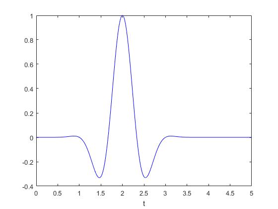
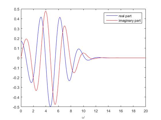
(a) $g(t)$	(b) $\hat{g}(\omega)$

Figure 1: The exact pulse function $g(t)$ and its Fourier transformation $\hat{g}(\omega)$.

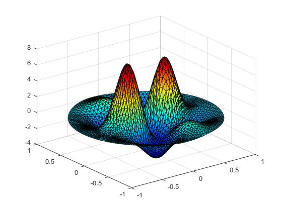
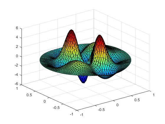
(a) $f_{1}$	(b) $f_{2}$
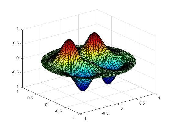
(c) $f_{p}$	(d) $f_{s}$

Figure 2: The exact spatial source function $f=(f_{1},f_{2})$ and its compressional component $f_{p}$ and shear component $f_{s}$.

Below we present several numerical examples to demonstrate the validity and effectiveness of the proposed method. In the following we always choose

$$\hat{g}(\omega)=\int_{0}^{T}\,g(t)\exp(i\omega t)dt,\quad g(t)=\begin{cases}\cos(1.5\pi(t-t_{0}))\exp(-\pi(t-t_{0})^{2}),&t\leq T,\cr 0,&t>T,\end{cases}$$

where $T=5$, $t_{0}=2$. The functions $\hat{g}$ and $g$ are plotted in Figure 1, which shows that $\hat{g}$ is nonzero in $(0,20)$. The source function $f$ in $B_{R}$ with $R=1$ is defined by

$$f=(f_{1},f_{2})^{\top}=\nabla\,f_{p}+\overrightarrow{\mbox{curl}}\,f_{s},$$

where

$$f_{p}(x) = 0.3(1-3x_{1})^{2}\exp(-9x_{1}^{2}-(3x_{2}+1)^{2})-(0.6x_{1}-27x_{1}^{3}-3^{5}x_{2}^{5})\exp(-9x_{1}^{2}-9x_{2}^{2})$$

$$- 0.03\exp(-(3x_{1}+1)^{2}-9x_{2}^{2}),$$

$$f_{s}(x) = 135x_{1}^{2}x_{2}\exp(-9x_{1}^{2}-9x_{2}^{2});$$

see Figure 2. We choose $\mu=1$, $\lambda=2$, $\rho=1$ and $R=2$. The scattering data is collected at 64 uniformly distributed points on the circle $\partial B_{R}$. The total number of iterations is set to be $L=10$.

In the static case, we simulate the data $\hat{U}(x,\omega)$ by solving the inhomogeneous time-harmonic Navier equation using finite element method coupled with an exact transparent boundary condition. Then the compressional and shear parts, $\hat{u}_{p}$ and $\hat{u}_{s}$, are decoupled from $\hat{U}(x,\omega)$ via (5.2)-(5.4). The near-field data of twenty equally spaced frequencies from 1 to 20 are calculated. Figure 3 shows the reconstructed $S_{1}$ and $S_{2}$ from $\{\hat{U}(x,\omega_{k}):|x|=R,k=1,2,\cdots,20\}$, while Figure 4 presents the reconstructed $f_{p}$ and $f_{s}$ from the counterpart of compressional and shear waves, respectively.

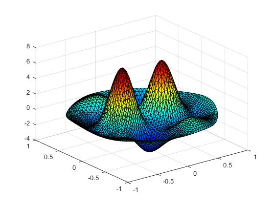
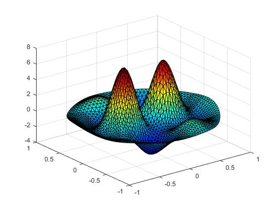
(b) Reconstructed $f_{1}$	(c) Reconstructed $f_{1}$
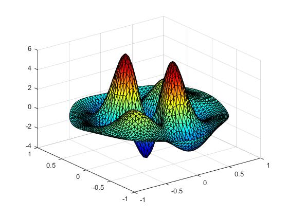
(e) Reconstructed $f_{2}$	(f) Reconstructed $f_{2}$

Figure 3: Reconstructions of $f=(f_{1},f_{2})$ from time-harmonic data at multi frequencies. Figures (b) and (e) are reconstructed from (5.7), whereas (c),(f) are from (5.8).

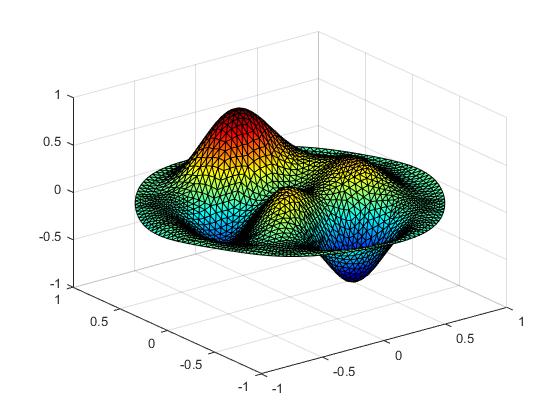
(b) Reconstructed $f_{p}$	(c) Reconstructed $f_{p}$
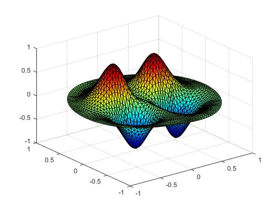
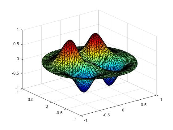
(e) Reconstructed $f_{s}$	(f) Reconstructed $f_{s}$

Figure 4: Reconstructions of the compressional and shear components of $f$. Figures (b) and (e) are reconstructed from (5.9), whereas (c) and (f) are from (5.10).

In the time-dependent case, we first consider the numerical solution of the acoustic wave equation

$$\frac{1}{c_{\alpha}^{2}}\partial_{tt}\,u_{\alpha}(x,t)-\Delta u_{\alpha}(x,t)=g(t)\,f_{\alpha}(x),\;\mbox{in}\quad{\mathbb{R}}^{2}\times{\mathbb{R}}^{+},$$ (5.12)

$$u_{\alpha}|_{t=0}=\partial_{t}u_{\alpha}|_{t=0}=0\quad\mbox{in}\quad{\mathbb{R}}^{2},\quad\alpha=p,s.$$ (5.13)

To reduce the unbounded solution domain to a bounded computational domain, we use the local absorbing boundary condition

$$\partial_{\nu}u_{\alpha}+\frac{1}{c_{\alpha}}\partial_{t}u_{\alpha}+\frac{1}{2R}u_{\alpha}=0\quad\mbox{on}\quad\partial B_{R}.$$

Then the solutions to the acoustic scattering problem (5.12)-(5.13) are computed over $B_{R}$ by using interior penalty discontinuous Galerking method in space and Newmark method in time. Consequently, the data $U(x,t)$ of the Lamé system are obtained through

$$U(x,t)=\frac{1}{\gamma_{p}}\mbox{grad}\,u_{p}(x,t)+\frac{1}{\gamma_{s}}\overrightarrow{\mbox{curl}}\,u_{s}(x,t).$$

In our numerical examples, we collect the scattering data $U(x,t)|_{\partial B_{R_{1}}}$ for $t\in[0,T]$ with $T=20>T_{0}+(R+R_{1})/c_{s}=8$. In Figure 5, we compare the scattering data $\hat{u}(x,\omega)|_{\partial B_{R}}$ at frequencies $\omega=3$ and $\omega=10$ obtained by solving the time-harmonic Lamé system and that by applying Fourier transform (denoted by $\hat{u}^{\prime}(x,\omega)|_{\partial B_{R}}$) to the time-dependent data $U(x,t)|_{\partial B_{R}}$. It can be seen that the data set via Fourier transformation slightly differs from those time-harmonic data, possibly due to numerical errors in the Fourier transform and in the numerical scheme for solving time-dependent Lamé systems as well. To Fourier transform the time domain data, we use fifteen equally spaced frequencies from 1 to 15. Numerical solutions for reconstructing $f$ and $f_{\alpha},\alpha=p,s$ are presented in Figures 6 and 7, respectively. We conclude from Figures 3-7 that satisfactory reconstructions are obtained through the proposed Landweber iterative algorithm.

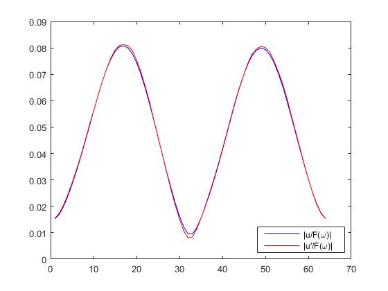
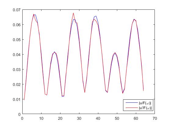
(a) $\omega=3$	(b) $\omega=10$

Figure 5: Comparison of the scattering data $\hat{u}(x,\omega)/\hat{g}(\omega)$ and $\hat{u}^{\prime}(x,\omega)/\hat{g}(\omega)$ at $\omega=3,10$ obtained respectively by solving the time-harmonic Navier equation (blue) and by applying Fourier transform to the time-domain data (red).

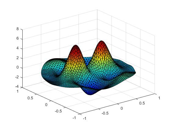
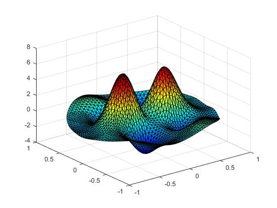
(b) Reconstructed $f_{1}$	(c) Reconstructed $f_{1}$
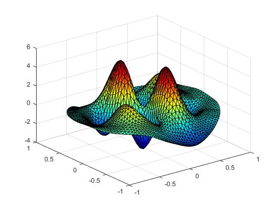
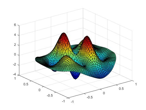
(e) Reconstructed $f_{2}$	(f) Reconstructed $f_{2}$

Figure 6: Reconstructions of $f=(f_{1},f_{2})$ from Fourier-transformed time-domain scattering data. Figures (b) and (e) are reconstructed from (5.7), whereas (c) and (f) are from (5.8).

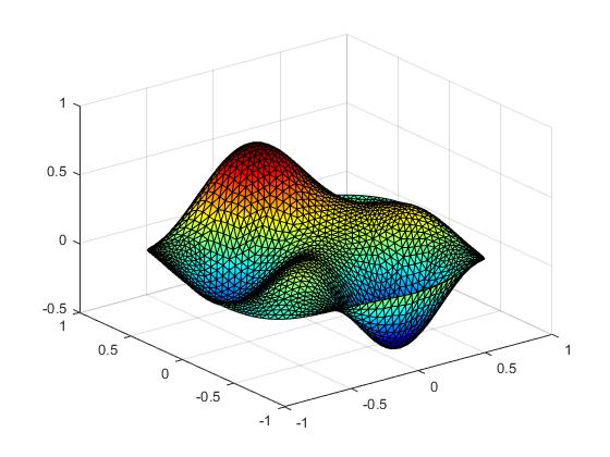
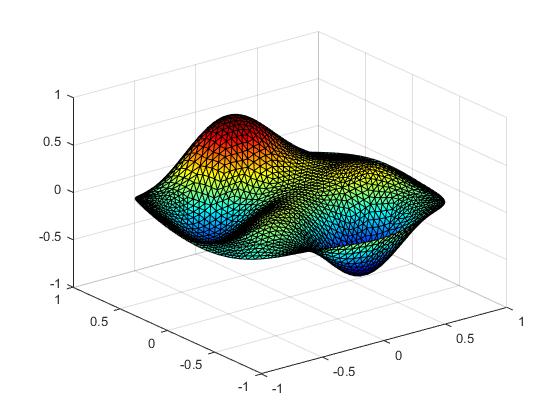
(b) Reconstructed $f_{p}$	(c) Reconstructed $f_{p}$
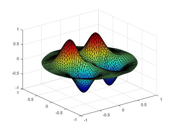
(e) Reconstructed $f_{s}$	(f) Reconstructed $f_{s}$

Figure 7: Reconstructions of the compressional and shear components of $f$ from Fourier-transformed time-domain scattering data. Figures (b) and (e) are reconstructed from (5.9), whereas (c) and (f) are from (5.10).

5.2 Reconstruction of temporal functions

We consider the inverse problem of reconstructing $g$ from the wave fields $\{U(x,t):x\in\Gamma\subset\partial B_{R},t\in(0,T)$ for some $T>0$ in three dimensions. For simplicity we choose the scalar spatial function to be the delta function, i.e., $f(x)=\delta(x)$. Then the function $W$ (see the proof of Theorem 4.4) takes the form

$$W(x,\omega) = \int_{{\mathbb{R}}^{3}}\hat{G}(x-y,\omega)f(y)\,dy$$

$$= \hat{G}(x,\omega)$$

$$= \frac{1}{\mu}\Phi_{k_{s}}(x)\textbf{I}+\frac{1}{\rho\omega^{2}}\,{\rm grad\,}_{x}\,{\rm grad\,}_{x}^{\top}\;\left[\Phi_{k_{s}}(x)-\Phi_{k_{p}}(x)\right],$$

where $\Phi_{k}(x)=e^{ik|x|}/(4\pi|x|)(k=k_{p},k_{s})$. Hence, $f$ is indeed not a non-radiation source for all $\omega\in{\mathbb{R}}^{+}$. In our example, we set the vector temporal function $g(t)$ to be

$$g(t)=(g_{1},g_{2},g_{3})^{\top},$$

$$g_{1}(t)=\begin{cases}\cos(1.5\pi(t-t_{1}))\exp(-\pi(t-t_{1})^{2}),&t\leq T_{1},\cr 0,&t>T_{1},\end{cases}$$

$$g_{2}(t)=\begin{cases}\sin(2\pi(t-t_{2}))\exp(-\pi(t-t_{2})^{2}),&t\leq T_{2},\cr 0,&t>T_{2},\end{cases}$$

$$g_{3}(t)=\begin{cases}\sin(\pi(t-t_{3}))\exp(-\pi(t-t_{3})^{2}),&t\leq T_{3},\cr 0,&t>T_{3},\end{cases}$$

where $T_{1}=5$, $T_{2}=4$, $T_{3}=3$, $t_{1}=2$, $t_{2}=3$ and $t_{3}=2$. The function pairs $(g_{1},\hat{g}_{1})$, $(g_{2},\hat{g}_{2})$ and $(g_{3},\hat{g}_{3})$ are plotted in Figures 1, 8 and 9, respectively. Moreover, we set $g(t)=0$ for $t<0$. With the choice of $f$ and $g$, the forward time-domain scattering data can be expressed as $U=(u_{1},u_{2},u_{3})$, where

$$u_{i}(x,t) = \sum_{j=1}^{3}\int_{0}^{\infty}\int_{{\mathbb{R}}^{3}}G_{i,j}(x-y,t-s)f(y)g_{j}(s)\,dxds$$

$$= \sum_{j=1}^{3}\int_{0}^{\infty}G_{i,j}(x,t-s)g_{j}(s)\,ds$$

$$= \frac{1}{4\pi\rho|x|^{3}}\sum_{j=1}^{3}\left(\frac{x_{i}x_{j}}{c_{p}^{2}}g_{j}(t-|x|/c_{p})+\frac{1}{c_{s}^{2}}(\delta_{ij}|x|^{2}-x_{i}x_{j})g_{j}(t-|x|/c_{s})\right)$$

$$+\frac{1}{4\pi\rho|x|^{3}}\sum_{j=1}^{3}\left(3x_{i}x_{j}-\delta_{ij}|x|^{2}\right)\int_{1/c_{p}}^{1/c_{s}}sg_{j}(t-s)\,ds.$$

Taking the Fourier transform gives the data $\hat{U}(x,\omega_{i})$ in the Fourier domain. The sampling frequencies are chosen as

$$\omega_{j}=1+(j-1)h,\quad h=19/49,\quad j=1,\cdots,K,\quad K=50.$$

Fixing $\omega_{i}\in{\mathbb{R}}^{+}$ ($i=1,2,\cdots,K$), we can always find $x_{0,i}\in\Gamma$ such that $W(x_{0,i},\omega_{i})^{-1}$ exists and the value of the indicator

$$I_{1}(\omega_{i})=[W(x_{0,i},\omega_{i})]^{-1}\hat{U}(x_{0,i},\omega_{i})$$

is identical to $\hat{g}(\omega_{i})$. Taking the inverse Fourier transform of the indicator function $I_{1}(\omega)$ enables us to plot the function $t\rightarrow g_{i}(t)$ ($i=1,2,3$). In our tests we choose $x_{0,i}=(1,1,0)^{\top}$ uniformly in all $i=1,2,\cdots,K$. Numerical reconstructions of $\hat{g}_{i},i=1,2,3$ from the indicator $I_{1}$ are presented in Figure 10.

One can readily observe that the choice of $x_{0,i}$ is not unique. Our numerics show that $\mbox{Det}(W(x,\omega_{i}))$ does not vainish for almost all $x\in\partial B_{R}$. For $\omega_{i}\in{\mathbb{R}}^{+}$, we denote by $\{x_{j,i}:j=1,2,\cdots M\}$ a set of points lying on $|x|=R$ such that $W(x_{j,i},\omega_{i})$ is invertible for each $j$. To make our inversion scheme computationally stable, we can calculate $I_{1}(\omega_{i})$ using each $x_{j,i}$ ($j=1,2,\cdots,M$) and then take the average as the value of $\hat{g}(\omega_{i})$. Hence, we propose another indicator function in the Fourier domain as following

$$I_{2}(\omega_{i}):=\frac{1}{M}\sum_{j=1}^{M}[W(x_{j,i},\omega_{i})]^{-1}\hat{U}(x_{j,i},\omega_{i}),\quad i=1,2,\cdots,K,$$

where the time domain data $\{U(x_{j,i},t):j=1,2,\cdots,M,i=1,2,\cdots,K\}$ are used. In our experiments, we make use of the boundary data equivalently distributed on $|x|=R$ and set

$$x_{j,i}=x_{j}=(\cos((j-1)d\theta),1,\sin((j-1)h))^{\top},\quad h=2\pi/M,j=1,2,\cdots,M,$$

uniformly in all $i=1,2,\cdots,K$. Numerics show that such kind of boundary data are adequate for the choice of $f$ and $g$. Next we consider reconstructions from the noised data

$$U_{\delta}(x,t)=(1+\delta\epsilon(x,t))U(x,t)$$

where $\epsilon(x,t)$ is a function whose value is random between -1 and 1, and the noise level $\delta$ is set to be 30%. We present the reconstructions of $\hat{g}_{j}$ ($j=1,2,3$) based on the indicators $I_{1}$ and $I_{2}$ in Figures 11 and 12, respectively. Reconstructions from the inverse Fourier transform of $I_{j}$ (that is, the temporal function $g(t)$) are illustrated in Figures 13 and 14, where the time-domain data with 30% noise are again used. Comparing Figures 11, 12, 13 and 14, one may conclude that the inversion scheme using $I_{2}$ is indeed more computationally stable than $I_{1}$.

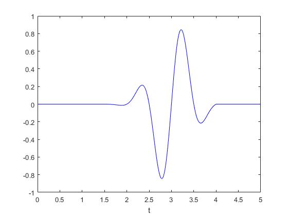
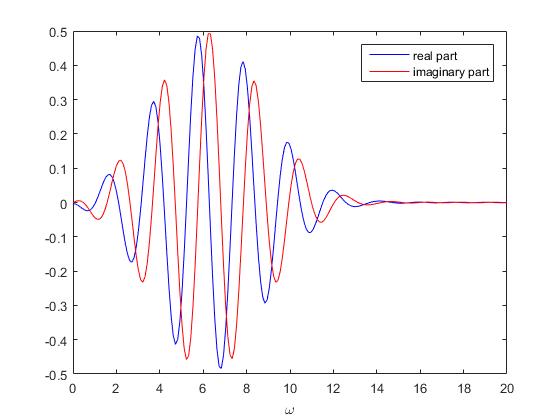
(a) $g_{2}(t)$	(b) $\hat{g}_{2}(\omega)$

Figure 8: The exact pulse function $g_{2}(t)$ and its Fourier transformation $\hat{g}_{2}(\omega)$.

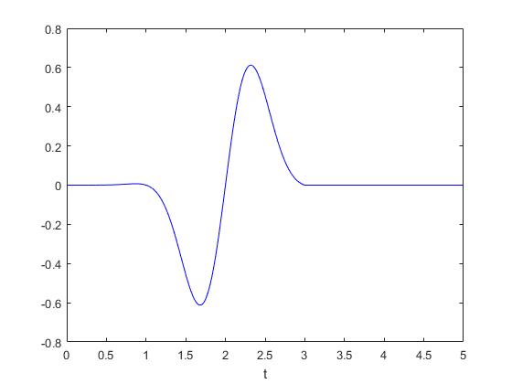
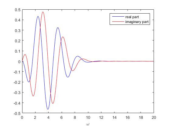
(a) $g_{2}(t)$	(b) $\hat{g}_{2}(\omega)$

Figure 9: The exact pulse function $g_{3}(t)$ and its Fourier transformation $\hat{g}_{3}(\omega)$.

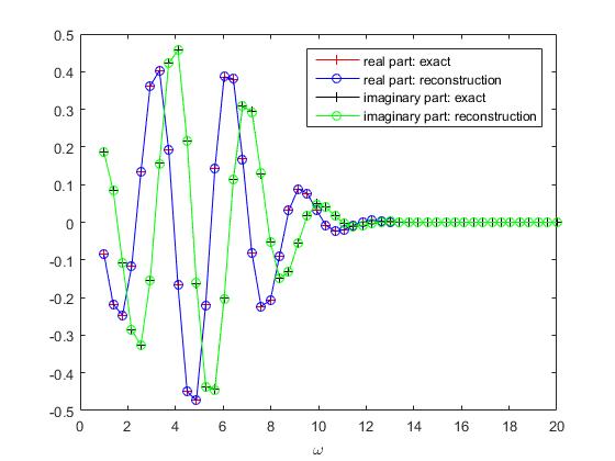
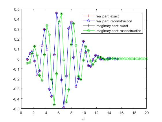
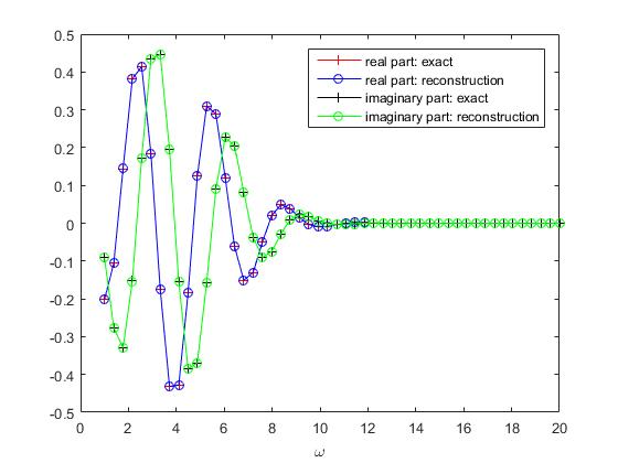
(a) $\hat{g}_{1}$	(a) $\hat{g}_{2}$	(a) $\hat{g}_{3}$

Figure 10: Reconstruction of temporal functions from $I_{1}$ without noise.

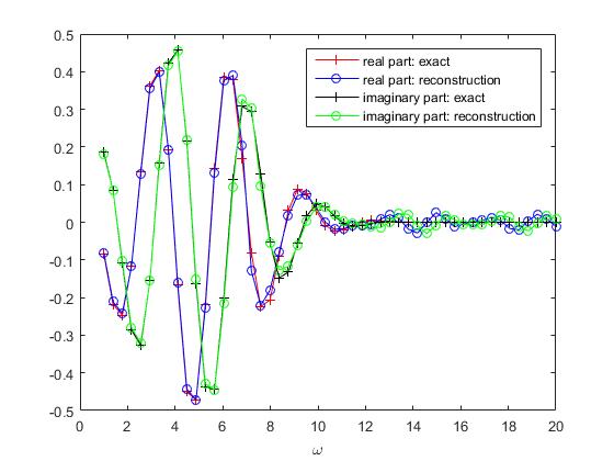
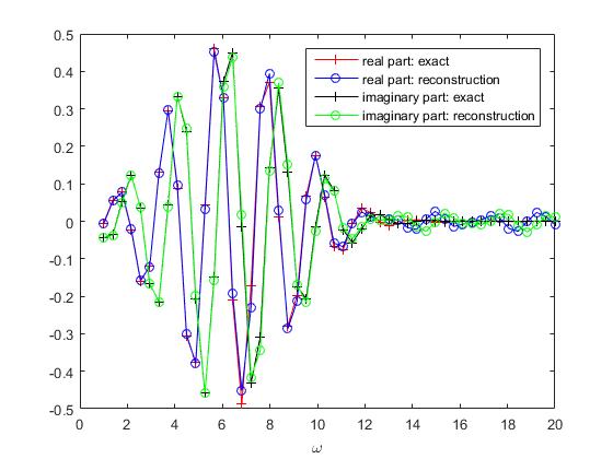
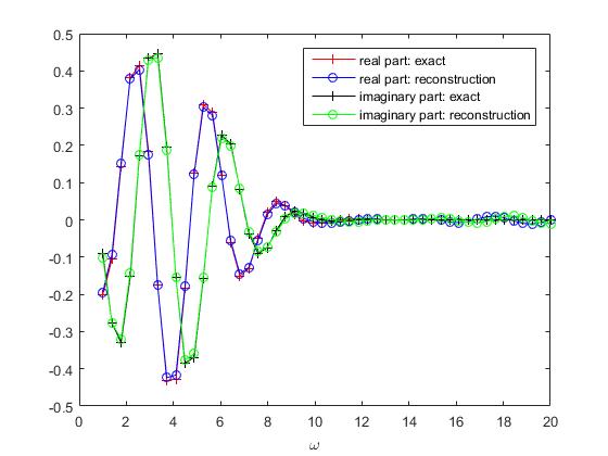
(a) $\hat{g}_{1}$	(a) $\hat{g}_{2}$	(a) $\hat{g}_{3}$

Figure 11: Reconstruction of temporal functions from $I_{1}$ with 30% noise.

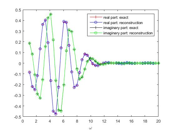
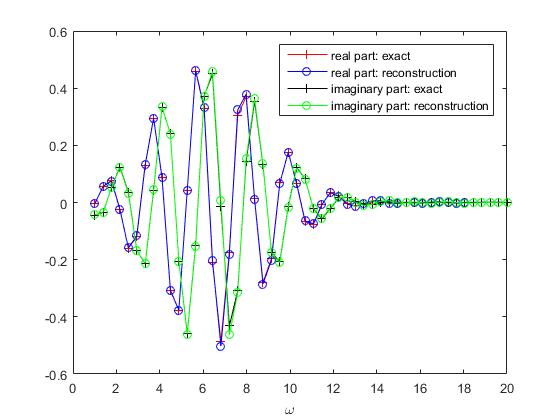
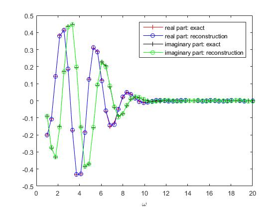
(a) $\hat{g}_{1}$	(a) $\hat{g}_{2}$	(a) $\hat{g}_{3}$

Figure 12: Reconstruction of temporal functions from $I_{2}$ with 30% noise.

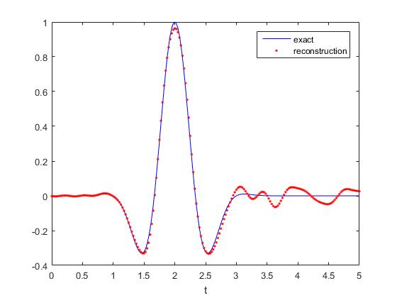
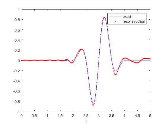
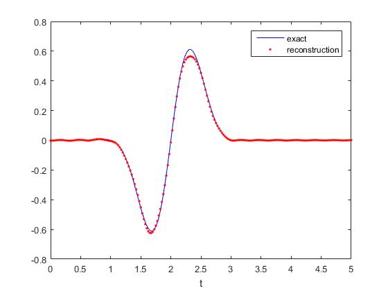
(a) $g_{1}$	(a) $g_{2}$	(a) $g_{3}$

Figure 13: Reconstruction of temporal functions from $\tilde{I}_{1}$ with 30% noise.

(a) $g_{1}$	(a) $g_{2}$	(a) $g_{3}$

Figure 14: Reconstruction of temporal functions from $\tilde{I}_{2}$ with 30% noise.

6 Appendix

Lemma 6.1.

Suppose that $S\in(L^{2}({\mathbb{R}}^{3}))^{3}$ has a compact support in $B_{R}$ for some $R>0$, then the Helmholtz decomposition of $S$ is unique.

Proof.

Due to the Helmholtz decomposition, every $S\in(L^{2}({\mathbb{R}}^{3}))^{3}$ admits a decomposition:

$$S=\nabla\,S_{p}+\nabla\times\,S_{s},\quad\nabla\cdot S_{s}=0,$$

where

$$S_{p}\in H^{1}(B_{R}),\quad S_{s}\in H_{{\rm curl\,}}(B_{R}):=\{U:U\in L^{2}(B_{R})^{3},{\rm curl\,}U\in L^{2}(B_{R})^{3}\}$$

also have compact support in $B_{R}$. Suppose that $S$ admits another orthogonal decomposition $S=\nabla\,S_{p}^{\prime}+\nabla\times\,S_{s}^{\prime},\nabla\cdot S_{s}^{\prime}=0$. Then we have

$$\nabla\,(S_{p}-S_{p}^{\prime})+\nabla\times\,(S_{s}-S_{s}^{\prime})=0.$$ (6.1)

Taking the divergence of both sides of (6.1) gives $\Delta(S_{p}-S_{p}^{\prime})=0$ in $B_{R}$, i.e., $S_{p}-S_{p}^{\prime}$ is harmonic over $B_{R}$. Note that $S_{p}-S_{p}^{\prime}=0$ on $\partial B_{R}$. Applying the maximum principle for harmonic functions yields $S_{p}=S_{p}^{\prime}$ in $B_{R}$. On the other hand, applying $\nabla\times$ to the both sides of (6.1) we obtain

$$0=\nabla\times(\nabla\times\;(S_{s}-S_{s}^{\prime}))=\nabla(\nabla\cdot\,(S_{s}-S_{s}^{\prime}))-\Delta\,(S_{s}-S_{s}^{\prime})=-\Delta\,(S_{s}-S_{s}^{\prime}).$$

Then the relation $S_{s}=S_{s}^{\prime}$ in $B_{R}$ can be proved analogously. This completes the proof. ∎

In the following lemma, the notation $\textbf{I}_{n\times n}$ denotes the unit matrix in ${\mathbb{R}}^{n\times n}$ for $n\geq 2$.

Lemma 6.2.

Let $\xi=(\xi_{1},\cdots,\xi_{n})^{\top}\in{\mathbb{R}}^{n\times 1}$ and $A(\xi)=\mu|\xi|^{2}\textbf{I}_{n\times n}+(\lambda+\mu)\xi\otimes\xi\in{\mathbb{R}}^{n\times n}$. Then the eigenvalues $\tau_{j}$ ($j=1,2,\cdots,n$) of $A(\xi)$ are given by

$$\tau_{1}=(\lambda+2\mu)|\xi|^{2},\quad\tau_{2}=\cdots=\tau_{n}=\mu\,|\xi|^{2}.$$

Proof.

Set $\tilde{A}=A-\tau\textbf{I}_{n\times n}$. We may rewrite $\tilde{A}$ in the form $\tilde{A}=B+VV^{\top}$, where

$$B=(\mu|\xi|^{2}-\tau)\,\textbf{I}_{n\times n},\quad V=\sqrt{\lambda+\mu}\,\xi.$$

Straightforward calculations show that

$$\mbox{Det}(\tilde{A}) = \mbox{Det}(B+VV^{\top})$$

$$= (1+V^{\top}\,B^{-1}\,V)\,\mbox{Det}(B)$$

$$= \left(1+\frac{(\lambda+\mu)|\xi|^{2}}{\mu|\xi|^{2}-\tau}\right)\,(\mu|\xi|^{2}-\tau)^{n}$$

$$= [(\lambda+2\mu)|\xi|^{2}-\tau](\mu|\xi|^{2}-\tau)^{n-1},$$

which implies the eigenvalues of $A$. ∎

Lemma 6.3.

(Grownwall-type inequality) Let $T>0$ and $u\in L^{2}(0,T)$ be nonnegative and fulfill, for almost every $t\in(0,T)$, the inequality

$$u(t)\leq a(t)+\int_{0}^{t}b(s)\,u(s)\,ds,$$ (6.2)

where $a\in L^{2}(0,T)$ and $b\in\mathcal{C}([0,T])$ are two nonnegative functions. Then, for almost every $t\in(0,T)$, we have

$$u(t)\leq a(t)+\int_{0}^{t}a(s)b(s)e^{\int_{s}^{t}b(\tau)d\tau}ds.$$ (6.3)

Proof.

We consider $Y$ defined, for almost every $t\in(0,T)$, by

$$Y(t):=e^{-\int_{0}^{t}b(s)ds}\int_{0}^{t}b(s)u(s)ds$$

and we remark that $Y\in H^{1}(0,T)$ and satisfies $Y(0)=0$. Then, for almost every $t\in(0,T)$, we find

$$Y^{\prime}(t)=b(t)u(t)e^{-\int_{0}^{t}b(s)ds}-b(t)e^{-\int_{0}^{t}b(s)ds}\int_{0}^{t}b(s)u(s)ds.$$

On the other hand, in view of (6.2), for almost every $t\in(0,T)$, we get

$$\int_{0}^{t}b(s)u(s)ds\geq u(t)-a(t)$$

and we deduce that

$$Y^{\prime}(t)\leq a(t)b(t)e^{-\int_{0}^{t}b(s)ds}.$$

Integrating on both side of this inequality we get

$$\int_{0}^{t}Y^{\prime}(s)ds\leq\int_{0}^{t}a(s)b(s)e^{-\int_{0}^{s}b(\tau)d\tau}ds,\quad t\in(0,T).$$

On the other hand, since $Y\in H^{1}(0,T)$ and satisfies $Y(0)=0$, by density one can check that $Y(t)=\int_{0}^{t}Y^{\prime}(s)ds$ which implies that

$$e^{-\int_{0}^{t}b(s)ds}\int_{0}^{t}b(s)u(s)ds\leq\int_{0}^{t}a(s)b(s)e^{-\int_{0}^{s}b(\tau)d\tau}ds$$

and by the same way, for almost every $t\in(0,T)$, the following inequality

$$\int_{0}^{t}b(s)u(s)ds\leq e^{\int_{0}^{t}b(s)ds}\left(\int_{0}^{t}a(s)b(s)e^{-\int_{0}^{s}b(\tau)d\tau}ds\right)=\int_{0}^{t}a(s)b(s)e^{\int_{s}^{t}b(\tau)d\tau}ds.$$

Finally, applying again (6.2), for almost every $t\in(0,T)$, we find

$$u(t)\leq a(t)+\int_{0}^{t}b(s)u(s)ds\leq a(t)+\int_{0}^{t}a(s)b(s)e^{\int_{s}^{t}b(\tau)d\tau}ds.$$

This proves (6.3).∎

References

• [1] J. D. Achenbach, Wave Propagation in Elastic Solids, North-Holland Publishing Company: Amsterdam, 1973.
• [2] K. Aki and P. G. Richards, Quantitative Seismology, 2ed edition, University Science Books, Mill Valley: California, 2002.
• [3] C. Alves, N. Martins and N. Roberty, Full identification of acoustic sources with multiple frequencies and boundary measurements, Inverse Problems Imaging, 3 (2009): 275-294.
• [4] H. Ammari, E. Bretin, J. Garnier and A. Wahab, Time reversal algorithms in viscoelastic media, European J. Appl. Math., 24 (2013): 565-600.
• [5] H. Ammari, E. Bretin, J. Garnier, H. Kang, H. Lee and A. Wahab, Mathematical Methods in Elasticity Imaging, Princeton University Press: Princeton, 2015.
• [6] Y. Kian, D. Sambou, E. Soccorsi, Logarithmic stability inequality in an inverse source problem for the heat equation on a waveguide, arXiv:1612.07942, 2016.
• [7] Yu. E. Anikonov, J. Cheng and M. Yamamoto, A uniqueness result in an inverse hyperbolic problem with analyticity, European Journal of Applied Mathematics, (15) 2004: 533-543.
• [8] G. Bao, G. Hu, J. Sun and T. Yin, Direct and inverse elastic scattering from anistropic media, arXiv:1612.06604, 2016.
• [9] G. Bao, J. Lin and F. Triki, A multi-frequency inverse source problem, J. Differ. Equ., 249 (2010): 3443-3465.
• [10] G. Bao, S. Lu, W. Rundell and B. Xu, A recursive algorithm for multi-frequency acoustic inverse source problems, SIAM J. Numer. Anal., (53) 2015: 1608-1628.
• [11] G. Bao, P. Li, J. Lin and F. Triki, Inverse scattering problems with multi-frquencies, Inverse Problems, 31 (2015): 093001.
• [12] M. Bonnet and A. Constantinescu, Inverse problems in elasticity, Inverser Problems 21 (2005): R1-R50.
• [13] A.L. Bukhgeim and M.V. Klibanov, Global uniqueness of a class of multidimensional inverse problems, Sov. Math., Dokl., 24 (1981): 244-247.
• [14] M. Costabel, Time-dependent problems with the boundary integral equation method, Encyclopedia of Computational Mechanics (2004): 1-25.
• [15] M. Choulli and M. Yamamoto, Some stability estimates in determining sources and coefficients, J. Inverse Ill-Posed Probl., 14 (2006): 355-373.
• [16] M. Eller and N. Valdivia, Acoustic source identification using multiple frequency information, Inverse Problems, 25 (2009): 115005.
• [17] K. Fujishiro and Y. Kian, Determination of time dependent factors of coefficients in fractional diffusion equations, Math. Control Relat. Fields, 6 (2016): 251-269.
• [18] O.Y. Imanuvilov and M. Yamamoto, Global Lipschitz stability in an inverse hyperbolic problem by interior observations, Inverse Probl., 17 (2001): 717-728.
• [19] O.Y. Imanuvilov and M. Yamamoto, Global uniqueness and stability in determining coefficients of wave equations, Comm. Partial Differential Equations, 26 (2001): 1409-1425.
• [20] V. Isakov, Carleman type estimates in an anisotropic case and applications, Journal of Differential Equations, 105 (1993): 217-238.
• [21] V. Isakov, Inverse Problems for Partial Differential Equations, Springer-Verlag: Berlin, 1998.
• [22] D. Jiang, Y. Liu and M. Yamamoto, Inverse source problem for the hyperbolic equation with a time-dependent principal part, J. Differential Equations, 262 (2017): 653-681.
• [23] Y. Kian, D. Sambou, E. Soccorsi, Logarithmic stability inequality in an inverse source problem for the heat equation on a waveguide, arXiv:1612.07942, 2016.
• [24] A. Khaǐdarov, Carleman estimates and inverse problems for second order hyperbolic equations, Math. USSR Sbornik, 58 (1987): 267-277.
• [25] M. V. Klibanov, Inverse problems and Carleman estimates, Inverse Problems, 8 (1992): 575-596.
• [26] R. Leis, Initial Boundary Value Problems in Mathematical Physics, Wiley: New York, 1986. .
• [27] J. L. Lions and E. Magenes, Non-homogeneous Boundary Value Problems and Applications, Vol. I and II (English translation), Springer-Verlag: Berlin, 1972.
• [28] M. Mabrouk and Z. Helali, The scattering theory of C. Wilcox in elasticity, Math. Meth. Appl. Sci., (25) 2002: 997-1044.
• [29] Rakesh and W. W. Symes, Uniqueness for an inverse problem for the wave equation, Comm. in Partial Differential Equations, 13 (1988): 87-96.
• [30] L. Robbiano and C. Zuily, Uniqueness in the Cauchy problem for operators with partially holomorphic coefficients, Invent. Math., 131 (1998), 493-539.
• [31] D. Tataru, Carleman estimates and unique continuation for solutions to boundary value problems, J. Math. Pure Appl., 75 (1996): 367-408.
• [32] M. Yamamoto, Stability, reconstruction formula and regularization for an inverse source hyperbolic problem by control method, Inverse Problems, (11) 1995: 481-496.
• [33] M. Yamamoto, Uniqueness and stability in multidimensional hyperbolic inverse problems, J. Math. Pure Appl., 78 (1999): 65-98.