Finite Element Lattice Boltzmann Simulations of Contact Line Dynamics

Abstract

The lattice Boltzmann method has become a standard technique for simulating a wide range of fluid flows. However, the intrinsic coupling of momentum and space discretization restricts the traditional lattice Boltzmann method to regular lattices. Alternative off-lattice Boltzmann schemes exist for both single- and multiphase flows that decouple the velocity discretization from the underlying spatial grid. The current study extends the applicability of these off-lattice methods by introducing a finite element formulation that enables simulating contact line dynamics for partially wetting fluids. This work exemplifies the implementation of the scheme and furthermore presents benchmark experiments that show the scheme reduces spurious currents at the liquid-vapor interface by two orders of magnitude compared to a nodal implementation and allows for predicting the equilibrium states accurately in the range of moderate contact angles.

I Introduction

The interaction between a liquid and a solid surface plays an important role in many fields ranging in scale from below those considered in microfluidics to scales beyond those in reservoir modelling. In this context the static contact angle defines the intersection between a liquid-vapor interface and a solid surface and specifies the degree of wettability of the surface through Young’s equation.

The lattice Boltzmann method (LBM) is a popular method within computational fluid dynamics and several regular-grid based multiphase formulations have emerged within the last 15 years that succesfully describe fluid-solid interactions, thereby enabling the simulation of wetting effects. These formulations fall within different categories such as free-energy (Briant (2002); Briant et al. (2004); Briant and Yeomans (2004); Lee and Liu (2008); Liu and Lee (2009); Lee and Liu (2010); Connington and Lee (2013)) and interparticle-potential (Huang et al. (2007); Schmieschek and Harting (2011); Jansen et al. (2013)) schemes and have been used, for example, in studies of droplet spreading (e.g. Jansen et al. (2013); Connington and Lee (2013); Son et al. (2015); Wang et al. (2013)) and fluid flow in porous media (e.g. Liu et al. (2013); Ghassemi and Pak (2011); Yiotis et al. (2007); Langaas and Papatzacos (2001); Huang and yun Lu (2009); Huang et al. (2009); Liu et al. (2015)). In particular free-energy based LBMs have become a useful tool for the study of wetting phenomena Huang et al. (2015). One of the main advantages of these models over other variants such as interparticle potential (Shan-Chen) is that the surface tension is more easily tuned and the kinematic viscosity ratio and density ratio can be chosen independently Huang et al. (2015). Free-energy based LBMs enforce the wetting boundary condition on the wall implicitly in the intermolecular force. On regular grids this is accomplished by specifying the terms in the finite-difference derivatives at the solid boundary Liu and Lee (2009); Lee and Liu (2010); Connington and Lee (2013); Connington et al. (2015).

A different class of LBM exists generally known as off-lattice Boltzmann methods, where the spatial and temporal discretizations are decoupled for enhanced geometric flexibility. This class consists of finite volume Rossi et al. (2005); Patil and Lakshmisha (2009); Misztal et al. (2015a) and finite element schemes Lee and Lin (2001, 2003); Bardow et al. (2006); Misztal et al. (2015b); Wardle and Lee (2013); Matin et al. (2017). However, previous work on multiphase finite element LBM (FE-LBM) has only regarded the intermolecular force term Wardle and Lee (2013); Matin et al. (2017) and liquid-solid interactions have not been accounted for. In this paper we present an extension of our previous characteristic-based FE-LBM scheme Matin et al. (2017) by implementing wetting boundary conditions and moving the intermolecular force term to the streaming step. Our formulation is shown to further reduce spurious currents at equilibrium compared to the implementation in Matin et al. (2017). To the best of our knowledge, this is the first formulation of wetting boundaries in the framework of off-lattice Boltzmann methods.

The paper is organized as follows: In Section II the multiphase model and wall boundary conditions are briefly reviewed. This section also details the FE-LBM on unstructured grids. The scheme is validated in Section III and results are summarized in Section IV.

II Numerical Method

We consider the diffuse interface model for incompressible immiscible two-phase flows with large density and kinematic viscosity ratios presented in Lee and Liu (2010); Wardle and Lee (2013); Connington and Lee (2013). The main aspects of the model are briefly summarized in the following to provide context.

The composition $C\in[0,1]$ is chosen as the volume fraction of the liquid phase, i.e., $C=1$ for the liquid ($l$) phase and $C=0$ for the vapor ($v$) phase. The time evolution of the diffuse interface is governed by a Cahn-Hilliard equation

$$\partial_{t}C+\mathbf{u}\cdot\nabla C=M\nabla^{2}\mu,$$ (1)

where $M>0$ is the mobility. The chemical potential $\mu$ in Eq. (1) follows from the free-energy functional

$$\Psi_{b}=\int_{V}{\bigg{(}\beta C^{2}(1-C)^{2}+\frac{\kappa}{2}|\nabla C|^{2}\bigg{)}dV},$$ (2)

where $E_{0}(C)=\beta C^{2}(1-C)^{2}$ is the bulk free energy density. Here $\beta$ and $\kappa$ are constants related to the surface tension and interface width. From thermodynamics it follows that

$$\mu=\frac{\delta\Psi_{b}}{\delta C}=2\beta C(C-1)(2C-1)-\kappa\nabla^{2}C$$ (3)

and the plane interfacial profile in equilibrium follows from setting $\mu=0$,

$$C(z)=\frac{1}{2}+\frac{1}{2}\tanh\!\bigg{(}\frac{2z}{\xi}\bigg{)}.$$ (4)

Here $z$ is the coordinate normal to the interface, $\xi=\sqrt{8\kappa/\beta}$ the interface thickness and $\sigma=\sqrt{2\kappa\beta}/6$ its surface tension. Disregarding body forces, the governing macroscopic equations for the incompressible flow are

$$\nabla\cdot\mathbf{u} =0$$ (5)

$$\rho\bigg{(}\!\partial_{t}\mathbf{u}+\mathbf{u}\cdot\nabla\mathbf{u}\bigg{)} =-\nabla p-C\nabla\mu$$ (6)

$$\phantom{{}=}+\nabla\cdot[\eta(\nabla\mathbf{u}+(\nabla\mathbf{u})^{T})]$$

where $p$ is the hydrodynamic pressure, $\eta$ the dynamic viscosity and $\rho=C\rho_{l}+(1-C)\rho_{v}$ the density.

II.1 Lattice Boltzmann Method

Recovering the Cahn-Hilliard, pressure evolution and momentum equations in a lattice Boltzmann framework can be accomplished by introducing two particle distribution functions $g_{\alpha}$ and $h_{\alpha}$. The distribution function $h_{\alpha}$ recovers the composition that tracks the interface between the two phases and $g_{\alpha}$ recovers the hydrodynamic flow fields. The lattice Boltzmann equation for each distribution function is given by Lee and Liu (2010); Wardle and Lee (2013)

$$\partial_{t}g_{\alpha}+e_{\alpha i}\partial_{i}g_{\alpha} =-\Omega_{g_{\alpha}}+F_{g_{\alpha}}$$ (7)

$$\partial_{t}h_{\alpha}+e_{\alpha i}\partial_{i}h_{\alpha} =-\Omega_{h_{\alpha}}+F_{h_{\alpha}}$$ (8)

where the intermolecular forcing term $F_{\psi_{\alpha}}$ and BGK-operator $\Omega_{\psi_{\alpha}}$ for a given distribution function $\psi\in\{g,h\}$ is

$$\Omega_{\psi_{\alpha}}= +\frac{1}{\lambda}(\psi_{\alpha}-\psi_{\alpha}^{\text{eq}})$$ (9)

$$F_{g_{\alpha}}= +(e_{\alpha i}-u_{i})\Big{[}\partial_{i}\rho c_{s}^{2}(\Gamma_{\alpha}(\mathbf{u})-\Gamma_{\alpha}(0))$$ (10)

$$+\mu(\partial_{i}C)\Gamma_{\alpha}(\mathbf{u})\Big{]}$$

$$F_{h_{\alpha}}= +(e_{\alpha i}-u_{i})\bigg{[}\partial_{i}C-\frac{C}{\rho c_{s}^{2}}(\partial_{i}p-\mu\partial_{i}C)\bigg{]}\Gamma_{\alpha}(\mathbf{u})$$ (11)

$$+M(\partial_{k}\partial_{k}\mu)\Gamma_{\alpha}(\mathbf{u})$$

Here $e_{\alpha i}$ denote the discrete particle velocities in directions $\alpha$ of the velocity lattice and the current work employs the D3Q19 lattice. The relaxation parameter $\lambda$ is proportional to the kinematic viscosity $\nu$, $\nu=\eta/\rho=c_{s}^{2}\lambda=c_{s}^{2}\tau\delta t$, where we use the definition $\tau\equiv\lambda/\delta t$. It is taken as the harmonic mean of the bulk relaxation parameters $(\tau_{l},\tau_{v})$ weighted by $C$ Lee and Liu (2010),

$$\frac{1}{\tau}=\frac{C}{\tau_{l}}+\frac{1-C}{\tau_{v}}.$$ (12)

The equilibrium distribution functions $g_{\alpha}^{\text{eq}}$ and $h_{\alpha}^{\text{eq}}$ of Eqs. (7)-(8) are

$$g_{\alpha}^{\text{eq}} =w_{\alpha}\bigg{[}p+\rho c_{s}^{2}\bigg{(}\frac{e_{\alpha i}u_{i}}{c_{s}^{2}}+\frac{(e_{\alpha i}e_{\alpha j}-c_{s}^{2}\delta_{ij})u_{i}u_{j}}{2c_{s}^{4}}\bigg{)}\bigg{]}$$ (13)

$$h_{\alpha}^{\text{eq}} =w_{\alpha}C\bigg{[}1+\frac{e_{\alpha i}u_{i}}{c_{s}^{2}}+\frac{(e_{\alpha i}e_{\alpha j}-c_{s}^{2}\delta_{ij})u_{i}u_{j}}{2c_{s}^{4}}\bigg{]}$$ (14)

$$\equiv\Gamma_{\alpha}(\mathbf{u})C$$ (15)

where $w_{\alpha}$ are the integral weighting factors of the D3Q19 model. Using the Chapman-Enskog expansion, Eqs. (7)-(8) can be shown to recover Eqs. (1) and (5)-(6) to second-order accuracy at low Mach numbers. The hydrodynamic fields are calculated by taking the zeroth and the first moments of the distribution functions Lee and Liu (2010)

$$C =\sum_{\alpha}h_{\alpha}$$ (16)

$$\rho u_{i} =\frac{1}{c_{s}^{2}}\sum_{\alpha}e_{\alpha i}g_{\alpha}$$ (17)

$$p =\sum_{\alpha}g_{\alpha}$$ (18)

II.2 Boundary Conditions

Incorporating contact angles can be accomplished by adding to the free energy functional $\Psi_{b}$ a surface term $\Psi_{s}$ which accounts for the interaction between the liquid-vapor interface and solid surface. Expanded as a power series in the composition calculated at the solid surface, $C_{s}$, the surface term takes the form de Gennes (1985)

$$\Psi_{s}=\int_{S}{\big{(}\phi_{0}-\phi_{1}C_{s}+\phi_{2}C_{s}^{2}-\phi_{3}C_{s}^{3}\big{)}dS},$$ (19)

where terms up to cubic order are retained. The constants $\phi_{i}$ for $i\in\{1,2,3\}$ are given by $\phi_{0}=\phi_{1}=0$, $\phi_{2}=\phi_{c}/2$ and $\phi_{3}=\phi_{c}/3$, where $\phi_{c}$ is a constant that recovers the desired contact angle Liu and Lee (2009); Lee and Liu (2010); Connington and Lee (2013). In the linear and quadratic approximations the liquid phase at the solid surface is enriched relative to the bulk value by the attraction on wetting surfaces and depleted due to the repulsion on non-wetting surfaces Liu and Lee (2009). This effect is undesirable in the systems that the current work is directed towards, and the cubic approximation is thus utilized which displays equilibrium densities at the solid surface that are equal to the corresponding bulk values.

The first boundary condition required for Eq. (1) ensures no mass flux normal to a solid boundary due to a chemical potential gradient Lee and Liu (2010); Connington and Lee (2013),

$$\mathbf{n}\cdot\nabla\mu|_{S}=0,$$ (20)

and is satisfied when bounce-back is employed at the solid boundary. The second boundary condition is for $\nabla^{2}C$ and can be established by minimizing $\Psi_{s}$ Liu and Lee (2009),

$$\mathbf{n}\cdot\nabla C|_{S}=\frac{\phi_{c}}{\kappa}(C_{s}-C_{s}^{2}),$$ (21)

where the equilibrium contact angle $\theta_{\text{eq}}$ follows from Young’s equation for a given wetting potential $\Omega_{c}$ $\cos\theta_{\text{eq}}=-\Omega_{c}=-\phi_{c}/\sqrt{2\kappa\beta}$. Alternative formulations of this boundary condition exist such as the geometric formulation presented in Ding and Spelt (2007).

Simulating wetting effects with the lattice Boltzmann method thus reduces to implicitly imposing Eq. (21) at the solid boundary in the relevant terms of the intermolecular forces. On regular grids this is accomplished by specifying the terms in the finite-difference derivatives at the solid boundary, see e.g., Liu and Lee (2009); Lee and Liu (2010); Connington and Lee (2013); Connington et al. (2015). In the following we describe a method for enforcing them on an irregular grid.

II.3 Finite Element Method

Equations (7)-(8) can be solved at any point by streaming along characteristics from $(\mathbf{x},t)$ to $(\mathbf{x}+\delta t\mathbf{e}_{\alpha},t+\delta t)$ (where $\delta t$ is the time step), and applying the trapezoid rule to the RHS Lee and Lin (2003); Connington et al. (2015); Matin et al. (2017).

$$\psi_{\alpha}(\mathbf{x}+\delta t\mathbf{e}_{\alpha},t+\delta t)-\psi_{\alpha}(\mathbf{x},t)=$$ (22)

$$\frac{\delta t}{2}(F_{\psi_{\alpha}}-\Omega_{\psi_{\alpha}})|_{(\mathbf{x},t)}+\frac{\delta t}{2}(F_{\psi_{\alpha}}-\Omega_{\psi_{\alpha}})|_{(\mathbf{x}+\delta t\mathbf{e}_{\alpha},t+\delta t)}.$$

By introducing the new variable $\bar{\psi}_{\alpha}(\mathbf{x},t)=\psi_{\alpha}+\frac{\delta t}{2}\Omega_{\psi_{\alpha}}$ we can recast Eq. (22) as

$$\bar{\psi}_{\alpha}(\mathbf{x}+\delta t\mathbf{e}_{\alpha},t+\delta t)-\bar{\psi}_{\alpha}(\mathbf{x},t)=$$ (23)

$$-\frac{1}{\tau+0.5}(\bar{\psi}_{\alpha}-\bar{\psi}_{\alpha}^{\text{eq}})+\frac{\delta t}{2}\left(F_{{\psi}_{\alpha}}|_{(\mathbf{x},t)}+F_{\psi_{\alpha}}|_{(\mathbf{x}+\delta t\mathbf{e}_{\alpha},t+\delta t)}\right)$$

where $\bar{\psi}^{\text{eq}}_{\alpha}=\psi^{\text{eq}}_{\alpha}$, $\tau=\lambda/{\delta t}$, and the moments of $\bar{\psi}$ recover the same macroscopic fields as the moments of $\psi$. The force term can be treated in an implicit manner and integrated locally in the collision step Matin et al. (2017). It is observed, however, that integrating the force term in the streaming step as done in Wardle and Lee (2013) greatly enhances stability when simulating surface wettability, and allows to minimize spurious currents through careful selection of the spatial discretization scheme (as discussed in greater detail below).

Equation (23) is solved at a grid point $\mathbf{x}_{i}$ using the standard two-step procedure:

Collision

$$\hat{\psi}_{\alpha}^{n}=\bar{\psi}_{\alpha}^{n}-\frac{1}{\tau+0.5}\left(\bar{\psi}_{\alpha}^{n}-\bar{\psi}_{\alpha}^{\text{eq},n}\right)$$ (24)

Streaming

$$\bar{\psi}_{\alpha}^{n+1} =\hat{\psi}_{\alpha}^{n}-\delta t\big{(}e_{\alpha i}\partial_{i}\hat{\psi}_{\alpha}^{n}-F^{n}_{\psi_{\alpha}}\big{)}$$ (25)

$$\phantom{{}=f_{\alpha}^{n}}+\frac{\delta t^{2}}{2}e_{\alpha j}\partial_{j}\big{(}e_{\alpha i}\partial_{i}\hat{\psi}_{\alpha}^{n}-F^{n}_{\psi_{\alpha}}\big{)}$$

where the superscripts correspond to the time step. Equation (25) is obtained from (23) by approximating

$$\hat{\psi}^{n}(\mathbf{x}_{i}-\delta t\mathbf{e}_{\alpha}) =\hat{\psi}^{n}(\mathbf{x}_{i})-\delta te_{\alpha i}\partial_{i}\hat{\psi}_{\alpha}^{n}$$ (26)

$$\phantom{{}=\hat{\psi}^{n}(\mathbf{x}_{i})}+\frac{\delta t^{2}}{2}e_{\alpha j}e_{\alpha_{i}}\partial_{j}\partial_{i}\hat{\psi}_{\alpha}^{n}+\mathcal{O}(\delta t^{3}),$$

$$F^{n}_{\psi_{\alpha}}(\mathbf{x}_{i}-\delta t\mathbf{e}_{\alpha}) =F^{n}_{\psi_{\alpha}}(\mathbf{x}_{i})-\delta te_{\alpha i}\partial_{i}F^{n}_{\psi_{\alpha}}+\mathcal{O}(\delta t^{2}),$$ (27)

$$F^{n+1}_{\psi_{\alpha}}(\mathbf{x}_{i}) =F^{n}_{\psi_{\alpha}}(\mathbf{x}_{i})+\mathcal{O}(\delta t).$$ (28)

We note that $F^{n+1}_{\psi_{\alpha}}(\mathbf{x}_{i})$ is approximated by $F^{n}_{\psi_{\alpha}}(\mathbf{x}_{i})$ in order to avoid implicitness. This approximation still yields a second-order accurate and conditionally stable expression in time (see appendix of Lee et al. (2006)). Intuitively, the approximation follows from the observation that the macroscopic fields recovered by $\tilde{\psi}_{\alpha}$ change at a much slower rate than the individual populations.

Equation (25) is discretized in space using the Galerkin finite element method, where spatial decomposition using linear, tetrahedral elements has been applied. The particle distribution functions are specified at the mesh nodes (vertices) $\mathbf{x}_{1},\mathbf{x}_{2},\ldots,\mathbf{x}_{N_{V}}$ and interpolated at other points,

$$\bar{\psi}_{\alpha}(\mathbf{x})\approx\tilde{\psi}_{\alpha}^{n}(\mathbf{x})=\mathbf{N}^{(1)}(\mathbf{x})^{T}\bm{\psi}_{\alpha}^{n},$$ (29)

where $\tilde{\psi}_{\alpha}^{n}(\mathbf{x})$ is the approximate solution evaluated at a point $\mathbf{x}$, and $\bm{\psi}^{n}_{\alpha}=\left[\tilde{\psi}_{\alpha}^{n}(\mathbf{x}_{1}),\tilde{\psi}_{\alpha}^{n}(\mathbf{x}_{2}),\ldots,\tilde{\psi}_{\alpha}^{n}(\mathbf{x}_{N_{V}})\right]^{T}$ is the vector of the nodal values. Furthermore, $\mathbf{N}^{(1)}(\mathbf{x})=\left[\phi_{1}^{(1)}(\mathbf{x}),\phi_{2}^{(1)}(\mathbf{x}),\ldots,\phi_{N_{V}}^{(1)}(\mathbf{x})\right]^{T}$ where $\phi_{i}^{(1)}$ is the piecewise-linear shape function corresponding to the node $\mathbf{x}_{i}$, satisfying $\phi_{i}^{(1)}(\mathbf{x}_{j})=\delta_{ij}$ by construction.

Special care must be taken when discretizing the force terms in order to reduce spurious currents in the interfacial region and prevent artificial behaviour, such as mass diffusion between phases (and corresponding thickening of the interface). While Wardle and Lee Wardle and Lee (2013) suggest to use the same discretization scheme for the force terms, experiments show that this approach suffers from such unwanted behaviour. An accurate approach can be derived by analysing the numerical method in case of a static interface at equilibrium, in absence of surface tension, i.e. $\mathbf{u}(\mathbf{x})=0$, $p(\mathbf{x})=0$, $\kappa=0$. In such case $F_{f_{\alpha}}=w_{\alpha}e_{\alpha i}\partial_{i}C$, $F_{g_{\alpha}}=0$. Naturally, the collision and streaming equations for $g_{\alpha}$ preserve zero pressure field. However, when the concentration gradient is non-zero, the streaming term in the equation for $f_{\alpha}$ results in the diffusion of concentration from the heavier (liquid) phase ($C=1$) into the lighter (vapor) phase ($C=0$). This can be balanced out by choosing the discretization of $\tilde{\nabla}C^{n}$, such that

$$\sum_{\alpha=0}^{K}\int_{\Omega_{k}}\mathbf{e}_{\alpha}\cdot\left(\nabla\mathbf{N}^{(1)}(\mathbf{x})^{T}\bm{\psi}_{\alpha}^{n}-\tilde{\nabla}C^{n}\right)d\Omega=0,$$ (30)

where $\Omega_{k}$ is the $k$-th element (tetrahedron) in the mesh. In our setting, one such discretization is the piecewise constant one, i.e. $\tilde{\nabla}C^{n}=\mathbf{N}^{(0)}(\mathbf{x})^{T}\bm{\nabla C}^{n}$, where $\bm{\nabla C}^{n}=\left[\nabla C^{n}_{1},\nabla C^{n}_{2},\ldots,\nabla C^{n}_{N_{T}}\right]^{T}$, $\nabla C^{n}_{k}$ is the constant concentration gradient inside an element $\Omega_{k}$, computed from the nodal values of the piecewise linear concentration field $C^{n}(\mathbf{x}_{i})=\sum_{\alpha=0}^{K}\tilde{f}_{\alpha}^{n}(\mathbf{x}_{i})$, and $\mathbf{N}^{(0)}(\mathbf{x})^{T}=\left[\phi_{1}^{(0)},\phi_{2}^{(0)},\ldots,\phi_{N_{T}}^{(0)}\right]$, where $\phi_{k}^{(0)}$ is the piecewise-constant shape function, $\phi_{k}^{(0)}(\mathbf{x})\big{|}_{\Omega_{l}}\equiv\delta_{kl}$.

The above reasoning suggests to use a piecewise linear discretization for the fields defined through algebraic operations on the distribution functions $\psi_{\alpha}$ (i.e. $C$, $p$, $\mathbf{u}$, $\mu$ and $\rho$) and a piecewise constant discretization for the force terms $F_{\psi_{\alpha}}$: $F_{\psi_{\alpha}}(\mathbf{x})=\mathbf{N}^{(0)}(\mathbf{x})^{T}\bm{\Phi}_{\psi_{\alpha}}^{n}$, where

$$\bm{\Phi}_{\psi_{\alpha}}^{n} =\left[\Phi^{n}_{\psi_{\alpha},1},\Phi^{n}_{\psi_{\alpha},2},\ldots,\Phi^{n}_{\psi_{\alpha},N_{T}}\right]^{T}$$ (31)

$$\Phi^{n}_{\psi_{\alpha},k} =\frac{1}{|\Omega_{k}|}\int_{\Omega_{k}}F_{\psi_{\alpha}}d\Omega$$ (32)

The integral in Eq. (32) above can be approximated with great accuracy within the expected range of values of the hydrodynamic fields by substituting the barycentric values of the piecewise-linear fields into Eqs. $\eqref{eq:G}$ and $\eqref{eq:H}$. Based on analytical calculations, the largest error within the expected range of physical variables due to this approximation is found to be roughly 1%.

Finally, the weak form of Eq. (25) reads

$$\mathbf{M}^{(1,1)}({\bm{\psi}}_{\alpha}^{n+1}-{\bm{\psi}}_{\alpha}^{n})=\, \Big{(}\!-\delta t\mathbf{C}_{\alpha}-\delta t^{2}\mathbf{D}_{\alpha}\Big{)}{\bm{\psi}}_{\alpha}^{n}-$$ (33)

$$\Big{(}\!\delta t\mathbf{M}^{(1,0)}-\delta t^{2}\mathbf{K}_{\alpha}\Big{)}{\bm{\Phi}}_{\psi_{\alpha}}^{n}$$

where matrices $\mathbf{M}^{(1,1)},\mathbf{C}_{\alpha},\mathbf{D}_{\alpha}\in\mathbb{R}^{N_{V}\times N_{V}}$ and $\mathbf{M}^{(1,0)},\mathbf{K}_{\alpha}\in\mathbb{R}^{N_{V}\times N_{T}}$ are defined as

$$\mathbf{M}^{(1,1)} =\int_{\mathcal{D}}\mathbf{N}^{(1)}{\mathbf{N}^{(1)}}^{T}d\Omega$$ (34)

$$\mathbf{M}^{(1,0)} =\int_{\mathcal{D}}\mathbf{N}^{(1)}{\mathbf{N}^{(0)}}^{T}d\Omega$$ (35)

$$\mathbf{C}_{\alpha} =\int_{\mathcal{D}}\mathbf{N}^{(1)}e_{\alpha r}\partial_{r}{\mathbf{N}^{(1)}}^{T}d\Omega$$ (36)

$$\mathbf{K}_{\alpha} =\frac{1}{2}\int_{\mathcal{D}}\partial_{r}\mathbf{N}^{(1)}e_{\alpha r}{\mathbf{N}^{(0)}}^{T}d\Omega$$ (37)

$$\mathbf{D}_{\alpha} =\frac{1}{2}\int_{\mathcal{D}}\partial_{s}\mathbf{N}^{(1)}e_{\alpha s}e_{\alpha r}\partial_{r}{\mathbf{N}^{(1)}}^{T}d\Omega$$ (38)

for the domain $\mathcal{D}$. The linear system is solved using the preconditioned conjugate gradient method, using the lumped mass vector as the preconditioner.

II.4 Evaluating Laplacians

The Laplacian terms $\nabla^{2}C$ and $\nabla^{2}\mu$ in Eqs. (3) and (11), respectively, are stored per element. Looking at the concentration-term first, it is evaluated by considering the volume integral of $\nabla^{2}C$ over the set $\Omega$, which contains all elements $\Omega_{\alpha},\Omega_{\beta},\ldots$ that share $\mathbf{x}_{k}$ as a common vertex

$$\int_{\Omega}{\nabla^{2}Cd\Omega}=\int_{\partial\Omega}{\bm{\nabla}C\cdot\mathbf{n}dS},$$ (39)

from which we infer

$$\nabla^{2}C \approx\frac{1}{\mathcal{V}(\Omega)}\int_{d\Omega}{\bm{\nabla}C\cdot\mathbf{n}dS}$$ (40)

$$=\frac{1}{\mathcal{V}(\Omega)}\sum_{i}\int_{e_{i}}{\bm{\nabla}C\cdot\mathbf{n}dS}.$$ (41)

The sum in Eq. (41) runs over all outer edges $e_{i}$ in $\Omega$. For elements where one or more edges $e_{i}$ are along the solid boundary, the corresponding terms in the integrand in Eq. (41) are substituted by the value in Eq. (21). This is illustrated in Fig. 1 for a two-dimensional system.

Figure 1: Triangular finite elements centered at vertex $\mathbf{x}_{k}$ that form the set $\Omega=\Omega_{\alpha}\cup\Omega_{\beta}\cup\Omega_{\gamma}$ at a solid boundary.

The evaluation of the $\nabla^{2}\mu$-term follows the same reasoning, but the integration is per element $\Omega_{\alpha}$

$$\nabla^{2}\mu \approx\frac{1}{\mathcal{V}(\Omega_{\alpha})}\int_{d\Omega_{\alpha}}{\bm{\nabla}\mu\cdot\mathbf{n}dS}$$ (42)

$$=\frac{1}{\mathcal{V}(\Omega_{\alpha})}\sum_{i}\int_{e_{i}}{\bm{\nabla}\mu\cdot\mathbf{n}dS}$$ (43)

where the integrands along a line segment $e_{i}$ separating adjacent elements $\Omega_{\alpha}$ and $\Omega_{\beta}$ are taken as the average and the value at line segments along the solid boundary are taken as zero as per Eq. (20). This is illustrated in Fig. 2.

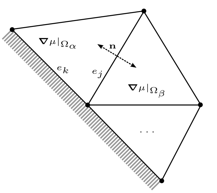
Figure 2: Triangular finite elements at a solid boundary. The value at the line segment $e_{j}$ is taken as $\nabla\mu|_{e_{j}}=0.5(\bm{\nabla}\mu|_{\Omega_{\alpha}}+\bm{\nabla}\mu|_{\Omega_{\beta}})\cdot\mathbf{n}$ and $\nabla\mu|_{e_{k}}=0$.

III Results and Discussion

III.1 Parasitic Currents

We assess the performance of the scheme by first considering a droplet with radius $R$ in a stationary flow. The average parasitic kinetic energy in the interfacial region $R\pm\xi$ of the droplet is reported in Table 1 for the mixed scheme described in Section II.3 alongside values obtained using the nodal discretization presented in our earlier work Matin et al. (2017). The mixed discretization scheme is observed to succesfully decrease the parasitic currents by two orders of magnitude compared to the nodal discretization. As outlined in Subsection II.4 this reduction is due to the piecewise constant (linear) discretization of the force terms (physical fields) that balance out the diffusion of concentration from the liquid phase to the vapor phase.

Elements	$\langle\rho\mathbf{u}\cdot\mathbf{u}\rangle_{N}$	$\langle\rho\mathbf{u}\cdot\mathbf{u}\rangle_{M}$
$1.5\cdot 10^{6}$	$0.95\cdot 10^{-6}$	$3.16\cdot 10^{-9}$
$2.9\cdot 10^{6}$	$0.14\cdot 10^{-6}$	$1.61\cdot 10^{-9}$
$4.9\cdot 10^{6}$	$0.048\cdot 10^{-6}$	$0.65\cdot 10^{-9}$

Table 1: Average parasitic kinetic energy density $\langle\rho\mathbf{u}\cdot\mathbf{u}\rangle$ in the region $R\pm\xi$ of a static droplet using the nodal $(N)$ and mixed $(M)$ scheme on different mesh resolutions. The two phases have a density contrast of $\rho_{l}/\rho_{g}=2$ and identical kinematic viscosities.

III.2 Contact Angle Measurements

We now turn to an investigation of the equilibrium shape of a three-dimensional droplet on a homogeneous surface. The droplet is initialized as a perfect hemisphere resting on a plane surface with radius $R=1$, see Fig. 3. Also illustrated is the underlying unstructured mesh. It is generated with an increasing resolution towards the bottom surface where the interface dynamics occurs, thereby enhancing the accuracy of the simulation without a significant increase in required computation time.

Figure 3: A cross section of the unstructured grid used for the droplet-simulations. The mesh contains $N=1.5\cdot 10^{6}$ grid points in total. Also shown is the initial contour $C=0.5$.

In Fig. 4(a) three equilibrium contours are shown of a droplet with a wetting potential corresponding to $\theta_{\text{eq}}=150\degree$. It is assumed that the droplet has reached equilibrium when the kinetic energy converges to a steady value asymptotically. The contact angle is then measured from the droplet height $h$ and base diameter $b$ as $\theta=\pi-\arctan(b/2(r-h))$, where $r=(4h^{2}+b^{2})/8h$. Although the interface is several lattice units thick, the measurements are performed on the contour $C=0.5$.

In Fig. 4(b) the full range of angles has been simulated by varying the wetting potential $\Omega_{c}$ for two set of density- and kinematic viscosity ratios $\{M_{\rho},\,M_{\nu}\}$ and fixed surface tension $\sigma=0.0025$. In general, we obtain good results for moderate contact angles. The largest discrepancy ($23\degree$) appears for a fully non-wet surface. For $45\lesssim\theta_{\text{eq}}\lesssim 135$ the simulated angle is within $5\degree$ of the theoretical value. It has been explicitly verified that these results are independent of the mesh resolution and interface width.

(a)

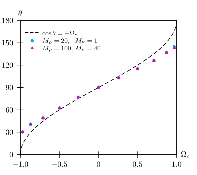
(b)

Figure 4: (a) Cross sections of the equilibrium contours ($C=0.1$, $C=0.5$ and $C=0.9$) for a droplet with $\theta_{\text{eq}}=150\degree$ and contrasts $M_{\rho}=100$ and $M_{\nu}=40$. (b) Measured equilibrium contact angle $\theta$ as a function of dimensionless wetting potential $\Omega_{c}$.

The time evolution of the kinetic energy per unit volume for $\theta_{\text{eq}}=120\degree$ is shown in Fig. 5 for different values of the mobility. Following YUE et al. (2010); Connington and Lee (2013), the effect of mobility is characterized by the dimensionless number $S=\sqrt{M\rho_{l}\nu_{l}}/R$. It is observed that the spurious currents decay at a faster rate for larger values of $S$, i.e., larger values of mobility.

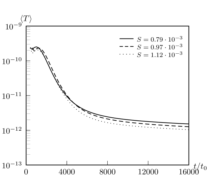
Figure 5: Time evolution of the average kinetic energy density in lattice units $\langle T\rangle=0.5\sum_{i}{(\rho_{i}\mathbf{u}_{i}\cdot\mathbf{u}_{i})}/N$ for a droplet with $M_{\rho}=100$, $M_{\nu}=40$ and fixed contact angle $\theta_{\text{eq}}=120\degree$. The mobility $M$ is varied through $S=\sqrt{M\rho_{l}\nu_{l}}/R$. Time is scaled by the viscous time $t_{0}=\rho_{l}\nu_{l}R/\sigma$.

III.3 Capillary Intrusion

We now consider the injection of a wetting liquid through a cylindrical capillary tube in order to assess whether the present FE-LBM is able to simulate correct displacement behavior and capture the capillary effect. Following the classical analysis by Washburn Washburn (1921), we neglect the viscosity of the vapor phase, gravity and intertial effects and furthermore assume that the intruding liquid is incompressible and obeys Poiseuille flow. The average flow velocity of three-dimensional Poiseuille flow is given by

$$\langle v\rangle=-\frac{(H/2)^{2}}{8\eta_{l}}\frac{dp}{dx},$$ (44)

where $H$ denotes the pipe diameter, $\eta_{l}$ the liquid dynamic viscosity and $dp/dx$ the pressure gradient that drives the liquid. The Laplace drop across a curved interface is $\Delta p=2\sigma/R$, where $\sigma$ is the surface tension between the two phases and $R$ the radius of curvature of the interface. The gradient is then $dp/dx=-2\sigma/(Rl)$, where $l$ is the length of the liquid that has penetrated the capillary. The relation between $R$ and the curvature (wetting) angle $\theta$ is $R=H/(2\cos\theta)$. By substituting these relations in Eq. (44) and using $\langle v\rangle=dy/dt$, we obtain the following equation of motion for the interface movement

$$\frac{dy}{dt}=\frac{H\sigma\cos\theta}{8\eta_{l}}.$$ (45)

The simulation setup is illustrated in Fig. 6(a). The mesh contains roughly $10^{6}$ elements and is periodic along the symmetry axis $(y)$ of the capillary. The middle portion of length $L=20H$ has no-slip wetting boundaries and the boundary conditions are periodic in all directions outside of the middle portion. Fig. 6(b) presents the results of our simulations of hydrophilic capillaries with contact angles $\theta=83\degree$, $\theta=72\degree$ and $\theta=56\degree$. The results display good agreement with theory.

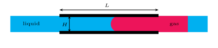
(a)

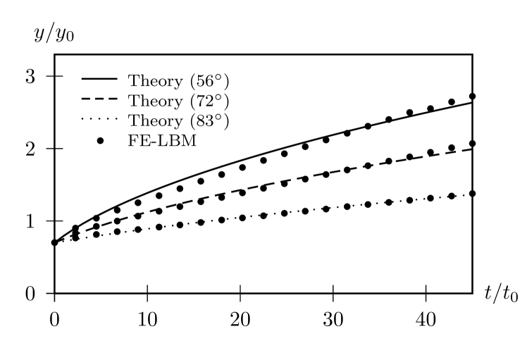
(b)

Figure 6: (a) Simulation setup for capillary intrusion. (b) The length $y/y_{0}$ of the column of the intruding liquid as a function of time $t/t_{0}$. Units are scaled by the characteristic length $y_{0}=H$ and time $t_{0}=H\eta_{l}/\sigma$.

IV Conclusion

In this study a new implementation of the FE-LBM has been developed for simulating liquid droplet behaviour on partial wetting surfaces at large density and kinematic viscosity ratios. The scheme is based on the free-energy multiphase model of Wardle and Lee Wardle and Lee (2013); Lee and Liu (2010) and augments our previous nodal-based FE-LBM formulation Matin et al. (2017) by discretizing the intermolecular forces at elements. Furthermore, the integration of the forces is now performed in the streaming step.

We have benchmarked our implementation by investigating a liquid droplet in three different settings: Immersed in a vapor phase, resting on a solid surface and moving in a capillary due to capillary pressure. The study reveals that the implementation reduces spurious currents at the interface by two orders of magnitude relative to the nodal implementation in Matin et al. (2017). Furthermore, the obtained equilibrium contact angles of the liquid droplet on a solid surface agree within $\pm 5\degree$ with the angles theoretically predicted Young’s law for partially wetting fluids ($45\lesssim\theta_{\text{eq}}\lesssim 135$).

In summary, the numerical results indicate that the present FE-LBM scheme is numerically stable and accurate and can be used to study multiphase flows where wetting effects are non-negligble, while harvesting the geometric flexibility of off-lattice schemes. Of particular interest is the effects of reservoir wettability on the relative permeabilities, which is of great importance in reservoir modelling.

V Acknowledgments

The authors acknowledge valuable discussions with Taehun Lee. This work is financed by Innovation Fund Denmark and Maersk Oil and Gas A/S through the $\text{P}^{3}$ project.

References

- Briant (2002) A. Briant, Philosophical Transactions of the Royal Society of London A: Mathematical, Physical and Engineering Sciences 360, 485 (2002).
- Briant et al. (2004) A. J. Briant, A. J. Wagner, and J. M. Yeomans, Phys. Rev. E 69, 031602 (2004).
- Briant and Yeomans (2004) A. J. Briant and J. M. Yeomans, Phys. Rev. E 69, 031603 (2004).
- Lee and Liu (2008) T. Lee and L. Liu, Phys. Rev. E 78, 017702 (2008).
- Liu and Lee (2009) L. Liu and T. Lee, International Journal of Modern Physics C 20, 1749 (2009).
- Lee and Liu (2010) T. Lee and L. Liu, Journal of Computational Physics 229, 8045 (2010).
- Connington and Lee (2013) K. Connington and T. Lee, Journal of Computational Physics 250, 601 (2013).
- Huang et al. (2007) H. Huang, D. T. Thorne, M. G. Schaap, and M. C. Sukop, Phys. Rev. E 76, 066701 (2007).
- Schmieschek and Harting (2011) S. Schmieschek and J. Harting, Communications in Computational Physics 9, 1165–1178 (2011).
- Jansen et al. (2013) H. P. Jansen, K. Sotthewes, J. van Swigchem, H. J. W. Zandvliet, and E. S. Kooij, Phys. Rev. E 88, 013008 (2013).
- Son et al. (2015) S. Son, L. Chen, D. Derome, and J. Carmeliet, Computers & Fluids 117, 42 (2015).
- Wang et al. (2013) L. Wang, H.-b. Huang, and X.-Y. Lu, Phys. Rev. E 87, 013301 (2013).
- Liu et al. (2013) H. Liu, A. J. Valocchi, Q. Kang, and C. Werth, Transport in Porous Media 99, 555 (2013).
- Ghassemi and Pak (2011) A. Ghassemi and A. Pak, Journal of Petroleum Science and Engineering 77, 135 (2011).
- Yiotis et al. (2007) A. G. Yiotis, J. Psihogios, M. E. Kainourgiakis, A. Papaioannou, and A. K. Stubos, Colloids and Surfaces A: Physicochemical and Engineering Aspects 300, 35 (2007).
- Langaas and Papatzacos (2001) K. Langaas and P. Papatzacos, Transport in Porous Media 45, 241 (2001).
- Huang and yun Lu (2009) H. Huang and X. yun Lu, Physics of Fluids 21, 092104 (2009).
- Huang et al. (2009) H. Huang, Z. Li, S. Liu, and X.-y. Lu, International Journal for Numerical Methods in Fluids 61, 341 (2009).
- Liu et al. (2015) H. Liu, Q. Kang, C. Leonardi, S. Schmieschek, A. Narváez, B. Jones, J. Williams, A. Valocchi, and J. Harting, Computational Geosciences , 1 (2015).
- Huang et al. (2015) H. Huang, C. M. Sukop, and X.-Y. Lu, Multiphase Lattice Boltzmann Methods: Theory and Application, 1st ed. (Wiley, 2015).
- Connington et al. (2015) K. W. Connington, T. Lee, and J. F. Morris, Journal of Computational Physics 283, 453 (2015).
- Rossi et al. (2005) N. Rossi, S. Ubertini, G. Bella, and S. Succi, International Journal for Numerical Methods in Fluids 49, 619 (2005).
- Patil and Lakshmisha (2009) D. V. Patil and K. Lakshmisha, Journal of Computational Physics 228, 5262 (2009).
- Misztal et al. (2015a) M. K. Misztal, A. Hernandez-Garcia, R. Matin, H. O. Sørensen, and J. Mathiesen, Journal of Computational Physics 297, 316 (2015a).
- Lee and Lin (2001) T. Lee and C.-L. Lin, Journal of Computational Physics 171, 336 (2001).
- Lee and Lin (2003) T. Lee and C.-L. Lin, Journal of Computational Physics 185, 445 (2003).
- Bardow et al. (2006) A. Bardow, I. V. Karlin, and A. A. Gusev, Europhysics Letters 75, 434 (2006).
- Misztal et al. (2015b) M. K. Misztal, A. Hernandez-Garcia, R. Matin, D. Müter, D. Jha, H. O. Sørensen, and J. Mathiesen, Frontiers in Physics 3 (2015b), 10.3389/fphy.2015.00050.
- Wardle and Lee (2013) K. E. Wardle and T. Lee, Computers and Mathematics with Applications 65, 230 (2013), special Issue on Mesoscopic Methods in Engineering and Science (ICMMES-2010, Edmonton, Canada).
- Matin et al. (2017) R. Matin, M. K. Misztal, A. Hernandez-Garcia, and J. Mathiesen, Computers & Mathematics with Applications 74, 281 (2017).
- de Gennes (1985) P. G. de Gennes, Rev. Mod. Phys. 57, 827 (1985).
- Ding and Spelt (2007) H. Ding and P. D. M. Spelt, Phys. Rev. E 75, 046708 (2007).
- Lee et al. (2006) T. Lee, C.-L. Lin, and L.-D. Chen, Journal of Computational Physics 215 (2006), 10.1016/j.jcp.2005.10.021.
- YUE et al. (2010) P. YUE, C. ZHOU, and J. J. FENG, Journal of Fluid Mechanics 645, 279–294 (2010).
- Washburn (1921) E. W. Washburn, Phys. Rev. 17, 273 (1921).