A combined analysis of PandaX, LUX, and XENON1T experiments within the framework of dark matter effective theory

Abstract

Weakly interacting massive particles are a widely well-probed dark matter candidate by the dark matter direct detection experiments. Theoretically, there are a large number of ultraviolet completed models that consist of a weakly interacting massive particle dark matter. The variety of models makes the comparison with the direct detection data complicated and often non-trivial. To overcome this, in the non-relativistic limit, the effective theory was developed in the literature which works very well to significantly reduce the complexity of dark matter-nucleon interactions and to better study the nuclear response functions. In the effective theory framework for a spin-1/2 dark matter, we combine three independent likelihood functions from the latest PandaX, LUX, and XENON1T data, and give a joint limit on each effective coupling. The astrophysical uncertainties of the dark matter distribution are also included in the likelihood. We further discuss the isospin violating cases of the interactions. Finally, for both dimension-five and dimension-six effective theories above the electroweak scale, we give updated limits of the new physics mass scales.

I Introduction

The search for particle dark matter (DM) is one of the most important topics in both particle physics and astrophysics. Yet, no clear evidence appears in direct, indirect, or collider searches of the weakly interacting massive particles (WIMPs), which are the most intriguing DM candidates as motivated by the thermal production of DM and its relic density. Instead, several stringent limits have been reported, which pushes the WIMP mass heavier or the interaction between the DM and standard model (SM) particles weaker. Among those experiments, the direct detection ones have made rapidly improved limits on probing the interaction between DM and the quark sector of SM. Such a limit from xenon-type detectors has been improved by more than one order of magnitude in recent years, from XENON100 with 34 kg target Aprile:2012nq , LUX with 250 kg Akerib:2016vxi , PandaX with 500 kg Tan:2016zwf , and finally to a ton-scale detector XENON1T Aprile:2017iyp . For a WIMP mass $m_{\chi}\sim 30\,\mathrm{GeV}$, the latest XENON1T experiment sets upper limits on the spin-independent WIMP-nucleon cross section to $\sim 10^{-46}$ cm², which is only two orders of magnitude higher than the neutrino floor.

These stringent limits constrain DM models severely. For some well-motivated DM models, the parameter space has significantly shrunk or the survival region needs to be fine-tuned, such as the blind-spot region for the neutralino DM in the supersymmetric models, (see e.g. Ref. Choudhury:2015lha ; Banerjee:2016hsk ; Han:2016qtc for the current status of the blind-spot region and Ref. Athron:2017yua ; Athron:2017qdc for the latest comprehensive global study). On the other hand, the effective theory approach begins to catch more attention, such as the spin-1 mediator models including the Anapole, magnetic dipole, and electric dipole DM. The DM dipole interaction with the SM photon can be generated by a new mediator that is kinetically mixed with the SM photon. Such a mechanism can give rise to a velocity-dependent cross section Gluscevic:2015sqa . In such a velocity-dependent framework, the published experimental limits for spin-independent and spin-dependent WIMP-nucleon cross section cannot be applied directly. Although there are many more WIMP candidate ultraviolet (UV) completed models than the given examples here, some of them may result in similar phenomena in direct detection experiments at low energies. Therefore, a model-independent limit from these experiments will be very useful to link the WIMP models with the direct detection experiments.

Regardless of the model complexity, the DM direct detection is to search for recoil events due to the WIMP scattering off nuclei inside the detector. Because of the very small momentum transfer $q\sim\mathcal{O}(\text{MeV})$ (for WIMPs) compared with mediator masses, such an interaction can be expressed using the effective field theory (EFT) whose heavier mediators can be integrated out and only a new physical scale $\Lambda$ and the information of spin and initial velocity are left. The low-energy EFT of DM has been extensively studied (e.g., see Cao:2009uw ; Goodman:2010yf ; Fan:2010gt ; Bai:2010hh ; Goodman:2010ku ; Fox:2011fx ; Fox:2011pm ; Rajaraman:2011wf ; Cheung:2012gi ; Matsumoto:2014rxa ; Hoferichter:2015ipa ; Hoferichter:2016nvd ). To study the EFT in a model independent framework, with possibly the spin and velocity dependence, a classification of 14 operators based on the spin and velocity of DM and target nuclei has been widely adopted in literature DelNobile:2013sia ; Fitzpatrick:2012ix ; Anand:2013yka ; Gresham:2014vja ; Catena:2014uqa ; Catena:2014epa ; Catena:2014hla ; Schneck:2015eqa ; Catena:2015uua ; Catena:2015vpa ; Yang:2016wrl ; Bruggisser:2016nzw ; Bishara:2016hek ; Bishara:2017nnn ; Witte:2016ydc ; Aprile:2017aas . The interaction between the DM and nuclei is generally expressed by their response functions DelNobile:2013sia ; Anand:2013yka . Any UV completed model can then be described with a combination of these 14 model-independent operators. This framework has also been adopted in studying the DM captured inside the Sun Catena:2015uha ; Liang:2016yjf ; Catena:2016ckl ; Kavanagh:2016pyr ; Catena:2016kro .

In this work, we update the current limits on the EFT operators of DM from the most recent PandaX, LUX, and XENON1T results, adopting similar methodology as that of Ref. Anand:2013yka . Comparing with previous EFT works, we have the following three main improvements. Firstly, we reconstruct three likelihoods of PandaX, LUX, and XENON1T with proper consideration of the astrophysical uncertainties. Secondly, using the reconstructed likelihood functions, we obtain combined limits on the DM mass and coupling parameters for the 14 operators as given in Ref. Anand:2013yka . For a more generic purpose, we also discuss the situation of the relativistic Lagrangian which can consist of more than one operator in the non-relativistic (NR) limit. We then discuss the isospin conserving (ISC) and isospin violating (ISV) scenarios. The ratios of maximum cancellation for ISV at the event rate level are computed. Finally, we show the updated lower bounds of new physics energy scale (or mediator mass) $\Lambda$ for dimension-five and dimension-six DM effective theories above electroweak symmetry breaking scale. The code and the likelihoods of experiments will be incorporated in the LikeDM tool Huang:2016pxg . An alternative package GAMBIT Athron:2017ard also solves the similar problems.

This paper is organized as follows. In Sec. II we briefly introduce the theory of DM direct detection in terms of effective operators. In Sec. III, we describe the experimental results of PandaX, LUX, and XENON1T, and their likelihood functions, including a detailed discussion of our treatment of the DM astrophysical parameters. In Sec. IV we present the results of our scans. We summarize our findings in Sec. V.

II DM direct detection theory

When the Earth sweeps through the local halo together with the sun, the DM from local halo may hit the underground target nuclei via the DM-nucleus scattering. The DM direct detection is designed to detect the nuclear recoil energy due to such an interaction. Unfortunately, no firm detection of such interactions has been reported in present leading xenon-target experiments, such as PandaX-II Tan:2016zwf , LUX Akerib:2016vxi , and XENON1T Aprile:2017iyp . Usually the null result is interpreted as an upper limit on the cross section of the DM-nucleon interaction, and presented separately on the spin-independent and spin-dependent components. To date, the most stringent limit on the spin-independent cross section $\sigma^{\rm{SI}}_{p}$ comes from the XENON1T experiment Aprile:2017iyp .

${\mathcal{O}}_{1}=\textbf{1}_{\chi}\textbf{1}_{N}$	${\mathcal{O}}_{9}=i{\bf{{S}}}_{\chi}\cdot\left({{\bf{S}}}_{N}\times\frac{{\bf{{q}}}}{m_{N}}\right)$
${\mathcal{O}}_{3}=i{{\bf{S}}}_{N}\cdot\left(\frac{{\bf{{q}}}}{m_{N}}\times{\bf{{v}}}^{\perp}\right)$	${\mathcal{O}}_{10}=i{{\bf{S}}}_{N}\cdot\frac{{\bf{{q}}}}{m_{N}}$
${\mathcal{O}}_{4}={{\bf{S}}}_{\chi}\cdot{{\bf{S}}}_{N}$	${\mathcal{O}}_{11}=i{\bf{{S}}}_{\chi}\cdot\frac{{\bf{{q}}}}{m_{N}}$
${\mathcal{O}}_{5}=i{\bf{{S}}}_{\chi}\cdot\left(\frac{{\bf{{q}}}}{m_{N}}\times{\bf{{v}}}^{\perp}\right)$	${\mathcal{O}}_{12}={{\bf{S}}}_{\chi}\cdot\left({{\bf{S}}}_{N}\times{\bf{{v}}}^{\perp}\right)$
${\mathcal{O}}_{6}=\left({\bf{{S}}}_{\chi}\cdot\frac{{\bf{{q}}}}{m_{N}}\right)\left({{\bf{S}}}_{N}\cdot\frac{{{\bf{q}}}}{m_{N}}\right)$	${\mathcal{O}}_{13}=i\left({{\bf{S}}}_{\chi}\cdot{\bf{{v}}}^{\perp}\right)\left({{\bf{S}}}_{N}\cdot\frac{{\bf{{q}}}}{m_{N}}\right)$
${\mathcal{O}}_{7}={{\bf{S}}}_{N}\cdot{\bf{{v}}}^{\perp}$	${\mathcal{O}}_{14}=i\left({{\bf{S}}}_{\chi}\cdot\frac{{\bf{{q}}}}{m_{N}}\right)\left({{\bf{S}}}_{N}\cdot{\bf{{v}}}^{\perp}\right)$
${\mathcal{O}}_{8}={{\bf{S}}}_{\chi}\cdot{\bf{{v}}}^{\perp}$	${\mathcal{O}}_{15}=-\left({{\bf{S}}}_{\chi}\cdot\frac{{\bf{{q}}}}{m_{N}}\right)\left[\left({{\bf{S}}}_{N}\times{\bf{{v}}}^{\perp}\right)\cdot\frac{{\bf{{q}}}}{m_{N}}\right]$

Table 1: Non-relativistic quantum mechanical operators defining the general effective theory of one-body DM-nucleon interactions. Taken from Ref. (Anand:2013yka, ).

Generally the exclusion limits by the experiment groups are based on simplified assumptions and cannot be used directly for a number of interactions. For example, a possible enhancement at small momentum transfer for the velocity dependent scattering cross section is usually not properly investigated in the standard spin-independent or spin-dependent approach by the experimental groups. To study the constraints on a variety of different operators, we adopted the particle model independent method developed in Refs. (Fitzpatrick:2012ix, ; Anand:2013yka, ). The non-relativistic quantum mechanical operators are listed in the Table 1. The operators $\mathcal{O}_{1}$ to $\mathcal{O}_{11}$ are associated with interactions of spin-0 or spin-1 mediators, while the rest are not. Because the operators in Table 1 are the mass dimension six operators, it is convenient to introduce some mass-scale parameters into the coefficients to make them dimensionless. Hence, by including the physical scale $\Lambda$ and expanding the isospin index of coefficients, one can rewrite the operator as

$$\left[\frac{c_{i}^{p}}{\Lambda^{2}}\frac{1+\tau_{3}}{2}+\frac{c_{i}^{n}}{\Lambda^{2}}\frac{1-\tau_{3}}{2}\right]\mathcal{O}_{i},$$ (1)

where $\tau_{3}$ is the 3rd Pauli matrix and $i$ runs from 1 to 15 for different operators with ${\cal O}_{2}$ omitted. Following the convention in the code DMFormFactor (Anand:2013yka, ), we set $\Lambda$ to be the Higgs vacuum expectation value $\Lambda=246\,\mathrm{GeV}$. The new coefficients $c_{i}^{p}$ and $c_{i}^{n}$ are treated as input parameters, and the relations $c_{i}^{p}=c_{i}^{n}$ and $c_{i}^{p}\neq c_{i}^{n}$ correspond to ISC and ISV scenarios, respectively.

In the limits of small recoil energy and slow DM velocity, one can expand all possible effective interactions with the following four three-vectors in the non-relativistic limit,

$${{\bf{S}}}_{\chi},\,{{\bf{S}}}_{N},\,i\frac{{\bf{{q}}}}{m_{N}},\,\,{\bf{{v}}}^{\perp},$$ (2)

where ${{\bf{S}}}_{\chi}$ and ${{\bf{S}}}_{N}$ are spins of the DM and nucleon, the vector $\bf{{q}}$ is the transfer momentum, and ${\bf{{v}}}^{\perp}$ is the velocity that is perpendicular to the momentum transfer $\bf{{q}}$. The velocity ${\bf{{v}}}^{\perp}$ is defined as ${\bf{{v}}}^{\perp}={\bf v}+{\bf q}/(2\mu_{\chi N})$ where $\mu_{\chi N}$ is the dark matter-nucleon reduced mass. In classical limits, these four three-vectors describe the states before and after a scattering. Generally speaking, if the operators are nucleon spin-dependent, the vector ${\bf{S}}_{N}$ appears in the operators whose cross sections are not coherently enhanced by a factor of target atom number square as the nucleon spin-independent case. Regarding the velocity dependent operators, they may come from the anapole or dipole interaction. For example, in Ref. Witte:2016ydc , it is shown that the anapole interaction $\bar{\chi}\gamma_{5}\chi$ depends on $\bf{q}^{2}$; the magnetic dipole interaction $\bar{\chi}\sigma^{\mu\nu}\chi$ depends on $\bf{q}^{4}$ and $(\bf{q}{\bf{v}}^{\perp})^{2}$ ($({\bf{v}}^{\perp}/\bf{q})^{2}$) for the case of mediator mass heavier (lighter) than the momentum transfer; the electric dipole interaction $\bar{\chi}\sigma^{\mu\nu}\gamma_{5}\chi$ depends on $\bf{q}^{2}$ ($\bf{q}^{-2}$) for the case of mediator mass heavier (lighter) than the momentum transfer.

Following the conventions of Ref. Catena:2015uua , we write the differential event rate of scattering between DM and the target nuclues per unit detector mass as a function of the recoil energy $Q$ as

$$\frac{{\rm d}\mathcal{R}}{{\rm d}Q} = \sum_{T}\xi_{T}\frac{\rho_{0}}{m_{\chi}m_{T}}\int_{v>v_{\rm min}(Q)}\,vf(\vec{v}+\vec{v}_{e})\frac{{\rm d}\sigma}{{\rm d}Q}\,d^{3}v,$$ (3)

where $m_{\chi}$ and $m_{T}$ are the DM and target masses. The parameter $\xi_{T}$ is defined as

$$\xi_{T}=\frac{\eta_{T}m_{T}}{\sum\limits_{T}\eta_{T}m_{T}},$$ (4)

where $\eta_{T}$ can be found in the website . The differential cross section is

$$\frac{{\rm d}\sigma}{{\rm d}Q} = \frac{m_{T}}{2\pi v^{2}}\langle|\mathcal{M}_{NR}|^{2}\rangle_{\rm spins},$$ (5)

and the averaged amplitude can be written as

$$\langle|\mathcal{M}_{NR}|^{2}\rangle_{\rm spins}=\frac{4\pi}{2J+1}\sum_{\tau,\tau^{\prime}=\{p,n\}} \bigg{[}\sum_{k=\{M,\Sigma^{\prime},\Sigma^{\prime\prime}\}}R^{\tau\tau^{\prime}}_{k}\left(v_{T}^{\perp 2},{q^{2}\over m_{N}^{2}}\right)W_{k}^{\tau\tau^{\prime}}(y)$$

$$+{q^{2}\over m_{N}^{2}}\sum_{k=\{\Phi^{\prime\prime},\Phi^{\prime\prime}M,\tilde{\Phi}^{\prime},\Delta,\Delta\Sigma^{\prime}\}}R^{\tau\tau^{\prime}}_{k}\left(v_{T}^{\perp 2},{q^{2}\over m_{N}^{2}}\right)W_{k}^{\tau\tau^{\prime}}(y)\bigg{]}\,.$$

The amplitude includes the nuclear response functions $W_{k}^{\tau\tau^{\prime}}(y)$ and the DM response functions $R^{\tau\tau^{\prime}}_{k}$, which were described in Ref. Anand:2013yka . The indices $\tau$ and $\tau^{\prime}$ run over proton $p$ and neutron $n$. We also briefly describe them in Appendix A. The symbols $M$, $\Delta$, $\Sigma^{\prime}$, $\Sigma^{\prime\prime}$, $\tilde{\Phi}^{\prime}$, and $\Phi^{\prime\prime}$ indicate the type of response function. Note that the dimension of the averaged amplitude is $\rm{mass}^{-4}$. One shall not confuse the transfer momentum $q$ in Eq. (LABEL:eq:amplitudes) with the recoil energy $Q$ in Eq. (5). These two quantities are related by $q^{2}=2m_{T}Q$.

In the astrophysics part, the DM velocity distribution function $f(\vec{v}+\vec{v}_{e})$ can be described by the Maxwell-Boltzmann distribution Lisanti:2010qx , or directly extracted from $N$-body simulation Bozorgnia:2016ogo . The Earth’s velocity in the galactic rest frame, $\vec{v}_{e}$, is added in order to translate the reference frame from the galactic rest frame to the Earth rest frame. In this work, we adopt the soft-truncated Maxwell-Boltzmann distribution Savage:2008er . The local density $\rho_{0}$ indicates the DM mass density near the Sun. We analytically integrate the velocity distribution over the solid angle and present the result in Appendix B. The minimum DM velocity can be written as a function of recoil energy, assuming that the scattering between DM and nucleus is elastic

$$v_{\rm{min}}(Q)=\sqrt{\frac{Qm_{T}}{2M_{r}^{2}}},$$ (7)

where $M_{r}$ is the reduced mass.

Finally, the efficiency of the dark matter detector $\epsilon(Q)$ needs to be included in the calculation. The total event rate is then

$$\mathcal{R}=\int^{\infty}_{0}\epsilon(Q)\frac{{\rm d}\mathcal{R}}{{\rm d}Q}dQ.$$ (8)

We will see in the following section that the event rate $\mathcal{R}$ is the best model independent quantity in our likelihood functions.

III Experimental Data and Likelihood function

III.1 PandaX-II experiment

The PandaX-II is a half-ton xenon dual-phase detector at the China Jinping underground Laboratory. The PandaX collaboration has published results based on their Run 8 (19.1 live days) and Run 9 (79.6 live days) data with exposure of 5845 kg-day and 27155 kg-day, respectively. For the Run 8, the total observed event number after all the cuts is 2 and the expected background event number is $2.4\pm 0.8$. For the Run 9, the observed event number is 1 with an expected background event number of $2.4\pm 0.7$. The $90\%$ confidence level (CL) upper limit on the $(m_{\chi},\sigma^{\rm{SI}}_{p})$ panel has been shown in Fig. 5 of Ref. Tan:2016zwf . Usually, the $90\%$ CL limit in the experimental results of the DM direct detection, is computed with the two-tail convention, which corresponds to the $95\%$ CL limit in the one-tail convention. We will adopt the one-tail convention in the analysis.

Based on the data of PandaX-II, one can simply build the likelihood function as Cheung:2012xb

$$\mathcal{L}_{\rm{PandaX}}\propto\prod_{i=\rm{run8,run9}}\max_{b_{i}^{\prime}}\frac{\exp[-(s_{i}+b_{i}^{\prime})](s_{i}+b_{i}^{\prime})^{o_{i}}}{o_{i}!}\exp\left[-\frac{(b_{i}^{\prime}-b_{i})^{2}}{2\delta b_{i}^{2}}\right],$$ (9)

where $b_{8}=b_{9}=2.4$, $\delta b_{8}=0.8$, $\delta b_{9}=0.7$, $o_{8}=2$, $o_{9}=1$. Here $s_{i}={\cal E}_{i}{\cal R}_{\text{PandaX}}$ is the theoretically predicted number of events, where ${\cal E}_{8}=5845$ kg-day, ${\cal E}_{9}=27155$ kg-day, and ${\cal R}_{\text{PandaX}}$ is computed via Eq. (8). The nuisance parameter $b_{i}^{\prime}$ is introduced for the running of pseudo-experiments. From Eq. (9), a DM model-independent likelihood function can be obtained for the PandaX experiment. Based on this pure statistical likelihood function with the $CL_{b}$ method (see Appendix  C), the $95\%$ CL upper limit on the event rate ${\cal R}_{\text{PandaX}}$ is $7.11\times 10^{-5}$ per kg-day.

Due to the complexity of the experimental performance one usually cannot exactly reproduce the $\sigma^{\rm{SI}}_{p,95\%}$ line given in Ref. Tan:2016zwf . Therefore, we introduce an additional correction factor $f(m_{\chi})$ to account for this discrepancy,

$$f(m_{\chi})\equiv\frac{s_{95}^{\rm exp}(m_{\chi})}{s_{95}^{\rm stat}}$$ (10)

where $s_{95}^{\rm exp}(m_{\chi})$ is the event number inferred from the experimental limits, the $\sigma^{\rm{SI}}_{p,95\%}$ line from Ref. Tan:2016zwf , and $s_{95}^{\rm stat}$ is the $95\%$ CL limit computed via our likelihood analysis. The default values for astrophysical parameters, quoted by Ref. Tan:2016zwf , are $v_{0}=220\,\rm{km}/s$, $\rho_{0}=0.3\,\,\mathrm{GeV}/\rm{cm}^{3}$, and $v_{esc}=544\,\rm{km}/s$. $s_{95}^{\rm stat}$ is computed by Eq. (9), which is DM model independent. Taking into account the correction factor $f(m_{\chi})$, we have

$$s_{i}(m_{\chi},\mathcal{R})=\frac{\mathcal{RE}_{i}}{f(m_{\chi})},$$ (11)

which is then used to compute the likelihood function given by Eq. (9), instead of $s_{i}={\cal RE}_{i}$ as done previously. With this correction factor included in the likelihood function, we are able to reproduce the PandaX results. Thus, in our analysis, the total likelihood of PandaX-II, $\mathcal{L}_{\rm{PandaX}}$, is a function of both $\mathcal{R}$ and $m_{\chi}$.

III.2 LUX experiment

The LUX experiment is also a dual-phase xenon (250 kg) time projection chamber. Combining two data sets WS2013 and WS2014-16, the LUX has a similar exposure ($3.35\times 10^{4}$ kg-day) to that of the PandaX, and gives comparable but slightly stronger limits (perhaps due to a different analysis method), on the DM-nucleon cross section. The LUX experiment did not report the total observed and expected events after cuts, which makes the construction of the likelihood function much more difficult. We construct a different likelihood function here than that in the PandaX case. By assuming that null signal has been detected, we build the total likelihood function of LUX as

$$\ln\mathcal{L}_{\rm{LUX}}=\sum_{i=\texttt{WS2013},\texttt{WS2014-16}}\ln\mathcal{L}_{i}(m_{\chi},\mathcal{R}),$$

$$-2\ln\mathcal{L}_{i}(m_{\chi},\mathcal{R})=\left[\frac{s_{i}(\mathcal{R})}{s_{i,{\rm{95}}}(m_{\chi})/1.64}\right]^{2},$$ (12)

where $s_{i,{\rm{95}}}(m_{\chi})$ is the number of events computed from the $95\%$ CL limit curve in Ref. Akerib:2016vxi . Here, the $95\%$ CL is equivalent to $1.64\sigma$ far from the central value in 1-dimensional Gaussian likelihood. One has to bear in mind that the theoretical prediction of the event number $s_{i}$ depends on the specific particle model of DM, because the efficiencies of WS2013 and WS2014-16 are different and it is hard to compute the likelihood in advance with a particle model-independent quantity. Hence, for the purpose of a particle model-independent study, we employ two independent $\mathcal{R}$ variables and two likelihood functions. Since the result of $\sigma^{\rm{SI}}_{p,95\%}$ of Ref. Akerib:2016vxi has been used in the likelihood Eq. (12), we do not need to consider the correction factor $f(m_{\chi})$ as in the PandaX likelihood.

III.3 XENON1T Experiment

The XENON1T Aprile:2017iyp is the first ton-scale xenon-type detector. With a fiducial mass of $\sim 1042$ kg and a running of 34.2 live days, the XENON1T data give the currently most stringent limit on the spin-independent cross section between DM and nucleon. Like PandaX and LUX, the XENON1T is also a dual-phase detector, and all the setups of the PandaX likelihood can be directly applied for XENON1T, with only the replacement of $o=1$ and $b=0.36^{+0.11}_{-0.07}$ Aprile:2017iyp . A piecewise function is used to incorporate both the positive and the negative background uncertainties. The efficiency can be found in Fig. 1 of Ref. Aprile:2017iyp . Similarly, a correction factor $f(m_{\chi})$, which is different from the one of PandaX, is needed to compensate the discrepancy between the official Xenon1T limit and our analysis.

One has to bear in mind that both XENON1T and PandaX groups used the unbinned likelihood analysis. On the contrary, our likelihood is a binned method which relies on the event number. In the binned method, all the information of each event are folded which makes our constraints weaker. Hence, our likelihood is more conservative than the actual ones by XENON1T and PandaX data.

III.4 Combined Likelihood

Before combining three experimental data sets, it is necessary to consider the shared systematical uncertainties which may be multiply counted. Since LUX, PandaX, and XENON1T are three independent experiments, the systematical uncertainties from instrumentation are expected to be independent. However, the astrophysical uncertainties of the DM distribution should be the same. They should only be considered once in the likelihood calculation.

Figure 1: Left panel: upper limits of the event rate $\mathcal{R}$ as a function of $m_{\chi}$ at $95\%$ (solid) and $99\%$ (dashed) CL, for PandaX (black), LUX (blue), and XENON1T (green). Right panel: the $95\%$ CL upper limits of $\sigma^{\rm{SI}}_{p}$ for PandaX, LUX, XENON1T, and the combination of these three experiments. Here, we adopted exactly the same astrophysical setup as used in the experimental computation, the soft-truncated Maxwell-Boltzmann distribution with $v_{0}=220\,\rm{km}/s$, $\rho_{0}=0.3\,\,\mathrm{GeV}/\rm{cm}^{3}$, and $v_{\text{esc}}=544\,\rm{km}/s$.

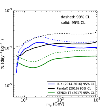
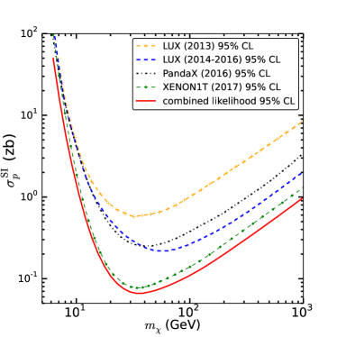
The combined likelihood can be simply written as the product of likelihoods of the three experiments, PandaX-II run8+run9 , LUX WS2013+WS2014-16, and XENON1T. In the left panel of Fig. 1, we show the upper limits of $\mathcal{R}$ at the $95\%$ (solid) and $99\%$ (dashed) CL for PandaX, LUX, and XENON1T. In all the mass region, the XENON1T limits are lower than the other two experiments. The capabilities of PandaX and LUX in constraining the DM-nucleon cross section are similar with each other, with slightly different sensitive mass regions. By comparing between the $95\%$ CL (solid) and $99\%$ CL (dashed) lines, we find that the PandaX has larger gap between the two lines than LUX, which can explain why LUX can constrain the parameter space more stringent than PandaX, although their exposure is comparable. In the right panel of Fig. 1, we give the $95\%$ CL upper limits of the spin-independent cross section based on individual likelihood and the combined one. Our combined constraint improves by a factor of $\sim 1.3$ compared with the XENON1T result.

III.5 DM astrophysical nuisance parameters

$\rho_{0}$ ($\,\mathrm{GeV}~{}\rm{cm}^{-3}$)	$0.32\pm 0.02$
$v_{0}$ (km s-1)	$240.0\pm 6.0$
$v_{\rm esc}$ (km s-1)	$541.3^{+16.6}_{-12.2}$

Table 2: The DM astrophysical nuisance parameters given in Ref. Huang:2016 which considers the rotation curve of the Milky Way within $\sim 100\,\mathrm{kpc}$.

As aforementioned, the astrophysical uncertainties have to be properly considered, particularly for the operators where the cross section is velocity dependent. The DM velocity can be simply described by a soft truncated Maxwell-Boltzmann distribution (see Eq. (27)). The parameters of the velocity distribution, the DM local velocity, the escape velocity, and the local density can be determined by the kinematics of stars or gas in the Milky Way Huang:2016 . Such methods are, however, subject to systematic uncertainties of the DM halo profile. See Ref. Read:2014qva for a compilation of the results on the local density measurements by different methods and/or data sets.

In this work we adopt the velocity parameters derived in Ref. Huang:2016 , which employed an updated precise measurement of the rotation curve using the LAMOST data to determine the DM halo properties. In Table 2, we list the parameter values and their $1\sigma$ uncertainties of the local DM density, the local DM velocity, and the escape velocity given in Ref. Huang:2016 . Unlike GAMBIT DDCalc Workgroup:2017lvb whose nuisance distribution of DM local density is log-normal, we adopt normal distribution. The uncertainties of the local velocity and escape velocity will be included in the likelihood calculation, via a profile likelihood approach.

Note that the integration of the DM velocity distribution over the solid angle is computationally heavy; we thus provide three analytical formulae valid in different velocity regions in Appendix B. The local DM density affects the normalization of the event rate. We also quote the results given in Ref. Read:2014qva , i.e., $0.20-0.56$ GeV cm^-3, which is indicated by a band in the plots of our final results.

IV Numerical results

In this section, the combined limits from the PandaX, LUX and XENON1T are presented on (i) the non-relativistic operator coefficients, (ii) the relativistic effective operator couplings, and (iii) the high energy EFT energy scale $\Lambda$. We only focus on the DM masses between $5\,\mathrm{GeV}$ and $1\,\mathrm{TeV}$. Note that our likelihood functions are particle model independent but only the spin-1/2 DM is considered in this work as illustration. For DM with different spins, the limits can be different.

We present the limits at the $95\%$ CL with the $CL_{b}$ hypothesis, namely $-2\Delta\ln\mathcal{L}=-2(\ln\mathcal{L}-\ln\mathcal{L}_{0})=2.71$. Here $\mathcal{L}_{0}$ is the likelihood without DM signal (background only hypothesis), and $\mathcal{L}$ is the corresponding likelihood for given DM model parameters. $\mathcal{L}_{0}$ is slightly smaller than the global maximal likelihood in the background-and-DM hypothesis, due to a less-than-$1\sigma$ excess for the XENON1T data. The choice of the background-only hypothesis instead of the global maximum $\mathcal{L}$ as reference makes our results more conservative.

The astrophysical parameters, including the local velocity and escape velocity, are treated as nuisance parameters following Gaussian distributions with parameters given in Table 2. As we have discussed above, a larger uncertainty band of the local density measurements  Read:2014qva is adopted to account for possible systematic uncertainties.

In many ISV studies Feng:2011vu ; Gao:2011ka ; Kumar:2011dr ; Jin:2012jn ; Okada:2013cba ; Belanger:2013tla ; Cirigliano:2013zta ; Hamaguchi:2014pja ; Zheng:2014nga ; Chen:2014tka ; Martin-Lozano:2015vva ; Yaguna:2016bga , the ISV coupling ratio for maximum cancellation between the DM-proton contribution and the DM-neutron contribution is defined at the amplitude level. Unlike such traditional definitions, we define our ISV coupling ratio for maximum cancellation at the event rate level, in which we take the experimental efficiencies and the DM velocity distribution into account. This new definition shall be more generic. As a comparison, the ISC scenario ($c_{n}=c_{p}$) is also presented.

IV.1 Non-relativistic operators

Figure 2: The combined 95% CL upper limits for non-relativistic operator coefficients of $\mathcal{O}_{1}$, $\mathcal{O}_{4}$, $\mathcal{O}_{7}$, $\mathcal{O}_{8}$, $\mathcal{O}_{10}$, and $\mathcal{O}_{11}$. The red solid lines and blue dashed lines are for the ISC and ISV scenarios, respectively. The color bands demonstrate the uncertainties of the local DM density measurements Read:2014qva .

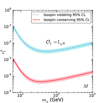
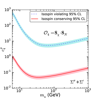
In Fig. 2, the $95\%$ upper limits for the operators that consist of only two basis three-vectors given in Eq. (2) are presented, including $\mathcal{O}_{1}$, $\mathcal{O}_{4}$, $\mathcal{O}_{7}$, $\mathcal{O}_{8}$, $\mathcal{O}_{10}$, and $\mathcal{O}_{11}$. The red solid lines are for the ISC scenario and blue dashed lines are for the ISV scenario. For convenience, we also label the response type by using the notations $M$, $\Delta$, $\Sigma^{\prime}$, $\Sigma^{\prime\prime}$, $\tilde{\Phi}^{\prime}$, and $\Phi^{\prime\prime}$, which refer to the DM current by vector charge, vector transverse magnetic, axial transverse electric, axial longitudinal, vector transverse electric, and vector longitudinal operators, respectively Anand:2013yka .

Among the operators shown on Fig. 2, only $\mathcal{O}_{1}$ and $\mathcal{O}_{4}$ are DM velocity independent operators, which correspond to the traditional spin-independent and spin-dependent interactions, respectively. The constraints on the spin-independent cross section ($\mathcal{O}_{1}$) are stronger than the spin-dependent cross section ($\mathcal{O}_{4}$), well known from previous xenon-type experiments. The limits for the nucleon spin dependent operators ($\mathcal{O}_{7}$ and $\mathcal{O}_{10}$) are always weaker than the DM spin dependent operators ($\mathcal{O}_{8}$ and $\mathcal{O}_{11}$). It can be seen from Eq. (LABEL:eq:amplitudes) and Eq. (23) that the operators $\mathcal{O}_{1}$, $\mathcal{O}_{8}$ and $\mathcal{O}_{11}$ are vector charge current interactions, and the operators $\mathcal{O}_{4}$, $\mathcal{O}_{7}$, and $\mathcal{O}_{10}$ are the axial current interactions.

Figure 3: Same as Fig. 2 but for operators $\mathcal{{O}}_{3}$, $\mathcal{{O}}_{5}$, $\mathcal{{O}}_{9}$ and $\mathcal{{O}}_{12}$.

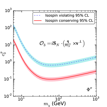
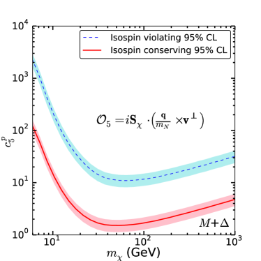
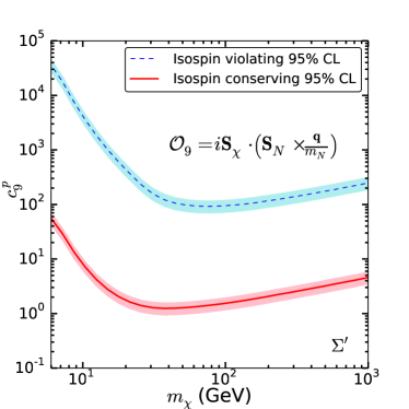
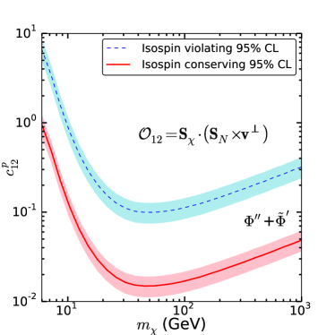
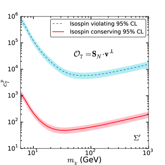
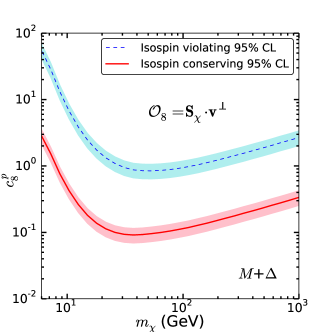
Fig. 3 shows the constraints on operators that consist of three 3-vectors, including $\mathcal{{O}}_{3}$, $\mathcal{{O}}_{5}$, $\mathcal{{O}}_{9}$ and $\mathcal{{O}}_{12}$. In contrast to Fig. 2, the limits for nucleon spin dependent operator ($\mathcal{O}_{3}$, upper left panel of Fig. 3) are stronger than the DM spin dependent one ($\mathcal{O}_{5}$, upper right panel). This is because that the contribution of the nuclear response function $\Phi^{\prime\prime}$ is larger than $M$, since $\Phi^{\prime\prime}$ possess not only the scalar contribution but also the quasicoherent one Fitzpatrick:2012ix ; Anand:2013yka . For a similar reason, the limits for $\mathcal{O}_{12}$ is two orders of magnitude stronger than that of $\mathcal{O}_{9}$, since the operator $\mathcal{O}_{12}$ also has the quasicoherent contribution from $\Phi^{\prime\prime}$.

Figure 4: Same as Fig. 2 but for operators $\mathcal{{O}}_{6}$, $\mathcal{{O}}_{13}$, $\mathcal{{O}}_{14}$ and $\mathcal{{O}}_{15}$.

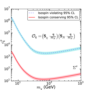
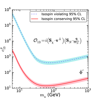
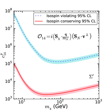
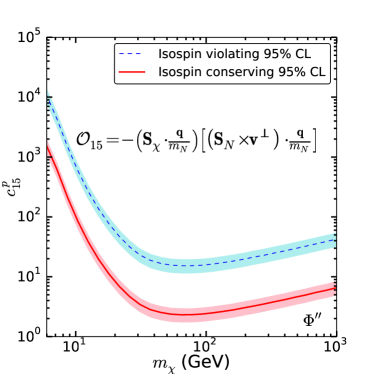
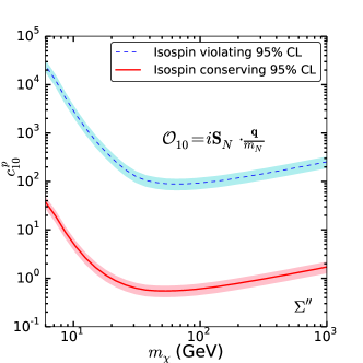
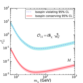
The results for the rest four operators, $\mathcal{{O}}_{6}$, $\mathcal{{O}}_{13}$, $\mathcal{{O}}_{14}$, and $\mathcal{O}_{15}$, are shown in Fig. 4. Except $\mathcal{O}_{15}$ which includes 5 basis vectors, the operators $\mathcal{{O}}_{6}$, $\mathcal{{O}}_{13}$, and $\mathcal{{O}}_{14}$ have 4 basis vectors combined. The ISC limits are similar for $\mathcal{{O}}_{6}$ and $\mathcal{{O}}_{13}$, while the ISV limits differ by about one order of magnitude for these two operators. Even though $\mathcal{{O}}_{14}$ has similar structure as $\mathcal{{O}}_{6}$ and $\mathcal{{O}}_{13}$, it behaves differently. As pointed out in Ref. (Anand:2013yka, ), the structure ${\bf{S}}_{N}\cdot{\bf{v}}^{\perp}$, where the DM couples to nucleon via the axial charge, can have a vanishing intrinsic velocity contribution so that it leads to standard spin-dependent operators. In addition, for the 5-vector combination $\mathcal{O}_{15}$, we found that the difference between ISC and ISV are the smallest among the 14 operators. This is also expected because the interference terms in $\mathcal{O}_{15}$ are from high dimensional operators.

Figure 5: The predicted ratio of the coefficient $c_{13}^{n}$ to $c_{13}^{p}$ by the minimum condition (blue dashed line) and the maximum cancellation at the $95\%$ CL (red line).

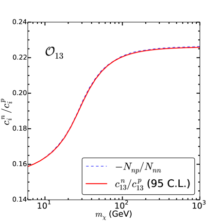
Finally, we want to discuss the ISV coupling ratio for maximum cancellation. In order to study the interference between the $\chi$-$n$ and $\chi$-$p$ amplitudes, we introduce an interference parameter $N_{np}$ and rewrite the total event number in a matrix form, as

$$N(c_{i}^{n},c_{i}^{p})=\left(\begin{array}[]{cc}c_{i}^{n}&c_{i}^{p}\end{array}\right)\left[\begin{array}[]{cc}N_{nn}&N_{np}\\ N_{np}&N_{pp}\\ \end{array}\right]\left(\begin{array}[]{ccc}c_{i}^{n}\\ c_{i}^{p}\\ \end{array}\right)\,,$$ (18)

where $N_{nn}$ is the predicted event number with $c_{i}^{n}=1$ and $c_{i}^{p}=0$, and $N_{pp}$ is the one with $c_{i}^{n}=0$ and $c_{i}^{p}=1$. The interference $N_{np}$ can be easily obtained from the numerical computation. Applying the minimum condition for the variable $c_{i}^{n}/c_{i}^{p}$, the minimum value of $N$ (maximum cancellation) is located at

$$\frac{c_{i}^{n}}{c_{i}^{p}}=-\frac{N_{np}}{N_{nn}}.$$ (19)

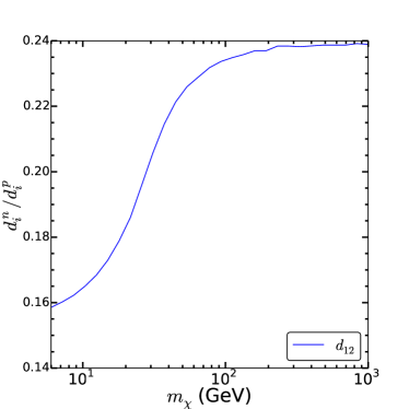
Such a coupling ratio is determined at the event level, which can slightly vary for different targets, cut efficiencies, and DM velocity distributions. In Fig. 5, we present the predicted ratio of the coefficient $c_{13}^{n}$ to $c_{13}^{p}$ by the minimum condition (blue dashed line), compared with the maximum cancellation at the $95\%$ CL (red solid line) from Fig. 4. The difference between these two is very small, suggesting that the value $-N_{np}/N_{nn}$ gives an excellent estimate of the ISV coupling ratio. One may note that the ratio becomes a constant of $0.225$ for $\mathcal{O}_{13}$ if the DM mass is much heavier than $100\,\mathrm{GeV}$.

Figure 6: The ratios the coefficients $c_{i}^{n}$ to $c_{i}^{p}$ for the other 13 operators except $\mathcal{O}_{13}$.

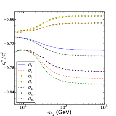
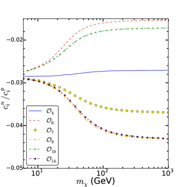
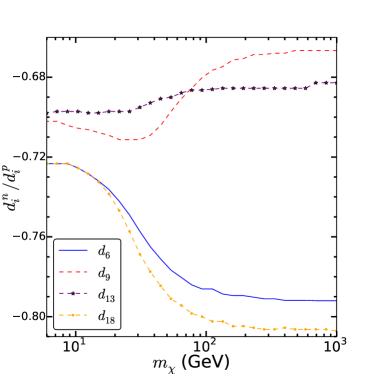
Fig. 6 shows the ratios $c_{i}^{n}/c_{i}^{p}$ for the other 13 operators except $\mathcal{O}_{13}$. We can find that such ratios for all the operators approach constant at high $m_{\chi}$ regions. The ISV coupling ratio $c_{i}^{n}/c_{i}^{p}$ is between $-0.82$ to $-0.62$ for the operators shown in the left panel of Fig. 6, and between $-0.043$ to $-0.015$ for the operators shown in the right panel. From Eq. (19), we can see that the sign of $c_{i}^{n}/c_{i}^{p}$ for the maximum cancellation is always determined by the interference term $N_{np}$. Interestingly, except for the operator $\mathcal{O}_{13}$ where the interference is negative, the interference of all the other operators is positive so that $c_{i}^{n}$ and $c_{i}^{p}$ have opposite signs for maximum ISV cancellations.

IV.2 Relativistic effective Lagrangians

Figure 7: Left panel: the 95% CL upper limits of the ISC (red solid) and ISV (blue dashed) cases for the coupling $d^{p}_{12}$. The color bands demonstrate the uncertainties of the local DM density measurements Read:2014qva . Right panel: the maximum cancellation ratio as a function of $m_{\chi}$ for $\mathcal{L}_{12}$.

Figure 8: The 95% CL upper limits of all other couplings in Eq. (20) except $d_{12}$.

In previous sections, we have mentioned that all the four-point effective Lagrangians can be expanded by the NR effective operators shown in Table 1. In fact, many relativistic Lagrangians correspond to one operator in the non-relativistic limit with a simple relationship (see Table 1 of Ref. Anand:2013yka ). For example, the ratio of $d_{3}$ (the coupling of the interaction $i\bar{\chi}\gamma_{5}\chi\bar{N}N$) to $c_{11}$ (the coefficient of the operator $i{\bf{{S}}}_{\chi}\cdot\frac{{\bf{{q}}}}{m_{N}}$) is $-m_{\chi}/m_{N}$. Again here we use the notation following Ref. Anand:2013yka . However, for some relativistic Lagrangian $\mathcal{L}_{i}$ the expansions of operators are not so trivial and may contain several operators, such as

$$d_{6}\cdot\bar{\chi}\gamma^{\mu}\chi\bar{N}i\sigma_{\mu\alpha}\frac{q^{\alpha}}{\Lambda}N \to d_{6}\cdot\left[\frac{q^{2}}{2m_{N}\Lambda}\mathcal{O}_{1}-\frac{2m_{N}}{\Lambda}\mathcal{O}_{3}+\frac{2m_{N}^{2}}{m_{\chi}\Lambda}(\frac{q^{2}}{m_{N}^{2}}\mathcal{O}_{4}-\mathcal{O}_{6})\right],$$

$$d_{7}\cdot\bar{\chi}\gamma^{\mu}\chi\bar{N}\gamma_{\mu}\gamma_{5}N \to d_{7}\cdot\left[-2\mathcal{O}_{7}+\frac{2m_{N}}{m_{\chi}}\mathcal{O}_{9}\right],$$

$$d_{9}\cdot\bar{\chi}i\sigma^{\mu\nu}\frac{q_{\nu}}{\Lambda}\chi\bar{N}\gamma_{\mu}N \to d_{9}\cdot\left[-\frac{q^{2}}{2m_{N}\Lambda}\mathcal{O}_{1}+\frac{2m_{N}}{\Lambda}\mathcal{O}_{5}-\frac{2m_{N}}{\Lambda}(\frac{q^{2}}{m_{N}^{2}}\mathcal{O}_{4}-\mathcal{O}_{6})\right],$$

$$d_{10}\cdot\bar{\chi}i\sigma^{\mu\nu}\frac{q_{\nu}}{\Lambda}\chi\bar{N}i\sigma_{\mu\alpha}\frac{q^{\alpha}}{\Lambda}N \to d_{10}\cdot\left[\frac{4q^{2}}{\Lambda^{2}}\mathcal{O}_{4}-\frac{4m_{N}^{2}}{\Lambda^{2}}\mathcal{O}_{6}\right],$$

$$d_{12}\cdot i\bar{\chi}i\sigma^{\mu\nu}\frac{q_{\nu}}{\Lambda}\chi\bar{N}i\sigma_{\mu\alpha}\frac{q^{\alpha}}{\Lambda}\gamma_{5}N \to d_{12}\cdot\left[-\frac{m_{N}}{m_{\chi}}\frac{q^{2}}{\Lambda^{2}}\mathcal{O}_{10}-4\frac{q^{2}}{\Lambda^{2}}\mathcal{O}_{12}-4\frac{m_{N}^{2}}{\Lambda^{2}}\mathcal{O}_{15}\right],$$

$$d_{13}\cdot\bar{\chi}\gamma^{\mu}\gamma_{5}\chi\bar{N}\gamma_{\mu}N \to d_{13}\cdot\left[2\mathcal{O}_{8}+2\mathcal{O}_{9}\right],$$

$$d_{18}\cdot i\bar{\chi}i\sigma^{\mu\nu}\frac{q_{\nu}}{\Lambda}\gamma_{5}\chi\bar{N}i\sigma_{\mu\alpha}\frac{q^{\alpha}}{\Lambda}N \to d_{18}\cdot\left[\frac{q^{2}}{\Lambda^{2}}\mathcal{O}_{11}+\frac{4m_{N}^{2}}{\Lambda^{2}}\mathcal{O}_{15}\right].$$ (20)

Here we omitted the energy scale $\Lambda$ in front of the interactions. It will be included in the computation as we did for the case of non-relativistic operators.

The effective Lagrangians $\mathcal{L}_{9}$ and $\mathcal{L}_{10}$ represent the magnetic dipole interaction with proton and neutron, respectively. The electric dipole moment interaction with proton is part of $\mathcal{L}_{18}$, and the Anapole interaction can be presented by $\mathcal{L}_{13}$. For more explicit expressions of the Anapole and electromagnetic moments in the effective theory, one can refer to Ref. Fitzpatrick:2012ib .

To reuse the code developed for effective operators, we can use the relationship presented in Eq. (20). Taking $\mathcal{L}_{13}$ as an example, if one sets its coupling as $d_{13}$, the coefficients of effective operators for the event rate computation are $c_{8}=2d_{13}$, $c_{9}=2d_{13}$, and the other coefficients are zero.

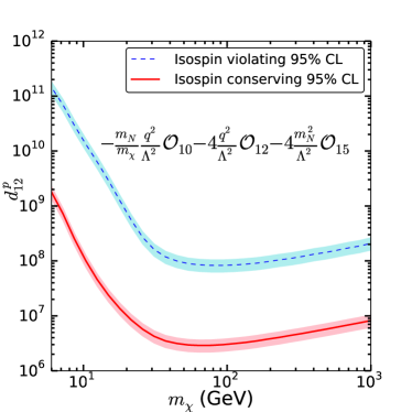
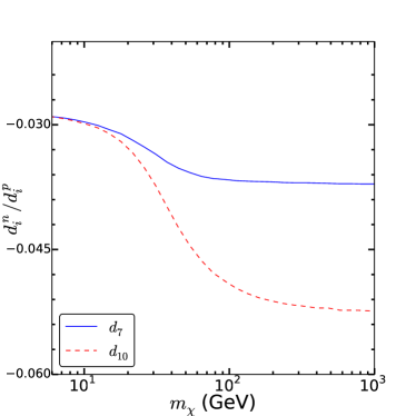
In the left panel of Fig. 7, we present the upper limits on coupling $d^{p}_{12}$ for the ISC (red solid) and ISV (blue dashed) scenarios. For the ISV scenario for all Lagrangians in Eq. (20), only the Lagrangian $\mathcal{L}_{12}$ has a positive maximum cancellation ratio. Therefore we show its results separately from the others. The maximum cancellation ratio of neutron to proton couplings for $\mathcal{L}_{12}$ as a function of $m_{\chi}$ is shown in the right panel.

Figure 9: The neutron to proton coupling ratios at the maximum cancellation for the effective Lagrangians ($i=6,7,9,10,13,18$).

The limits on the couplings for other Lagrangians are shown in Fig. 8, and the maximum cancellation ratios of neutron to proton couplings are summarized in Fig. 9.

IV.3 High energy scale theory

The new physics models beyond the standard model often appear at higher energy scale (i.e. greater than $Z$ boson mass), while the non-relativistic operators apply at the low energy scale. The match between these two scales may not be trivial. For example, the long-distance corrections due to DM scattering with a pion exchanged between two nucleons can generate a coupling $c^{i}_{p,n}$ proportional to $q^{-2}$, which would significantly change the results Fitzpatrick:2012ib ; Bishara:2016hek . In this subsection, we adopt the Mathematica package DirectDM Bishara:2016hek ; Bishara:2017nnn to calculate the relationship between the non-relativistic operators and the dimension-five and dimension-six effective DM-quark interactions. All contributions of quarks whose mass is less than $Z$ boson are included.

Figure 10: The $95\%$ CL lower limits of the energy scale $\Lambda$ for dimension-five (left) and dimension-six (right) DM-quark interactions. The color bands demonstrate the uncertainties of the local DM density measurements Read:2014qva .

Using similar conventions with that of Ref. Bishara:2016hek , we consider two dimension-five effective interactions,

$${\cal Q}_{1}^{(5)}=\frac{e}{8\pi^{2}\Lambda}(\bar{\chi}\sigma^{\mu\nu}\chi)F_{\mu\nu}\,,\qquad{\cal Q}_{2}^{(5)}=\frac{e}{8\pi^{2}\Lambda}(\bar{\chi}\sigma^{\mu\nu}i\gamma_{5}\chi)F_{\mu\nu}\,,$$ (21)

where $F_{\mu\nu}$ is the electromagnetic field strength tensor, and $\Lambda$ is the new physics energy scale. The CP even operator ${\cal Q}_{1}^{(5)}$ and the CP odd operator ${\cal Q}_{2}^{(5)}$ represent the magnetic dipole and the electric dipole interactions, respectively. Because protons and neutrons couple to the electromagnetic field differently, and there is no electric dipole interaction between DM and neutrons, the isospin is not conserved in these dimension-five interactions. The interaction ${\cal Q}_{1}^{(5)}$ can be expanded by operators with DM-proton coefficients $c^{p}_{1},c^{p}_{4},c^{p}_{5},c^{p}_{6}$ and DM-neutron coefficients $c^{n}_{4},c^{n}_{6}$, in which three coefficients $c^{p}_{5},c^{p}_{6},c^{n}_{6}$ are proportional to the inverse square of transfer momentum, $q^{-2}$. However, the interaction ${\cal Q}_{2}^{(5)}$ can only be expanded by operator $\mathcal{O}_{11}$ with the DM-proton coefficient $c^{p}_{11}$ which is also proportional to $q^{-2}$. See Appendix A of Ref. Bishara:2016hek for the exact relations.

In addition, we consider four dimension-six effective interactions between DM and quarks ($q$)

$${\cal Q}_{1,q}^{(6)} =\frac{(\bar{\chi}\gamma_{\mu}\chi)(\bar{q}\gamma^{\mu}q)}{\Lambda^{2}}, {\cal Q}_{2,q}^{(6)} =\frac{(\bar{\chi}\gamma_{\mu}\gamma_{5}\chi)(\bar{q}\gamma^{\mu}q)}{\Lambda^{2}},$$

$${\cal Q}_{3,q}^{(6)} =\frac{(\bar{\chi}\gamma_{\mu}\chi)(\bar{q}\gamma^{\mu}\gamma_{5}q)}{\Lambda^{2}}\,, {\cal Q}_{4,q}^{(6)} =\frac{(\bar{\chi}\gamma_{\mu}\gamma_{5}\chi)(\bar{q}\gamma^{\mu}\gamma_{5}q)}{\Lambda^{2}}.$$ (22)

For the sake of simplicity, we only consider the scenario where all the DM-quark couplings are unified. Therefore, isospin is conserved under such a simple assumption.

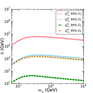
Compared with dimension-five interactions, the mappings from these four interactions to the low energy DM-nucleon coefficients do not depend on the transfer momentum. The interaction ${\cal Q}_{1,q}^{(6)}$ only relates to $c^{p,n}_{1}$. In addition to $c^{p,n}_{1}$, ${\cal Q}_{2,q}^{(6)}$ contains two more coefficients $c^{p,n}_{8}$ and $c^{p,n}_{9}$. The interaction ${\cal Q}_{3,q}^{(6)}$ has one more relevant coefficient $c^{p,n}_{7}$ added to that of ${\cal Q}_{2,q}^{(6)}$, and the interaction ${\cal Q}_{4,q}^{(6)}$ has one additional relevant coefficient $c^{p,n}_{4}$ added to that of ${\cal Q}_{3,q}^{(6)}$.

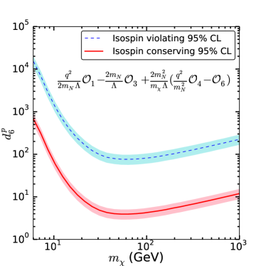
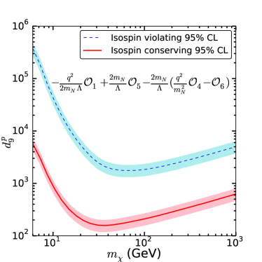
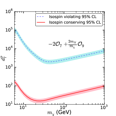
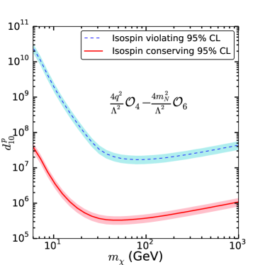
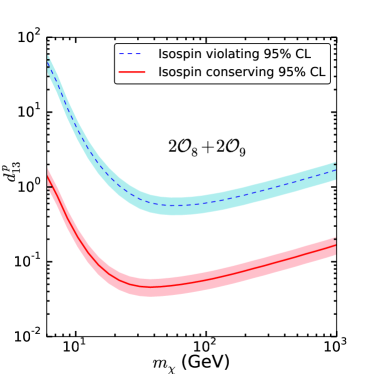
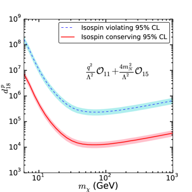
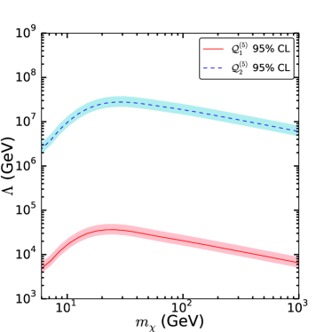
In Fig. 10, we present the $95\%$ lower limits on $\Lambda$ for dimension-five interactions (left) and dimension-six interactions (right). It is shown that the constaints on the electric dipole interaction ${\cal Q}_{2}^{(5)}$ are stronger than that of the magnetic dipole interaction ${\cal Q}_{1}^{(5)}$. The dominant operators among the six operators in ${\cal Q}_{1}^{(5)}$ NR expansion do not depend on $q^{2}$; ${\cal Q}_{2}^{(5)}$ only relates to $\mathcal{O}_{11}$ which is inversely proportional to $q^{2}$. In the right panel of Fig. 10, the interaction ${\cal Q}_{4,q}^{(6)}$ has a significant positive contribution from $\mathcal{O}_{4}$ which makes the energy scale of ${\cal Q}_{4,q}^{(6)}$ larger than that of ${\cal Q}_{3,q}^{(6)}$.

V Summary

As the first time to consider a combined analysis of three most recent and powerful experimental data sets from PandaX, LUX, and XENON1T, we have approximately reconstructed their likelihood in terms of event rates and reported a new combined limit based on a spin-1/2 DM. To consider the possible impact of astrophysical uncertainties from the DM local velocity, escape velocity, and local density, we introduce these parameters as nuisance parameters in our likelihood.

In the low energy effective operator framework, we apply our combined likelihood for each effective operator and derive their $95\%$ CL upper limits on the plane ($m_{\chi}$, $c_{i}^{p}$) for the ISC and ISV (with maximum cancellations) scenarios. As expected, our combined limits of the effective operators are more stringent than previous studies Fitzpatrick:2012ib ; Catena:2015uua . In addition to the low energy effective operator framework, we also study the high energy effective Lagrangians which can usually be expressed as the combination of several operators. The $95\%$ CL limits (upper or lower) on the ($m_{\chi}$, $d_{i}^{p}$) and ($m_{\chi}$, $\Lambda$) planes are presented with several representative high energy effective Lagrangians.

The inclusion of the uncertainties of the DM velocity distribution and the escape velocity of the solar location leads to $\lesssim 5\%$ uncertainties for the velocity independent operators and $\lesssim 7.5\%$ for the velocity dependent operators. The maximum uncertainties appear around $m_{\chi}\lesssim 10\,\mathrm{GeV}$ whose recoil energies fall into the small efficiency region. However, such astrophysical parameters depend on the data sets and modeling of the luminous matter distribution, as well as the prior assumption of the DM density profile, which may be subject to additional systematic uncertainties. Therefore we quote a relatively large band of the local DM density measured by different analyses Read:2014qva to show a potential uncertainty range of our results.

For the xenon target detectors, we report new ISV coupling ratios $c_{i}^{n}/c_{i}^{p}$ for the maximum cancellation between the contributions of DM-proton and DM-neutron couplings. Firstly, we find that the ratio is not a constant with respect to the DM mass. However, as long as the DM mass is heavy, the ratio asymptotically approaches a constant. Secondly, only the operator $\mathcal{O}_{13}$ has a positive ratio, and the rest operators have negative ratios for the maximum cancellation. Finally, the well-known number of $c_{i}^{n}/c_{i}^{p}=-0.7$ only agrees with the operators $\mathcal{O}_{i=1,3,5,8,11,12,15}$. For the high energy effective Lagrangian cases, only the transfer momentum dependent operators can have a large ratio change with respect to the DM mass. The ratios are between their compositions of lower energy operators. In this paper, we only studied one-nucleon contributions. If the two-nucleon correlations would be included, the result of ISV case can be changed Cirigliano:2013zta ; Korber:2017ery .

Lastly, we would like to suggest the future experiments to publish their limits of event rates $\mathcal{R}$ togehter with the spin-independent and spin-dependent cross sections. There are two advantages to present the limits on the plane ($m_{\chi}$, $\mathcal{R}$). Firstly, this can help theorists to go beyond the neutralino-like benchmark scenario which is only relevant to operators $\mathcal{O}_{1}$ and $\mathcal{O}_{4}$. As performed by the SuperCDMS collaboration Schneck:2015eqa and XENON collaboration Aprile:2017aas , the EFT operators can provide a more general framework to explore the DM-nuclear interaction. With the likelihood information of $\mathcal{R}$, one can simply obtain the experimental limits for their interested operators. Secondly, it also helps to unfold the astrophysical uncertainties. The systematic uncertainties for the next generation DM direct detection detectors will be more important because the statistical precision can be much improved for the future ton-scale detectors and more kinematic information can be obtained for example in the DM directional detection experiments.

Appendix A DM response function

Following the definition of Ref. Anand:2013yka , we use the notations $M$, $\Delta$, $\Sigma^{\prime}$, $\Sigma^{\prime\prime}$, $\tilde{\Phi}^{\prime}$, and $\Phi^{\prime\prime}$ to represent the DM currents by the vector charge, vector transverse magnetic, axial transverse electric, axial longitudinal, vector transverse electric, and vector longitudinal operators, respectively. In the DM response functions, one needs also to consider two interference terms, $\Phi^{\prime\prime}M$ and $\Delta\Sigma^{\prime}$. There are eight possible DM response functions:

$$R_{M}^{\tau\tau^{\prime}}\left(v_{T}^{\perp 2},{q^{2}\over m_{N}^{2}}\right) = c_{1}^{\tau}c_{1}^{\tau^{\prime}}+{j_{\chi}(j_{\chi}+1)\over 3}\left[{q^{2}\over m_{N}^{2}}v_{T}^{\perp 2}c_{5}^{\tau}c_{5}^{\tau^{\prime}}+v_{T}^{\perp 2}c_{8}^{\tau}c_{8}^{\tau^{\prime}}+{q^{2}\over m_{N}^{2}}c_{11}^{\tau}c_{11}^{\tau^{\prime}}\right]$$

$$R_{\Phi^{\prime\prime}}^{\tau\tau^{\prime}}\left(v_{T}^{\perp 2},{q^{2}\over m_{N}^{2}}\right) = {q^{2}\over 4m_{N}^{2}}c_{3}^{\tau}c_{3}^{\tau^{\prime}}+{j_{\chi}(j_{\chi}+1)\over 12}\left(c_{12}^{\tau}-{q^{2}\over m_{N}^{2}}c_{15}^{\tau}\right)\left(c_{12}^{\tau^{\prime}}-{q^{2}\over m_{N}^{2}}c_{15}^{\tau^{\prime}}\right)$$

$$R_{\Phi^{\prime\prime}M}^{\tau\tau^{\prime}}\left(v_{T}^{\perp 2},{q^{2}\over m_{N}^{2}}\right) = c_{3}^{\tau}c_{1}^{\tau^{\prime}}+{j_{\chi}(j_{\chi}+1)\over 3}\left(c_{12}^{\tau}-{q^{2}\over m_{N}^{2}}c_{15}^{\tau}\right)c_{11}^{\tau^{\prime}}$$

$$R_{\tilde{\Phi}^{\prime}}^{\tau\tau^{\prime}}\left(v_{T}^{\perp 2},{q^{2}\over m_{N}^{2}}\right) = {j_{\chi}(j_{\chi}+1)\over 12}\left[c_{12}^{\tau}c_{12}^{\tau^{\prime}}+{q^{2}\over m_{N}^{2}}c_{13}^{\tau}c_{13}^{\tau^{\prime}}\right]$$

$$R_{\Sigma^{\prime\prime}}^{\tau\tau^{\prime}}\left(v_{T}^{\perp 2},{q^{2}\over m_{N}^{2}}\right) = {q^{2}\over 4m_{N}^{2}}c_{10}^{\tau}c_{10}^{\tau^{\prime}}+{j_{\chi}(j_{\chi}+1)\over 12}\left[c_{4}^{\tau}c_{4}^{\tau^{\prime}}+\right.$$

$$\left.{q^{2}\over m_{N}^{2}}(c_{4}^{\tau}c_{6}^{\tau^{\prime}}+c_{6}^{\tau}c_{4}^{\tau^{\prime}})+{q^{4}\over m_{N}^{4}}c_{6}^{\tau}c_{6}^{\tau^{\prime}}+v_{T}^{\perp 2}c_{12}^{\tau}c_{12}^{\tau^{\prime}}+{q^{2}\over m_{N}^{2}}v_{T}^{\perp 2}c_{13}^{\tau}c_{13}^{\tau^{\prime}}\right]$$

$$R_{\Sigma^{\prime}}^{\tau\tau^{\prime}}\left(v_{T}^{\perp 2},{q^{2}\over m_{N}^{2}}\right) = {1\over 8}\left[{q^{2}\over m_{N}^{2}}v_{T}^{\perp 2}c_{3}^{\tau}c_{3}^{\tau^{\prime}}+v_{T}^{\perp 2}c_{7}^{\tau}c_{7}^{\tau^{\prime}}\right]+{j_{\chi}(j_{\chi}+1)\over 12}\left[c_{4}^{\tau}c_{4}^{\tau^{\prime}}+\right.$$

$$\left.{q^{2}\over m_{N}^{2}}c_{9}^{\tau}c_{9}^{\tau^{\prime}}+{v_{T}^{\perp 2}\over 2}\left(c_{12}^{\tau}-{q^{2}\over m_{N}^{2}}c_{15}^{\tau}\right)\left(c_{12}^{\tau^{\prime}}-{q^{2}\over m_{N}^{2}}c_{15}^{\tau\prime}\right)+{q^{2}\over 2m_{N}^{2}}v_{T}^{\perp 2}c_{14}^{\tau}c_{14}^{\tau^{\prime}}\right]$$

$$R_{\Delta}^{\tau\tau^{\prime}}\left(v_{T}^{\perp 2},{q^{2}\over m_{N}^{2}}\right) = {j_{\chi}(j_{\chi}+1)\over 3}\left[{q^{2}\over m_{N}^{2}}c_{5}^{\tau}c_{5}^{\tau^{\prime}}+c_{8}^{\tau}c_{8}^{\tau^{\prime}}\right]$$

$$R_{\Delta\Sigma^{\prime}}^{\tau\tau^{\prime}}\left(v_{T}^{\perp 2},{q^{2}\over m_{N}^{2}}\right) = {j_{\chi}(j_{\chi}+1)\over 3}\left[c_{5}^{\tau}c_{4}^{\tau^{\prime}}-c_{8}^{\tau}c_{9}^{\tau^{\prime}}\right].$$ (23)

Appendix B Integration of the DM velocity distribution over solid angle

From the differential event rate Eq. (3), one can compute the solid angle integration part first, namely

$$\int_{v>v_{\rm min}(Q)}v^{3}dv\int_{0}^{2\pi}d\varphi\int_{0}^{\pi}\frac{{\rm d}\sigma}{{\rm d}Q}f(\vec{v}+\vec{v}_{e})\sin\theta d\theta,$$ (24)

where $\varphi$ and $\theta$ are the azimuthal angle and polar angle in the Earth frame. Because $\frac{{\rm d}\sigma}{{\rm d}Q}$ does not depend on $\theta$ and $\varphi$, we can rewrite Eq. (24) as

$$\int_{v>v_{\rm min}(Q)}v^{3}\frac{{\rm d}\sigma}{{\rm d}Q}\times I(\vec{v}+\vec{v}_{e})dv,$$ (25)

where

$$I(\vec{v}+\vec{v}_{e})\equiv\int_{0}^{2\pi}d\varphi\int_{0}^{\pi}f(\vec{v}+\vec{v}_{e})\sin\theta d\theta.$$ (26)

We adopt the soft truncated Maxwell-Boltzmann distribution of $f$:

$$f(\vec{v}+\vec{v}_{e})=\frac{(e^{-{(\vec{v}+\vec{v}_{e})^{2}}/{v_{0}^{2}}}-e^{-{v_{\text{esc}}^{2}}/{v_{0}^{2}}})\Theta(v_{\text{esc}}^{2}-(\vec{v}+\vec{v}_{e})^{2})}{\pi^{3/2}v_{0}^{3}\times\rm{Norm}},$$ (27)

where $\Theta(x)$ is the step function, and “Norm” is the normalization factor

$${\rm erf}\left(\frac{v_{\text{esc}}}{v_{0}}\right)-\left[\frac{4}{3\sqrt{\pi}}\left(\frac{v_{\text{esc}}}{v_{0}}\right)^{3}+\frac{2v_{\text{esc}}}{\sqrt{\pi}v_{0}}\right]\exp\left(-\frac{v_{\text{esc}}^{2}}{v_{0}^{2}}\right).$$

In the above formulae, $v_{0}$, $v_{e}$ and $v_{\text{esc}}$ are all in the Galactic center (GC) frame.

The relationship between the DM velocity $\vec{v}+\vec{v}_{e}$ in the GC frame and the velocity magnitude $v$ in the Earth frame is

$$\vec{v}+\vec{v}_{e}=(v\sin\theta\cos\varphi,v\sin\theta\sin\varphi,v\cos\theta+v_{e}).$$

Note that we set $\vec{v_{z}}$ to be parallel to $\vec{v_{e}}$. Hence, the integration of angle $\varphi$ in Eq. (26) can be done prior to $\theta$, which gives a prefactor $2\pi$. Finally, we can integrate $I(\vec{v}+\vec{v}_{e})$ over the angle $\theta$ in terms of variables $a=v_{\text{esc}}/v_{0}$, $b=v_{e}/v_{0}$, and $x=v/v_{0}$. We find that $I(\vec{v}+\vec{v}_{e})$ has 3 types of solutions, depending on the relationships between $a$, $b$ and $x$.

1. Region $x+b<a$ or $v+v_{e}<v_{esc}$:

   $$I=\frac{e^{-(x+b)^{2}}\left[3e^{a^{2}}\left(e^{4xb}-1\right)-12xbe^{(x+b)^{2}}\right]}{xbv_{0}^{3}\left[3\sqrt{\pi}e^{a^{2}}{\rm erf}\left(a\right)-6a-4a^{3}\right]}.$$

2. Region ($x+b>a$, $|x-b|<a$) or ($v+v_{e}>v_{esc}$, $|v-v_{e}|<v_{esc}$):

   $$I=\frac{3\left[e^{a^{2}-(x-b)^{2}}+(x-b)^{2}-a^{2}-1\right]}{xbv_{0}^{3}\left[3\sqrt{\pi}e^{a^{2}}{\rm erf}\left(a\right)-6a-4a^{3}\right]}.$$

3. Region $|x-b|>a$ or $|v-v_{e}|>v_{esc}$:

   $$I=0.$$

Appendix C Confidence limits

To determine the exclusion limits, a confidence level ($CL$) is usually used, defined as

$$1-CL=\int_{\chi^{2}_{c}}^{\infty}\mathcal{L}(\chi^{2})d\chi^{2},$$ (28)

where the desired $CL$ value is the integral likelihood for the range $0<\chi^{2}<\chi^{2}_{c}$. If the likelihood $\mathcal{L}$ is Gaussian distribution ($\propto\exp(-\chi^{2}/2)$), then we can simply obtain $\chi^{2}_{c}=2.71$ at $CL=0.95$ (one sided confidence limit). Using such a definition, conventionally we can describe the consistency of the data with the background-only hypothesis $CL_{b}$ and the signal-plus-background hypothesis $CL_{s+b}$.

However, in many real cases one can introduce nuisance parameters and model parameters to the likelihood function as systematic uncertainties which makes it difficult to find $CL_{b}$ and $CL_{s+b}$ by integrating the multi-dimensional parameter space in Eq. (28). Therefore, it is convenient to introduce a test-statistic $\chi^{2}(s,b)=-2\ln\mathcal{L}(s,b)$ to numerically pin down the confidence level for two hypotheses of background-only and signal-plus-background.

In the $m_{\chi}-\mathcal{R}$ plane, we divide $m_{\chi}$ into various bins. For each $m_{\chi}$ bin, the $\chi^{2}$ varies as a function of $\mathcal{R}$. Then, we solve the following equation

$$\Delta\chi^{2}=\chi^{2}(m_{\chi},\mathcal{R})-\chi^{2}(m_{\chi},\mathcal{R}=0)=2.71,$$ (29)

to get a value of $\mathcal{R}_{95}$ corresponding to the 95% upper limits based on the $CL_{b}$ method. Repeating the process for different $m_{\chi}$ bins, we can get a curve on the $m_{\chi}-\mathcal{R}_{95}$ plane corresponding to the 95% exclusion limit.

Regarding to $CL_{s+b}$ method, the same procedure as described above can be performed, but solving a different equation

$$\Delta\chi^{2}=\chi^{2}(m_{\chi},\mathcal{R})-\chi^{2}_{\rm min}(m_{\chi},\mathcal{R})=2.71$$ (30)

to get the $\mathcal{R}_{95}$ limits.

Since we are using the null hypothesis (background only), we adopt the $CL_{b}$ method to evaluate the limits. It is worthy mentioning that our limits will be hence slightly weaker than the $CL_{s+b}$ method.

Appendix D Limit including PandaX run10 data

Figure 11: Left panel: the $95\%$ CL upper limits of $\sigma^{\rm{SI}}_{p}$ for new combined likelihood (red solid line) and old combined likelihood (blue dashed line). Right panel: the $95\%$ CL upper limits of $c_{i}^{p}$ for $\mathcal{O}_{1}$ and $\mathcal{O}_{4}$ (ISC). In both panels, the solid lines are for the old combined likelihood but dash lines are the new one.

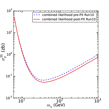
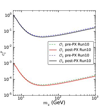
In this appendix, we will show the update limit including the latest PandaX run9^′+run10 data Cui:2017nnn . For the new Run9^′, the total observed event number after all the cuts is 1 and the expected background event number is $3.2\pm 0.9$. For the Run10, there is none observed event number but the expected background event number is $1.8\pm 0.5$. With the updated exposure ${\cal E}_{9}=26180.44$ kg-day and ${\cal E}_{10}=27871.65$ kg-day, we replace the old PandaX likelihood (run8+run9) to new one (run9^′+run10) in the Fig. 11. One can see that the improvement is around $20\%$ in the spin independent cross section but it is not significant in the ($m_{\chi}$, $c_{i}^{p}$) plane.

References

- [1] E. Aprile et al. [XENON100 Collaboration], Phys. Rev. Lett. 109 (2012) 181301 doi:10.1103/PhysRevLett.109.181301 [arXiv:1207.5988 [astro-ph.CO]].
- [2] D. S. Akerib et al. [LUX Collaboration], Phys. Rev. Lett. 118, no. 2, 021303 (2017) doi:10.1103/PhysRevLett.118.021303 [arXiv:1608.07648 [astro-ph.CO]].
- [3] A. Tan et al. [PandaX-II Collaboration], Phys. Rev. Lett. 117 (2016) no.12, 121303 doi:10.1103/PhysRevLett.117.121303 [arXiv:1607.07400 [hep-ex]].
- [4] E. Aprile et al., arXiv:1705.06655 [astro-ph.CO].
- [5] A. Choudhury, K. Kowalska, L. Roszkowski, E. M. Sessolo and A. J. Williams, JHEP 1604, 182 (2016) doi:10.1007/JHEP04(2016)182 [arXiv:1509.05771 [hep-ph]].
- [6] S. Banerjee, S. Matsumoto, K. Mukaida and Y. L. S. Tsai, JHEP 1611, 070 (2016) doi:10.1007/JHEP11(2016)070 [arXiv:1603.07387 [hep-ph]].
- [7] T. Han, F. Kling, S. Su and Y. Wu, JHEP 1702, 057 (2017) doi:10.1007/JHEP02(2017)057 [arXiv:1612.02387 [hep-ph]].
- [8] P. Athron et al. [GAMBIT Collaboration], arXiv:1705.07935 [hep-ph].
- [9] P. Athron et al. [GAMBIT Collaboration], arXiv:1705.07917 [hep-ph].
- [10] V. Gluscevic, M. I. Gresham, S. D. McDermott, A. H. G. Peter and K. M. Zurek, JCAP 1512 (2015) no.12, 057 doi:10.1088/1475-7516/2015/12/057 [arXiv:1506.04454 [hep-ph]].
- [11] Q. H. Cao, C. R. Chen, C. S. Li and H. Zhang, JHEP 1108 (2011) 018 doi:10.1007/JHEP08(2011)018 [arXiv:0912.4511 [hep-ph]].
- [12] J. Goodman, M. Ibe, A. Rajaraman, W. Shepherd, T. M. P. Tait and H. B. Yu, Phys. Lett. B 695 (2011) 185 doi:10.1016/j.physletb.2010.11.009 [arXiv:1005.1286 [hep-ph]].
- [13] J. Fan, M. Reece and L. T. Wang, JCAP 1011, 042 (2010) doi:10.1088/1475-7516/2010/11/042 [arXiv:1008.1591 [hep-ph]].
- [14] Y. Bai, P. J. Fox and R. Harnik, JHEP 1012 (2010) 048 doi:10.1007/JHEP12(2010)048 [arXiv:1005.3797 [hep-ph]].
- [15] J. Goodman, M. Ibe, A. Rajaraman, W. Shepherd, T. M. P. Tait and H. B. Yu, Phys. Rev. D 82 (2010) 116010 doi:10.1103/PhysRevD.82.116010 [arXiv:1008.1783 [hep-ph]].
- [16] P. J. Fox, R. Harnik, J. Kopp and Y. Tsai, Phys. Rev. D 84 (2011) 014028 doi:10.1103/PhysRevD.84.014028 [arXiv:1103.0240 [hep-ph]].
- [17] P. J. Fox, R. Harnik, J. Kopp and Y. Tsai, Phys. Rev. D 85 (2012) 056011 doi:10.1103/PhysRevD.85.056011 [arXiv:1109.4398 [hep-ph]].
- [18] A. Rajaraman, W. Shepherd, T. M. P. Tait and A. M. Wijangco, Phys. Rev. D 84 (2011) 095013 doi:10.1103/PhysRevD.84.095013 [arXiv:1108.1196 [hep-ph]].
- [19] K. Cheung, P. Y. Tseng, Y. L. S. Tsai and T. C. Yuan, JCAP 1205 (2012) 001 doi:10.1088/1475-7516/2012/05/001 [arXiv:1201.3402 [hep-ph]].
- [20] S. Matsumoto, S. Mukhopadhyay and Y. L. S. Tsai, JHEP 1410 (2014) 155 doi:10.1007/JHEP10(2014)155 [arXiv:1407.1859 [hep-ph]].
- [21] M. Hoferichter, P. Klos and A. Schwenk, Phys. Lett. B 746 (2015) 410 doi:10.1016/j.physletb.2015.05.041 [arXiv:1503.04811 [hep-ph]].
- [22] M. Hoferichter, P. Klos, J. Menéndez and A. Schwenk, Phys. Rev. D 94 (2016) no.6, 063505 doi:10.1103/PhysRevD.94.063505 [arXiv:1605.08043 [hep-ph]].
- [23] M. Cirelli, E. Del Nobile and P. Panci, JCAP 1310 (2013) 019 doi:10.1088/1475-7516/2013/10/019 [arXiv:1307.5955 [hep-ph]].
- [24] A. L. Fitzpatrick, W. Haxton, E. Katz, N. Lubbers and Y. Xu, JCAP 1302 (2013) 004 doi:10.1088/1475-7516/2013/02/004 [arXiv:1203.3542 [hep-ph]].
- [25] N. Anand, A. L. Fitzpatrick and W. C. Haxton, Phys. Rev. C 89, no. 6, 065501 (2014) doi:10.1103/PhysRevC.89.065501 [arXiv:1308.6288 [hep-ph]].
- [26] M. I. Gresham and K. M. Zurek, Phys. Rev. D 89 (2014) no.12, 123521 doi:10.1103/PhysRevD.89.123521 [arXiv:1401.3739 [hep-ph]].
- [27] R. Catena and P. Gondolo, JCAP 1409, no. 09, 045 (2014) doi:10.1088/1475-7516/2014/09/045 [arXiv:1405.2637 [hep-ph]].
- [28] R. Catena, JCAP 1407 (2014) 055 doi:10.1088/1475-7516/2014/07/055 [arXiv:1406.0524 [hep-ph]].
- [29] R. Catena, JCAP 1409 (2014) no.09, 049 doi:10.1088/1475-7516/2014/09/049 [arXiv:1407.0127 [hep-ph]].
- [30] K. Schneck et al. [SuperCDMS Collaboration], Phys. Rev. D 91 (2015) no.9, 092004 doi:10.1103/PhysRevD.91.092004 [arXiv:1503.03379 [astro-ph.CO]].
- [31] E. Aprile et al. [XENON Collaboration], Phys. Rev. D 96 (2017) no.4, 042004 doi:10.1103/PhysRevD.96.042004 [arXiv:1705.02614 [astro-ph.CO]].
- [32] R. Catena and P. Gondolo, JCAP 1508, no. 08, 022 (2015) doi:10.1088/1475-7516/2015/08/022 [arXiv:1504.06554 [hep-ph]].
- [33] R. Catena, JCAP 1507 (2015) no.07, 026 doi:10.1088/1475-7516/2015/07/026 [arXiv:1505.06441 [hep-ph]].
- [34] K. C. Yang, Phys. Rev. D 94 (2016) no.3, 035028 doi:10.1103/PhysRevD.94.035028 [arXiv:1604.04979 [hep-ph]].
- [35] S. Bruggisser, F. Riva and A. Urbano, JHEP 1611 (2016) 069 doi:10.1007/JHEP11(2016)069 [arXiv:1607.02475 [hep-ph]].
- [36] F. Bishara, J. Brod, B. Grinstein and J. Zupan, JCAP 1702 (2017) no.02, 009 doi:10.1088/1475-7516/2017/02/009 [arXiv:1611.00368 [hep-ph]].
- [37] F. Bishara, J. Brod, B. Grinstein and J. Zupan, arXiv:1708.02678 [hep-ph].
- [38] S. J. Witte, V. Gluscevic and S. D. McDermott, JCAP 1702 (2017) no.02, 044 doi:10.1088/1475-7516/2017/02/044 [arXiv:1612.07808 [hep-ph]].
- [39] B. A. Dobrescu and I. Mocioiu, JHEP 0611 (2006) 005 doi:10.1088/1126-6708/2006/11/005 [hep-ph/0605342].
- [40] R. Catena and B. Schwabe, JCAP 1504 (2015) no.04, 042 doi:10.1088/1475-7516/2015/04/042 [arXiv:1501.03729 [hep-ph]].
- [41] Z. L. Liang, Y. L. Wu, Z. Q. Yang and Y. F. Zhou, JCAP 1609 (2016) no.09, 018 doi:10.1088/1475-7516/2016/09/018 [arXiv:1606.02157 [hep-ph]].
- [42] R. Catena and A. Widmark, JCAP 1612 (2016) no.12, 016 doi:10.1088/1475-7516/2016/12/016 [arXiv:1609.04825 [astro-ph.CO]].
- [43] B. J. Kavanagh, R. Catena and C. Kouvaris, JCAP 1701 (2017) no.01, 012 doi:10.1088/1475-7516/2017/01/012 [arXiv:1611.05453 [hep-ph]].
- [44] R. Catena, JCAP 1701 (2017) no.01, 059 doi:10.1088/1475-7516/2017/01/059 [arXiv:1609.08967 [astro-ph.CO]].
- [45] X. Huang, Y. L. S. Tsai and Q. Yuan, Comput. Phys. Commun. 213, 252 (2017) doi:10.1016/j.cpc.2016.12.015 [arXiv:1603.07119 [hep-ph]].
- [46] P. Athron et al. [GAMBIT Collaboration], arXiv:1705.07908 [hep-ph].
- [47] M. Lisanti, L. E. Strigari, J. G. Wacker and R. H. Wechsler, Phys. Rev. D 83, 023519 (2011) doi:10.1103/PhysRevD.83.023519 [arXiv:1010.4300 [astro-ph.CO]].
- [48] N. Bozorgnia et al., JCAP 1605, no. 05, 024 (2016) doi:10.1088/1475-7516/2016/05/024 [arXiv:1601.04707 [astro-ph.CO]].
- [49] C. Savage, G. Gelmini, P. Gondolo and K. Freese, JCAP 0904, 010 (2009) doi:10.1088/1475-7516/2009/04/010 [arXiv:0808.3607 [astro-ph]].
- [50] K. Cheung, Y. L. S. Tsai, P. Y. Tseng, T. C. Yuan and A. Zee, JCAP 1210 (2012) 042 doi:10.1088/1475-7516/2012/10/042 [arXiv:1207.4930 [hep-ph]].
- [51] X. Cui et al. [PandaX-II Collaboration], arXiv:1708.06917 [astro-ph.CO].
- [52] Y. Huang, X. Liu, H. Yuan, M. Xiang, H. Zhang, B. Chen, J. Ren, C. Wang, Y. Zhang, Y. Hou, Y. Wang, and Z. Cao. Mon. Not.Roy. Astron. Soc., 463, 2623 [arXiv:1604.01216]
- [53] J. I. Read, J. Phys. G 41 (2014) 063101 doi:10.1088/0954-3899/41/6/063101 [arXiv:1404.1938 [astro-ph.GA]].
- [54] T. Bringmann et al. [GAMBIT Dark Matter Workgroup], arXiv:1705.07920 [hep-ph].
- [55] J. L. Feng, J. Kumar, D. Marfatia and D. Sanford, Phys. Lett. B 703, 124 (2011) doi:10.1016/j.physletb.2011.07.083 [arXiv:1102.4331 [hep-ph]].
- [56] X. Gao, Z. Kang and T. Li, JCAP 1301, 021 (2013) doi:10.1088/1475-7516/2013/01/021 [arXiv:1107.3529 [hep-ph]].
- [57] J. Kumar, D. Sanford and L. E. Strigari, Phys. Rev. D 85, 081301 (2012) doi:10.1103/PhysRevD.85.081301 [arXiv:1112.4849 [astro-ph.CO]].
- [58] H. B. Jin, S. Miao and Y. F. Zhou, Phys. Rev. D 87, no. 1, 016012 (2013) doi:10.1103/PhysRevD.87.016012 [arXiv:1207.4408 [hep-ph]].
- [59] N. Okada and O. Seto, Phys. Rev. D 88, 063506 (2013) doi:10.1103/PhysRevD.88.063506 [arXiv:1304.6791 [hep-ph]].
- [60] G. Bélanger, A. Goudelis, J. C. Park and A. Pukhov, JCAP 1402, 020 (2014) doi:10.1088/1475-7516/2014/02/020 [arXiv:1311.0022 [hep-ph]].
- [61] V. Cirigliano, M. L. Graesser, G. Ovanesyan and I. M. Shoemaker, Phys. Lett. B 739, 293 (2014) doi:10.1016/j.physletb.2014.10.058 [arXiv:1311.5886 [hep-ph]].
- [62] K. Hamaguchi, S. P. Liew, T. Moroi and Y. Yamamoto, JHEP 1405, 086 (2014) doi:10.1007/JHEP05(2014)086 [arXiv:1403.0324 [hep-ph]].
- [63] H. Zheng, Z. Zhang and L. W. Chen, JCAP 1408, 011 (2014) doi:10.1088/1475-7516/2014/08/011 [arXiv:1403.5134 [nucl-th]].
- [64] N. Chen, Q. Wang, W. Zhao, S. T. Lin, Q. Yue and J. Li, Phys. Lett. B 743, 205 (2015) doi:10.1016/j.physletb.2015.02.043 [arXiv:1404.6043 [hep-ph]].
- [65] V. M. Lozano, M. Peiró and P. Soler, JHEP 1504, 175 (2015) doi:10.1007/JHEP04(2015)175 [arXiv:1503.01780 [hep-ph]].
- [66] C. E. Yaguna, Phys. Rev. D 95, no. 5, 055015 (2017) doi:10.1103/PhysRevD.95.055015 [arXiv:1610.08683 [hep-ph]].
- [67] A. L. Fitzpatrick, W. Haxton, E. Katz, N. Lubbers and Y. Xu, arXiv:1211.2818 [hep-ph].
- [68] C. Körber, A. Nogga and J. de Vries, Phys. Rev. C 96 (2017) no.3, 035805 doi:10.1103/PhysRevC.96.035805 [arXiv:1704.01150 [hep-ph]].