Topological signatures of interstellar magnetic fields – I. Betti numbers and persistence diagrams

Abstract

The interstellar medium (ISM) is a magnetised system in which transonic or supersonic turbulence is driven by supernova explosions. This leads to the production of intermittent, filamentary structures in the ISM gas density, whilst the associated dynamo action also produces intermittent magnetic fields. The traditional theory of random functions, restricted to second-order statistical moments (or power spectra), does not adequately describe such systems. We apply topological data analysis (TDA), sensitive to all statistical moments and independent of the assumption of Gaussian statistics, to the gas density fluctuations in a magnetohydrodynamic (MHD) simulation of the multi-phase ISM. This simulation admits dynamo action, so produces physically realistic magnetic fields. The topology of the gas distribution, with and without magnetic fields, is quantified in terms of Betti numbers and persistence diagrams. Like the more standard correlation analysis, TDA shows that the ISM gas density is sensitive to the presence of magnetic fields. However, TDA gives us important additional information that cannot be obtained from correlation functions. In particular, the Betti numbers per correlation cell are shown to be physically informative. Magnetic fields make the ISM more homogeneous, reducing the abundance of both isolated gas clouds and cavities, with a stronger effect on the cavities. Remarkably, the modification of the gas distribution by magnetic fields is captured by the Betti numbers even in regions more than $300\,{\rm pc}$ from the midplane, where the magnetic field is weaker and correlation analysis fails to detect any signatures of magnetic effects.

1 Introduction

The interstellar medium (ISM) is turbulent (Scalo & Elmegreen, 2004; Elmegreen & Scalo, 2004), with the energy injected by supernova explosions and stellar winds high enough to maintain a transonic or supersonic random flow (Vázquez-Semadeni, 2015). This makes the compressibility of interstellar gas significant. In particular, density structures observable in H i can be attributed to converging gas flows aided by self-gravity and thermal instability (Ballesteros-Paredes et al., 1999; Hennebelle et al., 2008; Hennebelle et al., 2009). As a result, the statistical properties of interstellar density fluctuations are non-Gaussian even if the velocity fluctuations can be approximately described as Gaussian. Deviations from Gaussian statistics for ISM fluctuations are reflected in the properties of the magnetic field. Apart from the effects of compressibility, magnetic fields produced by the fluctuation dynamo, even by a Gaussian random velocity field, are non-Gaussian, with heavy power-law tails in the probability distribution of the magnetic field components (Shukurov et al., 2017). Due to compression in transonic turbulence and fluctuation dynamo action, interstellar magnetic fields are spatially intermittent, being represented by intense magnetic filaments and ribbons immersed in a background of weaker, perhaps nearly-Gaussian, magnetic fluctuations (Zeldovich et al., 1990; Wilkin et al., 2007). The term ‘intermittency’ was originally used to describe spatial and temporal fluctuations in the dissipation rate of turbulence, but later expanded to include spatial and temporal structures in the turbulent flow itself, such as filamentary H i clouds in the ISM and magnetic filaments and ribbons produced by the fluctuation dynamo (e.g., Zhdankin et al., 2015, 2016, and references therein).

Since the energy density of the interstellar magnetic field is comparable to the turbulent and thermal energy densities, magnetic intermittency is likely to significantly affect the statistical properties of ISM turbulence, in particular by making them non-Gaussian. Second-order statistical moments, such as power spectra and correlation functions, provide a complete description only of a Gaussian random field: for example, the presence of coherent structures, such as filaments, makes the random phase approximation of the standard Fourier analysis inapplicable. However, most diagnostic and interpretation tools in the theory of turbulence (and of random functions in general – Cramér & Leadbetter, 2013) are designed to work with Gaussian random flows. Relatively weak deviations from these simple statistical properties can be captured by higher-order correlation functions (e.g., Padoan et al., 2004). However, the reliable estimation of higher-order statistical moments requires taking averages over time- and/or spatial-scales that grow rapidly with the order of the moment (Orszag, 1977). This approach is thus of limited value in the case of inhomogeneous turbulence, especially when the observational or simulated domain is relatively small.

We discuss statistical topological tools sensitive to all statistical moments of a random field and thus suitable for studies of intermittent turbulence. The Minkowski functionals (Schmalzing & Buchert, 1997) and related dimensionless measures such as filamentarity and planarity (Sahni et al., 1998; Schmalzing et al., 1999) provide convenient morphological descriptors of intermittent turbulent flows (Wilkin et al., 2007; Leung et al., 2012; Makarenko et al., 2007). However, the morphology of an intermittent random field is only one of its aspects. More subtle but no less essential features are revealed by topological filtration, which characterises statistical properties of the extrema of the random field and connectivity of its isosurfaces (Carlsson, 2009; Adler et al., 2010; Adler & Taylor, 2011; Edelsbrunner, 2014). These features are described in terms of the Betti numbers, $\beta_{0}$, $\beta_{1}$ and $\beta_{2}$; in a space of a dimension $d$, there are $d$ Betti numbers. The more familiar Euler characteristic is the alternating sum of the Betti numbers, $\chi=\sum_{n=0}^{d-1}(-1)^{n}\beta_{n}$. Topological data analysis (TDA) is briefly introduced in Section 4.1.

Topological data analysis and its applications are still in their infancy: reliable and efficient algorithms to compute topological characteristics are still being developed, and the physical significance of the various topological characteristics of a random field is often elusive. Nevertheless, some progress has been made in this direction and there are recent examples of applications of TDA in many areas, including medical imaging (Adler et al., 2007) and remote sensing (Makarenko et al., 2016). Examples and a discussion of advanced topological diagnostics of non-Gaussian random fields are presented in Henderson et al. (2017). In the context of astrophysics, applications of TDA include the distribution of galaxies in the cosmological large-scale structure (Pranav et al. 2017; see also Sousbie 2011; Sousbie et al. 2011) and the H i distribution in the Milky Way (Henderson et al., 2017). Genus, a topological measure closely related to the Euler characteristic, has been used to study density structures in numerical simulations of MHD turbulence (Kowal et al., 2007), the H i column density in the Small Magellanic Cloud (Chepurnov et al., 2008) and the polarized synchrotron emission of the Milky Way (Burkhart et al., 2012). TDA has also been used in solar physics (Makarenko et al., 2007; Kniazeva et al., 2015; Knyazeva et al., 2015) and geophysics (Knyazeva et al., 2016).

Here we apply topological methods to a magnetohydrodynamic (MHD) simulation of the multi-phase interstellar medium, driven by random supernova explosions (described in detail by Gent et al., 2013b, a). The magnetic field is arguably the least well understood component of the ISM, both observationally and theoretically, but its importance is becoming more evident. However, progress is slow because the effects of a magnetic field can be subtle and not easy to discern (see Evirgen et al., 2017a, and references therein). We focus upon the ways in which the gas density distribution in the simulated ISM is influenced by the presence of magnetic fields. Our primary concern is to use topological measures to identify any differences between magnetic and non-magnetic regions that may not be apparent when traditional methods are used.

In Section 2, we describe the physical system and data analysed. Section 3 presents a correlation analysis of the gas density fluctuations and a discussion of their dependence on the magnetic field (see also Hollins et al., 2017). The limitations of traditional approaches are also discussed. Section 4 introduces topological filtration, Betti numbers and persistence diagrams. The key results relating to these topological measures are presented in Section 5. Section 6 contains further discussion and summarises our conclusions.

2 The simulated ISM

Simulations of the diffuse interstellar medium (e.g., Korpi et al., 1999b, a; De Avillez & Breitschwerdt, 2004; Gressel et al., 2008; Piontek et al., 2009; De Avillez et al., 2012; De Avillez & Breitschwerdt, 2012; Hill et al., 2012a, b; Bendre et al., 2015; Henley et al., 2015) include a wide variety of physical processes and can be treated as physically realistic numerical experiments. The data used here are obtained from the non-ideal MHD simulations of the supernova-driven, multiphase ISM of Gent et al. (2013a, b) that include dynamo action, and thus produce physically realistic magnetic fields (other such models are presented by Korpi et al., 1999b, a; Gressel et al., 2008; Bendre et al., 2015). The model simulates the ISM in the Solar neighbourhood, randomly heated and stirred by supernovae (SN), with external gravity, stratification, differential rotation, radiative cooling, photoelectric heating and various transport processes. The local Cartesian frame $\textbf{{x}}=(x,y,z)$ approximates the rotating cylindrical polar coordinates $(r,\phi,z)$ with the gravity and angular velocity of rotation oppositely directed and aligned with the $z$-axis; the azimuthal direction is identified with the $y$-axis. The simulations use the Pencil Code (Brandenburg & Dobler, 2002, 2010), a sixth-order finite difference code for non-ideal MHD. Detailed analyses of the simulations can be found in Gent et al. (2013a, b), Evirgen et al. (2017b, a) and Hollins et al. (2017).

Our analysis is applied to the distribution of the gas number density $n$, which spans the range $10^{-5}<n<10^{2}\,{\rm cm}^{-3}$; the effects of the magnetic field on $n$ should be more pronounced, and therefore easier to detect, than those on gas velocity or temperature. We use a computational domain that extends $1\times 1\,{\rm kpc}^{2}$ horizontally and $2\,{\rm kpc}$ vertically (symmetric about the galactic mid-plane, placed at $z=0$). The data cube has $256\times 256\times 544$ uniformly distributed mesh points, providing a spatial resolution of $4\,{\rm pc}$. The correlation scale of the density fluctuations is about $50\,{\rm pc}$ at the mid-plane (Hollins et al., 2017, see also Section 3), so there are about 400 correlation cells in each horizontal plane of the computational domain. Defining $t=0$ to be the time at which a weak seed magnetic field is introduced into a hydrodynamic system that has already achieved a statistically steady state, we focus upon 37 snapshots in the range $0.825\leq t\leq 1.725\,{\rm Gyr}$. There is a time separation of $\Delta t=25\,{\rm Myr}$ between each snapshot. The correlation time of the random velocity field in these simulations is of the order of $10\,{\rm Myr}$ (Hollins et al., 2017), so the snapshots are statistically independent to a reasonable accuracy.

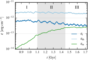
Figure 1: The average thermal, turbulent kinetic and magnetic energy densities, respectively $\epsilon_{\rm th}$, $\epsilon_{\rm t}$ and $\epsilon_{\rm m}$, within the simulation domain. Various stages of the magnetic field evolution are marked with numbers at the top of the frame and separated with shading in Stage II. During Stage I the magnetic field is dynamically insignificant so the evolution is essentially hydrodynamic. Stage II is transitional, whereas the magnetic field has reached a statistically steady state and is dynamically important in Stage III.

With respect to the magnetic field properties, the simulated ISM evolves through three main stages during the time period under consideration (Fig. 1). Stage I is represented by 12 snapshots at $0.825\leq t\leq 1.100\,{\rm Gyr}$; here the magnetic field contribution to the total energy density is negligible and its strength grows exponentially in time, representative of the kinematic phase of a turbulent dynamo. Snapshots 13–25 cover Stage II, the transition from the kinematic dynamo to a statistically steady state of the magnetic field. Stage III, represented by the snapshots 26–37 at $1.450\leq t\leq 1.725\,{\rm Gyr}$, is the dynamo-saturated stage where the magnetic energy is comparable to the kinetic energy of the turbulent flow.

During the whole evolution, the thermal state of the system remains unchanged (thermal energy density, $\varepsilon_{\text{th}}\approx\text{const}$) but the kinetic energy density of the turbulent flow $\varepsilon_{\text{t}}$ decreases slightly as the dynamo grows and saturates. At the end of the simulation, the turbulent kinetic and magnetic energies are comparable; the mean gas number density within the box is approximately $0.24\,{\rm cm}^{-3}$, the typical turbulent flow speed is about $14\,{\rm km\,s^{-1}}$ and the magnetic field strength is close to $2.5\,\mu{\rm G}$.

2.1 Gas density fluctuations

The gas density $n(\textbf{{x}})$ is represented as the sum of the mean $\langle n\rangle$ and fluctuating (random) $\delta n$ parts, both functions of position. The mean density is obtained by Gaussian smoothing:

$$\langle n\rangle(\textbf{{x}})=\int_{V}n(\textbf{{x}}\arcmin)\,G_{l}(\textbf{{x}}-\textbf{{x}}^{\prime})\,\mathrm{d}^{3}\textbf{{x}}^{\prime}\,,\qquad\delta n(\textbf{{x}})=n-\langle n\rangle\,,$$ (1)

where $G_{l}(\textbf{{x}})=\left(2\pi l^{2}\right)^{-3/2}\exp\left[-|\textbf{{x}}|^{2}/(2l^{2})\right]$ is the Gaussian kernel, and $V$ denotes the volume of the computational domain. The averaging scale for this Gaussian smoothing operation, $l=50\,{\rm pc}$, was obtained by Gent et al. (2013a); this defines the kernel that maximises the difference between the scales of the averaged and fluctuating quantities in the power spectra (see also Section 2.2 of Hollins et al., 2017). The mean value of the fluctuations, $\langle\delta n\rangle$, is negligible at $z\neq 0$ and close to zero at $z=0$ where the density fluctuations are the strongest. The deviation of $\langle\delta n\rangle$ from zero is an unavoidable consequence of using Gaussian smoothing as the averaging procedure; Germano (1992) presents a consistent formalism for this and similar averaging methods.

We have also tested another averaging procedure where the mean gas density is defined as the horizontal average, $\langle n\rangle(z)=\iint_{z=\text{const}}n(\textbf{{x}})\,\mathrm{d}x\,\mathrm{d}y$. However, this leads to physically unacceptable values of the correlation length of the density fluctuations in excess of $200\,{\rm pc}$, whereas physically justifiable values (and those observed in the ISM) are about $100\,{\rm pc}$ or less. It is also worth noting that there is no need for the large-scale density to be perfectly uniform in $x$ and $y$ and only depend on $z$: the horizontal averaging disregards this fact (for details, see Gent et al., 2013a).

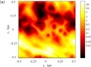
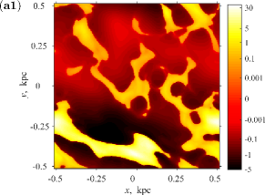
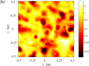
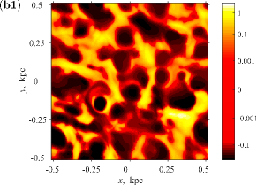
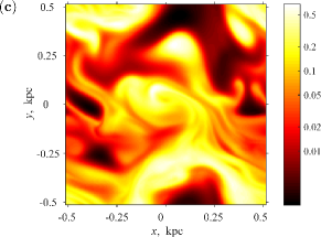
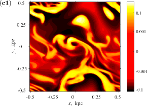
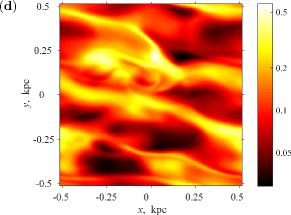
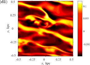
Figure 2: Examples of the gas density distribution $n(x,y)$ (left column) and density fluctuations $\delta n(x,y)$ (right column), both in cm^-3, (a) and (a1): $z=0$, $t=1\,{\rm Gyr}$, (b) and (b1): $z=0$, $t=1.6\,{\rm Gyr}$, (c) and (c1): $z=-0.5\,{\rm kpc}$, $t=1\,{\rm Gyr}$, and (d) and (d1): $z=-0.5\,{\rm kpc}$, $t=1.6\,{\rm Gyr}$.

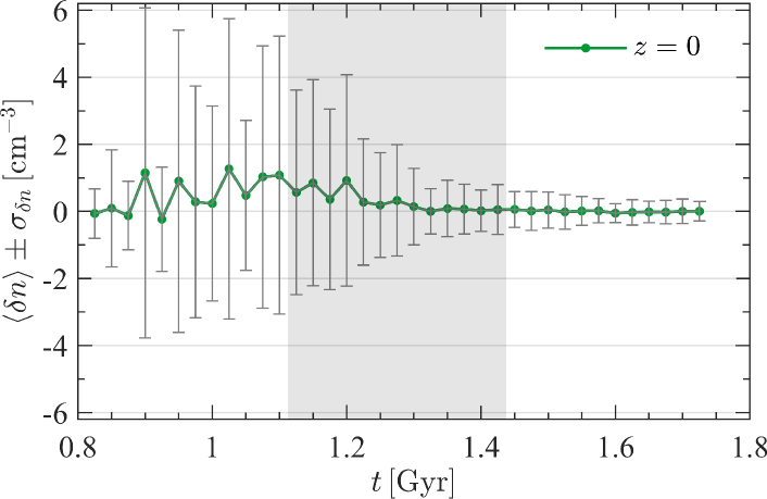
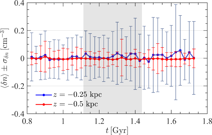
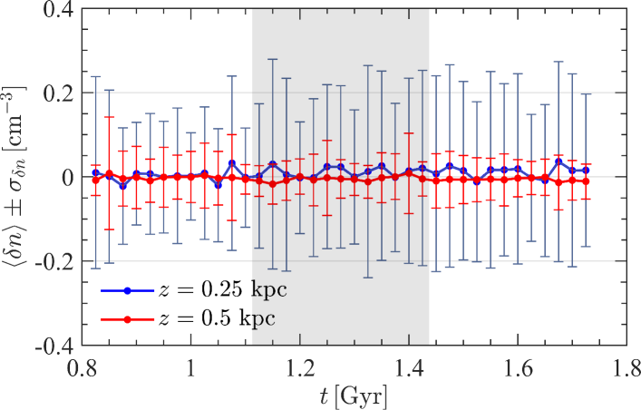
Figure 3: Time variation of the mean of the fluctuations of total gas density $\langle\delta n\rangle$ and its standard deviation $\sigma_{\delta n}$ for the values of $z$ specified in the legend. At later times, when the magnetic field is stronger, $\sigma_{\delta n}$ at $z=0$ decreases.

The system is stratified, so all physical quantities vary systematically with $z$. Therefore, we examined horizontal cross-sections of the gas density fluctuations at fixed $|z|=0,0.25$ and $0.5\,{\rm kpc}$. Examples of the gas density distribution and its fluctuations are shown in Fig. 2, using snapshots taken from Stages I (kinematic dynamo) and III (fully nonlinear dynamo). Comparison of Panels (a) and (b), and especially (a1) and (b1) shows that the strongly magnetised gas is more homogeneous, with the total, mean and fluctuating gas densities in the ranges $0\leq n\leq 37\,{\rm cm}^{-3}$, $0\leq\langle n\rangle\leq 8\,{\rm cm}^{-3}$ and $-7\leq\delta n\leq 31\,{\rm cm}^{-3}$ when the magnetic field is negligible as opposed to $0\leq n\leq 3.3\,{\rm cm}^{-3}$, $0.2\leq\langle n\rangle\leq 1.5\,{\rm cm}^{-3}$ and $-0.7\leq\delta n\leq 1.9\,{\rm cm}^{-3}$ when the magnetic field is strong. The horizontally averaged gas density at $z=0$ changes from $1.8$ to $0.6\,{\rm cm}^{-3}$ from Stage I to Stage III.

The supernova rate decreases exponentially with $|z|$, with a scale height of $90\,{\rm pc}$ (less frequent Type I supernovae have the scale height of $325\,{\rm pc}$). The numerous circular structures in Panels (a)–(b1) are supernova remnants, visible as holes in the gas distribution since gas in their interior is hot and rarefied. The cellular structure in Panels (b) and (b1), corresponding to a spongy structure in 3D, is more pronounced in the saturated phase than at earlier times, as shown in Panels (a) and (a1). This difference in the density fields, apparently associated with the magnetic field, can be detected by the naked eye at $z=0$ but not in Panels (c)–(d1) that show the gas distribution at $z=-500\,{\rm pc}$. At larger values of $|z|$, the gas is more homogeneous, with $0\leq n\leq 0.7\,{\rm cm}^{-3}$, $0\leq\langle n\rangle\leq 0.4\,{\rm cm}^{-3}$ and $-0.2\leq\delta n\leq 0.5\,{\rm cm}^{-3}$ in Panels (c) and (c1), and $0.03\leq n\leq 0.57\,{\rm cm}^{-3}$, $0.07\leq\langle n\rangle\leq 0.31\,{\rm cm}^{-3}$ and $-0.12\leq\delta n\leq 0.31\,{\rm cm}^{-3}$ in Panels (d) and (d1). By comparing scales, a reduction in the intensity of the fluctuations is evident, and large-scale gas structures extended at a small angle to the $x$-axis, produced by the large-scale magnetic field, are clearly visible in Panels (d) and (d1). Quantification of the small-scale gas structures is the purpose of this paper.

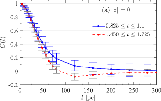
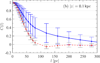
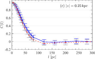
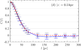
Figure 4: The auto-correlation functions of Eq. (2), in horizontal planes $z=\text{const}$, for the gas density fluctuations $\delta n$. These have been time-averaged over Stage I (solid, blue) and Stage III (dashed, red) at the values of $z$ specified in the legends. The error bars represent the standard deviation around the mean in each stage; the statistical errors of $C(l)$ are negligible.

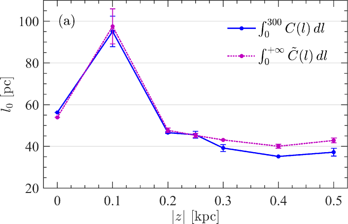
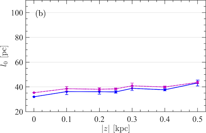
Figure 5: The correlation length $l_{0}$ from Eq. (3) as a function of $z$ in Stage I (upper panel; negligible magnetic field) and Stage III (lower panel; dynamically significant magnetic field). Shown are $l_{0}$ obtained from numerical integration of $C(l)$ over $0\leq l\leq 300\,{\rm pc}$ (solid, blue), analytical integration of $\tilde{C}(l)$ over $0\leq l<\infty$ (dotted, magenta), obtained from the time-averaged autocorrelation functions shown in Fig. 4.

Figure 3 shows variations with time of the mean value of the density fluctuations $\langle\delta n\rangle$ and its standard deviation $\sigma_{\delta n}$ at $z=0$, $\pm 0.25$ and $\pm 0.5\,{\rm kpc}$. The fluctuations have a non-vanishing mean value because the averaging is defined as Gaussian smoothing and it does not satisfy the Reynolds rules (Germano, 1992). Both the magnitude and the range of density fluctuations are larger in Stage I when the magnetic field is weak, and the variation with time is stronger at the mid-plane. However, the magnetic field reduces the fluctuations very significantly. This effect is hardly noticeable at $|z|=0.25$ and $0.5\,{\rm kpc}$ even though we will show that it is readily detectable with the topological data analysis in Section 5.

3 Correlation analysis

New methods of analysis rarely invalidate the established ones, and require careful justification of their advantages. Before using topological data analysis, we conduct a standard correlation analysis of the gas density field, not only to extract the information it can provide, but also to identify its limitations. Correlation analysis of the gas density, speed and magnetic field in these simulations is provided by Hollins et al. (2017). Here we present a more detailed analysis of the gas density fluctuations.

3.1 Autocorrelation function of gas density

For a stationary random field $f(\textbf{{x}})$, with $\textbf{{x}}=(x,y,z)$, the normalised auto-correlation function at a given height $z$ is defined by

$$C(l)=\sigma_{f}^{-2}\iint_{z=\text{const}}\left[f(\textbf{{x}})-\langle f\rangle\right]\left[f(\textbf{{x}}+\textbf{{l}})-\langle f\rangle\right]\,\mathrm{d}x\,\mathrm{d}y\,,$$ (2)

where $\sigma_{f}$ is the standard deviation of $f$, the lag $\textbf{{l}}=(l_{x},l_{y},0)$ is confined to the plane $z=\text{const}$ (over which the integral is evaluated), $l=|\textbf{{l}}|$, and $\langle f\rangle$ is given by Eq. (1). The auto-correlation function is further averaged over time in each of Stages I, II and III. Formally, we should write $C(l,z)$ here, to indicate that the auto-correlation function depends on $z$. However, we only ever consider the $l$ dependence of this function at fixed $z$, so we have abbreviated this for notational convenience.

The results are shown in Fig. 4 for Stage I (solid, blue) and Stage III (dashed, red) at $|z|=0,100,250$ and $500\,{\rm pc}$. The gas distribution is symmetric about the mid-plane $z=0$ on average. However, the size of the computational domain is relatively small, so that deviations from perfect symmetry in individual snapshots can be considerable. To verify that this does not affect our conclusions, we first plotted $C(l)$ separately for $z=250\,{\rm pc}$ and $z=-250\,{\rm pc}$ and similarly for $z=\pm 500\,{\rm pc}$. Indeed, the autocorrelation functions turned out to be symmetric with respect to $z=0$. As $C(l)$ at positive and negative values of $z$ are close to each other, we show the averaged correlation functions for $|z|=\text{const}$ in Fig. 4.

The difference between the autocorrelation functions obtained with and without a strong magnetic field (Stages I and III, respectively) is significant only at $z=0$ and $\pm 0.1\,{\rm kpc}$, shown in Panels (a) and (b) respectively, but even then the magnetic field does not lead to any characteristic features that could be used to unambiguously confirm its presence. For example, a negative tail of $C(l)$ develops at $z=0$ only in Stage III and could be thought to be a consequence of the magnetic field. However, at $|z|=500\,{\rm pc}$ a similar (albeit weaker) negative tail is stronger in Stage I. We also found that in Stage I the autocorrelation function at $|z|=100\,{\rm pc}$ significantly differs from that at other $z$: the correlation function in Stage I decreases with $l$ slower than at other values of $|z|$, with larger scatter between the snapshots reflected in longer error bars, and the change between Stages I and III is stronger. This is apparently related to the fact that supernova activity reduces significantly beyond $|z|\simeq 100\,{\rm pc}$. However, the autocorrelation function has a similar form at all distances from the mid-plane in Stage III, presumably because magnetic pressure redistributes gas along $|z|$, reducing the significance of the supernova layer.

As discussed by Evirgen et al. (2017a), the magnetic field is strongest at $|z|=200\text{--}300\,{\rm pc}$, so its effects on the gas distribution can be expected to be most pronounced there. However, the autocorrelation functions do not show any signs of this.

3.2 Correlation length

The correlation length is defined as

$$l_{0}=\int_{0}^{\infty}C(l)\,\mathrm{d}l\,.$$ (3)

Calculation of $l_{0}$ from experimental or numerical data that is restricted to a relatively narrow range of $l$ requires some caution. For example, integration of $C(l)=\exp(-l/l_{0})$ to $l=L$ leads to a relative error of $\exp(-L/l_{0})$ in the correlation length, about five per cent for $L=3l_{0}$. The problem can be aggravated by statistical errors in $C(l)$. As suggested by Hollins et al. (2017), as well as integrating $C(l)$ numerically within the range $0\leq l\leq 300\,{\rm pc}$, we approximated the derived autocorrelation functions as

$$\tilde{C}(l)=\cos\left(al^{2}+bl\right)\,\exp\left[-l^{2}/(2c^{2})\right]\,,$$ (4)

and obtained $a$, $b$ and $c$ from least-squares fits to the autocorrelation functions of Section 3.1. The unweighted fits were used, and the fit quality was verified; the $\chi^{2}$ was test satisfied for all of the fits. This analytic approximation was then integrated over $0\leq l<\infty$. The term $\cos\left(al^{2}+bl\right)$ is required to allow for the negative values of $C(l)$ at $|z|\ga 100\,{\rm pc}$ (see Fig. 4). Another property of a correlation function is its curvature at $l=0$, usually characterised in terms of the Taylor micro-scale, $\lambda$, defined via (Tennekes & Lumley, 1972)

$$C(l)\approx 1-(l/\lambda)^{2}\qquad\text{for }l/\lambda\ll 1\,.$$ (5)

However this a more difficult quantity to measure than the correlation length, because it is determined by correlations at small-scales, which can be influenced by the grid resolution. For similar reasons, differences in the small-scale structures in these simulations are difficult to characterise using only a correlation analysis.

Table 1: Summary of notation.

Symbol	Meaning	Reference
$l_{0}$	Correlation length	Section 3
$\lambda$	Taylor microscale	Section 3
$h$	The level of an isocontour or isosurface	Section 4
$\beta_{0}$	A number of components of a sublevel set at a level $h$	Section 4
$\beta_{1}$	A number of holes of a sublevel set at a level $h$	Section 4
$B_{0}$	The total number of components in a filtration, equal to the number of points in the $\beta_{0}$ persistence diagram	Section 4
$B_{1}$	The total number of holes in a filtration, equal to the number of points in the $\beta_{1}$ persistence diagram	Section 4
$\tilde{\beta}_{0}$	A number of components of a sublevel set at a level $h$ per area of $l_{0}^{2}$	Section 4
$\tilde{\beta}_{1}$	A number of holes of a sublevel set at a level $h$ per area of $l_{0}^{2}$	Section 4
$\widetilde{B}_{0}$, $\widetilde{B}_{1}$	The total number of components and holes in a filtration per correlation cell	Section 5
$\chi$	Euler characteristic, in 2D: $\beta_{0}-\beta_{1}$; per correlation length $\widetilde{B}_{0}-\widetilde{B}_{1}$	Section 5

Figure 5 shows the $z$-dependence of the correlation length, obtained as described in the figure caption. The estimates of $l_{0}$ at positive and negative values of $z$ are very close to each other, so we present the average values. It is clear from the comparison of the upper and lower panels of Fig. 5 that magnetic fields significantly affect the statistics of the gas distribution in the region $|z|\la 300\,{\rm pc}$, with significant differences in the corresponding correlation lengths between Stages I and III. Further from the mid-plane, the correlation lengths do not change appreciably with time.

4 Topological data analysis

Unlike correlation analysis, topological data analysis is not restricted to finite-order statistical moments of a random field. Its aim, achieved through topological filtration, is to isolate significant properties of a random field that can be used to simplify it and thus to make it amenable to analysis, comparison and statistical inference. Rigorous definitions of the Betti numbers and related concepts can be found in Adler et al. (2010); Edelsbrunner & Harer (2010); Adler & Taylor (2011) and Edelsbrunner (2014) while Park et al. (2013) and Pranav et al. (2017) provide useful and less formal expositions. Here we briefly present the basics at an intuitive level.

Betti numbers $\beta_{n}$ characterise the topological structures that form a random field $f(\textbf{{x}})$. Firstly, an isosurface at $f(\textbf{{x}})=h$, where $h$ is a constant, of a 3D random field is defined The topology of the isosurface is then characterised in terms of isolated components, loops and closed shells (known as cycles of dimension 0, 1 and 2, respectively). The Betti numbers quantify this structure: $\beta_{0}$ is the number of components, $\beta_{1}$ is the number of loops that cannot be reduced to a point by a continuous deformation. The Betti numbers are topological invariants, i.e. they are not affected by translations, rotations and continuous deformations of the random field. In a typical astrophysical application, the components represent matter clumps or clouds, the cycles are closed chains of matter and the shells surround regions of reduced density (voids).

Representation of the random field in terms of the Betti numbers, and their variation as the level $h$ of the isosurface changes, is called the filtration of the random field: it isolates topologically significant features of the field, and thus facilitates their analysis and comparison. For a given $h$, the superlevel and sublevel sets are defined to be the sets of points x where $f(\textbf{{x}})>h$ or $f(\textbf{{x}})<h$ respectively. Topological filtration is therefore a collection of topologically distinct superlevel or sublevel sets of a random field, similar to those shown in Figs. 6a and 6b. The topology of such a set only changes when the level $h$ passes through a critical point of the random field. Therefore, a filtration of the random field only contains topologically significant information about it. The topology of the superlevel or sublevel sets is characterised in terms of the Betti numbers, $\beta_{n}$.

In this paper we will also use the number of components or holes for the whole filtration (i.e. the total numbers obtained for all levels $h$), which is equal to the total number of components and holes at all levels $h$. These two quantities, related to the Betti numbers $\beta_{0}$ and $\beta_{1}$, are denoted as $B_{0}$ and $B_{1}$, respectively. Those topological features of the isosurfaces that occur continuously over a wide range of isosurface levels are said to be persistent and considered to be the most important. In the next section we discuss in more detail the idea of topological filtration and Betti numbers and then illustrate them using a specific example in Section 4.2. Some readers may find it useful to read Section 4.2 in conjunction with or even before Section 4.1. For later convenience, the key notation is presented in Table 1; the section where each notation appears in the text for the first time is shown in the right column.

4.1 Topological filtration and Betti numbers

The above description refers to a three-dimensional random field. In two dimensions, only the Betti numbers $\beta_{0}$ and $\beta_{1}$ are defined. To illustrate the technique, consider a continuous random function $f(x,y)$ defined in a finite domain, and its isocontour of a level $h$, i.e. a curve in the $(x,y)$-plane where $f=h$. The set of points $(x,y)$ where $f>h$ is therefore the superlevel set; its complement, $f<h$, is the sublevel set. To filter out insignificant noise but allow the important elements of $f$ to pass through the filter, we vary $h$ from smaller to larger values and record the number of components (clouds) and holes in each isocontour together with the values of $h$ where components and holes appear and disappear. The isocontours can also be scanned down from larger to smaller values of $h$: this does not affect the results. The transition from the sublevel sets to superlevel sets swaps the persistent diagrams of $\beta_{0}$ and $\beta_{1}$ (in 2D). Here we use the sublevel sets, i.e. scan $f(x,y)$ up from smaller to larger values.

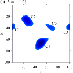
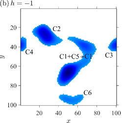
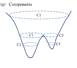
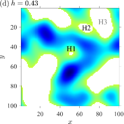
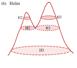
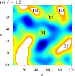
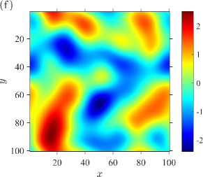
Figure 6: Topological filtration of a continuous, smooth, 2D Gaussian scalar field, $f(x,y)$, which has a vanishing mean value, unit standard deviation, and an auto-correlation function $C(l)=\exp\left[-l^{2}/(2L^{2})\right]$, where $L\approx 15$. The colour table, which is defined by the colour bar shown near Panel (f), shows the spatial variations of this scalar field. Sublevel sets, i.e. regions where $f(x,y)<h$, are shown for increasing values of $h$: (a) $h=-1.25$, (b) $h=-1$ (c) $h=0.4$, (d) $h=0.43$ and (e) $h=1.2$. The components (C) and holes (H) are labelled in Panels (a), (b), (c), (d) and (e) as described in the text. Panels (g) and (h) show how the components merge and the holes split as the level $h$ changes. Panel (f) presents the full range of $f(x,y)$.

When the level $h$ reaches the lowest value of $f$ in the domain, the first component emerges as illustrated in Fig. 6. Each local minimum of $f$ adds a new component when it is reached by the increasing isocontour level $h$. Two (or more) components can merge, when $h$ increases, if they are connected by a gorge (where a saddle point should be located); then the labelling convention is that the younger component (i.e., that formed at a larger $h$) dies whereas the older one continues to exist. Two components merge when the isocontour contains a saddle point, see Fig. 6, panel (g); three components merge, when $h$ passes through a monkey saddle (a degenerate critical point with a local minimum along one direction and inflection point in another, as opposed to the ordinary saddle with a minimum in one direction an maximum in another). Three (or more) components can merge, when there are three (or more) saddle points at the same level $h$.

The components can merge to form a loop whose interior is a hole; each hole at a level $h$ surrounds a local maximum of $f$ that will occur at some higher level. Holes are born when a loop is formed and die when $h$ passes through the corresponding local maximum of $f$. Holes can split up at a saddle point, in which case the labelling convention is to ascribe the original birth time to the hole with the larger eventual local maximum, and deem the current level to be the birth time of the second hole. Fig. 6, panel (h), illustrates this.

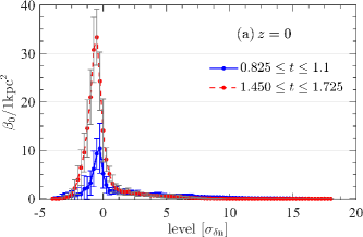
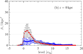
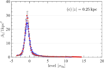
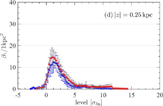
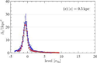
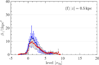
Figure 7: The dependence of the Betti numbers per unit area, $\beta_{0}$ in the left-hand column and $\beta_{1}$ on the right, of the gas density fluctuations at a level $h$ (specified in the units of $\sigma_{\delta n}$, the standard deviation of the density fluctuations). These are plotted at various distances from the mid-plane $z=0$ as given in the legends, in Stage I (blue) and Stage III (red). Error bars represent the standard deviation of the scatter of data points between the snapshots involved in the time averaging. The difference between Stages I and III is significant only at $z=0$.

It is then clear that the birth and death of components and holes is intrinsically related to the nature of, and connections between, the stationary points of the random field (its extrema and saddles) and to the values of $f$ at those points. Betti numbers contain rich information about the random function. Eventually, as $h$ approaches the absolute maximum of $f$ in the domain, only one, most persistent component remains (and no holes). Therefore $\beta_{0}=1$ and $\beta_{1}=0$ at levels $h$ exceeding the absolute maximum of $f$ in the domain. The ‘lifetime’, or persistence of a component or a hole is characterised by the range of $h$ where it exists. Selecting only those features that are more persistent, one distils a simplified (and therefore, better manageable) topological portrait of the random field.

4.2 Illustrative example

The topological filtration of the scalar Gaussian random field that is illustrated in Fig. 6 has already been referred to in the previous discussion. Here we discuss this filtration in more detail, describing how the Betti numbers can be calculated. Panel (f) represents a realisation of a 2D Gaussian random field $f(x,y)$ whose absolute minimum, $f=-2.4$, occurs at $(x,y)=(50,35)$. Thus, the first component C1 is born at $h=-2.4$ and there are no holes at this level: we have $\beta_{0}=1$ and $\beta_{1}=0$ at $h=-2.4$. As $h$ increases, more components are born. At $h=-1.25$, Panel (a), there are five components C1–C5 and no holes: $\beta_{0}=5$ and $\beta_{1}=0$. At $h=-1$, Panel (b), component C6 has appeared, whereas C1 and C5 have merged via a saddle point between them, passed through at a smaller $h$; the surviving component is labelled C1 whereas C5 has died as it was born later than C1. There are no holes at $h=-1$: $\beta_{0}=5$ and $\beta_{1}=0$. At a higher level $h=0.4$, shown in Panel (c), most of the components are merged into a big island, and there is one more small island in the left bottom corner of the panel; moreover, one hole H1 appeared: $\beta_{0}=2$, $\beta_{1}=1$. We have indicated on this sketch where H3 will appear as the level is raised (it is not yet defined as a hole because it is not yet bounded). At a level $h=0.43$, Panel (d), the number of components is the same as in the previous panel, $\beta_{0}=2$. One more hole H2 has appeared, $\beta_{1}=2$. At a higher level $h=1.2$, Panel (e), all components have merged into a single island, $\beta_{0}=1$. There are three holes labelled H3–H5, each around a local maximum of $f$, so $\beta_{1}=3$. Note again that some holes (bordering on the field frame) have not yet completely formed and are not taken into account as holes. There are two such cases in panel (e). The holes H1 and H2, that surround the maxima lower than $f=1.2$, have already died (contracted).

4.3 Application to the ISM simulation

These ideas can be applied directly to the numerical simulation. The Betti numbers were computed using the algorithm suggested in Edelsbrunner & Harer (2010). The description of the algorithm can be also found in Makarenko et al. (2014). To represent the result of topological filtration of the field one can plot the number of components $\beta_{0}$ and the number of holes $\beta_{1}$ as a function of level $h$. Then, for a 2D field we obtain two curves, one for the components and one for the holes, showing changes that take place in the field structure. The Betti numbers obtained from scanning the gas density fluctuations in planes $z=\text{const}$ from smaller to larger values of $\delta n$ are shown in Fig. 7 as functions of the isocontour level $h$. Apart from at the mid-plane, $z=0$, the difference between Stages I and III is insignificant and can hardly be used for diagnostic purposes. As we discuss in Section 5, a more detailed analysis is required to reveal the differences.

4.4 Persistence diagrams

Returning to our illustrative example, having specified the structure and connections of the stationary points of $f$ in terms of the Betti numbers, $\beta_{0}$ and $\beta_{1}$, at various levels $h$, we turn to the persistence of each structural feature. Let $u$ be a level at which a component or a hole appears (is born) and $v$ a level where it disappears (dies). Apart from the list of features at each level $h$, the filtration described above results in the lists of $(u,v)$ pairs for both the components and the holes. The lifetime of each topological feature is defined as $v-u$. The longer the lifetime, the more prominent (persistent) is the feature. Since we are interested in the $h$-dependent connections between the features, which do not change if $f$ is continuously deformed (and thus represent topological invariants), the positions of the features in the $(x,y)$-plane are of no interest.

The pairs $(u,v)$ can be represented as points in the $(u,v)$-plane to obtain a persistence diagram. Then, filtration of a 2D field results in two persistence diagrams, one for each Betti number. As mentioned above, the total number of components and holes obtained from the filtration as the level $h$ changes from the lowest minimum to the highest maximum of the field, are referred to as $B_{0}$ and $B_{1}$ in this paper (see Table 1).

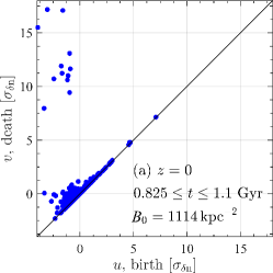
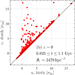
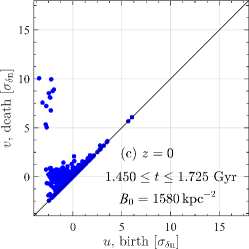
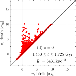
Figure 8: Persistence diagrams of the gas density fluctuations from all snapshots at $z=0$ for the components (left-hand panels, blue) and holes (right-hand panels, red) in (a)–(b) Stage I and (c)–(d) Stage III. Twelve persistence diagrams for each of Stage I and Stage III have been combined for each Betti number.

Figure 8 shows persistence diagrams for the gas density fluctuations $\delta n$ in all snapshots from Stage I (upper row) and Stage III (lower row) at $z=0$. Points at the largest distance from the diagonal represent the most stable, persistent features that have larger span in $\delta n$. The diagrams for both $B_{0}$ and $B_{1}$ are more compact in both $u$ and $v$ in Stage III reflecting a narrower range of the gas density fluctuations, i.e. a more homogeneous medium. In both stages, there is a relatively small number of very persistent components (points with large $v$ in the $B_{0}$ diagram), whereas the persistence of holes ($B_{1}$) is less extreme. On the other hand, the number of structures, either components ($B_{0}$) or holes ($B_{1}$), is larger by about 40 per cent in Stage III. This suggests a more structured gas distribution. Points at the bottom left corners of each diagram correspond to weak fluctuations at the lowest values of $\delta n$. Most components have $u,v<0$, indicative of numerous local minima in the gas density distribution since the filtration proceeds from smaller to larger values of $\delta n$. On the other hand, holes ($B_{1}$) occur mostly at $u,v>0$, representing cavities in a relatively dense gas.

4.5 Normalisation of Betti numbers

For a statistically stationary random field in 2D (or 3D), the magnitudes of the Betti numbers are proportional to the area (or volume) sampled, and they are therefore often presented per unit area (or volume). Park et al. (2013), Pranav (2015), Pranav et al. (2017), Sousbie (2011) and Sousbie et al. (2011) discuss Betti numbers per cubic pixel of Mpc³. With such a normalisation, the result would change if the random field was rescaled spatially, $\textbf{{x}}\to a\textbf{{x}}$ with $a=\text{const}$, despite the fact that its statistical properties remained essentially unchanged. Of course, the normalisation volume should change correspondingly, but this would not happen when the normalisation volume is chosen arbitrarily or when the observational or computational region is fixed in size. To allow for such trivial differences in random fields, the Betti numbers should be normalised to a physically significant volume (or area in 2D), leading to a dimensionless quantity.

For a random field, an obvious inherent spatial scale is the correlation length $l_{0}$, so the normalisation volume or area can be chosen as $l_{0}^{3}$ or $l_{0}^{2}$ in 3D or 2D, respectively (in the isotropic case). To provide a relevant context, we note that the number of local maxima or minima of a 2D Gaussian, isotropic random field per the correlation cell area $l_{0}^{2}$ follows from Longuet-Higgins (1957a, b) as

$$N_{0}=\frac{l_{0}^{2}}{6\pi\sqrt{3}}\left.\frac{\mathrm{d}^{4}C(l)/\mathrm{d}l^{4}}{-\mathrm{d}^{2}C(l)/\mathrm{d}l^{2}}\right|_{l=0}=\frac{\sqrt{3}}{12}\approx 0.14\,,$$ (6)

for the correlation function $C(l)=\exp[-\pi l^{2}/(4l_{0}^{2})]$ (for a discussion in terms of the autocorrelation function, see section 30 of Sveshnikov, 1966). It is also worth noting that the probabilistic properties of the local extrema of a Gaussian random field are controlled by the form of the autocorrelation function at small values of $l$, so the Taylor micro-scale $\lambda$ (see Eq. 5) is another natural normalisation lengthscale to consider. We tried using $\lambda^{2}$ for normalisation but found it less discriminating than $l_{0}^{2}$, probably due to the difficulties in its accurate determination, as mentioned in Sect. 3.2.

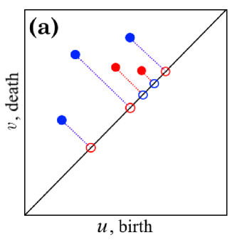
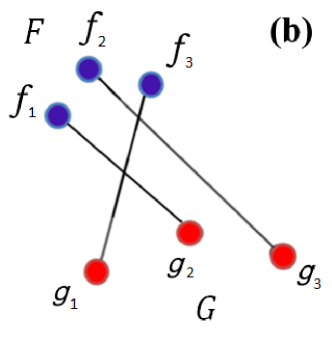
Figure 9: Illustration of the definition of the bottleneck distance, (a): adding points on a diagonal of the persistence diagram, (b): one of the possible matchings between two sets of points.

4.6 The bottleneck distance between persistence diagrams

Topological filtration produces persistence diagrams for the Betti numbers, i.e. sets of points in the $(u,v)$-plane shown in Fig. 8. Comparison of random fields then requires a quantification of differences between such clouds of points, i.e. the introduction of a measure in the space of persistence diagrams. One such measure is the bottleneck distance (Edelsbrunner & Harer, 2010; Edelsbrunner, 2014) often used to compare persistence diagrams in the exploration and development of various TDA techniques. We first present a formal definition of the bottleneck distance and then explain it with an example.

Consider two persistence diagrams $\mathbb{F}$ and $\mathbb{G}$, i.e. two sets of points in the $(u,v)$-plane. The bottleneck distance between two diagrams is

$$D(\mathbb{F},\mathbb{G})=\inf_{\mu:\,\mathbb{F}\to\mathbb{G}}\sup_{\textbf{{x}}\in\mathbb{F}}\left\|\textbf{{x}}-\mu(\textbf{{x}})\right\|_{\infty},$$

where $\mu:\,\mathbb{F}\to\mathbb{G}$ is a bijection, the infimum is over all bijections from $\mathbb{F}$ to $\mathbb{G}$, and a distance between points $\textbf{{x}}=(u_{\mathbb{F}},v_{\mathbb{F}})$ and $\textbf{{y}}=(u_{\mathbb{G}},v_{\mathbb{G}})$ is measured as $\left\|\textbf{{x}}-\textbf{{y}}\right\|_{\infty}=\max\{|u_{\mathbb{F}}-u_{\mathbb{G}}|,|v_{\mathbb{F}}-v_{\mathbb{G}}|\}$.

To clarify the definition of the bottleneck distance, consider how it is evaluated in practice for two persistence diagrams, $\mathbb{F}$ and $\mathbb{G}$, i.e. two sets of points in the $(u,v)$-plane shown in solid blue and red in Fig. 9. The bottleneck distance between them can be measured only if they contain the same number of points. Since two persistence diagrams can have different number of points, the diagrams are augmented as follows. We find the orthogonal projections of all points of $\mathbb{F}$ on the diagonal $u=v$ (red circles) and add them to the diagram $\mathbb{G}$ to obtain the set $G$ shown in Fig. 9a. Then we add the projections of all points of $\mathbb{G}$ (blue circles) to the diagram $\mathbb{F}$ to obtain the set $F$. Now $F$ and $G$ have the same size.

Consider all possible one-to-one matchings (or correspondences, bijections) between the sets $F$ and $G$. Suppose that there are $k$ such matchings. For example, for the configuration of points in Fig. 9b, there are 6 such matchings ($k=6$):

($$\textbf{{f}}_{1}$$ ), ( ), ( ),

( ), ( ), ( ),

( ), ( ), ( ),

( ), ( ), ( ),

( ), ( ), ( ),

( ), ( ), ( ).

Each pair of points (denoted $\textbf{{f}}_{j}$ and $\textbf{{g}}_{j}$) in a given matching has a cost defined as a geometric distance between them in the $(u,v)$-plane, denoted $|\textbf{{f}}_{j},\,\textbf{{g}}_{j}|=[(u_{fj}-u_{gj})^{2}+(v_{fj}-v_{gj})^{2}]^{1/2}$. If both points are at the diagonal, the cost of this pair is zero. The largest cost in a given matching is then introduced as

$$d_{k}=\max_{j}{|\textbf{{f}}_{j},\,\textbf{{g}}_{j}|},\qquad\textbf{{f}}_{j}\in F,\qquad\textbf{{g}}_{j}\in G,$$

where $k$ enumerates individual matchings of the sets $F$ and $G$. Having quantified all possible matchings between $F$ and $G$, the largest cost in each matching is recorded and its minimum value among all matchings is called the bottleneck distance between $F$ and $G$:

$$D(F,G)=\min_{k}d_{k}.$$

Details of algorithms for computation of the bottleneck distance can be found in Kerber et al. (2016). We used the software package dipha at https://github.com/DIPHA/dipha.

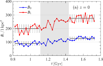
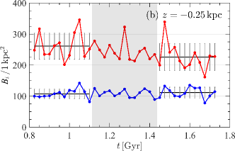
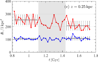
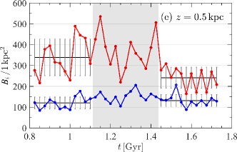
Figure 10: Evolution of the Betti numbers $B_{0}$ (blue) and $B_{1}$ (red) per $1\,{\rm kpc}^{2}$ at various distances $z$ from the mid-plane. The shaded area corresponds to the transition between the kinematic dynamo regime of Stage I (with negligible magnetic field) to the magnetically steady state of Stage III (where the magnetic field contribution is dynamically significant). Error bars represent the standard deviation of individual values of $B_{0}$ and $B_{1}$ within a stage.

5 Betti numbers of the gas density fluctuations

To focus on topological properties of the fluctuations in the gas density distribution, it is useful to standardise them, i.e. to reduce them to zero mean and renormalise to the unit standard deviation. In the rest of the text, we therefore use the following standardised density fluctuations,

$$\delta\tilde{n}=\frac{\delta n-\langle n\rangle}{\sigma_{\delta n}}\,,$$ (7)

where $\sigma_{\delta n}$ is the standard deviation of $\delta n$.

Figure 10 and Table 2 show the Betti numbers $B_{0}$ and $B_{1}$ per $1\,{\rm kpc}^{2}$ as a function of time. Despite significant asymmetry of the gas distribution around $z=0$ in individual snapshots, the Betti numbers are rather symmetric, and thus capture the overall, time-averaged symmetry of the system with respect to $z=0$. It also clear that the Betti numbers reflect a change in the gas distribution apparently associated with the magnetic field. Since $B_{1}>B_{0}$ in all cases, the gas structure is cellular (‘spongy’), with numerous holes, apparently supernova remnants filled with dilute gas.

Table 2: The Betti numbers $B_{0}$ and $B_{1}$ (per $1\,{\rm kpc}^{2}$) of the gas density fluctuations averaged in Stages I and III at various values of $z$, the distance to the mid-plane of the computational domain. The standard deviations have been calculated between individual snapshots.

	$B_{0}\pm\sigma_{B_{0}}$ $[\text{kpc}^{-2}]$			$B_{1}\pm\sigma_{B_{1}}$ $[\text{kpc}^{-2}]$
$z\ [\text{pc}]$	Stage I	Stage III		Stage I	Stage III
$\phantom{-}0$	$\phantom{0}90\pm 15$	$127\pm 12$		$199\pm 30$	$275\pm 27$
$-250$	$108\pm 15$	$111\pm 17$		$261\pm 42$	$226\pm 44$
$\phantom{-}250$	$105\pm 9\phantom{0}$	$109\pm 15$		$253\pm 40$	$208\pm 36$
$-500$	$127\pm 29$	$106\pm 25$		$405\pm 76$	$242\pm 94$
$\phantom{-}500$	$121\pm 28$	$132\pm 28$		$339\pm 88$	$242\pm 50$

The Betti numbers of Table 2 and Fig. 10, denoted $B_{0}$ and $B_{1}$ are normalised to an area of $1\,{\rm kpc}^{2}$ whose size has no physical significance. Meanwhile, the spatial scale of the density fluctuations, controlled by the correlation length shown in Fig 5 and Table 3, changes with time and $z$ and differs between Stages I and III, especially at small $|z|$. In order to correct for the variation in the scale of the density fluctuations and isolate changes in their topological properties, we calculated Betti numbers normalised to the correlation cell area

$$\tilde{\beta}_{n}=\beta_{n}(l_{0}/L)^{2}\,,$$ (8)

where $L=1.086\,{\rm kpc}$ is the horizontal size of the computational domain. The corresponding values totalled over levels are denoted $\widetilde{B}_{n}$. They are presented in Fig. 11 and Table 3.

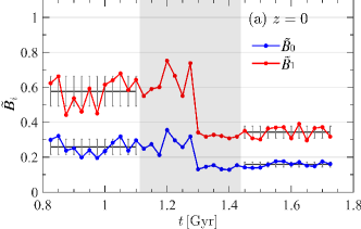
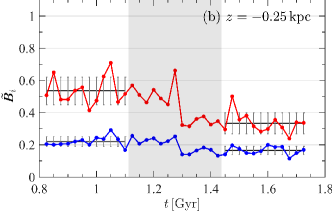
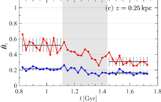
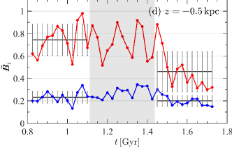
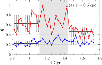
Figure 11: The Betti numbers per correlation area, $\widetilde{B}_{0}$ (blue) and $\widetilde{B}_{1}$ (red), as functions of time at various distances from the mid-plane in the same format as Fig. 10.

Table 3: The correlations lengths and totalled Betti numbers per correlation cell, $\widetilde{B}_{n}$ (with standard deviations within each stage), in Stages I and III at various $z$.

	$l_{0}$ [pc]			$\widetilde{B}_{0}\pm\sigma_{\widetilde{B}_{0}}$			$\widetilde{B}_{1}\pm\sigma_{\widetilde{B}_{1}}$
$z$ [pc]	Stage I	Stage III		Stage I	Stage III		Stage I	Stage III
$-$0	54	35		$0.26\pm 0.04$	$0.16\pm 0.02$		$0.58\pm 0.09$	$0.34\pm 0.03$
$-250$	45	38		$0.22\pm 0.03$	$0.17\pm 0.03$		$0.54\pm 0.09$	$0.33\pm 0.07$
$-$$250$	45	38		$0.22\pm 0.02$	$0.16\pm 0.02$		$0.52\pm 0.08$	$0.31\pm 0.05$
$-500$	43	44		$0.23\pm 0.05$	$0.20\pm 0.05$		$0.74\pm 0.14$	$0.46\pm 0.18$
$-$$500$	43	44		$0.22\pm 0.05$	$0.25\pm 0.05$		$0.62\pm 0.16$	$0.46\pm 0.10$

Table 4: The Euler characteristic $\chi$ and the Betti number ratios between Stages I and III, $r_{0}$ and $r_{1}$ of Eq. (9), normalised to the correlation cell area and presented at various distances to the mid-plane.

$z$ [pc]	$\chi$		$r_{0}$	$r_{1}$
	Stage I	Stage III
$\phantom{-25}0$	$-0.32\pm 0.10$	$-0.19\pm 0.04$	1.64	1.68
$-250$	$-0.31\pm 0.09$	$-0.17\pm 0.08$	1.34	1.60
$\phantom{-}250$	$-0.30\pm 0.08$	$-0.15\pm 0.05$	1.33	1.68
$-500$	$-0.51\pm 0.15$	$-0.26\pm 0.19$	1.16	1.62
$\phantom{-}500$	$-0.40\pm 0.17$	$-0.21\pm 0.11$	0.88	1.35

Remarkably, the evolution of the Betti numbers looks different when presented in terms of $\widetilde{B}_{n}$. The difference is especially pronounced at small $z$: while $B_{n}$ per kpc² increase from Stage I to Stage III at $z=0$, the $\widetilde{B}_{n}$ decrease. Trends at other values of $z$ shown in Figs. 10 and 11 are similar but the change in $\widetilde{B}_{1}$ between the stages is stronger in terms of the Betti numbers per correlation cell. The Betti numbers per correlation cell arguably have a clearer physical meaning and, conveniently, are dimensionless; we use them to draw physical conclusions from our results.

In all cases, $B_{1}>B_{0}$ independently of the normalisation. This inequality is consistent with a ‘spongy’ structure, where cavities of hot, rarefied gas produced by supernovae, contribute to $\beta_{1}$. Both Betti numbers per correlation cell decrease with magnetic field strength, and the change is most pronounced at smaller $|z|$. The reduction is stronger for the number of holes, $\widetilde{B}_{1}$. At large values of $|z|$, where the magnetic field is weaker (Evirgen et al., 2017b), the change in $\widetilde{B}_{n}$ between Stages I and III is weaker too. The only exception is the case of $\widetilde{B}_{0}$ at $z=0.5\,{\rm kpc}$ where the change is marginal.

Table 4 provides further diagnostics to justify our conclusions. Negative values of the Euler characteristic $\chi=\widetilde{B}_{0}-\widetilde{B}_{1}$ confirm the ‘spongy’ character of the density distribution with predominance of cavities. We also present the ratios of the Betti numbers in Stages I and III,

$$r_{0}=\frac{\left.\widetilde{B}_{0}\right|_{\rm Stage\ I}}{\left.\widetilde{B}_{0}\right|_{\rm Stage\ III}}\,,\qquad r_{1}=\frac{\left.\widetilde{B}_{1}\right|_{\rm Stage\ I}}{\left.\widetilde{B}_{1}\right|_{\rm Stage\ III}}\,.$$ (9)

Both ratios exceed unity at almost all $z$ (except for $r_{0}$ at $z=500\,{\rm pc}$) quantifying the reduction in the abundance of gas density features in Stage III as compared to Stage I, i.e. the homogenisation of the gas density distribution by the magnetic field. It is understandable that the ratios are smaller at $|z|=500\,{\rm pc}$ where the magnetic field is weaker. Away from the mid-plane, we observe $r_{1}>r_{0}$, so the effect of the magnetic field on gas cavities ($r_{1}$) is somewhat stronger than on density enhancements ($r_{0}$).

Table 5: The Mann–Whitney–Wilcoxon (MWW) and Kolomogorov–Smirnov (KS) statistical tests for the Betti numbers of individual snapshots from Stages I and III: they differ at the significance level of 95 per cent if the values of $p$ shown are less than 0.05. Entries corresponding to a significant difference are shown bold.

	MWW	KS		MWW	KS
$z$ [pc]	$B_{0}$ [kpc-2]			$\widetilde{B}_{0}$
$\phantom{-}0$	0.00004	0.00002		0.00004	0.000002
$-250$	0.49	0.79		0.0002	0.00002
$\phantom{-}250$	0.54	0.79		0.0002	0.00002
$-500$	0.09	0.07		0.14	0.19
$\phantom{-}500$	0.26	0.43		0.16	0.19

	MWW	KS		MWW	KS
$z$ [pc]	$B_{1}$ [kpc-2]			$\widetilde{B}_{1}$
$\phantom{-}0$	0.00004	0.000002		0.00004	0.000002
$-250$	0.03	0.07		0.0001	0.00002
$\phantom{-}250$	0.009	0.02		0.00006	0.00002
$-500$	0.0007	0.0002		0.001	0.0002
$\phantom{-}500$	0.007	0.02		0.02	0.02

We assess the statistical significance of the variations in Betti numbers using the Mann–Whitney–Wilcoxon and Kolomogorov–Smirnov tests, treating the totalled Betti numbers obtained for Stages I and III as samples from two distributions. Table 5 shows $p$-values for tests of whether Stages I and III have the same distributions. The difference in the distributions is significant at the 95 per cent confidence level when $p<0.05$. The two tests lead to similar conclusions with just one exception ($B_{1}$ at $z=-250\,{\rm pc}$). The difference between the Betti numbers of the gas density fluctuations between the states with and without strong magnetic field is statistically significant, and the Betti numbers per correlation cell provide more discriminatory power. The difference between Stages I and III is especially strong for the abundance of holes. The variation of the Betti numbers with the magnetic field strength suggests that the magnetic field strongly reduces the abundance of gas cavities.

Table 6: The mean values and standard deviations of the bottleneck distance $D$ (in cm^-3) between persistence diagrams (PD) for $B_{0}$ and $B_{1}$ at $z=0$ for snapshots within Stages I and III and between the stages (the upper part of the table) and at the earliest and latest times in Stages I and III, respectively (the lower part).

		Time interval	Number of	For $B_{0}$	For $B_{1}$
		[Gyr]	PD pairs	$\langle D\rangle\pm\sigma_{D}$ [cm-3]
All times	Within Stage I	0.275	66	$3.5\pm 2.3$	$3.8\pm 1.7$
	Within Stage III	0.275	66	$1.9\pm 1.2$	$2.6\pm 0.9$
	Between Stages I and III		144	$4.5\pm 2.7$	$4.0\pm 1.8$
Earliest and	Within Stage I	0.175	28	$3.5\pm 2.1$	$4.2\pm 1.8$
latest times	Within Stage III	0.175	28	$1.8\pm 1.0$	$2.5\pm 0.8$
	Between Stages I and III		64	$5.5\pm 2.7$	$4.5\pm 2.0$

Table 7: As Table 6 but separately for various distances to the mid-plane.

Quantity	Snapshots	Number of	$\langle D\rangle\pm\sigma_{D}$
		PD pairs	$z=0$	$z=-0.25\,{\rm kpc}$	$z=0.25\,{\rm kpc}$	$z=-0.5\,{\rm kpc}$	$z=0.5\,{\rm kpc}$
$B_{0}$	Within Stage I	$66$	$3.5\pm 2.3$	$2.7\pm 2.1$	$1.8\pm 1.0$	$1.4\pm 0.6$	$1.1\pm 0.4$
	Within Stage III	$66$	$1.9\pm 1.2$	$3.0\pm 2.3$	$2.1\pm 1.2$	$1.8\pm 1.0$	$1.9\pm 1.4$
	Between Stages I and III	$144$	$4.5\pm 2.7$	$3.0\pm 2.1$	$2.0\pm 1.3$	$1.6\pm 0.9$	$1.6\pm 1.2$
$B_{1}$	Within Stage I	$66$	$3.8\pm 1.7$	$2.4\pm 1.8$	$2.0\pm 0.9$	$1.8\pm 0.6$	$1.5\pm 0.5$
	Within Stage II	$66$	$2.6\pm 0.9$	$2.8\pm 1.9$	$2.0\pm 0.8$	$1.7\pm 0.7$	$2.1\pm 1.0$
	Between Stages I and III	$144$	$4.0\pm 1.8$	$2.9\pm 1.5$	$2.1\pm 0.9$	$1.7\pm 0.7$	$1.9\pm 1.0$

We calculated the bottleneck distances between each pair of persistence diagrams within Stages I and III as well as between the stages, and show the results in the upper part of Table 6. If the bottleneck distance is sensitive to the difference in the gas density distributions at early and late times, the inter-stage distance should be larger than the intra-stage distances. The mean values of $D$ conform to this expectation but the difference is less than one standard deviation. In an attempt to enhance the inter-stage differences, we treated in a similar manner the gas density from the earliest and latest periods of the simulation, when the difference between the magnetic field strengths is larger. The results, presented in the lower part of Table 6, show that the mean inter-stage bottleneck distance increases as expected but remains within one standard deviation despite that fact that the values of $\sigma_{D}$ remain similar to those in the larger samples. There still remains a possibility that the bottleneck distance is more useful at some distances to the mid-plane even if it is a poor diagnostic for the whole computational domain. A similar comparison of the intra-stage and inter-stage values of $D$ is presented in Table 7 for a selection of values of $z$. However, the results remain marginal.

Table 8: The Mann–Whitney–Wilcoxon (MWW) and Kolomogorov–Smirnov (KS) statistical tests for the bottleneck distances: $D$ in Stages I and III differ at the significance level of 95 per cent if the value of the probability shown is less than 0.05. Entries corresponding to a significant difference are shown bold.

	$z$ [pc]	MWW	KS
$B_{0}$	0	$\bf 0.0002$	$\bf 0.0002$
	$-250$	$0.27$	$0.29$
	$\phantom{-}250$	$0.29$	$0.54$
	$-500$	$\bf 0.05$	$0.09$
	$\phantom{-}500$	$\bf 0.02$	$\bf 0.0004$
$B_{1}$	0	$\bf 0.000003$	$\bf 0.0002$
	$-250$	$\bf 0.005$	$\bf 0.00002$
	$\phantom{-}250$	$\bf 0.006$	$\bf 0.004$
	$-500$	$0.16$	$0.20$
	$\phantom{-}500$	$\bf 0.0003$	$\bf 0.006$

The Mann–Whitney–Wilcoxon and Kolomogorov–Smirnov tests for the difference between the probability distributions of $D$ confirm the difference between the intra- and inter-stage bottleneck distances in some cases (Table 8) but the results remain mixed and unsystematic, especially for $B_{0}$. As discussed in Section 5, the effect of the magnetic field on $B_{1}$ is stronger, and statistical significance of this is reflected in the bottleneck distances for $B_{1}$. Nonetheless, the bottleneck distance proves to be a poor diagnostic of the difference between persistence diagrams of a realistic random field, as opposed to synthetic fields used in theoretical developments of the TDA. Henderson et al. (2017) show that the bottleneck distance also fails to distinguish persistence diagrams of non-Gaussian synthetic random fields.

6 Discussion and conclusions

We have shown that a magnetic field affects significantly the gas distribution in these ISM simulations. Topological data analysis of the gas density fluctuations reveals properties of interstellar turbulence that cannot be obtained from the correlation analysis. The magnetic field does not change the form of the autocorrelation function in such a way that it could be used as a diagnostic (e.g., producing local minima or maxima) for regions of strong magnetic fields (cf. Hollins et al., 2017). Magnetic effects do cause a significant reduction in the correlation length of the density fluctuations from $45\text{--}55\,{\rm pc}$ in Stage I of the simulations, where magnetic field is dynamically negligible, to $35\text{--}40\,{\rm pc}$ in Stage III where magnetic and turbulent energies are comparable. The change in the correlation length is restricted to the range $|z|\lesssim 300\,{\rm pc}$ of distances to the mid-plane where the magnetic field is strong. At larger values of $z$, the correlation length remains of order $40\,{\rm pc}$ throughout the simulation.

Our analysis focuses on the Betti numbers $\beta_{0}$ and $\beta_{1}$ of the gas fluctuations in two-dimensional slices through the three-dimensional computational domain. These Betti numbers quantify the number of isolated gas density structures ($\beta_{0}$) and holes in the gas distribution ($\beta_{1}$). Euler’s characteristic in two dimensions is the difference of the two Betti numbers, $\chi=\beta_{0}-\beta_{1}$. We suggest that the Betti numbers normalised to the size of the correlation cell, $\tilde{\beta}_{0}$ and $\tilde{\beta}_{1}$ defined in Eq. (8), and their total numbers in a filtration, $\widetilde{B}_{0}$ and $\widetilde{B}_{1}$, equal to the number of points in the corresponding persistence diagram, are physically informative and represent a better statistical diagnostic for topological differences of random fields.

The topological structure of the simulated ISM is characterised by a persistent inequality $\chi<0$, i.e. a higher abundance of cavities as compared to isolated gas clouds. As a crude estimate, the gas distribution contains one denser structure per five correlation cells of $40\text{--}50\,{\rm pc}$ in size (corresponding to $\widetilde{B}_{0}\simeq 0.2$) and one cavity per 1–2 correlation cell ($\widetilde{B}_{1}\simeq 0.6$) when the magnetic field is weak (Stage I). Since $\widetilde{B}_{0}<1$, the higher-density structures represent either large isotropic clouds, which is physically unlikely, or gas filaments spanning a few correlation cells. This suggests a spongy and yet filamentary structure dominated by elongated gas filaments and cavities filled with rarefied gas. The abundance of dense gas structures does not change much as the magnetic field grows but the abundance of cavities reduces to one per three correlation cells when the magnetic field becomes dynamically important (Stage III).

The reduction in both Betti numbers as the magnetic field grows suggests that it makes the gas distribution more homogeneous. A magnetic field of a few $\mu$G in strength can hardly affect expanding supernova remnants, so it is likely that it reduces the abundance of the hot, rarefied gas in old remnants or facilitates their merger with the ambient gas. Evirgen et al. (2017a) arrive at similar conclusions from their analysis of the fractional volume of the hot gas. Remarkably, the modification of the gas distribution by magnetic field is captured reliably even in a region at $|z|\ga 300\,{\rm pc}$ where the magnetic field is weaker and correlation analysis fails to detect any magnetic effects. So the topological methods applied here prove to be more sensitive to subtle differences between random fields than the traditional correlation analysis. Perhaps more importantly, topology reflects features of the random field that cannot be captured by traditional methods at all.

These methods of topological data analysis could also be applied productively to other ISM data which is expected to be non-Gaussian, both observed and simulated. Structured, often anisotropic gas density fluctuations emerge in simulations of molecular clouds, calling for methods of analysis more general than power spectra and low-order correlation functions. For example, Ballesteros-Paredes & Mac Low (2002) note that stronger driving of turbulence produces not only larger fluctuations about the mean density but also more extreme fluctuations (a greater proportion of the gas is at the highest densities). A shift of gas into the extremes in the density field can dominate the low-order statistical parameters of turbulence such as root-mean-square values. Magnetic fields can introduce further complications in the form of filamentary and anisotropic density structures. Such deviations from Gaussian statistical properties of velocity, density and magnetic field fluctuations are often described as intermittency. In such cases, Fourier spectra, with the associated random-phase approximation, and comparisons with simple models of turbulence (such as Kolmogorov’s or Burgers’ models) only provide necessary but not sufficient evidence of the relevance of the model. Moreover, compressibility (e.g., in shock-wave turbulence) and magnetic effects imprint nontrivial topological structure on turbulence in both molecular clouds and the diffuse interstellar medium. New methods of analysis are required that do not rely on the assumption of Gaussian statistics or weak deviations from it and are sensitive to morphological and topological properties of the random fields. For example, the nature of filamentary structures (Kalberla et al., 2016) prominent in both observations and many numerical simulations of interstellar gas requires reliable determination of their dimensions (see Makarenko et al., 2015; Kalberla et al., 2016, for examples of such analysis). The need for new methods of statistical comparison between theory and observations is discussed in an insightful review of Goodman (2011) and by Koch et al. (2017) who employ genus statistics, a topological measure earlier applied to the matter distribution in the cosmic web (Gott et al., 1987, and many later papers).

References

- Adler & Taylor (2011) Adler R., Taylor J. E., 2011, Topological Complexity of Smooth Random Functions: École D’Été de Probabilités de Saint-Flour XXXIX-2009. Springer, Berlin
- Adler et al. (2007) Adler R. J., Taylor J. E., Worsley K. J., 2007, Applications of Random Fields and Geometry: Foundations and Case Studies. http://citeseerx.ist.psu.edu/viewdoc/summary?doi=10.1.1.703.5392 (accessed April 30, 2017)
- Adler et al. (2010) Adler R. J., Bobrowski O., Borman M. S., Subag E., Weinberger S., 2010, Persistent homology for random fields and complexes. Inst. of Mathematical Statistics, Beachwood, Ohio, USA, pp 124–143
- Ballesteros-Paredes & Mac Low (2002) Ballesteros-Paredes J., Mac Low M.-M., 2002, ApJ, 570, 734
- Ballesteros-Paredes et al. (1999) Ballesteros-Paredes J., Vázquez-Semadeni E., Scalo J., 1999, ApJ, 515, 286
- Bendre et al. (2015) Bendre A., Gressel O., Elstner D., 2015, Astron. Nachr., 336, 991
- Brandenburg & Dobler (2002) Brandenburg A., Dobler W., 2002, Comput. Phys. Commun., 147, 471
- Brandenburg & Dobler (2010) Brandenburg A., Dobler W., 2010, Pencil: Finite-difference Code for Compressible Hydrodynamic Flows, Astrophysics Source Code Library (ascl:1010.060)
- Burkhart et al. (2012) Burkhart B., Lazarian A., Gaensler B. M., 2012, ApJ, 749, 145
- Carlsson (2009) Carlsson G., 2009, Bull. Am. Math. Soc., 46, 255
- Chepurnov et al. (2008) Chepurnov A., Gordon J., Lazarian A., Stanimirovic S., 2008, ApJ, 688, 1021
- Cramér & Leadbetter (2013) Cramér H., Leadbetter M. R., 2013, Stationary and related stochastic processes: Sample function properties and their applications. Dover, Mineola, NY
- De Avillez & Breitschwerdt (2004) De Avillez M. A., Breitschwerdt D., 2004, A&A, 425, 899
- De Avillez & Breitschwerdt (2012) De Avillez M. A., Breitschwerdt D., 2012, ApJ, 761, L19
- De Avillez et al. (2012) De Avillez M. A., Asgekar A., Breitschwerdt D., Spitoni E., 2012, MNRAS, 423, L107
- Edelsbrunner (2014) Edelsbrunner H., 2014, A Short Course in Computational Geometry and Topology. Springer, Berlin
- Edelsbrunner & Harer (2010) Edelsbrunner H., Harer J., 2010, Computational Topology: An Introduction. American Mathematical Society
- Elmegreen & Scalo (2004) Elmegreen B. G., Scalo J., 2004, ARA&A, 42, 211
- Evirgen et al. (2017a) Evirgen C. C., Gent F. A., Shukurov A., Fletcher A., Bushby P., 2017a, MNRAS (submitted)
- Evirgen et al. (2017b) Evirgen C. C., Gent F. A., Shukurov A., Fletcher A., Bushby P., 2017b, MNRAS, 464, L105
- Gent et al. (2013a) Gent F. A., Shukurov A., Sarson G. R., Fletcher A., Mantere M. J., 2013a, MNRAS, 430, L40
- Gent et al. (2013b) Gent F. A., Shukurov A., Fletcher A., Sarson G. R., Mantere M. J., 2013b, MNRAS, 432, 1396
- Germano (1992) Germano M., 1992, J. of Fluid Mech., 238, 325
- Goodman (2011) Goodman A. A., 2011, in Alves J., Elmegreen B. G., Girart J. M., Trimble V., eds, IAU Symposium Vol. 270, Computational Star Formation. pp 511–519 (arXiv:1107.2827), doi:10.1017/S1743921311000901
- Gott et al. (1987) Gott III J. R., Weinberg D. H., Melott A. L., 1987, ApJ, 319, 1
- Gressel et al. (2008) Gressel O., Elstner D., Ziegler U., Rüdiger G., 2008, A&A, 486, L35
- Henderson et al. (2017) Henderson R., Makarenko I., Bushby P., Fletcher A., Shukurov A., 2017, preprint, (arXiv:1703.07256)
- Henley et al. (2015) Henley D. B., Shelton R. L., Kwak K., Hill A. S., Mac Low M.-M., 2015, ApJ, 800, 102
- Hennebelle et al. (2008) Hennebelle P., Banerjee R., Vázquez-Semadeni E., Klessen R. S., Audit E., 2008, A&A, 486, L43
- Hennebelle et al. (2009) Hennebelle P., Mac Low M.-M., Vázquez-Semadeni E., 2009, Diffuse interstellar medium and the formation of molecular clouds. Cambridge University Press, Cambridge, p. 205
- Hill et al. (2012a) Hill A. S., Joung M. R., Mac Low M.-M., Benjamin R. A., Haffner L. M., Klingenberg C., Waagan K., 2012a, ApJ, 750, 104
- Hill et al. (2012b) Hill A. S., Joung M. R., Mac Low M.-M., Benjamin R. A., Haffner L. M., Klingenberg C., Waagan K., 2012b, ApJ, 761, 189
- Hollins et al. (2017) Hollins J. F., Sarson G. R., Shukurov A., Fletcher A., Gent F. A., 2017, preprint, (arXiv:1703.05187)
- Kalberla et al. (2016) Kalberla P. M. W., Kerp J., Haud U., Winkel B., Ben Bekhti N., Flöer L., Lenz D., 2016, ApJ, 821, 117
- Kerber et al. (2016) Kerber M., Morozov D., Nigmetov A., 2016, in Goodrich M., Mitzenmacher M., eds, Proceedings of the Eighteenth Workshop on Algorithm Engineering and Experiments (ALENEX). SIAM, Philadelphia, pp 103–112
- Kniazeva et al. (2015) Kniazeva I. S., Makarenko N. G., Urtiev F. A., 2015, Phys. Procedia, 74, 363
- Knyazeva et al. (2015) Knyazeva I. S., Makarenko N. G., Urtiev F. A., 2015, Geomagnetism and Aeronomy, 55, 1134
- Knyazeva et al. (2016) Knyazeva I. S., Makarenko N. G., Kuperin Y. A., Dmitrieva L. A., 2016, J. of Phys. Conf. Series, 675, 032028
- Koch et al. (2017) Koch E. W., Ward C. G., Offner S., Loeppky J. L., Rosolowsky E. W., 2017, MNRAS, 471, 1506
- Korpi et al. (1999a) Korpi M. J., Brandenburg A., Shukurov A., Tuominen I., 1999a, A&A, 350, 230
- Korpi et al. (1999b) Korpi M. J., Brandenburg A., Shukurov A., Tuominen I., Nordlund Å., 1999b, ApJ, 514, L99
- Kowal et al. (2007) Kowal G., Lazarian A., Beresnyak A., 2007, ApJ, 658, 423
- Leung et al. (2012) Leung T., Swaminathan N., Davidson P. A., 2012, J. of Fluid Mech., 710, 453
- Longuet-Higgins (1957a) Longuet-Higgins M. S., 1957a, Philos. Trans. of the R. Soc. Series A, 249, 321
- Longuet-Higgins (1957b) Longuet-Higgins M. S., 1957b, Philos. Trans. of the R. Soc. Series A, 250, 157
- Makarenko et al. (2007) Makarenko N. G., Karimova L. M., Novak M. M., 2007, Physica A, 380, 98
- Makarenko et al. (2014) Makarenko N. G., Malkova D. B., Machin M. L., Knyazeva I. S., Makarenko I. N., 2014, Fundam. Prikl. Mat. (Russian), translation in J. Math. Sci., 203, 806
- Makarenko et al. (2015) Makarenko I., Fletcher A., Shukurov A., 2015, MNRAS, 447, L55
- Makarenko et al. (2016) Makarenko N., Kalimoldayev M., Pak I., Yessenaliyeva A., 2016, Open Eng., 6, 44
- Orszag (1977) Orszag S. A., 1977, in Balian R., Peube J.-L., eds, Fluid Dynamics, Les Houches Summer School. Gordon and Breach, New York, pp 235–374
- Padoan et al. (2004) Padoan P., Jimenez R., Nordlund Å., Boldyrev S., 2004, Phys. Rev. Lett., 92, 191102
- Park et al. (2013) Park C., et al., 2013, J. of Korean Astron. Soc., 46, 125
- Piontek et al. (2009) Piontek R. A., Gressel O., Ziegler U., 2009, A&A, 499, 633
- Pranav (2015) Pranav P., 2015, Phd dissertation, University of Groningen, Johann Bernoulli Inst. for Math. and Computer Science
- Pranav et al. (2017) Pranav P., Edelsbrunner H., van de Weygaert R., Vegter G., Kerber M., Jones B. J. T., Wintraecken M., 2017, MNRAS, 465, 4281
- Sahni et al. (1998) Sahni V., Sathyaprakash B. S., Shandarin S. F., 1998, ApJ, 495, L5
- Scalo & Elmegreen (2004) Scalo J., Elmegreen B. G., 2004, ARA&A, 42, 275
- Schmalzing & Buchert (1997) Schmalzing J., Buchert T., 1997, ApJ, 482, L1
- Schmalzing et al. (1999) Schmalzing J., Buchert T., Melott A. L., Sahni V., Sathyaprakash B. S., Shandarin S. F., 1999, ApJ, 526, 568
- Shukurov et al. (2017) Shukurov A., Snodin A., Seta A., Bushby P., Wood T., 2017, ApJ, 839, L16
- Sousbie (2011) Sousbie T., 2011, MNRAS, 414, 350
- Sousbie et al. (2011) Sousbie T., Pichon C., Kawahara H., 2011, MNRAS, 414, 384
- Sveshnikov (1966) Sveshnikov A. A., 1966, Applied Methods of the Theory of Random Functions. Pergamon, Oxford
- Tennekes & Lumley (1972) Tennekes H., Lumley J. L., 1972, First Course in Turbulence. MIT Press, Cambridge
- Vázquez-Semadeni (2015) Vázquez-Semadeni E., 2015, in Lazarian A., de Gouveia Dal Pino E. M., Melioli C., eds, Magnetic Fields in Diffuse Media. Springer, Berlin, p. 401
- Wilkin et al. (2007) Wilkin S. L., Barenghi C. F., Shukurov A., 2007, Phys. Rev. Lett., 99, 134501
- Zeldovich et al. (1990) Zeldovich Y. B., Ruzmaikin A. A., Sokoloff D. D., 1990, The Almighty Chance. World Scientific, Singapore
- Zhdankin et al. (2015) Zhdankin V., Uzdensky D. A., Boldyrev S., 2015, ApJ, 811, 6
- Zhdankin et al. (2016) Zhdankin V., Boldyrev S., Uzdensky D. A., 2016, Phys. of Plasmas, 23, 055705