Proliferation of stability in phase and parameter spaces of nonlinear systems

Abstract

In this work we show how the composition of maps allows us to multiply, enlarge and move stable domains in phase and parameter spaces of discrete nonlinear systems. Using Hénon maps with distinct parameters we generate many identical copies of isoperiodic stable structures (ISSs) in the parameter space and attractors in phase space. The equivalence of the identical ISSs is checked by the largest Lyapunov exponent analysis and the multiplied basins of attraction become riddled. Our proliferation procedure should be applicable to any two-dimensional nonlinear system.

In high-dimensional dynamical systems the possibility of controlling the dynamics through parametric changes is of great interest. Adding a time dependent parameter it is possible to control the dynamics of the paradigmatic Hénon map generating multiply Isoperiodic Stable Structures (ISSs) on the parameter space and consequently increasing the number of attractors on the phase space. Numerical simulations and analytical results explain the origin of new stable domains due to saddle-node bifurcations for specific parametric combinations. The distance between the multiplied ISSs can be controlled by the intensity of the time dependent parameter and general rules for the occurrence of proliferation are treated in details. We believe that the present study represents a significantly new insight on the use of alternating forces to control the dynamics of complex nonlinear systems modeled by two-dimensional maps and can be extended to various applications ranging from physics, biology to engineering.

I Introduction

A huge number of physical systems in nature present regular or chaotic dynamics depending on parameters and initial conditions. We mention granular dynamics, coupled networks, brain dynamics, market crisis, chemical systems, laser physics, transport, extreme events, weather forecast, among many others. In nonlinear dynamics it is essential to know the correct parameter combination which leads to (or avoids) a specific dynamics. One crucial step for this was the discovery of structures in the parameter space of dynamical systems. Such structures, called Isoperiodic Stable Structures (ISSs), are Lyapunov stable islands in the parameter space, and are supposed to be generic in dynamical systems. For parameters chosen inside the ISSs the corresponding dynamics is stable and regular. ISSs were found in many systems, and we would like to mention some of them. In theoretical C. Cabeza et al. (2013) and experimental R.Stoop et al. (2010) electronic circuits, continuous systems Fraser and Kapral (1982); Broer et al. (1998); C. Bonatto et al. (2005); Zou et al. (2006); C. Bonatto and J. A. C. Gallas (2007); Medeiros et al. (2011); Gonchenko et al. (2013), maps Fraser and Kapral (1982); Markus and Hess (1989); Carcassés et al. (1991); J. A. C. Gallas (1993); Oliveira and Leonel (2011a, b); da Costa et al. (2016) lasers models Kovanis et al. (2010), cancer models M. R. Gallas et al. (2014), classical Celestino et al. (2011); A.Celestino et al. (2013); Manchein et al. (2013) and quantum ratchet systems G.G.Carlo (2012); M.W.Beims et al. (2015); Carlo et al. (2016). For the description of nature processes it is essential to discover generic properties for parameter combinations in nonlinear dynamical systems which can be applied to any realistic situation, independent of the specific physical system.

In this work we investigate the not trivial dynamics of the composition of two-dimensional discrete maps. We use the paradigmatic Hénon map (HM), whose relevant dynamics should be visible in any two-dimensional dissipative map. It is shown that composing HMs with distinct parameters, following a specific protocol, it is possible to generate multiple ISSs which can be split in the parameter space. Multioverlapping identical copies of the ISSs start to separate from each other with increasing intensity of the perturbative parameter $F$, enlarging the available stable domain in phase and parameter spaces. The generated overlapping ISSs are enlarged ISSs, found to be the factorized composition of identical copies of the original ISSs. The proposed method is generic and can be applied to ordinary problems involving nonlinear behaviors. Results for du-, tri-, sextu- and decuplications are described for the composition of Hénon maps with distinct parameters. Indications for the possible duplication of structures in parameter space was given for the composition of two quadratic coupled maps in the context of chaos suppression Loskutovy et al. (1996). The replication of a shrimp-like ISSs was observed in a continuous oscillator Medeiros et al. (2011), but its origin remained unknown. This work extends previous results for one-dimensional systems da Silva et al. (2017) to the non-trivial two-dimensional case.

The paper is presented as follows. In Sec. II we summarize the main properties observed in the one-dimensional case and in Sec. III the proliferation of shrimp-like ISSs in the parameter space of the two-dimensional Hénon map is presented. Section IV shows that multiple attractors are created in phase space with the corresponding riddled basin of attraction. In Sec. V we generalize our procedure showing the duplication of other more complicated ISSs and Sec. VI shows analytical results for the duplication of period $2$ (shortly written per-$2$) stability boundaries in parameter space. This corresponds to the duplication of ISSs. Section VII summarizes our results.

II Rules from The one-dimensional case

Recently it was shown da Silva et al. (2017) that by controlling the dynamics of composed one-dimensional quadratic maps (QMs), multiple independent attractors and independent shifted bifurcation diagrams can be generated. The appearance of extra stable motion together with the prohibition of period doubling bifurcations (PDBs) is the mechanism which leads to shifted bifurcations diagrams. An analogous mechanism was revealed many years ago Inaba et al. (2003) in the context of taming chaos in continuous systems under weak harmonic perturbation. The above mentioned mechanism can be briefly explained in a simple example. Consider the modified Quadratic Map (MQM) $x_{n+1}=a-\,x_{n}^{2}+F\,(-1)^{n}$, with $n=0,1,2,\ldots,N$, and parameters ($a,F$), where $F$ is the intensity of the external force with alternating signal $+F,-F,+F,-F,\ldots$. Note that this is a composition of two QMs with alternating ($k=2$ periodic) parameters. Besides the period $k$ of the external force, we have also the period $p$ of the variable $x_{n}$. For $F=0$ the above map suffers a PDB from period $p=1\to 2$ at $a_{1\to 2}=0.75$ and a PDB from period $p=2\to 4$ at $a_{2\to 4}=1.25$. It is clear that for $F\neq 0$ no orbit with period $p=1$ exists anymore and the PDB at $a_{1\to 2}$ becomes forbidden. In fact, it was shown da Silva et al. (2017) that this PDB is transformed in a saddle-node bifurcation and two orbits of period $p=2$ exist with distinct stabilities. Consequently, for increasing values of $a$ these pair of per-2 orbits suffer PDBs at distinct values of $a_{2\to 4}$, and subsequently along the whole PDB sequence $a_{4\to 8},a_{8\to 16},\ldots$, leading to two independent shifted bifurcation diagrams.

Other composition of QMs can be used and in general it was shown for one-dimensional systems that the $k$-composition of QMs with distinct parameters induces a dynamics which follows the rules: (a) generates $k$-attractors and $k$-independent shifted bifurcation diagrams when $\omega\in\mathbb{Z}$, where $\omega=p/k$. In this case $p_{\mbox{\tiny F}}=p$, where $p_{\mbox{\tiny F}}$ is the orbital period for $F\neq 0$. (b) when $\omega\notin\mathbb{Z}$, the orbits of period $p$ become $p_{\mbox{\tiny F}}$-periodic, where $p_{\mbox{\tiny F}}=k\,p$. These apparently simple rules generate complex behaviors. For example, suppose a PDB sequence $p\to 2p\to 4p\to\ldots,l\,p$. For $F\neq 0$, all PDB with $\omega=l\,p/k<1$, become forbidden by the composition of the $k$ QMs. This prohibition is responsible for the generation of new periodic orbits via a saddle-node bifurcation and $k$-shifted bifurcation diagrams are created.

III Two-dimensional case

While our paper da Silva et al. (2017) explains the basic mechanism for the appearance of multiple bifurcation diagrams in a family of one dimensional quadratic maps, the present work analyses the effects of such mechanism in two dimensional systems with two parameters. Specially we are interested in the behaviour of the ISSs, whose relevance in the description of dynamical systems was explained in Sec. I. In general, above rules should be extended to two-dimensional systems with two parameters. A complex behavior is expected for the ISSs as a function of the perturbation with many interesting new features, as will be discussed next. The two-dimensional modified Hénon map (MHM) is given by

$$\begin{split}x_{n+1}&=\hskip 1.42271pta-\,x_{n}^{2}+b\,y_{n}+{g(F,n)},\\ y_{n+1}&=\hskip 1.42271ptx_{n},\end{split}$$ (1)

with states ($x_{n},y_{n}$) calculated at discrete times $n=0,1,2,\ldots,N$, parameters ($a,b,F$) and the function $g(F,n)$ with period $k$ which will define the protocol of proliferation. For $b=0$, map (1) reduces to the MQM from da Silva et al. (2017). The MHM corresponds to the HM with a time dependent parameter $a_{j}^{\prime}=[a+{g(F,n)}]$.

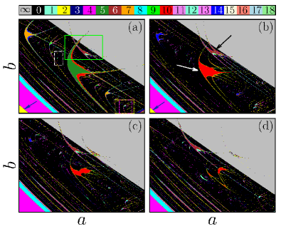
Figure 1: (Color online) Periods (see color bar) plotted in the parameter space ($a,b$) inside the interval $(a_{\mbox{\tiny min}},a_{\mbox{\tiny max}})=(1.2,1.8)$ and $(b_{\mbox{\tiny min}},b_{\mbox{\tiny max}})=(0,0.35)$, with a grid of $10^{3}\times 10^{3}$, ICs $x_{0}=0.01$ and $y_{0}=0.05$ and $N=10^{7}$ iterations, for the composition of $k=2$ MHMs using (a) $F=0$, (b) $F=7\times 10^{-3}$, (c) $F=2\times 10^{-2}$ and (d) $F=4\times 10^{-2}$.

III.1 Duplication of Shrimp-like ISSs ($k=2$)

For the duplication we use $g(F,n)=F\,(-1)^{n}$ so that the protocol is $F,-F,F,-F,\ldots$ and function $g(F,n)$ is $k=2$ periodic. Figure 1 shows the period of trajectories in the parameter space ($a,b$). Each color represents a given period (see color bar). In Fig. 1(a) the case $F=0$ is displayed and almost any ISS has shrimp-like form with distinct periods. Inside each ISS a sequence of PDBs $p\to 2p\to 4p\to\ldots,l\,p$ occurs. For a detailed description of the periods, properties of the shrimp-like ISSs shown in Fig. 1(a), we refer the readers to the work J. A. C. Gallas (1993). If parameters are chosen inside one ISS, the Hénon map will generate a stable orbit with period corresponding to the color. For example, the largest ISS in the center of Fig. 1(a) has a per-$5$, while the smaller ISS just above this per-$5$ ISS, has a per-$6$ (see green box). When parameters are chosen outside the ISSs, a chaotic motion occurs and is represented in Fig. 1 by the black color. The grey color represents the case when the trajectory diverges and no bounded motion is expected.

Results for $F=7\times 10^{-3}$ are shown in Fig. 1(b), which displays the same parameter interval from Fig. 1(a). For simplicity we have chosen to count the periods including all states. In other words, we do not display the periods of the composed map. First observation in Fig. 1(b) is that while ISSs with even periods keep their period, for all ISSs with odd periods the period is duplicated, as expected by rule (b). For example, the large shrimp-like ISS mentioned above with $p=5$ ($\omega=5/2$), has now $p_{\mbox{\tiny F}}=10$ (see white arrow). There are obviously no per-$1$ orbits anymore and orbits with odd periods-$p$ are prohibited since $\omega=p/k=p/2$ is rational. The second observation is that all ISSs with even periods $p$ start to duplicate, since $\omega=p/2$ is an integer and satisfies rule (a). This is better observed by the ISSs with periods $p=p_{\mbox{\tiny F}}=6$ ($\omega=6/2$), which separate from each other. See the black arrow indicating both ISSs. From the resolution of Fig. 1(b), some of the duplications from other ISSs cannot be seen. The separation between the duplicated ISSs in the parameter space increases with $F$, as can be checked in Fig. 1(c) for $F=2\times 10^{-2}$ and in Fig. 1(d) for $F=4\times 10^{-2}$. An interesting aspect is that the per-$6$ ISS from the right moves further to the right as $F$ increases, until it reaches the grey region where it starts to disappear. In addition, the above mentioned large shrimp-like ISS with $p_{\mbox{\tiny F}}=10$ (white arrow) is transformed into three (not a triplication in this case, see explanation bellow) interconnected shrimps observed in Fig. 1(d). Such interconnected shrimps were observed to be relevant in a tunnel diode and a fiber-ring laser Francke et al. (2013) and, in this context, endorses the importance to control the intermediate dynamics to create and enlarge the ISSs.

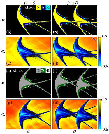
Figure 2: (Color online) Parameter space $(a,b)$ with a grid of $10^{3}\times 10^{3}$. The duplication of a per-8 ISS is presented in (a)-(d) in the interval $(a_{\mbox{\tiny min}},a_{\mbox{\tiny max}})=(1.719,1.736)$, $(b_{\mbox{\tiny min}},b_{\mbox{\tiny max}})=(0.110,0.118)$. Periods were count after a transient of $5\times 10^{6}$ iterations and are shown for (a) $F=0$ and (b) $F=2\times 10^{-3}$. The largest LE was computed using a trajectory of $5\times 10^{6}$ iterations and is displayed in (c) and (d) for same values of $F$. For a per-10 ISS in the interval $(a_{\mbox{\tiny min}},a_{\mbox{\tiny max}})=(1.6726,1.6794)$, $(b_{\mbox{\tiny min}},b_{\mbox{\tiny max}})=(0.1417,0.1441)$ the duplication is presented in (e) $F=0$ and (f) $F=8\times 10^{-4}$ using periods and in (g) and (h) using the largest LE.

III.1.1 Magnification of ISSs with integer $\omega=p/k$

To understand better the duplication of ISSs, Fig. 2 presents details of the effect of increasing values of $F$ in two distinct shrimp-like ISSs with PDBs $p=p_{\mbox{\tiny F}}=8\to 16\to 32\ldots$ ($\omega=4\to 8\to 16\ldots$) in Figs. 2(a) and (b) and $p=p_{\mbox{\tiny F}}=10\to 20\to 40\ldots$ ($\omega=5\to 10\to 20\ldots$) in Figs. 2(e) and (f). For $F\neq 0$ in both cases we obtain $k=2$ identical ISSs which are copies of the original one’s and $k=2$ attractors in phase space (see Sec. IV). To turn the statement of identical copies more convincing, we plot the largest Lyapunov exponent (LE) for each case [see Figs. 2(c),(d),(g),(h)]. Grey, yellow to red for increasing positive LE, and blue to cyan for increasing negative LE. It nicely shows that the internal structures of the ISSs, which contain information about the local stability, is unaltered by the duplication. Thus, identical copies refer to the shape of the ISSs and the corresponding stability for parameters chosen inside the ISSs.

III.1.2 Magnification of ISSs with rational $\omega=p/k$

Figure 3 presents the magnification for a shrimp-like ISS with PDB $p=7\to 14\to 26\to\ldots$ ($\omega=7/2\to 7\to 14\dots$). Here the effect of increasing values of $F$ on the ISS is more complicated since the lowest period of the PDB sequence follows rule (b), while all subsequent periods follow rule (a). Since $\omega=7/2$ for $p=7$, we obtain $p_{\mbox{\tiny F}}=2\times 7=14$, confirming rule (b). In this case only one attractor with $p_{\mbox{\tiny F}}=14$ is found and no duplication of the ISS with this period occurs. This breaks the ISS apart as observed in Figs. 3(b)-(d). While one main shrimp-like ISSs with period $p_{\mbox{\tiny F}}=14$ (and PDBs sequence $28\to 56\ldots$) remains, two smaller non-overlapping ISSs with period $p=p_{\mbox{\tiny F}}=14$ move apart (see white arrows). However, here the internal structure of the ISS is changed qualitatively when compared to the $F=0$ case, as can be checked in the largest LE analysis in Figs. 3(e)-(h).    

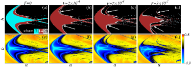
Figure 3: (Color online) Parameter space $(a,b)$ with a grid of $10^{3}\times 10^{3}$ showing the interval $(a_{\mbox{\tiny min}},a_{\mbox{\tiny max}})=(1.225,1.295)$, $(b_{\mbox{\tiny min}},b_{\mbox{\tiny max}})=(0.26,0.33)$ displaying in (a)-(d) the periods determined after a transient time of $5\times 10^{6}$ in (e)-(h) the LE computed using a trajectory of $5\times 10^{6}$ iterations.

III.2 Triplication ($k=3$), quadruplication ($k=4$) and more…

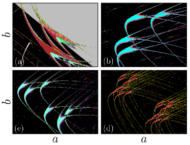
Figure 4: (Color online) Periods (see color bar in Fig. 1) plotted in the parameter space ($a,b$) with a grid of $10^{3}\times 10^{3}$ and $N=2\times 10^{6}$ iterations for (a) triplication ($k=3$) of the per-$6$ shrimp [see green box from Fig. 1(a)] inside the interval $(a_{\mbox{\tiny min}},a_{\mbox{\tiny max}})=(1.42,1.60)$ and $(b_{\mbox{\tiny min}},b_{\mbox{\tiny max}})=(0.20,0.29)$ using $F=1.2\times 10^{-3}$, (b) quadruplication ($k=4$) of the per-$8$ shrimp [see magenta box from Fig. 1(a)] for $F=2.0\times 10^{-3}$ and $(a_{\mbox{\tiny min}},a_{\mbox{\tiny max}})={(1.68,1.74)}$, $(b_{\mbox{\tiny min}},b_{\mbox{\tiny max}})={(0,0.05)}$, (c) sextuplication ($k=6$) of the per-$12$ shrimp [see white box from Fig. 1(a)] for $F=1.2\times 10^{-3}$, $(a_{\mbox{\tiny min}},a_{\mbox{\tiny max}})={(1.37,1.41)}$, $(b_{\mbox{\tiny min}},b_{\mbox{\tiny max}})={(0.18,0.23)}$ and (d) examples of the decuplications ($k=10$) of per-$10$ of two shrimp-like ISSs in the interval $(a_{\mbox{\tiny min}},a_{\mbox{\tiny max}})=(1.66,1.75)$, $(b_{\mbox{\tiny min}},b_{\mbox{\tiny max}})=(0,0.05)$ [see yellow box from Fig. 1(a)].

Next it is shown that the above behavior can be extended to multiply ISSs in the parameter space. For the triplicated case ($k=3$) the external force must have per-$3$, as can be obtained by using the protocol $-F,0,F,-F,0,F,\ldots$ perturbing the HM. In this case, the ISSs with periods multiple of $3$ are triplicated. In this section we focus on integer values of $\omega$. Results are shown in Fig. 4(a), which displays a magnification of the parameter space from Fig. 1(a) and for $F=1.2\times 10^{-3}$. This is a triplication of the per-$6$ shrimp ($\omega=6/3$). In fact, it creates $k=3$ per-$6$ stable periodic orbits which separate more and more for increasing values of $F$. In Fig. 4(b) it is shown the case of the quadruplication of the per-$8$ shrimp [see magenta box from Fig. 1(a)] using $+F,-F/2,F/2,-F,\ldots,+F,-F/2$ with $F=2.0\times 10^{-3}$. Fig.4(c) displays the sextuplication of the per-$12$ shrimp using $+F,-F/2,F/4,-F/4,F/2,-F,+F,-F/2,\ldots$ with $F=1.2\times 10^{-3}$. To show that a proliferation of the ISS is possible, we present in Fig. 4(d) the case of the decuplications of two per-10 ISSs, so that twenty ISSs are observed.

IV Multiplication of attractors and riddled basins

It remains to show that the multiplication of ISSs in the parameter space is a consequence of the multiplication of attractors in phase space. To exemplify this we show the duplication and triplication of shrimp-like ISSs from Fig. 1. Figure 5(a) shows the basin of attraction inside the per-6 ISS from Fig. 1(a) for $F=0$. Figure 5(b) shows the basin of attraction for the duplication for which the identical copies of the ISSs still overlap. We clearly observe that it generates another basin of attraction related to the duplicated per-6 orbit. Figure 5(c) shows the basin of attraction for the case of three attractors, each one with per-6.

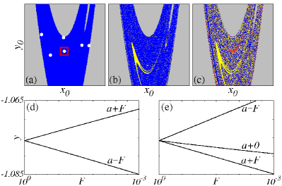
Figure 5: (Color online) The basin of attraction of the MHM plotted inside the interval $(x_{0_{\mbox{\tiny min}}},x_{0_{\mbox{\tiny max}}})=(-3.0,3.0)$ and $(y_{0_{\mbox{\tiny min}}},y_{0_{\mbox{\tiny max}}})=(-7.0,7.0)$ for $a=1.514$, $b=0.230$. In (a) we show the case $F=0$ and the white circles are the periodic points of the per-6 attractor. In (b) the duplication ($k=2$) for $F=1\times 10^{-3}$ and (c) the triplication ($k=3$) for $F=1\times 10^{-3}$. The gray color represents the ICs that lead to divergence and the regions with blue, yellow and red colors refer to different attractors due to $F\neq 0$. In (d) and (e) we show, respectively, the duplication and triplication of the orbital point from the per-6 attractor inside the red box in (a).

Figures 5(d) and (e) display, respectively, the duplication and triplication of one per-6 orbital point [see inside red box in Fig. 5(a)] as a function of $F$. It is very interesting to observe that $k$ small parametric changes in the HM generates $k$ riddled basin of attractions Alexander et al. (1992).

V Duplication of other Structures

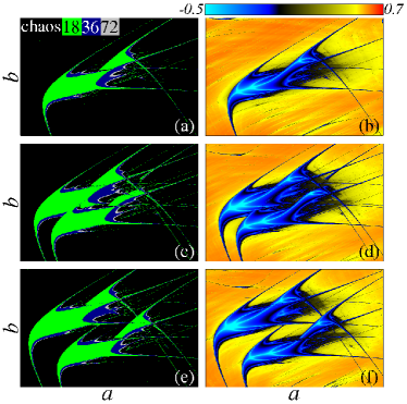
Figure 6: (Color online) Parameter space $(a,b)$ with a grid of $10^{3}\times 10^{3}$. The duplication of a per-18 ISS is presented in the interval $(a_{\mbox{\tiny min}},a_{\mbox{\tiny max}})=(1.289,1.302)$, $(b_{\mbox{\tiny min}},b_{\mbox{\tiny max}})=(0.259,0.268)$ displaying the periods in (a) $F=0$, (c) $F=6\times 10^{-4}$ and (e) $F=1\times 10^{-3}$ and the largest LE in (b), (d) and (f) for same values of $F$.

The ISSs discussed in Sec. III.1 have the well known shrimp-like form J. A. C. Gallas (1993). However, other ISSs exist which may be more complicated or not. For example, simpler ISSs than the shrimp-like are the cuspidal and non-cuspidal, shown respectively in Fig. 1(a) and Fig. 1(b) from A.Celestino et al. (2013). More complicated and higher order ISSs were described in the very last paper from Lorenz Lorenz (2008).

The purpose of the present Section is to show that our multiplication procedure is also valid for such ISSs. The first example is shown in Fig. 6 for the duplication of a per-18 ISS. Doing a visual analysis, the ISS from Fig. 6(a) for $F=0$ could be wrongly interpreted as a composition of shrimp-like ISSs which are overlapped. But this is not the case, as shown by Lorenz and checked here analyzing the LE in Fig. 6(b). Compared to the shrimp-like ISSs, now we have two superstable regimes (cyan lines) inside the ISSs. This also suggest that the dynamics inside the ISS from Fig. 6(a) is different, regarding stability, from the dynamics inside shrimp-like ISS.

As the values of $F$ increases the duplication of the ISS is visible and nice complex pictures are generated. While the inner structure of the LE inside the ISSs from Fig. 6(d) are still identical to the original one from Fig. 6(b) (compare cyan lines), this changes in Fig. 6(f). We observed in general that the higher-order ISSs are more sensitive to $F$. In other words, the duplication generates identical copies of the higher-order ISS, but they change very fast with increasing values of $F$.

Figure 7 shows the example of the duplication of a per-40 higher-order ISS. Again the duplications are visible but the copies are only identical for very small values of $F$. Both examples above are related to integer values of $\omega=p/k$, namely $18/2=9$ and $40/2=20$ respectively. Both cases obey rule (a).

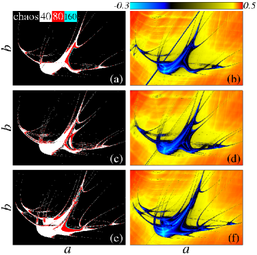
Figure 7: (Color online) Parameter space $(a,b)$ with a grid of $10^{3}\times 10^{3}$. The duplication of a per-40 ISS is presented in the interval $(a_{\mbox{\tiny min}},a_{\mbox{\tiny max}})=(1.1703,1.1722)$, $(b_{\mbox{\tiny min}},b_{\mbox{\tiny max}})=(0.3420,0.34235)$. Cases (a) $F=0$, (c) $F=2\times 10^{-6}$ and (e) $F=1\times 10^{-5}$ display the periods and (b), (d) and (f) the largest LE for same values of $F$.

VI Analytical results for $p_{\mbox{\tiny F}}=2$

For low periods it is possible to give an analytical demonstration of the duplication. Years ago the boundaries between the born of per-$1$ and the PDBs $1\to 2$ and $2\to 4$ were determined analytically in the parameter space of the Hénon map. These boundaries are given by the relations Beims and Gallas (1997); Gallas (1995):

$$W_{1}(a,b) = (4a+1-2b+b^{2})=0,$$ (2)

$$W_{1\to 2}(a,b) = (4a-3+6b-3b^{2})^{3}=0,$$

$$W_{2\to 4} (a,b)=(4a-5+6b-5b^{2})^{2}\times[5b^{4}+4b^{3}+$$ (4)

$$(8a-2)b^{2}+(16a+4)b+16a^{2}+8a+5]\,=0.$$

Compared to the original work, last equation includes a polynomial with complex solutions for ($a,b$). This polynomial must be taken into account in case $F\neq 0$. Applying the same procedure for the duplication in MHM we obtain

$$W_{p_{\mbox{\tiny F}}=2}(a,b,F)=W_{1}(a,b)W_{1\to 2}(a,b)+256F^{4}-$$ (5)

$$\qquad[288b^{4}-1152b^{3}+(1536a+1728)b^{2}-(3072a+$$ (6)

$$\qquad 1152)b+512a^{2}+1536a+288]F^{2}=0,$$ (7)

(8)

$$W_{p_{\mbox{\tiny F}}=2\to 4}(a,b,F)=W_{2\to 4}(a,b)+256F^{4}-[160b^{4}-$$ (9)

$$\qquad 1152b^{3}+(1536a+1472)b^{2}-(3072a+1152)b+$$ (10)

$$\qquad 512a^{2}+1536a+160]F^{2}=0.$$ (11)

Equation (5) gives the birth (saddle-node bifurcation) of per-1 orbits for the map composed of two iterations of the MHM ($p_{\mbox{\tiny F}}=2$) and Eq. (8) indicates the PDB from period 1 to 2 for the composed map, which for the iterations of MHMs means $p_{\mbox{\tiny F}}=2\to 4$. The solution of Eq. (8) is indicated with blue arrows in Fig. 1(a) for $F=0$ and in Fig. 1(b) for $F=7\times 10^{-3}$. Interesting to observe that for $F\neq 0$ the boundaries $W_{1}(a,b)$ and $W_{1\to 2}(a,b)$ become coupled in Eq. (5). In other words, the two independent conditions $W_{1}(a,b)=0$ for saddle-node bifurcation and $W_{1\to 2}(a,b)=0$ for PDB, are transformed in one saddle-node bifurcation condition $W_{p_{\mbox{\tiny F}}=2}(a,b,F)=0$. Therefore the PDB $1\to 2$ from $F=0$ becomes forbidden.

To explain this better we show an example using $b=0.3$ and $F=0.01$. The solutions for the first boundaries and $F=0$ are

$$W_{1}(a,0.3):a=-0.1225,\quad W_{1\to 2}(a,0.3):a=0.3675,$$

while the solutions for $F=0.01$ become

$$W_{p_{\mbox{\tiny F}}=2}(a,0.3,0.01):a=-0.1224\quad\mbox{and}\quad a=0.4377.$$

This shows that the birth of ${p_{\mbox{\tiny F}}=2}$ is shifted to the left ($-0.1225\to-0.1224$) and the PDB $1\to 2$ at $a=0.3675$ becomes forbidden (since $\omega=1/2$), transforming it into a saddle-node bifurcation at $a=0.4377$. Thus, for $F=0.01$ we have two saddle-node bifurcating points. The other boundaries are given by

$$W_{2\to 4}(a,0.3):a=0.9125\,\,\mbox{and}\,\,a=-0.4225\pm i\,0.4550,$$ (12)

(13)

$$W_{p_{\mbox{\tiny F}}=2\to 4}(a,0.3,0.01):a=0.8983\,\,\mbox{and}\,\,a=0.9267,$$

which shows that the complex solution from the $F=0$ case becomes real and we end up wit two PDBs $2\to 4$, one in $a=0.8983$ and the other one in $a=0.9267$. This explains the origin of the duplication of the PDBs sequence and of the ISSs which contain them. For more simples examples of the origin of shifted bifurcation diagrams via prohibition of PDBs we refer the reader to the one-dimensional case da Silva et al. (2017).

VII Conclusions

In this work we show that the parametric control in composed maps can be used to enlarge stable domains in phase and parameter spaces of two-dimensional discrete nonlinear dynamical systems. Since the stable domains in parameter space are generic, our results are expected to be applicable to a large number of systems. We present analytical and numerical results for the specific case of the composition of Hénon maps with distinct parameters. Using the composition of $k$ Hénon maps with distinct parameters we have observed following properties: (1) When the ratio $\omega=p/k$ is an integer, where $p$ is the period of the stable orbit, $k$-identical attractors in phase space and $k$-identical ISSs in parameters space are generated. The identical copies are split apart as a function of the parameter $F$. The equivalence between identical stable attractors and identical ISSs was checked by the largest LE analysis. Besides that, the additional basin of attraction regarding to the identical copies of the ISSs are riddled. (2) When the ratio $\omega$ is not an integer, the number of attractors in phase space and ISSs in parameter space remain unaltered. The new orbital period is $p_{\mbox{\tiny F}}=k\,p$ and the multiplied ISS is broken apart. (3) The sign of the parameters from the intermediate dynamics must change by each iteration, otherwise no multiplication is observed.

The multiple composition of maps lead to the appearance of multiple attractors in phase space and multiple shifted ISSs in the parameter space. Consequently occurs a considerable enlargement of the stable domains in phase and parameter spaces. This is crucial for the survival of the desired dynamics under noise and temperature effects, which usually destroy the ISSs starting from their borders Manchein et al. (2013) (also observed in the parameter space of the relativistic standard map Horstmann et al. (2017)). Future contributions intend to verify the enlargement of stable domains for practical applications submitted to thermal effects. The multiple composition of Hénon maps may be related to the general Jung’s decomposition Friedland and Milnor (1989), which shows that any planar, invertible quadratic map can be reduced to a composition of Henon-like maps. However, it is not the purpose of the present work to show such relation.