Linear algebraic analogues of
the graph isomorphism problem and the Erdős-Rényi model

Abstract

A classical difficult isomorphism testing problem is to test isomorphism of $p$-groups of class $2$ and exponent $p$ in time polynomial in the group order. It is known that this problem can be reduced to solving the alternating matrix space isometry problem over a finite field in time polynomial in the underlying vector space size. We propose a venue of attack for the latter problem by viewing it as a linear algebraic analogue of the graph isomorphism problem. This viewpoint leads us to explore the possibility of transferring techniques for graph isomorphism to this long-believed bottleneck case of group isomorphism.

In 1970’s, Babai, Erdős, and Selkow presented the first average-case efficient graph isomorphism testing algorithm (SIAM J Computing, 1980). Inspired by that algorithm, we devise an average-case efficient algorithm for the alternating matrix space isometry problem over a key range of parameters, in a random model of alternating matrix spaces in vein of the Erdős-Rényi model of random graphs. For this, we develop a linear algebraic analogue of the classical individualisation technique, a technique belonging to a set of combinatorial techniques that has been critical for the progress on the worst-case time complexity for graph isomorphism, but was missing in the group isomorphism context. As a consequence of the main algorithm, we establish a weaker linear algebraic analogue of Erdős and Rényi’s classical result that most graphs have the trivial automorphism group. We also show that Luks’ dynamic programming technique for graph isomorphism (STOC 1999) can be adapted to slightly improve the worst-case time complexity of the alternating matrix space isometry problem in a certain range of parameters.

Most notable progress on the worst-case time complexity of graph isomorphism, including Babai’s recent breakthrough (STOC 2016) and Babai and Luks’ previous record (STOC 1983), has relied on both group theoretic and combinatorial techniques. By developing a linear algebraic analogue of the individualisation technique and demonstrating its usefulness in the average-case setting, the main result opens up the possibility of adapting that strategy for graph isomorphism to this hard instance of group isomorphism. The linear algebraic Erdős-Rényi model is of independent interest and may deserve further study. In particular, we indicate a connection with enumerating $p$-groups of class $2$ and exponent $p$.

1 Introduction

1.1 Problems, postulates, and models

Let $\mathbb{F}_{q}$ be the finite field with $q$ elements. An $n\times n$ matrix $A$ over $\mathbb{F}_{q}$ is alternating, if for every $u\in\mathbb{F}_{q}^{n}$, ${u}^{\mathrm{t}}Au=0$. $\Lambda(n,q)$ denotes the linear space of $n\times n$ alternating matrices over $\mathbb{F}_{q}$, and a dimension-$m$ subspace of $\Lambda(n,q)$ is called an $m$-alternating (matrix) space. $\mathrm{GL}(n,q)$ denotes the general linear group of degree $n$ over $\mathbb{F}_{q}$. We study the following problem.

Problem 1 (Alternating matrix space isometry problem, AltMatSpIso).

Given the linear bases of two $m$-alternating spaces $\mathcal{G},\mathcal{H}$ in $\Lambda(n,q)$, decide whether there exists $A\in\mathrm{GL}(n,q)$, such that ${A}^{\mathrm{t}}\mathcal{G}A:=\{{A}^{\mathrm{t}}BA:B\in\mathcal{G}\}$ is equal to $\mathcal{H}$ as subspaces.

If such an $A$ exists, we say that $\mathcal{G}$ and $\mathcal{H}$ are isometric. As will be explained in Section 1.2, AltMatSpIso has been studied, mostly under other names, for decades. It lies at the heart of the group isomorphism problem (GroupIso), and has an intimate relationship with the celebrated graph isomorphism problem (GraphIso). As a problem in ${\rm NP}\cap{\rm coAM}$, its worst-case time complexity has barely been improved over the brute-force algorithm. In fact, a $q^{O(n+m)}$-time algorithm is already regarded as very difficult.

Let us recall one formulation of GraphIso. For $n\in\mathbb{N}$, let $[n]=\{1,2,\dots,n\}$, and $S_{n}$ denotes the symmetric group on $[n]$. A simple undirected graph is just a subset of $\Lambda_{n}:=\{\{i,j\}:i,j\in[n],i\neq j\}$. A permutation $\sigma\in S_{n}$ induces a natural action on $\Lambda_{n}$. The following formulation of GraphIso as an instance of the setwise transporter problem is well-known [Luk82].

Problem 2 (Graph isomorphism problem, GraphIso).

Given two subsets $G,H$ of $\Lambda_{n}$, decide whether there exists $\sigma\in S_{n}$, such that $G^{\sigma}:=\{\{i^{\sigma},j^{\sigma}\}:\{i,j\}\in G\}$ is equal to $H$ as sets.

The formulations of AltMatSpIso and GraphIso as in Problem 1 and Problem 2 lead us to the following postulate.

Postulate 1.

AltMatSpIso can be viewed and studied as a linear algebraic analogue of GraphIso.

Postulate 1 originates from the following meta-postulate.

Meta-postulate.

Alternating matrix spaces can be viewed and studied as a linear algebraic analogue of graphs.

This meta-postulate will be studied further in [Qia17]. As a related note, recent progress on the non-commutative rank problem suggests the usefulness of viewing linear spaces of matrices as a linear algebraic analogue of bipartite graphs [GGOW16, IQS16, IQS17].

From the meta-postulate, we formulate a model of random alternating matrix spaces over $\mathbb{F}_{q}$. Let ${\genfrac{[}{]}{0.0pt}{}{\ }{\ }}_{q}$ be the Gaussian binomial coefficient with base $q$.

Model 1 (The linear algebraic Erdős-Rényi model).

The linear algebraic Erdős-Rényi model, $\mbox{\sc LinER}(n,m,q)$, is the uniform probability distribution over the set of dimension-$m$ subspaces of $\Lambda(n,q)$, that is, each subspace is endowed with probability $1/{\genfrac{[}{]}{0.0pt}{}{\binom{n}{2}}{m}}_{q}$.

Model 1 clearly mimics the usual Erdős-Rényi model [ER59, ER63, Bol01].

Model 2 (Erdős-Rényi model).

The Erdős-Rényi model $\mbox{\sc ER}(n,m)$ is the uniform probability distribution over the set of size-$m$ subsets of $\Lambda_{n}$, that is, each subset is endowed with probability $1/\binom{\binom{n}{2}}{m}$.

We then pose the following postulate.

Postulate 2.

$\mbox{\sc LinER}(n,m,q)$ can be viewed and studied as a linear algebraic analogue of $\mbox{\sc ER}(n,m)$.

1.2 Background of the alternating matrix space isometry problem

While the name AltMatSpIso may be unfamiliar to some readers, this problem has been studied for decades as an instance – in fact, the long-believed bottleneck case – of the group isomorphism problem. This problem also has an intricate relationship with the graph isomorphism problem. We first review these connections below, and then examine the current status of this problem.

Relation with the group isomorphism problem.

We first introduce the group isomorphism problem (GroupIso) and mention a long-believed bottleneck instance of this problem. It turns out that AltMatSpIso is almost equivalent to this instance.

GroupIso asks to decide whether two finite groups of order $n$ are isomorphic or not. The difficulty of this problem depends crucially on how we represent the groups in the algorithms. If our goal is to obtain an algorithm running in time $\mathrm{poly}(n)$, then we may assume that we have at our disposal the Cayley (multiplication) table of the group, as we can recover the Cayley table from most reasonable models for computing with finite groups. Therefore, in the main text we restrict our discussion to this very redundant model, which is meaningful mainly because we do not know a $\mathrm{poly}(n)$-time or even an $n^{o(\log n)}$-time algorithm [Wil14] ($\log$ to the base $2$), despite that a simple $n^{\log n+O(1)}$-time algorithm has been known for decades [FN70, Mil78]. The past few years have witnessed a resurgence of activity on algorithms for this problem with worst-case analyses in terms of the group order; we refer the reader to [GQ17a] which contains a survey of these algorithms.

It is long believed that $p$-groups form the bottleneck case for GroupIso. In fact, the decades-old quest for a polynomial-time algorithm has focused on class-$2$ $p$-groups, with little success. Even if we restrict further to consider $p$-groups of class $2$ and exponent $p$, the problem is still difficult. Recent works [LW12, BW12, BMW15, IQ17] solve some nontrivial subclasses of this group class, and have lead to substantial improvement in practical algorithms. But the methods in those works seem not helpful enough to lead to any improvement for the worst-case time complexity of the general class.

By a classical result of Baer [Bae38], testing isomorphism of $p$-groups of class $2$ and exponent $p$ in time polynomial in the group order reduces to solving AltMatSpIso over $\mathbb{F}_{p}$ in time $p^{O(m+n)}$. On the other hand, there also is an inverse reduction for $p>2$. In fact, when such $p$-groups are given by generators in the permutation group quotient model [KL90], isomorphism testing reduces to solving AltMatSpIso in time $\mathrm{poly}(n,m,\log p)$ [BMW15]. We will recall the reductions in Appendix A. Because of these reductions and the current status of GroupIso, we see that AltMatSpIso lies at the heart of GroupIso, and solving AltMatSpIso in $q^{O(m+n)}$ is already very difficult.

Relation with the graph isomorphism problem.

The celebrated graph isomorphism problem (GraphIso) asks to decide whether two undirected simple graphs are isomorphic. The relation between AltMatSpIso and GraphIso is very delicate. Roughly speaking, the two time-complexity measures of AltMatSpIso, $q^{O(n+m)}$ and $\mathrm{poly}(n,m,q)$, sandwiches GraphIso in an interesting way. For one direction, solving AltMatSpIso in time $q^{O(n+m)}$ can be reduced to solving GraphIso for graphs of size $q^{O(n+m)}$, by first reducing to solving GroupIso for groups of order $q^{O(n+m)}$ as above, and then to solving GraphIso for graphs of size $q^{O(n+m)}$ by the reduction from GroupIso to GraphIso [KST93]. Therefore, a polynomial-time algorithm for GraphIso implies an algorithm for AltMatSpIso in time $q^{O(n+m)}$. It is then reasonable to examine whether the recent breakthrough of Babai [Bab16, Bab17], a quasipolynomial-time algorithm for GraphIso, helps with reducing the time complexity of AltMatSpIso. This seems unlikely. One indication is that the brute-force algorithm for AltMatSpIso is already quasipolynomial with respect to $q^{O(n+m)}$. Another evidence is that Babai in [Bab16, arXiv version 2, Section 13.2] noted that his algorithm seemed not helpful to improve GroupIso, and posed GroupIso as one roadblock for putting GraphIso in P. Since AltMatSpIso captures the long-believed bottleneck case for GroupIso, the current results for GraphIso are unlikely to improve the time complexity to $q^{O(n+m)}$. There is also an explanation from the technical viewpoint [GR16]. Roughly speaking, the barrier in the group theoretic framework for GraphIso is to deal with large alternating groups, as other composition factors like projective special linear groups can be handled by brute-force in quasipolynomial time, so for the purpose of a quasipolynomial-time algorithm these group are not a concern. On the other hand for AltMatSpIso it is exactly the projective special linear groups that form a bottleneck. For the other direction, in a forthcoming work [GQ17b], it is shown that solving GraphIso in polynomial time reduces to solving AltMatSpIso over $\mathbb{F}_{q}$ with $q=\mathrm{poly}(n)$ in time $\mathrm{poly}(n,m,q)$.

Current status of AltMatSpIso.

It is not hard to show that solving AltMatSpIso in time $\mathrm{poly}(n,m,\log q)$ is in ${\rm NP}\cap{\rm coAM}$, so it is unlikely to be ${\rm NP}$-complete. As to the worst-case time complexity, the brute-force algorithm for AltMatSpIso runs in time $q^{n^{2}}\cdot\mathrm{poly}(m,n,\log q)$. Another analysed algorithm for AltMatSpIso offers a running time of $q^{\frac{1}{4}(n+m)^{2}+O(n+m)}$ when $q=p$ is a prime, by first reducing to testing isomorphism of class-$2$ and exponent-$p$ $p$-groups of order $p^{n+m}$, and then applying Rosenbaum’s $N^{\frac{1}{4}\log_{p}N+O(1)}$-time algorithm for $p$-groups of order $N$ [Ros13]. This is only better than the brute-force one when $m<n$. It is somewhat embarrassing that for a problem in ${\rm NP}\cap{\rm coAM}$, we are only able to barely improve over the brute-force algorithm in a limited range of parameters. In a very true sense, our current understanding of the worst-case time complexity of AltMatSpIso is like the situation for GraphIso in the 1970’s.

On the other hand practical algorithms for AltMatSpIso have been implemented. As far as we know, current implemented algorithms for AltMatSpIso can handle the case when $m+n\approx 20$ and $p\approx 13$, but absolutely not the case if $m+n\approx 200$, though for $m+n\approx 200$ and say $p\approx 13$ the input can be stored in a few megabytes. For GraphIso, the programs Nauty and Traces [MP14] can test isomorphism of graphs stored in gigabytes in a reasonable amount of time. Therefore, unlike GraphIso, AltMatSpIso seems hard even in the practical sense.

On the parameters.

From the discussion above, we see that solving AltMatSpIso with a worst-case time complexity $q^{O(n+m)}$ seems already a difficult target. From the meta-postulate, it is helpful to think of vectors in $\mathbb{F}_{q}^{n}$ as vertices, and matrices in an $m$-alternating space as edges, so the $q^{O(n+m)}$ measure can be thought of as polynomial in the number of “vertices” and the number of “edges.” Here the parameter $m$ comes into the theme, because $q^{m}$, while no more than $q^{\binom{n}{2}}$, is not necessarily bounded by a polynomial in $q^{n}$. This is in contrast to GraphIso, where the edge number is at most quadratic in the vertex number. In particular, when $m=\Omega(n^{2})$, the brute-force algorithm which runs in $q^{n^{2}}\cdot\mathrm{poly}(m,n,\log q)$ is already in time $q^{O(n+m)}$. Furthermore, if we consider all $n\times n$ alternating matrix spaces (regardless of the dimension), most of them are of dimension $\Omega(n^{2})$, so the brute-force algorithm already works in time $q^{O(n+m)}$ for most alternating matrix spaces. On the other hand, when $m$ is very small compared to $n$, say $m=O(1)$, we can enumerate all elements in $\mathrm{GL}(m,q)$ in time $q^{O(1)}$, and apply the isometry testing for alternating matrix tuples from [IQ17] which runs in randomized time $\mathrm{poly}(n,m,\log q)$. Therefore, the $q^{O(n+m)}$-time measure makes most sense when $m$ is comparable with $n$, in particular when $m=\Theta(n)$. This is why we study average-case algorithms in this regime of parameters (e.g. $\mbox{\sc LinER}(n,m,q)$ with $m=\Theta(n)$), while the average-case algorithm for GraphIso in [BES80] considers all graphs (e.g. each labelled graph is taken with probability $1/2^{\binom{n}{2}}$).

1.3 Algorithmic results

Postulates 1 and 2 seem hopeful at first sight by the formulations of AltMatSpIso and LinER. But realities in the combinatorial world and the linear algebraic world can be quite different, as just discussed in the last paragraph. So meaningful results cannot be obtained by adapting the results for graphs to alternating matrix spaces in a straightforward fashion. One purpose of this article is to provide evidence that, despite potential technical difficulties, certain ideas that have been developed for GraphIso and ER can be adapted to work with AltMatSpIso and LinER.

We will take a shortcut, by presenting one result that supports both postulates. In the graph setting, such a result is naturally an average-case efficient graph isomorphism testing algorithm with the average-case analysis done in the Erdős-Rényi model. The first such algorithm was proposed by Babai, Erdős and Selkow in 1970’s [BES80], with follow-up improvements by Lipton [Lip78], Karp [Kar79], and Babai and Kučera [BK79]. Therefore we set to study average-case algorithms for AltMatSpIso in the LinER model. Inspired by the algorithm in [BES80], we show the following.

Theorem 1 (Main result).

Suppose $m=cn$ for some constant $c$. There is an algorithm which, for almost but at most $1/q^{\Omega(n)}$ fraction of alternating matrix spaces $\mathcal{G}$ in $\mbox{\sc LinER}(n,m,q)$, tests any alternating matrix space $\mathcal{H}$ for isometry to $\mathcal{G}$ in time $q^{O(n)}$.

An important ingredient in Theorem 1, the utility of which should go beyond the average-case setting, is an adaptation of the individualisation technique for GraphIso to AltMatSpIso. We also realise a reformulation of the refinement technique for GraphIso as used in [BES80] in the AltMatSpIso setting. Individualisation and refinement are very influential combinatorial ideas for GraphIso, have been crucial in the progress of the worst-case time complexity of GraphIso, including Babai’s recent breakthrough [Bab16, Bab17], but were missing in the GroupIso context.

The main contribution of this article to AltMatSpIso is to initiate the use of the individualisation and refinement ideas for GraphIso in this problem.

Here, we note an interesting historical coincidence. Babai was the first to import the group theoretic idea to GraphIso in 1979 [Bab79], by when the combinatorial techniques had been around for quite some time. On the other hand, we have an opposite situation for AltMatSpIso: the relevant group theoretic tools have been the subject of intensive study for decades, while it is the combinatorial individualisation and refinement ideas that need to be imported. We do understand though, that there are valid reasons for people not having come to this before. For example, we would not have come to such ideas, if we restrict ourselves to solving AltMatSpIso in time $\mathrm{poly}(n,m,\log q)$. In Section 8.1, we will reflect on the historical development on the worst-case complexity of GraphIso, and discuss the prospect of getting a $q^{O(n^{2-\epsilon})}$-time algorithm for AltMatSpIso.

For an $m$-alternating space $\mathcal{G}$ in $\Lambda(n,q)$, define the autometry group of $\mathcal{G}$, $\mathrm{Aut}(\mathcal{G})$ as $\{A\in\mathrm{GL}(n,q):A^{t}\mathcal{G}A=\mathcal{G}\}$. The proof of Theorem 1 implies the following, which can be viewed as a weaker correspondence of the classical result that most graphs have trivial automorphism groups [ER63].

Corollary 2.

Suppose $m=cn$ for some constant $c$. All but $1/q^{\Omega(n)}$ fraction of alternating matrix spaces in $\mbox{\sc LinER}(n,m,q)$ have autometry groups of size $q^{O(n)}$.

We observe that Corollary 2 has certain consequences to the enumeration of finite $p$-groups of class $2$. For details see Section 8.3.

Finally, we provide another piece of evidence to support Postulate 1, by adapting Luks’ dynamic programming technique for GraphIso [Luk99] to AltMatSpIso. In the GraphIso setting, this technique improves the naive $n!\cdot\mathrm{poly}(n)$ time bound to the $2^{O(n)}$ time bound, which can be understood as replacing the number of permutations $n!$ with the number of subsets $2^{n}$. In the linear algebraic setting the analogue would be to replace $\Theta(q^{n^{2}})$, the number of invertible matrices over $\mathbb{F}_{q}$, with the number of subspaces in $\mathbb{F}_{q}^{n}$ which is $q^{\frac{1}{4}n^{2}+O(n)}$. We show that this is indeed possible.

Theorem 3.

There exists a deterministic algorithm for AltMatSpIso in time $q^{\frac{1}{4}(m^{2}+n^{2})+O(m+n)}$.

Note that the quadratic term on the exponent of the algorithm in Theorem 3 is $\frac{1}{4}(m^{2}+n^{2})$, slightly better than the one based on Rosenbaum’s result [Ros13] which is $\frac{1}{4}(m+n)^{2}$. We stress though that our intention to present this result is to support Postulate 1.

Organisation of this paper.

In Section 2, we explain the basic idea the algorithm for Theorem 1, by drawing analogues with the algorithm in [BES80]. Then, after presenting preliminaries and preparation material, we present detailed proofs for Theorem 1 (Section 6) and Theorem 3 (Section 7). Section 8 includes discussions, future directions, and connections to group enumeration.

2 Outline of the main algorithm

We now describe the outline of the algorithm for Theorem 1, which is inspired by the first average-case efficient algorithm for GraphIso by Babai, Erdős, and Selkow [BES80]. We will recall the idea in [BES80] that is relevant to us, define a linear algebraic individualisation, and propose a reformulation of the refinement step in [BES80]. Then we present an outline of the main algorithm. During the procedure we will also see how the meta-postulate guides the generalisation here.

2.1 A variant of the naive refinement algorithm as used in [BES80]

Two properties of random graphs are used in the average-case analysis of the algorithm in [BES80]. The first property is that most graphs have the first $\lceil 3\log n\rceil$ largest degrees distinct. The second property, which is relevant to us, is the following.

Let $G=([n],E)$ be a simple and undirected graph. Let $r=\lceil 3\log n\rceil$, and $S=[r]$, $T=[n]\setminus[r]$. Let $B$ be the bipartite graph induced by the cut $[r]\cup\{r+1,\dots,n\}$, that is, $B=(S\cup T,F)$ where $F=\{(i,j):i\in S,j\in T,\{i,j\}\in E\}$. For each $j\in T$, assign a length-$r$ bit string $f_{j}$ as follows: $f_{j}\in\{0,1\}^{r}$ such that $f_{j}(i)=1$ if and only if $(i,j)\in F$. It is easy to verify that, all but at most $O(1/n)$ fraction of graphs satisfy that $f_{j}$’s are distinct over $j\in T$.

Let us see how the second property alone, together with the individualisation and refinement heuristic, give an average-case algorithm in $n^{O(\log n)}$. Suppose $G$ satisfies the second property, and we would like to test isomorphism between $G=([n],E)$ and an arbitrary graph $H=([n],E^{\prime})$. Let $St_{G}\subseteq\{0,1\}^{r}$ be the set of bit strings obtained in the procedure above. Note that $|St_{G}|=n-r$. In the individualising step, we enumerate all $r$-tuple of vertices in $H$. For a fixed $r$-tuple $(i_{1},\dots,i_{r})\in[n]^{r}$, we perform the refinement step, that is, label the remaining vertices in $H$ according to their adjacency relations with the $r$-tuple $(i_{1},\dots,i_{r})$ as before, to obtain another set of bit-strings $St_{H}$. If $St_{G}\neq St_{H}$ we neglect this $r$-tuple. If $St_{G}=St_{H}$, then form a bijective map between $[n]$ and $[n]$, by mapping $j$ to $i_{j}$ for $j\in[r]$, and the rest according to their labels. Finally check whether this bijective map induces an isomorphism.

It can be verified easily that the above algorithm is an $n^{O(\log n)}$-time algorithm that tests isomorphism between $G$ and $H$ given that $G$ satisfies the required property. In particular, this implies that for such $G$, $|\mathrm{Aut}(G)|\leq n^{O(\log n)}$. To recover the algorithm in [BES80], assuming that the largest $r$ degrees are distinct, one can canonicalise the choice of the $r$-tuples by choosing the one with largest $r$ degrees for both $G$ and $H$.

2.2 Individualisation and refinement in the AltMatSpIso setting

We will generalise the above idea to the setting of AltMatSpIso. To do this, we first make sense of what individualisation means in the alternating space setting. We discuss how the refinement step may be generalised, and indicate how we follow an alternative formulation of it.

Let $G=([n],E)$ and $H=([n],E^{\prime})$ be two graphs for which we want to test isomorphism. Let $\mathcal{G},\mathcal{H}\leq\Lambda(n,q)$ be two $m$-alternating spaces for which we want to test isometry. As the case in Section 2.1, we will look for properties of $G$ or $\mathcal{G}$ which enable the average-case analysis, and perform individualisation on $H$ or $\mathcal{H}$ side.

For $i\in[n]$, $e_{i}$ denotes the $i$th standard basis vector of $\mathbb{F}_{q}^{n}$. For a vector space $V$ and $S\subseteq V$, we use $\langle S\rangle$ to denote the linear span of $S$ in $V$.

Individualisation. In the graph setting, individualising $r$ vertices in $H$ can be understood as follows. First we fix a size-$r$ subset $L$ of $[n]$. Then put an order on the elements in $L$. The result is a tuple of distinct vertices $(i_{1},\dots,i_{r})\in[n]^{r}$. Enumerating such tuples incurs a multiplicative cost of at most $n^{r}$.

In the alternating matrix space setting, it is helpful to think of vectors in $\mathbb{F}_{q}^{n}$ as vertices, and matrices in $\mathcal{H}$ as edges. Consider the following procedure. First fix a dimension-$r$ subspace $L$ of $\mathbb{F}_{q}^{n}$. Then choose an ordered basis of $L$. The result is a tuple of linearly independent vectors $(v_{1},\dots,v_{r})$, $v_{i}\in\mathbb{F}_{q}^{n}$, such that $L=\langle v_{1},\dots,v_{r}\rangle$. This incurs a multiplicative cost of at most $q^{rn}$. Up to this point, this is in complete analogy with the graph setting. We may stop here and say that an $r$-individualisation amounts to fix an $r$-tuple of linearly independent vectors.

We can go a bit further though. As will be clear in the following, it is beneficial if we also fix a complement subspace $R$ of $L$, e.g. $R\leq\mathbb{F}_{q}^{n}$ such that $L\cap R=\mathbf{0}$ and $\langle L\cup R\rangle=\mathbb{F}_{q}^{n}$. This adds another multiplicative cost of $q^{r(n-r)}$, which is the number of complement subspaces of a fixed dimension-$r$ subspace in $\mathbb{F}_{q}^{n}$. In the graph setting, this step is not necessary, because for any $L\subseteq[n]$ there exists a unique complement subset $R=[n]\setminus L$.

To summarise, by an $r$-individualisation, we mean choosing a direct sum decomposition $\mathbb{F}_{q}^{n}=L\oplus R$ where $\dim(L)=r$ and $\dim(R)=n-r$, together with an ordered basis $(v_{1},\dots,v_{r})$ of $L$. Enumerating all $r$-individualisations incurs a total multiplicative cost of at most $q^{2rn-r^{2}}$.

Towards a refinement step as in [BES80].

In the GraphIso setting, individualising $r$ vertices gives $(i_{1},\dots,i_{r})\in[n]^{r}$, and allows us to focus on isomorphisms that respect this individualisation, namely those $\phi\in\mathrm{Iso}(G,H)$ such that $\phi(j)=i_{j}$ for $j\in[r]$. There are at most $(n-r)!$ such isomorphisms. Since $r$ is usually set as a polylog, just naively trying all such permutations does not help. Therefore the individualisation is usually accompanied with a refinement type technique. Specifically, setting $L=\{i_{1},\dots,i_{r}\}$ and $R=[n]\setminus L$, the refinement step as in [BES80] assigns every $v\in R$ a label according to its adjacency relation w.r.t. $(i_{1},\dots,i_{r})$. This label in fact represents a subset of $L$, and an individualisation-respecting isomorphism has to preserve this adjacency relation for every $v\in R$. This restriction turns out to be quite severe for most graphs: as observed in Section 2.1, for most graphs $G$, the adjacency relations between $(1,2,\dots,r)$ and $j\in[n]\setminus[r]$ are completely different over $j$. For such $G$ and any individualisation of $H$, this means that there is at most one way to extend $\phi(j)=i_{j}$ for $j\in[r]$ to an isomorphism between $G$ and $H$.

In the AltMatSpIso setting, an $r$-individualisation also allows us to focus on isometries that respect the decomposition $L\oplus R$ and the ordered basis $(v_{1},\dots,v_{r})$ of $L$, namely those $\phi\in\mathrm{Iso}(\mathcal{G},\mathcal{H})$ such that $\phi(e_{i})=v_{i}$ for $i\in[r]$, and $\phi(\langle e_{r+1},\dots,e_{n}\rangle)=R$. There are at most $q^{(n-r)^{2}}$ such isometries. Since $r$ will be also set to be very small – in fact a constant here – we also need some refinement type argument. For $u\in R$, we can record its “adjacency relation” w.r.t. $\mathbf{v}=(v_{1},\dots,v_{r})$ as a subspace of $L\cong\mathbb{F}_{q}^{r}$ as follows. For $Q\in\mathcal{H}\leq\Lambda(n,q)$, define $Q(\mathbf{v},u):=({v}^{\mathrm{t}}_{1}Qu,\dots,{v}^{\mathrm{t}}_{r}Qu)^{\mathrm{t}}\in\mathbb{F}_{q}^{r}$, and $\mathcal{H}(\mathbf{v},u):=\{Q(\mathbf{v},u):Q\in\mathcal{H}\}$ which is a subspace in $\mathbb{F}_{q}^{r}$. $\mathcal{H}(\mathbf{v},u)$ records the adjacency relation between $(v_{1},\dots,v_{r})$ and $u$ under $\mathcal{H}$. It can be verified that an individualisation-respecting isometry has to preserve this adjacency relation. It is tempting to check then on the $\mathcal{G}$ side, where we have the standard individualisation $(e_{1},\dots,e_{r})$ and $\langle e_{r+1},\dots,e_{n}\rangle$, whether for most $\mathcal{G}$’s it is the case that every $v\in\langle e_{r+1},\dots,e_{n}\rangle$ gets a unique label. If this is so, then the number of individualisation-respecting isomorphisms can also be significantly reduced. However, this cannot be the case when $r$ is small, as there are $q^{(n-r)^{2}}$ vectors in $R$ but there at at most $q^{r^{2}}$ subspaces in $\mathbb{F}_{q}^{r}$.

The alert reader will note that, since we are looking for linear maps from $\langle e_{r+1},\dots,e_{n}\rangle$ to $R$, the above counting argument does not make much sense, as it mostly concerns setwise maps from $\langle e_{r+1},\dots,e_{n}\rangle$ to $R$. It is indeed the case, and we further note that the map from $u\in R$ to $\mathcal{H}(\mathbf{v},u)\leq\mathbb{F}_{q}^{r}$ defines a sheaf over the projective space $\mathbb{P}(R)$, so such labels have some nontrivial relation to glue together to form a sheaf. (See the related concept of kernel sheaves as in [KV12].) It may be possible to use these observations to define a reasonable refinement step in the alternating matrix space setting. In this paper we shall follow the following reformulation.

A reformulation of the refinement step.

To resolve the above problem, we reformulate the idea in the graph setting as follows. Recall that on the $G$ side we start with the standard individualisation $[r]\cup\{r+1,\dots,n\}$ with an order on $[r]$ as $(1,\dots,r)$, and let $S=[r]$, $T=\{r+1,\dots,n\}$. This defines the bipartite graph $B=(S\cup T,F)$ where the edge set $F$ is induced from $G$. For a fixed individualisation on the $H$ side, which produces $L\cup R$, $L=\{i_{1},\dots,i_{r}\}\subseteq[n]$ with an order on $L$, this also defines a bipartite graph $C=(L\cup R,F^{\prime})$ where $F^{\prime}$ is induced from $H$. A bijective $\psi:T\to R$ is a right-side isomorphism between $B$ and $C$ if it induces an isomorphism between $B$ and $C$ as bipartite graphs. Let $\mathrm{RIso}(B,C)$ be the set of right-side isomorphisms, and let $\mathrm{IndIso}(G,H)$ be the set of individualisation-respecting isomorphisms from $G$ to $H$ w.r.t the above individualisations. Note that both $\mathrm{RIso}(B,C)$ and $\mathrm{IndIso}(G,H)$ can be embedded to the set of bijective maps between $T$ and $R$. The key observation is that an individualisation-respecting isomorphism has to be a right-side isomorphism between $B$ and $C$, e.g. $\mathrm{IndIso}(G,H)\subseteq\mathrm{RIso}(B,C)$. Also note that either $|\mathrm{RIso}(B,C)|=0$ (e.g. when $B$ and $C$ are not right-isomorphic), or $|\mathrm{RIso}(B,C)|=|\mathrm{RAut}(B)|$ where $\mathrm{RAut}(B):=\mathrm{RIso}(B,B)$. The refinement step as in Section 2.1 achieves two goals. Firstly on the $G$ side, most $G$’s have the corresponding $B$ with $|\mathrm{RAut}(B)|=1$. This means that $|\mathrm{RIso}(B,C)|\leq 1$. Secondly, given $H$ with a fixed individualisation inducing the corresponding bipartite graph $C$, there is an efficient procedure to decide whether $B$ and $C$ are right-isomorphic (by comparing the labels), and if they do, enumerate all right-isomorphisms (actually unique).

In the AltMatSpIso setting, on the $\mathcal{G}$ side we start with the standard individualisation $S=\langle e_{1},\dots,e_{r}\rangle$, $T=\langle e_{r+1},\dots,e_{n}\rangle$ with the ordered basis $(e_{1},\dots,e_{r})$ of $S$. We can also define a correspondence of the bipartite graph $B$ in this setting, which is the matrix space $\mathcal{B}^{\prime}=\{[e_{1},\dots,e_{r}]^{t}P[e_{r+1},\dots,e_{n}]:P\in\mathcal{G}\}\leq M(r\times(n-r),q)$, where $[e_{1},\dots,e_{r}]$ denotes the $n\times r$ matrix listing the column vectors $\{e_{i}:i=1,\dots,r\}$. Note that $[e_{1},\dots,e_{r}]^{t}P[e_{r+1},\dots,e_{n}]$ is just the upper-right $r\times(n-r)$ submatrix of $P$. Similarly, the individualisation on the $H$ side yields $L\oplus R$ with an ordered basis of $L$, $(v_{1},\dots,v_{r})$, $v_{i}\in\mathbb{F}_{q}^{n}$. Take any basis of $R=\langle v_{r+1},\dots,v_{n}\rangle$. Similarly construct $\mathcal{C}^{\prime}=\{[v_{1},\dots,v_{r}]^{t}Q[v_{r+1},\dots,v_{n}]:Q\in\mathcal{H}\}\leq M(r\times(n-r),q)$. $A\in\mathrm{GL}(n-r,q)$ is a right-side equivalence between $\mathcal{B}^{\prime}$ and $\mathcal{C}^{\prime}$ if $\mathcal{B}^{\prime}A:=\{DA:D\in\mathcal{B}^{\prime}\}=\mathcal{C}^{\prime}$. Let $\mathrm{RIso}(\mathcal{B}^{\prime},\mathcal{C}^{\prime})$ be the set of right-side equivalences between $\mathcal{B}^{\prime}$ and $\mathcal{C}^{\prime}$, and $\mathrm{IndIso}(\mathcal{G},\mathcal{H})$ the set of individualisation-respecting isometries between $\mathcal{G}$ and $\mathcal{H}$. Similarly, both $\mathrm{RIso}(\mathcal{B}^{\prime},\mathcal{C}^{\prime})$ and $\mathrm{IndIso}(\mathcal{G},\mathcal{H})$ can be embedded in the set of invertible linear maps from $T$ to $R$ (isomorphic to $\mathrm{GL}(n-r,q)$), and we have $\mathrm{IndIso}(\mathcal{G},\mathcal{H})\subseteq\mathrm{RIso}(\mathcal{B}^{\prime},\mathcal{C}^{\prime})$. Furthermore $\mathrm{RIso}(\mathcal{B}^{\prime},\mathcal{C}^{\prime})$ is either empty (e.g. $\mathcal{B}^{\prime}$ and $\mathcal{C}^{\prime}$ are not right-side equivalent), or a coset of $\mathrm{RAut}(\mathcal{B}^{\prime}):=\mathrm{RIso}(\mathcal{B}^{\prime},\mathcal{B}^{\prime})$. So in analogy with the graph setting, for our purpose the goals become: (1) for most $m$-alternating space $\mathcal{G}\leq\Lambda(n,q)$ with $m=cn$ for some constant $c$, setting $r$ to be some constant, we have $|\mathrm{RAut}(\mathcal{B}^{\prime})|\leq q^{O(n)}$, and (2) for $\mathcal{G}$’s satisfying (1), $\mathrm{RIso}(\mathcal{B}^{\prime},\mathcal{C}^{\prime})$ can be enumerated efficiently.

We are almost ready for the algorithm outline. Alas, there is one important ingredient missing. It turns out for the purpose of (2), we will need to“linearise” $\mathrm{RAut}(\mathcal{B}^{\prime})$ to allow for the use of efficient linear algebra procedures. This linearisation is captured by the adjoint algebra concept, defined below in the algorithm outline. Correspondingly, in the goals above we will replace $\mathrm{RAut}(\mathcal{B}^{\prime})$ and $\mathrm{RIso}(\mathcal{B}^{\prime},\mathcal{C}^{\prime})$ with $\mathrm{Adj}(\mathbf{B})$ and $\mathrm{Adj}(\mathbf{B},\mathbf{C})$ where $\mathbf{B}$ and $\mathbf{C}$ will be defined below as well.

2.3 Algorithm outline

Suppose we want to test isometry between two $m$-alternating spaces $\mathcal{G}=\langle G_{1},\dots,G_{m}\rangle$ and $\mathcal{H}=\langle H_{1},\dots,H_{m}\rangle$ in $\Lambda(n,q)$. To ease the presentation in this subsection we assume $r=4$ and $m=n-4$.

We first define the property on $\mathcal{G}$ for the sake of average-case analysis. Given those $G_{k}\in\Lambda(n,q)$ linearly spanning $\mathcal{G}$, form a $3$-tensor $\mathbf{G}\in\mathbb{F}_{q}^{n\times n\times m}$ where $\mathbf{G}(i,j,k)$ denotes the $(i,j)$th entry of $G_{k}$. Let $\mathbf{B}^{\prime}$ be the upper-right $r\times(n-r)\times m$ subtensor of $\mathbf{G}$, with $B^{\prime}_{k}$ being the corresponding corner in $G_{k}$. $B^{\prime}_{k}$’s span the $\mathcal{B}^{\prime}$ as defined above, so $A\in\mathrm{RAut}(\mathcal{B}^{\prime})\leq\mathrm{GL}(n-r,q)$ if and only if there exists $D=(d_{i,j})\in\mathrm{GL}(m,q)$ such that $\forall i\in[m]$, $\sum_{j\in[m]}d_{i,j}B^{\prime}_{j}=B^{\prime}_{i}A$. It is more convenient that we flip $\mathbf{B}^{\prime}$ which is of size $r\times(n-r)\times m$ to the $\mathbf{B}$ which is of size $(n-r)\times m\times r$ (Figure 1). Slicing $\mathbf{B}$ along the third index, we obtain an $r$-tuple of $(n-r)\times m$ matrices $(B_{1},\dots,B_{r})$ (Figure 2).

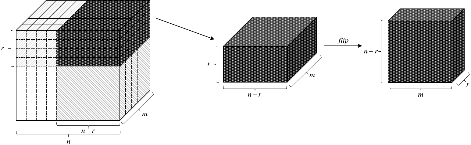
Figure 1: The $3$-tensor $\mathbf{G}$, and flipping $\mathbf{B}^{\prime}$ to get $\mathbf{B}$.

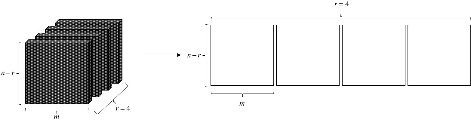
Figure 2: Slicing $\mathbf{B}$.

Define the set of equivalences of $\mathbf{B}$ as $\mathrm{Aut}(\mathbf{B}):=\{(A,D)\in\mathrm{GL}(n-r,q)\times\mathrm{GL}(m,q):\forall i\in[r],AB_{i}D^{-1}=B_{i}\}$. Note that $\mathrm{RAut}(\mathcal{B}^{\prime})$ is the projection of $\mathrm{Aut}(\mathbf{B})$ to the first component. Now define the adjoint algebra of $\mathbf{B}$ as $\mathrm{Adj}(\mathbf{B}):=\{(A,D)\in M(n-r,q)\oplus M(m,q):\forall i\in[r],AB_{i}=B_{i}D\}$. $(A,D)\in M(n-r,q)\oplus M(m,q)$ is called invertible, if both $A$ and $D$ are invertible. Clearly, $\mathrm{Aut}(\mathbf{B})$ consists of the invertible elements in $\mathrm{Adj}(\mathbf{B})$. When $r=4$, $m=n-r=n-4$, it can be shown that the adjoint algebra of $4$ random matrices in $M(m,q)$ is of size $q^{O(m)}$ with probability $1-1/q^{\Omega(m)}$. The key to prove this statement is the stable notion from geometric invariant theory [MFK94] in the context of the left-right action of $\mathrm{GL}(m,q)\times\mathrm{GL}(m,q)$ on matrix tuples $M(m,q)^{r}$. In this context, a matrix tuple $(B_{1},\dots,B_{r})\in M(m,q)^{r}$ is stable, if for every nontrivial subspace $U\leq\mathbb{F}_{q}^{n}$, $\dim(\langle\cup_{i\in[r]}B_{i}(U)\rangle)>\dim(U)$. An upper bound on $|\mathrm{Adj}(\mathbf{B})|$ can be obtained by analysing this notion using some classical algebraic results and elementary probability calculations. The good property we impose on $\mathcal{G}$ is then that the corresponding $|\mathrm{Adj}(\mathbf{B})|\leq q^{O(m)}$. It can be verified that this property does not depend on the choices of bases of $\mathcal{G}$. There is one subtle point though: the analysis on $\mathrm{Adj}(\mathbf{B})$ is done for $4$ random matrices but we want an analysis for $\mathcal{G}$ in the linear algebraic Erdős-Rényi model. This can be fixed by defining a so-called naive model and analysing the relation between the naive model and the LinER model (Section 5).

Now that we have achieved our first goal, namely defining a good property satisfied by most $\mathcal{G}$’s, let us see how this property enables an algorithm for such $\mathcal{G}$’s. For an arbitrary $\mathcal{H}\leq\Lambda(n,q)$, at a multiplicative cost of $q^{O(n)}$ (recall thar $r=4$) we can enumerate all $r$-individualisations. Consider a fixed one, say $\mathbb{F}_{q}^{n}=L\oplus R$ with an ordered basis $(v_{1},\dots,v_{r})$ of $L$. Analogous to the above, we can construct $\mathbf{C}^{\prime}$, flip to get $\mathbf{C}$, and slice $\mathbf{C}$ into $r$ $m\times m$ matrices $(C_{1},\dots,C_{r})$. The task then becomes to compute $\mathrm{Adj}(\mathbf{B},\mathbf{C}):=\{(A,D)\in M(n-r,q)\oplus M(m,q):\forall i\in[r],AB_{i}=C_{i}D\}$. Viewing $A$ and $D$ as variable matrices, $AB_{i}=C_{i}D$ are linear equations on $A$ and $D$, so the solution set can be computed efficiently. As $|\mathrm{Adj}(\mathbf{B})|\leq q^{O(m)}$, for $\mathrm{Adj}(\mathbf{B},\mathbf{C})$ to contain an invertible element, it must be that $|\mathrm{Adj}(\mathbf{B},\mathbf{C})|=|\mathrm{Adj}(\mathbf{B})|\leq q^{O(m)}$. In this case all elements in $\mathrm{Adj}(\mathbf{B},\mathbf{C})$ can be enumerated in time $q^{O(m)}=q^{O(n)}$. For each element $(A,D)\in\mathrm{Adj}(\mathbf{B},\mathbf{C})$, test whether it is invertible, and if so, test whether the $A$ in that solution induces an isometry together with the individualisation. This completes a high-level description of the algorithm. In particular, this implies that if $\mathcal{G}$ satisfies this property, then $|\mathrm{Aut}(\mathcal{G})|\leq q^{O(n)}$. A detailed presentation is in Section 6, which have some minor differences with the outline here, as we want to reduce some technical details.

3 Preliminaries

We collect some notation used in this paper. $q$ is reserved for prime powers, and $p$ for primes. For $n\in\mathbb{N}$, $[n]:=\{1,\dots,n\}$. $\mathbb{F}_{q}$ denotes the field of size $q$. $\mathbf{0}$ denotes the zero vector or the zero vector space. For $i\in[n]$, $e_{i}$ denotes the $i$th standard basis vector of $\mathbb{F}_{q}^{n}$. For a vector space $V$ and $S\subseteq V$, we use $\langle S\rangle$ to denote the linear span of $S$ in $V$. $M(s\times t,q)$ denotes the linear space of matrices of size $s\times t$ over $\mathbb{F}_{q}$, and $M(s,q):=M(s\times s,q)$. $I_{s}$ denotes the $s\times s$ identity matrix. For $A\in M(s\times t,q)$, ${A}^{\mathrm{t}}$ denotes the transpose of $A$. $\mathrm{GL}(n,q)$ is the general linear group consisting of $n\times n$ invertible matrices over $\mathbb{F}_{q}$. $\Lambda(n,q)$ is the linear space of alternating matrices of size $n\times n$ over $\mathbb{F}_{q}$. We use ${\genfrac{[}{]}{0.0pt}{}{\ }{\ }}_{q}$ for the Gaussian binomial coefficient with base $q$, and $\binom{\ }{\ }$ for the ordinary binomial coefficient. For $N\in\mathbb{N}$ and $m\in[N]$, ${\genfrac{[}{]}{0.0pt}{}{N}{m}}_{q}$ counts the number of dimension-$m$ subspaces in $\mathbb{F}_{q}^{N}$.

By a random vector in $\mathbb{F}_{q}^{N}$, we mean a vector of length $N$ where each entry is chosen independently and uniformly random from $\mathbb{F}_{q}$. By a random matrix in $M(s\times t,q)$, we mean a matrix of size $s\times t$ where each entry is chosen independently and uniformly random from $\mathbb{F}_{q}$. By a random alternating matrix in $\Lambda(n,q)$, we mean an alternating matrix of size $n$ where each entry in the strictly upper triangular part is chosen independently and uniformly random from $\mathbb{F}_{q}$. Then the diagonal entries are set to $0$, and the lower triangular entries are set in accordance with the corresponding upper triangular ones.

Fact 4.

Let $N\in\mathbb{N}$ and $m\in\mathbb{N}$ such that $0\leq m\leq N$.

1. For a fixed subspace $U$ in $\mathbb{F}_{q}^{N}$ of dimension $m$, the number of complements of $U$ in $\mathbb{F}_{q}^{N}$ is $q^{m(N-m)}$;

2. A random matrix $A\in M(N\times m,q)$ is of rank $m$ with probability $\geq 1-m/q^{N-m+1}$;

3. A random matrix $A\in M(N\times m,q)$ is of rank $m$ with probability $>1/4$.

Proof.

(1) is well-known. For (2), observe that

$$\Pr[\mathrm{rk}(A)=m|A\in M(N\times m,q)] = (1-1/q^{N})(1-1/q^{N-1})\dots(1-1/q^{N-m+1})$$

$$\geq 1-(1/q^{N}+1/q^{N-1}+\dots+1/q^{N-m+1})$$

$$\geq 1-m/q^{N-m+1}.$$

For (3), this is because $\frac{1}{2}\cdot\frac{3}{4}\cdot\frac{7}{8}\cdot\dots\approx 0.288788>1/4$. ∎

4 Matrix tuples and matrix spaces

An $r$-matrix tuple of size $s\times t$ over $\mathbb{F}_{q}$ is an element in $M(s\times t,q)^{r}$. An $r$-matrix space of size $s\times t$ over $\mathbb{F}_{q}$ is a dimension-$r$ subspace in $M(s\times t,q)$. An $m$-alternating (matrix) tuple of size $n$ over $\mathbb{F}_{q}$ is an element from $\Lambda(n,q)^{m}$. An $m$-alternating (matrix) space of size $n$ over $\mathbb{F}_{q}$ is a dimension-$m$ subspace in $\Lambda(n,q)$. In the rest of this article we let $N_{n}=\binom{n}{2}=\dim(\Lambda(n,q))$, or just $N$ if $n$ is obvious from the context.

We shall use $\mathcal{G}$, $\mathcal{H}$, …, to denote alternating spaces, and $\mathbf{G}$, $\mathbf{H}$, …, to denote alternating tuples. $\mathcal{B}$, $\mathcal{C}$, …, are for (not necessarily alternating nor square) matrix spaces, and $\mathbf{B}$, $\mathbf{C}$ for (not necessarily alternating nor square) matrix tuples. We say that a matrix tuple $\mathbf{B}$ represents a matrix space $\mathcal{B}$, if the matrices in $\mathbf{B}$ form a spanning set (not necessarily a basis) of $\mathcal{B}$. Given $A\in M(s,q)$, $D\in M(t,q)$, and $\mathbf{B}=(B_{1},\dots,B_{r})\in M(s\times t,q)^{r}$, $A\mathbf{B}D$ is the tuple $(AB_{1}D,\dots,AB_{r}D)$. For $Z=(z_{i,j})\in M(r,q)$, $\mathbf{B}^{Z}=(\sum_{i\in[r]}z_{1,i}B_{i},\sum_{i\in[r]}z_{2,i}B_{i},\dots,\sum_{i\in[r]}z_{r,i}B_{i})$.

Two alternating tuples $\mathbf{G}=(G_{1},\dots,G_{m})$ and $\mathbf{H}=(H_{1},\dots,H_{m})$ in $\Lambda(n,q)^{m}$ are isometric, if there exists $A\in\mathrm{GL}(n,q)$, ${A}^{\mathrm{t}}\mathbf{G}A=\mathbf{H}$. Two alternating spaces $\mathcal{G}$ and $\mathcal{H}$ in $\Lambda(n,q)$ are isometric, if there exists $A\in\mathrm{GL}(n,q)$, such that ${A}^{\mathrm{t}}\mathcal{G}A=\mathcal{H}$ (equal as subspaces). Given alternating tuples $\mathbf{G}\in\Lambda(n,q)^{m}$ and $\mathbf{H}\in\Lambda(n,q)^{m}$ representing $\mathcal{G}$ and $\mathcal{H}$ respectively, $\mathcal{G}$ and $\mathcal{H}$ are isometric, if and only if there exists $Z\in\mathrm{GL}(m,q)$ such that $\mathbf{G}$ and $\mathbf{H}^{Z}$ are isometric – in other words, there exist $A\in\mathrm{GL}(n,q)$ and $Z\in\mathrm{GL}(m,q)$, such that ${A}^{\mathrm{t}}\mathbf{G}A=\mathbf{H}^{Z}$. We use $\mathrm{Iso}(\mathcal{G},\mathcal{H})\subseteq\mathrm{GL}(n,q)$ to denote the set of isometries between $\mathcal{G}$ and $\mathcal{H}$. When $\mathcal{G}=\mathcal{H}$, the isometries between $\mathcal{G}$ and $\mathcal{G}$ are also called autometries. The set of all autometries forms a matrix group, and let $\mathrm{Aut}(\mathcal{G})=\mathrm{Iso}(\mathcal{G},\mathcal{G})\leq\mathrm{GL}(n,q)$. $\mathrm{Iso}(\mathcal{G},\mathcal{H})$ is either empty or a right coset w.r.t. $\mathrm{Aut}(\mathcal{G})$. Analogously, we can define the corresponding concepts for tuples $\mathrm{Iso}(\mathbf{G},\mathbf{H})$ and $\mathrm{Aut}(\mathbf{G})$.

Two matrix tuples $\mathbf{B}=(B_{1},\dots,B_{r})$ and $\mathbf{C}=(C_{1},\dots,C_{r})$ in $M(s\times t,q)^{r}$ are equivalent, if there exist $A\in\mathrm{GL}(s,q)$ and $D\in\mathrm{GL}(t,q)$, such that $A\mathbf{B}D^{-1}=\mathbf{C}$. Two matrix spaces $\mathcal{B}$ and $\mathcal{C}$ in $M(s\times t,q)$ are equivalent, if there exist $A\in\mathrm{GL}(s,q)$ and $D\in\mathrm{GL}(t,q)$, such that $A\mathcal{B}D^{-1}=\mathcal{C}$ (equal as subspaces). By abuse of notation, we use $\mathrm{Iso}(\mathcal{B},\mathcal{C})\leq\mathrm{GL}(s,q)\times\mathrm{GL}(t,q)$ to denote the set of equivalences between $\mathcal{B}$ and $\mathcal{C}$, and let $\mathrm{Aut}(\mathcal{B})=\mathrm{Iso}(\mathcal{B},\mathcal{B})$. $\mathrm{Iso}(\mathcal{B},\mathcal{C})$ is either empty or a left coset of $\mathrm{Aut}(\mathcal{B})$. Similarly we have $\mathrm{Iso}(\mathbf{B},\mathbf{C})$ and $\mathrm{Aut}(\mathbf{B})$. A trivial but useful observation is that $\mathrm{Iso}(\mathbf{B},\mathbf{C})$ and $\mathrm{Aut}(\mathbf{B})$ are naturally contained in certain subspaces of $M(s,q)\oplus M(t,q)$ as follows. Following [Wil09], we define the adjoint algebra of $\mathbf{B}\in M(s\times t,q)^{r}$ as $\mathrm{Adj}(\mathbf{B})=\{(A,D)\in M(s,q)\oplus M(t,q):A\mathbf{B}=\mathbf{B}D\}$. This is a classical concept, and is recently studied in the context of $p$-group isomorphism testing by Wilson et al. [Wil09, LW12, BW12, BMW15]. We further define the adjoint space between $\mathbf{B}$ and $\mathbf{C}$ in $M(s\times t,q)^{r}$ as $\mathrm{Adj}(\mathbf{B},\mathbf{C})=\{(A,D)\in M(s,q)\oplus M(t,q):A\mathbf{B}=\mathbf{C}D\}$. $(A,D)\in M(s,q)\oplus M(t,q)$ is called invertible if both $A$ and $D$ are invertible. Then $\mathrm{Aut}(\mathbf{B})$ (resp. $\mathrm{Iso}(\mathbf{B},\mathbf{C})$) consists of invertible elements in $\mathrm{Adj}(\mathbf{B})$ (resp. $\mathrm{Adj}(\mathbf{B},\mathbf{C})$). An easy observation is that if $\mathbf{B}$ and $\mathbf{C}$ are isometric, then an isometry defines a bijection between $\mathrm{Adj}(\mathbf{B},\mathbf{C})$ and $\mathrm{Adj}(\mathbf{B})$.

Given $\mathbf{B}=(B_{1},\dots,B_{r})\in M(s\times t,q)^{r}$, let $\mathrm{im}(\mathbf{B})=\langle\cup_{i\in[m]}\mathrm{im}(B_{i})\rangle$ and $\ker(\mathbf{B})=\cap_{i\in[m]}\ker(B_{i})$. $\mathbf{B}$ is image-nondegenerate (resp. kernel-nondegenerate), if $\mathrm{im}(\mathbf{B})=\mathbb{F}_{q}^{s}$ (resp. $\ker(\mathbf{B})=\mathbf{0}$). Note that if $\mathbf{B}$ is an alternating tuple in $\Lambda(n,q)^{m}$, then $\mathbf{B}$ is image-nondegenerate if and only if it is kernel-nondegenerate, as $\mathrm{im}(\mathbf{B})$ and $\ker(\mathbf{B})$ are orthogonal to each other w.r.t. the standard bilinear form on $\mathbb{F}_{q}^{n}$. $\mathbf{B}$ is nondegenerate if it is both image-nondegenerate and kernel-nondegenerate. If $\mathbf{B}$ is image-nondegenerate (resp. kernel-nondegenerate), then the projection of $\mathrm{Adj}(\mathbf{B})$ to the first (resp. second) component along the second (resp. the first) component is injective.

For a matrix tuple $\mathbf{B}=(B_{1},\dots,B_{r})\in M(s\times t,q)^{r}$ and a subspace $U\leq\mathbb{F}_{q}^{t}$, the image of $U$ under $\mathbf{B}$ is $\mathbf{B}(U):=\langle\cup_{i\in[m]}B_{i}(U)\rangle$. It is easy to verify that, $(A\mathbf{B})(U)=A(\mathbf{B}(U))$, and $(\mathbf{B}D)(U)=(\mathbf{B}(D(U)))$. $U\leq\mathbb{F}_{q}^{t}$ is trivial if $U=\mathbf{0}$ or $U=\mathbb{F}_{q}^{t}$.

Definition 5.

$\mathbf{B}\in M(s\times t,q)^{r}$ is stable, if $\mathbf{B}$ is nondegenerate, and for every nontrivial subspace $U\leq\mathbb{F}_{q}^{t}$, $\dim(\mathbf{B}(U))/\dim(U)>s/t$.

Remark 6.

In Definition 5, we can replace nondegenerate with image-nondegenerate, as the second condition already implies kernel-nondegenerate.

Lemma 7, 9 and Claim 11 are classical and certainly known to experts. However for completeness we include proofs which may be difficult to extract from the literature.

Lemma 7.

If $\mathbf{B}$ is stable, then any nonzero $(A,D)\in\mathrm{Adj}(\mathbf{B})$ is invertible.

Proof.

Take any $(A,D)\in\mathrm{Adj}(\mathbf{B})$. If $D=0$, then $A\mathbf{B}=\mathbf{B}D=0$, and by the image nondegeneracy of $\mathbf{B}$, $A$ has to be $0$.

Suppose now that $D$ is not invertible nor $0$, so $\ker(D)$ is not $\mathbf{0}$ nor $\mathbb{F}_{q}^{t}$. By $A\mathbf{B}(\ker(D))=\mathbf{B}D(\ker(D))=0$, $A(\mathbf{B}(\ker(D)))=0$, which gives $\ker(A)\geq\mathbf{B}(\ker(D))$. As $\mathbf{B}$ is stable, we have $\dim(\mathbf{B}(\ker(D)))>(s/t)\dim(\ker(D))$, so $\dim(\ker(A))>(s/t)\dim(\ker(D))$. On the other hand, $A\mathbf{B}(\mathbb{F}_{q}^{t})=\mathbf{B}D(\mathbb{F}_{q}^{t})$. Again, by the image nondegeneracy of $\mathbf{B}$, $\mathbf{B}(\mathbb{F}_{q}^{t})=\mathbb{F}_{q}^{s}$, so $A\mathbf{B}(\mathbb{F}_{q}^{t})=\mathrm{im}(A)$, and we see that $\mathrm{im}(A)=\mathbf{B}(\mathrm{im}(D))$. As $\mathbf{B}$ is stable, $\dim(\mathrm{im}(A))>(s/t)\dim(\mathrm{im}(D))$. It follows that $s=\dim(\mathrm{im}(A))+\dim(\ker(A))>(s/t)(\dim(\mathrm{im}(D))+\dim(\ker(D)))=(s/t)\cdot t=s$. This is a contradiction, so $D$ has to be invertible.

If $D$ is invertible, then $\mathbf{B}D$ is image-nondegenerate, so $A$ has to be invertible, as otherwise $A\mathbf{B}$ would not be image-nondegenerate. ∎

Remark 8.

We present some background information on the stable concept and Lemma 7, for readers who have not encountered these before. Briefly speaking, the stable concept is a correspondence of the concept of simple as in representation theory of associative algebras, and Lemma 7 is an analogue of the Schur’s lemma there. Both the stable concept here and the simple concept are special cases of the stable concept in geometric invariant theory [MFK94, Kin94], specialised to the left-right action of $\mathrm{GL}(s,q)\times\mathrm{GL}(t,q)$ on $M(s\times t,q)^{r}$, and the conjugation action of $\mathrm{GL}(s,q)$ on $M(s,q)^{r}$, respectively.

Specifically, consider a tuple of square matrices $\mathbf{B}\in M(s,q)^{r}$, which can be understood as a representation of an associative algebra with $r$ generators. This representation is simple if and only if it does not have a non-trivial invariant subspace, that is $U\leq\mathbb{F}_{q}^{s}$, such that $\mathbf{B}(U)\leq U$. This amounts to say that there does not exist $A\in\mathrm{GL}(s,q)$ such that every $B$ in $A\mathbf{B}A^{-1}$ is in the form $\begin{bmatrix}B_{1}&B_{2}\\ 0&B_{3}\end{bmatrix}$ where $B_{i}\in M(s^{\prime},q)$, $1\leq s^{\prime}\leq s-1$. On the other hand, the stable concept can be rephrased as the following. $\mathbf{B}\in M(s\times t,q)^{r}$ is stable, if there do not exist $A\in\mathrm{GL}(s,q)$ and $D\in\mathrm{GL}(t,q)$ such that every $B\in A\mathbf{B}D^{-1}$ is of the form $\begin{bmatrix}B_{1}&B_{2}\\ 0&B_{3}\end{bmatrix}$ where $B_{1}$ is of size $s^{\prime}\times t^{\prime}$, $1\leq t^{\prime}\leq t-1$, such that $s^{\prime}/t^{\prime}\leq s/t$.

Lemma 7 can be understood as an analogue of Schur’s lemma, which states that if $\mathbf{B}\in M(s,q)^{r}$ is simple then a nonzero homomorphism $A\in M(s,q)$ of $\mathbf{B}$ (e.g. $A\mathbf{B}A^{-1}=\mathbf{B}$) has to be invertible.

The proof of the following classical result was communicated to us by G. Ivanyos.

Lemma 9.

Let $\mathfrak{A}\subseteq M(n,q)$ be a field containing $\lambda I_{n}$, $\lambda\in\mathbb{F}_{q}$. Then $|\mathfrak{A}|\leq q^{n}$.

Proof.

$\mathfrak{A}$ is an extension field of $\mathbb{F}_{q}$, and suppose its extension degree is $d$. Then $\mathbb{F}_{q}^{n}$ is an $\mathfrak{A}$-module, or in other words, a vector space over $\mathfrak{A}$. So $\mathbb{F}_{q}^{n}\cong\mathfrak{A}^{m}$ as vector spaces over $\mathfrak{A}$ for some $m\in\mathbb{N}$. Considering them as $\mathbb{F}_{q}$ vector spaces, we have $n=md$ so $d$ divides $n$. It follows that $|\mathfrak{A}|=q^{d}\leq q^{n}$. ∎

By Lemma 7 and 9, we have the following.

Proposition 10.

If $\mathbf{B}\leq M(s\times t,q)^{r}$ is stable, then $|\mathrm{Adj}(\mathbf{B})|\leq q^{s}$.

Proof.

As $\mathbf{B}$ is stable, it is nondegenerate, so the projection of $\mathrm{Adj}(\mathbf{B})\leq M(s,q)\oplus M(t,q)$ to $M(s,q)$ (naturally embedded in $M(s,q)\oplus M(t,q)$) along $M(t,q)$ is injective. By Lemma 7, the image of the projection is a finite division algebra over $\mathbb{F}_{q}$ containing $\lambda I$. So by Wedderburn’s little theorem, it is a field. By Lemma 9, the result follows. ∎

Let us also mention an easy property about stable.

Claim 11.

Given $\mathbf{B}=(B_{1},\dots,B_{r})\in M(s\times t,q)^{r}$, let ${\mathbf{B}}^{\mathrm{t}}=({B}^{\mathrm{t}}_{1},\dots,{B}^{\mathrm{t}}_{r})\in M(t\times s,q)^{r}$. Then $\mathbf{B}$ is stable if and only if ${\mathbf{B}}^{\mathrm{t}}$ is stable.

Proof.

First we consider the nondegenerate part. If $u\in\mathbb{F}_{q}^{s}$ satisfies $\mathbf{B}(u)=\mathbf{0}$, then it is easy to verify that ${\mathbf{B}}^{\mathrm{t}}(\mathbb{F}_{q}^{t})$ is contained in the hyperplane defined by $u$, e.g. ${u}^{\mathrm{t}}({\mathbf{B}}^{\mathrm{t}}(\mathbb{F}_{q}^{s}))=0$. If $\mathbf{B}(\mathbb{F}_{q}^{t})\neq\mathbb{F}_{q}^{s}$, then there exists some $u\in\mathbb{F}_{q}^{s}$ such that ${u}^{\mathrm{t}}(\mathbf{B}(\mathbb{F}_{q}^{t}))=0$, so $u\in\ker({\mathbf{B}}^{\mathrm{t}})$. Therefore $\mathbf{B}$ is nondegenerate if and only if ${\mathbf{B}}^{\mathrm{t}}$ is nondegenerate.

In the following we assume that $\mathbf{B}$ is nondegenerate, and check nontrivial subspaces to show that $\mathbf{B}$ is not stable if and only if ${\mathbf{B}}^{\mathrm{t}}$ is not stable. This can be seen easily from the discussion in Remark 8. $\mathbf{B}$ is not stable, then there exist $A\in\mathrm{GL}(r,q)$ and $D\in\mathrm{GL}(t,q)$ such that every $B\in A\mathbf{B}D^{-1}$ is of the form $\begin{bmatrix}B_{1}&B_{2}\\ 0&B_{3}\end{bmatrix}$ where $B_{1}$ is of size $s^{\prime}\times t^{\prime}$, $1\leq t^{\prime}\leq t-1$, such that $s^{\prime}/t^{\prime}\leq s/t$. Note that $s^{\prime}>0$ as otherwise $\mathbf{B}$ is degenerate, so $1\leq s^{\prime}\leq\frac{s}{t}\cdot t^{\prime}<s$. Now consider $D^{-\mathrm{t}}{\mathbf{B}}^{\mathrm{t}}{A}^{\mathrm{t}}$, the elements in which is of the form $\begin{bmatrix}{B}^{\mathrm{t}}_{1}&0\\ {B}^{\mathrm{t}}_{2}&{B}^{\mathrm{t}}_{3}\end{bmatrix}$. Note that ${B}^{\mathrm{t}}_{3}$ is of size $(t-t^{\prime})\times(s-s^{\prime})$ where $1\leq s-s^{\prime}\leq s-1$, $1\leq t-t^{\prime}\leq t-1$, and $(t-t^{\prime})/(s-s^{\prime})\leq t/s$ (by $s^{\prime}/t^{\prime}\leq s/t$). It follows that $D^{-\mathrm{t}}{\mathbf{B}}^{\mathrm{t}}{A}^{\mathrm{t}}$ is not stable, so ${\mathbf{B}}^{\mathrm{t}}$ is not stable. This concludes the proof. ∎

5 Random alternating matrix spaces

For $n\in\mathbb{N}$, $N=\binom{n}{2}$. Recall the definition of the linear algebraic Erdős-Rényi model, $\mbox{\sc LinER}(n,m)$ in Model 1. It turns out for our purpose, we can work with the following model.

Model 3 (Naive models for matrix tuples and matrix spaces).

The naive model for alternating tuples, $\mbox{\sc NaiT}(n,m,q)$, is the probability distribution over the set of all $m$-tuples of $n\times n$ alternating tuples, where each tuple is endowed with probability $1/q^{Nm}$.

The naive model for alternating spaces, $\mbox{\sc NaiS}(n,m,q)$, is the probability distribution over the set of alternating spaces in $\Lambda(n,q)$ of dimension $\leq m$, where the probability at some $\mathcal{G}\leq\Lambda(n,q)$ of dimension $0\leq d\leq m$ equals the number of $m$-tuples of $n\times n$ alternating tuples that represent $\mathcal{G}$, divided by $q^{Nm}$.

While we aim at analysing the algorithm in the LinER model, we will ultimately work with the naive model due to its simplicity, as it is just an $m$-tuple of random $n\times n$ alternating matrices. The naive model for alternating spaces, NaiS, then is obtained by taking the linear spans of such tuples. The following observation will be useful.

Observation 12.

Every $m$-alternating space has $(q^{m}-1)(q^{m}-q)\dots(q^{m}-q^{m-1})$ $m$-alternating tuples representing it.

We now justify that working with the naive model suffices for the analysis even in the linear algebraic Erdős-Rényi model. Consider the following setting. Suppose we have $E(n,m,q)$, a property of dimension-$m$ alternating spaces in $\Lambda(n,q)$, and wish to show that $E(n,m,q)$ holds with high probability in $\mbox{\sc LinER}(n,m,q)$. $E(n,m,q)$ naturally induces $E^{\prime}(n,m,q)$, a property of alternating tuples in $\Lambda(n,q)^{m}$ that span dimension-$m$ alternating spaces. It is usually the case that there exists a property $F(n,m,q)$ of all $m$-alternating tuples in $\Lambda(n,q)^{m}$, so that $F(n,m,q)$ and $E^{\prime}(n,m,q)$ coincide when restricting to those alternating tuples spanning dimension-$m$ matrix spaces. If we could prove that $F(n,m,q)$ holds with high probability, then since a nontrivial fraction of $m$-tuples do span dimension-$m$ spaces, we would get that $E(n,m,q)$ holds with high probability as well. The following proposition summarises and makes precise the above discussion.

Proposition 13.

Let $E(n,m,q)$ and $F(n,m,q)$ be as above. Suppose in $\mbox{\sc NaiT}(n,m,q)$, $F(n,m,q)$ happens with probability $\geq 1-f(n,m,q)$ where $0\leq f(n,m,q)<1$. Then in $\mbox{\sc LinER}(n,m,q)$, $E(n,m,q)$ happens with probability $>1-4\cdot f(n,m,q)$.

Proof.

The number of tuples for which $F(n,m,q)$ fails is no larger than $f(n,m,q)\cdot q^{Nm}$. Clearly the bad situation for $E^{\prime}(n,m,q)$ is when each of them spans an $m$-alternating space, so we focus on this case. Recall that $E^{\prime}(n,m,q)$ is induced from a property of $m$-alternating spaces. That is, if two tuples span the same $m$-alternating space, then either both of them satisfy $E^{\prime}(n,m,q)$, or neither of them satisfies $E^{\prime}(n,m,q)$. By Observation 12, the number of $m$-alternating spaces for which $E(n,m,q)$ fails is $\leq f(n,m,q)\cdot\frac{q^{Nm}}{(q^{m}-1)(q^{m}-q)\dots(q^{m}-q^{m-1})}$. The fraction of $m$-alternating spaces for which $E(n,m,q)$ fails is then $\leq f(n,m,q)\cdot\frac{q^{Nm}}{(q^{N}-1)(q^{N}-q)\dots(q^{N}-q^{N-m+1})}<4\cdot f(n,m,q)$ where $4$ comes from Fact 4 (3). ∎

5.1 Random matrix spaces

For $s,t,r\in\mathbb{Z}^{+}$, we can define the Erdős-Rényi model for bipartite graphs on the vertex set $[s]\times[t]$ with edge set size $r$ by taking every subset of $[s]\times[t]$ of size $r$ with probability $\binom{st}{r}$. Analogously we can define the following in the matrix space setting.

1. The bipartite linear algebraic Erdős-Rényi model $\mbox{\sc BipLinER}(s\times t,r,q)$: each $r$-matrix space in $M(s\times t,q)$ is chosen with probability $1/{\genfrac{[}{]}{0.0pt}{}{st}{r}}_{q}$.

2. The bipartite naive model $\mbox{\sc BipNaiT}(s\times t,r,q)$ for matrix tuples: each $r$-matrix tuple in $M(s\times t,q)^{r}$ is chosen with probability $1/q^{str}$.

3. The bipartite naive model $\mbox{\sc BipNaiS}(s\times t,r,q)$ for matrix spaces: each matrix space $\mathcal{B}$ of dimension $d$, $0\leq d\leq r$ in $M(s\times t,q)$, is chosen with probability $a/q^{str}$ where $a$ is the number of $r$-matrix tuples representing $\mathcal{B}$.

6 The main algorithm

We will first define the property $F(n,m,q,r)$ for the average-case analysis in Section 6.1. To lower bound the probability of $F(n,m,q,r)$ we will actually work with a stronger property $F^{\prime}(n,m,q,r)$ in Section 6.1.1. Given this property we describe and analyse the main algorithm in Section 6.2. It should be noted that the algorithm here differs slightly from the outline from Section 2.3, as there we wanted to reduce some technical details.

6.1 Some properties of alternating spaces and alternating tuples

An $m$-alternating space $\mathcal{G}\leq\Lambda(n,q)$ induces $\mathcal{B}^{\prime}=\{[e_{1},\dots,e_{r}]^{t}G[e_{r+1},\dots,e_{n}]:G\in\mathcal{G}\}$ which is a matrix space in $M(r\times(n-r),q)$ of dimension no more than $m$. Define $\mathrm{RAut}(\mathcal{B}^{\prime}):=\{A\in\mathrm{GL}(n-r,q):\mathcal{B}^{\prime}A=\mathcal{B}^{\prime}\}$. An element in $\mathrm{RAut}(\mathcal{B}^{\prime})$ is called a right-side equivalence of $\mathcal{B}^{\prime}$.

Definition 14.

$E^{\prime}(n,m,q,r)$ is a property of $m$-alternating spaces in $\Lambda(n,q)$, defined as follows. Given an $m$-alternating space $\mathcal{G}$ in $\Lambda(n,q)$, let $\mathcal{B}^{\prime}$ be the matrix space in $M(r\times(n-r),q)$ defined as above. $\mathcal{G}$ belongs to $E^{\prime}(n,m,q,r)$, if and only if $|\mathrm{RAut}(\mathcal{B}^{\prime})|\leq q^{n-r}$.

Right-side equivalence is a useful concept that leads to our algorithm (as seen in Section 2.2), but what we actually need is the following linearisation of $\mathrm{RAut}(\mathcal{B}^{\prime})$.

Definition 15.

$E(n,m,q,r)$ is a property of $m$-alternating spaces in $\Lambda(n,q)$, defined as follows. Given an $m$-alternating space $\mathcal{G}$ in $\Lambda(n,q)$, let $\mathcal{B}^{\prime}$ be the matrix space in $M(r\times(n-r),q)$ defined as above. $\mathcal{G}$ belongs to $E(n,m,q,r)$, if and only if $|\{A\in M(n-r,q):\mathcal{B}^{\prime}A\leq\mathcal{B}^{\prime}\}|\leq q^{n-r}$.

We define a property $F(n,m,q,r)$ for alternating tuples that corresponds to $E(n,m,q,r)$. Given $\mathbf{G}=(G_{1},\dots,G_{m})\in\Lambda(n,q)^{m}$, we can construct a matrix tuple $\mathbf{B}^{\prime}=([e_{1},\dots,e_{r}]^{t}B_{1}[e_{r+1},\dots,e_{n}],\dots,$ $[e_{1},\dots,e_{r}]^{t}B_{m}[e_{r+1},\dots,e_{n}])$ in $M(r\times(n-r),q)^{m}$.

Definition 16.

$F(n,m,q,r)$ is a property of $m$-alternating tuples in $\Lambda(n,q)^{m}$, defined as follows. Given an $m$-alternating tuple $\mathbf{G}$ in $\Lambda(n,q)^{m}$, let $\mathbf{B}^{\prime}$ be the $m$-matrix tuple in $M(r\times(n-r),q)^{m}$ defined as above. $\mathbf{G}$ belongs to $E(n,m,q,r)$, if and only if $|\{A\in M(n-r,q):~{}\exists D\in M(m,q),~{}\mathbf{B}^{\prime}A=\mathbf{B}^{\prime D}\}|\leq q^{n-r}$.

It is not hard to see that $F(n,m,q,r)$ is a proper extension of $E(n,m,q,r)$.

Proposition 17.

Suppose $\mathbf{G}\in\Lambda(n,q)^{m}$ represents an $m$-alternating space $\mathcal{G}\leq\Lambda(n,q)$. Then $\mathbf{G}$ is in $F(n,m,q,r)$ if and only if $\mathcal{G}$ is in $E(n,m,q,r)$.

Proof.

Let $\mathcal{B}^{\prime}$ and $\mathbf{B}^{\prime}$ be the matrix space and matrix tuple defined as above for $\mathcal{G}$ and $\mathbf{G}$, respectively. Clearly $\mathbf{B}^{\prime}$ represents $\mathcal{B}^{\prime}$, so $\mathbf{B}^{\prime}A$ represents $\mathcal{B}^{\prime}A$. Finally note that $\mathbf{B}^{\prime}A=\mathbf{B}^{\prime D}$ for some $D\in M(n,q)$ if and only if the linear span of $\mathbf{B}^{\prime}A$ is contained in the linear span of $\mathbf{B}^{\prime}$, that is $\mathcal{B}^{\prime}A\leq\mathcal{B}^{\prime}$. ∎

Instead of working with $\mathbf{B}^{\prime}$ and $\{A\in\mathrm{GL}(n-r,q):\exists D\in\mathrm{GL}(m,q),\mathbf{B}^{\prime}A=\mathbf{B}^{\prime D}\}$, it is more convenient to flip $\mathbf{B}^{\prime}$, an $m$-matrix tuple of size $r\times(n-r)$, to get $\mathbf{B}$, an $r$-matrix tuple of size $(n-r)\times m$. Then $\{A\in M(n-r,q):\exists D\in M(m,q),\mathbf{B}^{\prime}A=\mathbf{B}^{\prime D}\}=\{A\in M(n-r,q):\exists D\in M(m,q),A\mathbf{B}=\mathbf{B}D\}$. The latter is closely related to the adjoint algebra concept for matrix tuples as defined in Section 4. Recall that $\mathrm{Adj}(\mathbf{B})=\{(A,D)\in M(n-r,q)\oplus M(m,q):A\mathbf{B}=\mathbf{B}D\}$. Let $\pi_{1}:M(n-r,q)\oplus M(m,q)\to M(n-r,q)$ be the projection to the first component along the second. $\{A\in M(n-r,q):\exists D\in M(m,q),A\mathbf{B}=\mathbf{B}D\}$ is then just $\pi_{1}(\mathrm{Adj}(\mathbf{B}))$. So Definition 16 is equivalent to the following.

Definition 16, alternative formulation. $F(n,m,q,r)$ is a property of $m$-alternating tuples in $\Lambda(n,q)^{m}$, defined as follows. Given an $m$-alternating tuple $\mathbf{G}$ in $\Lambda(n,q)^{m}$, let $\mathbf{B}$ be the $m$-matrix tuple in $M((n-r)\times m,q)^{r}$ defined as above. $\mathbf{G}$ belongs to $E(n,m,q,r)$, if and only if $|\pi_{1}(\mathrm{Adj}(\mathbf{B}))|\leq q^{n-r}$.

Our algorithm will be based on the property $F(n,m,q,r)$. To show that $F(n,m,q,r)$ holds with high probability though, we turn to study the following stronger property.

Definition 18.

$F^{\prime}(n,m,q,r)$ is a property of $m$-alternating tuples in $\Lambda(n,q)^{m}$, defined as follows. Given an $m$-alternating tuple $\mathbf{G}$ in $\Lambda(n,q)^{m}$, let $\mathbf{B}$ be the $r$-matrix tuple in $M((n-r)\times m,q)^{r}$ defined as above. $\mathbf{G}$ belongs to $F^{\prime}(n,m,q,r)$, if and only if $|\mathrm{Adj}(\mathbf{B})|\leq q^{n-r}$.

Clearly $F^{\prime}(n,m,q,r)$ implies $F(n,m,q,r)$. To show that $F^{\prime}(n,m,q,r)$ holds with high probability, Proposition 10 immediately implies the following, which directs us to make use of the stable property.

Proposition 19.

Let $\mathbf{G}$ and $\mathbf{B}$ be defined as above. If $\mathbf{B}$ is stable, then $\mathbf{G}\in F^{\prime}(n,m,q,r)$.

6.1.1 Estimating the probability for the property $F^{\prime}(n,m,q,r)$

We now show that $F^{\prime}(n,m,q,r)$ holds with high probability, when $m=cn$ for some constant $c$ with an appropriate choice of $r$ depending on $c$. The integer $r$ is chosen so that $r\geq 4\cdot\frac{n-r}{m}$ if $n-r\geq m$, and $r\geq 4\cdot\frac{m}{n-r}$ if $m\geq n-r$. When $n$ is large enough this is always possible. For example, if $c\geq 1$, let $r$ be any integer $\geq 5c$, which ensures that $r\geq 4\cdot\frac{m}{n-r}$ if $n\geq 25c$. If $0<c<1$, let $r$ be an integer $\geq 5/c$. If $n-5/c\geq m$, then $r\geq 5\cdot\frac{n-r}{m}\geq 4\cdot\frac{n-r}{m}$. If $n-5/c<m$, then $r\geq 5\cdot\frac{n-r}{m}\geq 4\cdot\frac{m}{n-r}$ if $n\geq\frac{r}{1-2c/\sqrt{5}}$.

Let $s=n-r$ and $t=m$. By Proposition 19, to show $F^{\prime}(n,m,q,r)$ holds with high probability, we can show that for most $\mathbf{G}$ from $\mbox{\sc NaiT}(n,m,q)$, the corresponding $\mathbf{B}$ in $M(s\times t,q)^{r}$ is stable. A simple observation is that $\mbox{\sc NaiT}(n,m,q)$ induces $\mbox{\sc BipNaiT}(s\times t,r,q)$ obtained by flipping the upper right $s\times t$ corners of the alternating matrices (see Figure 1). So we reduce to estimate the probability of an $r$-matrix tuple $\mathbf{B}$ in $M(s\times t,q)^{r}$ being stable in the model $\mbox{\sc BipNaiT}(s\times t,r,q)$.

By our choice of $r$, we obtain an $r$-matrix tuple $M(s\times t,q)$ with $r\geq 4\cdot\frac{\max(s,t)}{\min(s,t)}$. By Claim 11, we know $\Pr[\mathbf{B}\text{ is stable in }\mbox{\sc BipNaiT}(s\times t,r,q)]=\Pr[\mathbf{C}\text{ is stable in }\mbox{\sc BipNaiT}(t\times s,r,q)]$ via the transpose map. So it is enough to consider the case when $s\geq t$.

Proposition 20.

Give positive integers $s$, $t$, and $r$ such that $s\geq t\geq 16$, $\frac{s}{t}=b\geq 1$, and $r\geq 4\cdot\frac{s}{t}$. Then $\mathbf{B}$ is stable with probability $1-\frac{1}{q^{\Omega(t)}}$ in $\mbox{\sc BipNaiT}(s\times t,r,q)$, where $\Omega(t)$ hides a positive constant depending on $b$.

Proof.

We will upper bound the probability of $\mathbf{B}$ being not stable in $\mbox{\sc BipNaiT}(s\times t,r,q)$, which is

$$P=\Pr[\mathbf{B}~{}\text{is degenerate, or }\exists U\leq\mathbb{F}_{q}^{t},U\text{ non-trivial},\frac{{\dim}(\mathbf{B}(U))}{\dim(U)}\leq\frac{s}{t}].$$

By the union bound, we have:

$$P\leq\sum_{U\leq\mathbb{F}_{q}^{t},1\leq\dim(U)\leq t-1}\Pr[\frac{{\dim}(\mathbf{B}(U))}{\dim(U)}\leq\frac{s}{t}]+\Pr[\mathbf{B}~{}{\rm is~{}degenerate}].$$

About $\mathbf{B}$ being degenerate.

By Remark 6, we only need to bound $\Pr[\mathbf{B}\text{ is image-degenerate}]$. Noticing that $\mathrm{im}(\mathbf{B})$ is spanned by the columns of $B_{i}$’s, by forming an $s\times rt$ matrix $A=[B_{1},B_{2},\dots,B_{r}]$, this amounts to upper bound the probability that $\Pr[\mathrm{rk}(A)<s|A\in M(s\times rt,q)]$. As $rt\geq 4bt=4s$,

$$\Pr[\mathrm{rk}(A)=s|A\in M(s\times rt,q)]\geq\Pr[\mathrm{rk}(A)=s|A\in M(s\times 4s,q)]\geq 1-s/q^{3s+1},$$

where the last inequality is from Fact 4 (2). So we have $\Pr[\mathbf{B}\text{ is image-degenerate}]\leq 1/q^{\Omega(t)}$ since $s=bt$.

Reduce to work with nontrivial subspaces according to the dimension $d$.

Now we focus on $\sum_{U\leq\mathbb{F}_{q}^{t},1\leq\dim(U)\leq t-1}\Pr[\frac{{\dim}(\mathbf{B}(U))}{\dim(U)}\leq\frac{s}{t}]$ in the following. For a nontrivial subspace $U\leq\mathbb{F}_{q}^{t}$, let

$$B_{U}=\{\mathbf{B}\in M(s\times t,q)^{r}:\frac{{\dim}(\mathbf{B}(U))}{\dim(U)}\leq\frac{s}{t}\}.$$

Consider two subspace $U_{1},U_{2}\leq\mathbb{F}_{q}^{t}$ of the same dimension $1\leq d\leq t-1$. We claim that $|B_{U_{1}}|=|B_{U_{2}}|$. Let $X\in\mathrm{GL}(t,q)$ be any invertible matrix such that $X(U_{2})=U_{1}$, and consider the map $T_{X}:M(s\times t,q)^{r}\to M(s\times t,q)^{r}$ defined by sending $\mathbf{B}$ to $\mathbf{B}X$. It is easy to verify that $T_{X}$ is a bijection between $B_{U_{1}}$ and $B_{U_{2}}$. The claim then follows and we have $\Pr_{\mathbf{B}}[\frac{{\dim}(\mathbf{B}(U_{1}))}{\dim(U_{1})}\leq\frac{s}{t}]=\Pr_{\mathbf{B}}[\frac{{\dim}(\mathbf{B}(U_{2}))}{\dim(U_{2})}\leq\frac{s}{t}]$. So setting $U_{d}=\langle e_{1},\dots,e_{d}\rangle$, we have

$$\sum_{U\leq\mathbb{F}_{q}^{t},1\leq\dim(U)\leq t-1}\Pr[\frac{{\dim}(\mathbf{B}(U))}{\dim(U)}\leq\frac{s}{t}]=\sum_{1\leq d\leq t-1}{\genfrac{[}{]}{0.0pt}{}{t}{d}}_{q}\Pr[{\dim}(\mathbf{B}(U_{d}))\leq\frac{s}{t}\cdot d].$$

Upper bound ${\genfrac{[}{]}{0.0pt}{}{t}{d}}_{q}\Pr[{\dim}(\mathbf{B}(U_{d}))\leq\frac{s}{t}\cdot d]$.

For $1\leq d\leq t-1$, let $P_{d}=\Pr[{\dim}(\mathbf{B}(U_{d}))\leq\frac{s}{t}\cdot d]$. For any matrix $B\in M(s\times t,q)$, $B(U_{d})$ is spanned by the first $d$ column vectors of $B$. So for $\mathbf{B}=(B_{1},\dots,B_{r})\in M(s\times t,q)^{r}$, $\mathbf{B}(U_{d})$ is spanned by the first $d$ columns of $B_{i}$’s. Collect those columns to form a matrix $A\in M(s\times rd,q)$, and we have

$$P_{d}=\Pr[{\dim}(\mathbf{B}(U_{d}))\leq bd]=\Pr[\mathrm{rk}(A)\leq\lfloor bd\rfloor|A\in M(s\times rd,q)].$$ (1)

Note that in the above we substituted $bd$ with $\lfloor bd\rfloor$ as that does not change the probability.

Equation 1 suggests the following upper bound of $P_{d}$. For $A$ to be of rank $\leq\lfloor bd\rfloor$, there must exist $\lfloor bd\rfloor$ columns such that other columns are linear combinations of them. So we enumerate all subsets of the columns of size $\lfloor bd\rfloor$, fill in these columns arbitrarily, and let other columns be linear combinations of them. This shows that

$$P_{d}\leq\frac{\binom{rd}{\lfloor bd\rfloor}\cdot q^{s\lfloor bd\rfloor}\cdot q^{\lfloor bd\rfloor(rd-\lfloor bd\rfloor)}}{q^{srd}}.$$ (2)

When $1\leq d\leq t/2$, we have

$$\begin{split}{\genfrac{[}{]}{0.0pt}{}{t}{d}}_{q}P_{d}&\leq\frac{\binom{rd}{\lfloor bd\rfloor}\cdot q^{s\lfloor bd\rfloor}\cdot q^{\lfloor bd\rfloor(rd-\lfloor bd\rfloor)}\cdot{\genfrac{[}{]}{0.0pt}{}{t}{d}}_{q}}{q^{srd}}\\ &\leq\frac{q^{rd}\cdot q^{sbd}\cdot q^{bd(rd-bd)}\cdot q^{td}}{q^{srd}}\\ &\leq\frac{1}{q^{(sr-sb-t-r)d-b(r-b)d^{2}}},\end{split}$$ (3)

where in the second inequality, we use $\binom{rd}{\lfloor bd\rfloor}\leq 2^{rd}\leq q^{rd}$, ${\genfrac{[}{]}{0.0pt}{}{t}{d}}_{q}\leq q^{td}$ and $\lfloor bd\rfloor(rd-\lfloor bd\rfloor)\leq bd(rd-bd)$ since $r\geq 4b$.

Let $f(d)=(sr-sb-t-r)d-b(r-b)d^{2}$. It is easy to see that $f(d)$ achieves minimum at $d=1$ or $d=t/2$ in the interval $1\leq d\leq\frac{t}{2}$. We have $f(1)=(br-b^{2}-1)t+b^{2}-r-br$ and $f(\frac{t}{2})=(\frac{1}{4}br-\frac{1}{4}b^{2}-\frac{1}{2})t^{2}-\frac{1}{2}rt$. Since $r\geq 4b$ and $b\geq 1$, $br-b^{2}-1\geq 3b^{2}-1>0$ and $\frac{1}{4}br-\frac{1}{4}b^{2}-\frac{1}{2}\geq\frac{3}{4}b^{2}-\frac{1}{2}>0$. These two lower bounds then yield that ${\genfrac{[}{]}{0.0pt}{}{t}{d}}_{q}P_{d}\leq\frac{1}{q^{\Omega(t)}}$ for $1\leq d\leq t/2$.

When $t/2\leq d\leq t-3$, we replace ${\genfrac{[}{]}{0.0pt}{}{t}{d}}_{q}$ by ${\genfrac{[}{]}{0.0pt}{}{t}{t-d}}_{q}$ in Inequality 3 and obtain

$$\begin{split}{\genfrac{[}{]}{0.0pt}{}{t}{d}}_{q}P_{d}&\leq\frac{1}{q^{(sr-sb+t-r)d-b(r-b)d^{2}-t^{2}}},\end{split}$$

It can be seen easily that the function $g(d)=(sr-sb+t-r)d-b(r-b)d^{2}-t^{2}$ achieves minimum at either $d=t/2$ or $d=t-3$. We have $g(\frac{t}{2})=f(\frac{t}{2})=(\frac{1}{4}br-\frac{1}{4}b^{2}-\frac{1}{2})t^{2}-\frac{1}{2}rt$ and $g(t-3)=(3br-3b^{2}-r-3)t+3r+9b^{2}-9br$. Since $r\geq 4b$ and $b\geq 1$, $\frac{3}{4}b^{2}-\frac{1}{2}>0$ and $9b^{2}-4b-3>0$ when $b\geq 1$. These two lower bounds then yield that ${\genfrac{[}{]}{0.0pt}{}{t}{d}}_{q}P_{d}\leq\frac{1}{q^{\Omega(t)}}$ for $t/2\leq d\leq t-3$.

For $d=t-2$ and $t-1$, we use the method for the nondegenerate part. Recall that $P_{t-2}=\Pr[\mathrm{rk}(A)\leq b(t-2)|A\in M(s\times r(t-2),q)]$. When $t\geq 16$ (i.e. $s\geq 16b$), $r(t-2)\geq 4b(t-2)\geq\lceil\frac{7}{2}s\rceil$. Also note that $b(t-2)<bt=s$. Therefore $P_{t-2}\leq\Pr[\mathrm{rk}(A)<s|A\in M(s\times\lceil\frac{7}{2}s\rceil,q)]$, which is $\leq s/q^{\frac{5}{2}s+1}$ by Fact 4 (2). Then ${\genfrac{[}{]}{0.0pt}{}{t}{t-2}}_{q}P_{t-2}\leq\frac{sq^{2t}}{q^{\frac{5}{2}s+1}}=\frac{bt}{q^{(\frac{5}{2}b-2)t+1}}\leq\frac{1}{q^{\Omega(t)}}$. The case when $d=t-1$ is similar, and we can obtain ${\genfrac{[}{]}{0.0pt}{}{t}{t-1}}_{q}P_{t-1}\leq\frac{1}{q^{\Omega(t)}}$ as well. This concludes the proof. ∎

6.2 The algorithm

We now present a detailed description and analysis of the main algorithm and prove Theorem 1.

As described in Section 2.3, the concept of $r$-individualisation is a key technique in the algorithm. Recall that an $r$-individualisation is a direct sum decomposition $\mathbb{F}_{q}^{n}=L\oplus R$ with an ordered basis $(v_{1},\dots,v_{r})$ of $L$. In the algorithm we will need to enumerate all $r$-individualisations, and the following proposition realises this.

Proposition 21.

There is a deterministic algorithm that lists all $r$-individualisations in $\mathbb{F}_{q}^{n}$ in time $q^{O(rn)}$. Each individualisation $L\oplus R$ with an ordered basis $(v_{1},\dots,v_{r})$ of $L$ is represented as an invertible matrix $[v_{1},\dots,v_{r},u_{1},\dots,u_{n-r}]$ where $(u_{1},\dots,u_{n-r})$ is an ordered basis of $R$.

Proof.

Listing all $r$-tuples of linearly independent vectors can be done easily in time $q^{rn}\cdot\mathrm{poly}(n,\log q)$. For a dimension-$r$ $L\leq\mathbb{F}_{q}^{n}$ with an ordered basis $(v_{1},\dots,v_{r})$, we need to compute all complements of $L$, and represent every complement by an ordered basis. To do this, we first compute one ordered basis of one complement of $L$, which can be easily done as this just means to compute a full ordered basis starting from a partial order basis. Let this ordered basis be $(u_{1},\dots,u_{n-r})$. Then the spans of the $(n-r)$-tuples $(u_{1}+w_{1},\dots,u_{n-r}+w_{n-r})$ go over all complements of $L$ when $(w_{1},\dots,w_{n-r})$ go over all $(n-r)$-tuples of vectors from $L$. Add $[v_{1},\dots,v_{r},u_{1}+w_{1},\dots,u_{n-r}+w_{n-r}]$ to the list. The total number of iterations, namely $r$-tuples of vectors from $\mathbb{F}_{q}^{n}$ and $(n-r)$-tuples of vectors from $L\cong\mathbb{F}_{q}^{r}$, is $q^{2rn-r^{2}}$. Other steps can be achieved via linear algebra computations. This concludes the proof. ∎

Remark 22.

The algorithm in Proposition 21 produces a list $T$ of invertible matrices of size $n$. An invertible $A_{0}=[v_{1},\dots,v_{n}]\in\mathrm{GL}(n,q)$, viewed as a change-of-basis matrix, sends $e_{i}$ to $v_{i}$ for $i\in[r]$, and $\langle e_{r+1},\dots,e_{n}\rangle$ to $R=\langle v_{r+1},\dots,v_{n}\rangle$. Suppose $A_{1}=[v_{1},\dots,v_{r},u_{1},\dots,u_{n-r}]$ is the matrix from $T$ where $\langle u_{1},\dots,u_{n-r}\rangle=R$. Then $A_{0}=A_{1}\begin{bmatrix}I_{r}&0\\ 0&A\end{bmatrix}$ for some $A\in\mathrm{GL}(n-r,q)$. In particular for any $A_{0}\in\mathrm{GL}(n,q)$ there exists a unique $A_{1}$ from $T$ such that $A_{1}^{-1}A_{0}$ is of the form $\begin{bmatrix}I_{r}&0\\ 0&A\end{bmatrix}$.

We are now ready to present the algorithm, followed by some implementation details.

Input.

Two $m$-alternating tuples $\mathbf{G}=(G_{1},\dots,G_{m})$ and $\mathbf{H}=(H_{1},\dots,H_{m})$ in $\Lambda(n,q)^{m}$ representing $m$-alternating spaces $\mathcal{G},\mathcal{H}\leq\Lambda(n,q)$, respectively. $m=cn$ for some constant $c$, and $n$ is large enough (larger than some fixed function of $c$).

Output.

Either certify that $\mathcal{G}$ does not satisfy $F(n,m,q,r)$, or a set $S$ consisting of all isometries between $\mathcal{G}$ and $\mathcal{H}$. (If $S=\emptyset$ then $\mathcal{G}$ and $\mathcal{H}$ are not isometric.)

Algorithm procedure.

1. $S=\emptyset$.

2. Set $r\in\mathbb{N}$ such that $r\geq 4\cdot\frac{n-r}{m}$ if $n-r\geq m$, and $r\geq 4\cdot\frac{m}{n-r}$ if $m\geq n-r$.

3. Construct $\mathbf{B}\in M((n-r)\times m,q)^{r}$ as described in Section 2 or before Definition 18.

4. Compute a linear basis of $\mathrm{Adj}(\mathbf{B})\leq M(n-r,q)\oplus M(m,q)$.

5. Let $\pi_{1}$ be the projection of $M(n-r,q)\oplus M(m,q)$ to $M(n-r,q)$ along $M(m,q)$. If $\dim(\pi_{1}(\mathrm{Adj}(\mathbf{B})))>n-r$, then return “$\mathcal{G}$ does not satisfy $F(n,m,q,r)$.”

6. List all $r$-individualisations in $\mathbb{F}_{q}^{n}$ by the algorithm in Proposition 21. For every $r$-individualisation $\mathbb{F}_{q}^{n}=L\oplus R$ with an ordered basis $(v_{1},\dots,v_{r})$ of $L$, let $A_{1}$ be its corresponding invertible matrix produced by the algorithm. Do the following.

   1. Construct $\mathbf{C}\in M((n-r)\times m,q)^{r}$ w.r.t. $L\oplus R$ and $(v_{1},\dots,v_{r})$.

   2. Compute a linear basis of $\mathrm{Adj}(\mathbf{B},\mathbf{C}):=\{(A,D)\in M(n-r,q)\oplus M(m,q):A\mathbf{B}=\mathbf{C}D\}$.

   3. If $\dim(\pi_{1}(\mathrm{Adj}(\mathbf{B},\mathbf{C})))>n-r$, go to the next $r$-individualisation.

   4. If $\dim(\pi_{1}(\mathrm{Adj}(\mathbf{B},\mathbf{C})))\leq n-r$, do the following:

      1. For every $A\in\pi_{1}(\mathrm{Adj}(\mathbf{B},\mathbf{C}))$, if $A$ is invertible, let $A_{2}=\begin{bmatrix}I_{r}&0\\ 0&A\end{bmatrix}$. Test whether $A_{0}=A_{2}A_{1}^{-1}$ is an isometry between $\mathcal{G}$ and $\mathcal{H}$. If so, add $A_{0}$ to $S$.

7. Return $S$.

We describe some implementation details.

Step 3.

$\mathbf{B}$ is constructed by taking the upper-right $r\times(n-r)$ corners of $G_{i}$’s to get an $m$-matrix tuple $\mathbf{B}^{\prime}\in M(r\times(n-r),q)^{m}$, and flipping $\mathbf{B}^{\prime}$ to obtain an $r$-matrix tuple $\mathbf{B}\in M((n-r)\times m,q)^{r}$. See also Figure 1 and 2.

Step 6.a.

$\mathbf{C}$ is constructed as follows. In Step 6, by fixing an $r$-individualisation, we obtain a change-of-basis matrix $A_{1}=[v_{1},\dots,v_{r},u_{1},\dots,u_{n-r}]$ as described in Proposition 21. Let $\mathbf{H}_{1}={A}^{\mathrm{t}}_{1}\mathbf{H}A_{1}$. Then perform the same procedure as in Step 3 for $\mathbf{H}_{1}$.

Step 6.d.i.

To test whether $A_{0}=A_{2}A_{1}^{-1}$ is an isometry between $\mathcal{G}$ and $\mathcal{H}$, we just need to test whether ${A}^{\mathrm{t}}_{0}\mathbf{G}A_{0}$ and $\mathbf{H}$ span the same alternating space.

It is straightforward to verify that the algorithm runs in time $q^{O(n)}$: the multiplicative cost of enumerating $r$-individualisation is at most $q^{2rn-r^{2}}$, and the multiplicative cost of enumerating $\pi_{1}(\mathrm{Adj}(\mathbf{B},\mathbf{C}))$ is at most $q^{n-r}$. All other steps are basic tasks in linear algebra so can be carried out efficiently.

When $m=cn$ and $n$ larger than a fixed function of $c$, all but at most $1/q^{\Omega(n)}$ fraction of $\mathcal{G}\leq\Lambda(n,q)$ satisfy $F(n,m,q,r)$ by Propositions 20, 19, and 13. Note that $\Omega(n)$ hides a constant depending on $c$.

To see the correctness, first note that by the test step in Step 6.d.i, only isometries will be added to $S$. So we need to argue that if $\mathcal{G}$ is in $F(n,m,q,r)$, then every isometry $A_{0}\in\mathrm{Iso}(\mathcal{G},\mathcal{H})$ will be added to $S$. Recall that $A_{0}\in\mathrm{GL}(n,q)$ is an isometry from $\mathcal{G}$ to $\mathcal{H}$ if and only if there exists $D\in\mathrm{GL}(m,q)$ such that ${A_{0}}^{\mathrm{t}}\mathbf{G}A_{0}=\mathbf{H}^{D}$, which is equivalent to $\mathbf{G}=A_{0}^{-\mathrm{t}}(\mathbf{H}^{D})A_{0}^{-1}$. By Remark 22, $A_{0}^{-1}\in\mathrm{GL}(n,q)$ can be written uniquely as $A_{0}^{-1}=A_{1}A_{2}^{-1}$ where $A_{1}$ is from the list $T$ produced by Proposition 21, and $A_{2}^{-1}=\begin{bmatrix}I_{r}&0\\ 0&A^{-1}\end{bmatrix}$ for some invertible $A\in\mathrm{GL}(n-r,q)$. When enumerating the individualisation corresponding to $A_{1}$, we have ${A}^{\mathrm{t}}_{2}\mathbf{G}A_{2}=A_{1}^{\mathrm{t}}(\mathbf{H}^{D})A_{1}=(A_{1}^{\mathrm{t}}\mathbf{H}A_{1})^{D}$, which implies that $(A,D)\in\mathrm{Adj}(\mathbf{B},\mathbf{C})$ and $A\in\pi_{1}(\mathrm{Adj}(\mathbf{B},\mathbf{C}))$. Since $A\mathbf{B}=\mathbf{C}D$ for some invertible $A$ and $D$, we have $\dim(\mathrm{Adj}(\mathbf{B},\mathbf{C}))=\dim(\mathrm{Adj}(\mathbf{B}))$ and $\dim(\pi_{1}(\mathrm{Adj}(\mathbf{B},\mathbf{C})))=\dim(\pi_{1}(\mathrm{Adj}(\mathbf{B})))$, which justifies Step 6.c together with the condition already imposed in Step 5. Since $A\in\pi_{1}(\mathrm{Adj}(\mathbf{B},\mathbf{C}))$, it will be encountered when enumerating $\mathrm{Adj}(\mathbf{B},\mathbf{C})$ in Step 6.d.i, so $A_{0}=A_{2}A_{1}^{-1}$ will be built and, after the verification step, added to $S$.

7 Dynamic programming

In this section, given a matrix group $G\leq\mathrm{GL}(n,q)$, we view $G$ as a permutation group on the domain $\mathbb{F}_{q}^{n}$, so basic tasks like membership testing and pointwise transporter can be solved in time $q^{O(n)}$ by permutation group algorithms. Furthermore a generating set of $G$ of size $q^{O(n)}$ can also be obtained in time $q^{O(n)}$. These algorithms are classical and can be found in [Luk90, Ser03].

As mentioned in Section 1, for GraphIso, Luks’ dynamic programming technique [Luk99] can improve the brute-force $n!\cdot\mathrm{poly}(n)$ time bound to the $2^{O(n)}$ time bound, which can be understood as replacing the number of permutations $n!$ with the number of subsets $2^{n}$.

In our view, Luks’ dynamic programming technique is most transparent when working with the subset transporter problem. Given a permutation group $P\leq S_{n}$ and $S,T\subseteq[n]$ of size $k$, this technique gives a $2^{k}\cdot\mathrm{poly}(n)$-time algorithm to compute $P_{S\to T}:=\{\sigma\in P:\sigma(S)=T\}$ [BQ12]. To illustrate the idea in the matrix group setting, we start with the subspace transporter problem.

Problem 3 (Subspace transporter problem).

Let $G\leq\mathrm{GL}(n,q)$ be given by a set of generators, and let $V$, $W$ be two subspaces of $\mathbb{F}_{q}^{n}$ of dimension $k$. The subspace transporter problem asks to compute the coset $G_{V\to W}=\{g\in G:g(V)=W\}$.

The subspace transporter problem admits the following brute-force algorithm. Fix a basis $(v_{1},\dots,v_{k})$ of $V$, and enumerate all ordered basis of $W$ at the multiplicative cost of $q^{k^{2}}$. For each ordered basis $(w_{1},\dots,w_{k})$ of $W$, compute the coset $\{g\in G:\forall i\in[k],g(v_{i})=w_{i}\}$ by using a sequence of pointwise stabiliser algorithms. This gives an algorithm running in time $q^{k^{2}+O(n)}$. Analogous to the permutation group setting, we aim to replace $O(q^{k^{2}})$, the number of ordered basis of $\mathbb{F}_{q}^{k}$, with $q^{\frac{1}{4}k^{2}+O(k)}$, the number of subspaces in $\mathbb{F}_{q}^{k}$, via a dynamic programming technique. For this we first observe the following.

Observation 23.

There exists a deterministic algorithm that enumerates all subspaces of $\mathbb{F}_{q}^{n}$, and for each subspace computes an ordered basis, in time $q^{\frac{1}{4}n^{2}+O(n)}$.

Proof.

For $d\in\{0,1,\dots,n\}$, let $S_{d}$ be the number of dimension-$d$ subspaces of $\mathbb{F}_{q}^{n}$. The total number of subspaces in $\mathbb{F}_{q}^{n}$ is $S_{0}+S_{1}+\dots+S_{n}=q^{\frac{1}{4}n^{2}+O(n)}$. To enumerate all subspaces we proceed by induction on the dimension in an increasing order. The case $d=0$ is trivial. For $d\geq 1$, suppose all subspaces of dimension $d-1$, each with an ordered basis, are listed. To list all subspaces of dimension $d$, for each dimension-$(d-1)$ subspace $U^{\prime}$ with an ordered basis $(u_{1},\dots,u_{d-1})$, for each vector $u_{d}\not\in U^{\prime}$, form $U$ with the ordered basis $(u_{1},\dots,u_{d})$. Then test whether $U$ has been listed. If so discard it, and if not add $U$ together with this ordered basis to the list. The two for loops as above adds a multiplicative factor of at most $S_{d-1}\cdot q^{n}$, and other steps are basic linear algebra tasks. Therefore the total complexity is $\sum_{i=0}^{n}S_{i}\cdot q^{O(n)}=q^{\frac{1}{4}n^{2}+O(n)}$. ∎

Theorem 24.

There exists a deterministic algorithm that solves the subspace transporter problem in time $q^{\frac{1}{4}k^{2}+O(n)}$.

Proof.

We fix an ordered basis $(v_{1},\dots,v_{k})$ of $V$, and for $d\in[k]$, let $V_{d}=\langle v_{1},\dots,v_{d}\rangle$. The dynamic programming table is a list, indexed by subspaces $U\leq W$. For $U\leq W$ of dimension $d\in[k]$, the corresponding cell will store the coset $G(V_{d}\to U)=\{g\in G:g(V_{d})=U\}$. When $d=k$ the corresponding cell gives $G(V\to W)$.

We fill in the dynamic programming table according to $d$ in an increasing order. For $d=0$ the problem is trivial. Now assume that for some $d\geq 1$, we have computed $G(V_{l}\to U^{\prime})$ for all $0\leq l\leq d-1$ and subspace $U^{\prime}\leq W$ of dimension $U$. To compute $G(V_{d}\to U)$ for some fixed $U\leq W$ of dimension $d$, note that any $g\in G(V_{d}\to U)$ has to map $V_{d-1}$ to some $(d-1)$-dimension subspace $U^{\prime}\leq U$, and $v_{d}$ to some vector $u\in U\setminus U_{0}$. This shows that

$$G(V_{d}\to U)=\bigcup_{U^{\prime}\leq U,\dim(U^{\prime})=d-1}\bigcup_{u\in U\setminus U^{\prime}}[G(V_{d-1}\to U^{\prime})](v_{d}\to u).$$

To compute $[G(V_{d-1}\to U^{\prime})](v_{d}\to u)$, we read $G(V_{d-1}\to U^{\prime})$ from the table, then compute $[G(V_{d-1}\to U^{\prime})](v_{d}\to u)$ using the pointwise transporter algorithm. The number of $u$ in $U\setminus U^{\prime}$ is no more than $q^{d}$, and the number of $(d-1)$-dimension subspaces of $U$ is also no more than $q^{d}$. After taking these two unions, apply Sims’ method to get a generating set of size $q^{O(n)}$. Therefore for each cell the time complexity is $q^{2d}\cdot q^{O(n)}=q^{O(n)}$. Therefore the whole dynamic programming table can be filled in time $q^{\frac{1}{4}k^{2}+O(k)}\cdot q^{O(n)}=q^{\frac{1}{4}k^{2}+O(n)}$. ∎

To apply the above idea to AltMatSpIso, we will need to deal with the following problem.

Problem 4 (Alternating matrix transporter problem).

Let $H\leq\mathrm{GL}(n,q)$ be given by a set of generators, and let $A,B\in\Lambda(n,q)$ be two alternating matrices. The alternating matrix transporter problem asks to compute the coset $H_{A\to B}=\{g\in H:{g}^{\mathrm{t}}Ag=B\}$.

Theorem 25.

There exists a deterministic algorithm that solves the alternating matrix transporter problem in time $q^{\frac{1}{4}n^{2}+O(n)}$.

Proof.

Let $(e_{1},\dots,e_{n})$ be the standard basis vectors of $\mathbb{F}_{q}^{n}$, and let $E_{d}=\langle e_{1},\dots,e_{d}\rangle$. For an alternating matrix $B$, and an ordered basis $(u_{1},\dots,u_{d})$ of a dimension-$d$ $U\leq\mathbb{F}_{q}^{n}$, $B|_{U}$ denotes the $d\times d$ alternating matrix $[u_{1},\dots,u_{d}]^{t}B[u_{1},\dots,u_{d}]$, called the restriction of $B$ to $U$. For a vector $v$ and $U$ with the ordered basis as above, $B_{U\times v}=[u_{1},\dots,u_{d}]^{t}Bv\in\mathbb{F}_{q}^{d}$.

Then we construct a dynamic programming table, which is a list indexed by all subspaces of $\mathbb{F}_{q}^{n}$. Recall that each subspace also comes with an ordered basis by Observation 23. For any $U\leq\mathbb{F}_{q}^{n}$ of dimension $k$, its corresponding cell will store the coset

$$H(A|_{E_{k}}\to B|_{U})=\{g\in H:g(E_{k})=U,~{}{g}^{\mathrm{t}}(A|_{E_{k}})g=B|_{U}\}.$$ (4)

We will also fill in this list in the increasing order of the dimension $d$. The base case $d=0$ is trivial. Now, assume we have already compute $H(A|_{E_{l}}\to B|_{U^{\prime}})$ for all $0\leq l\leq d-1$ and subspace $U^{\prime}\leq\mathbb{F}_{q}^{n}$ of dimension $l$. To compute $H(A|_{E_{k}}\to B|_{U})$ for some $U\leq\mathbb{F}_{q}^{n}$ of dimension $d$, note that any $g\in H(A|_{E_{d}}\to B|_{U})$ satisfies the following. Firstly, $g$ sends $E_{d-1}$ to some dimension-$(d-1)$ subspace $U^{\prime}\leq U$, and $A|_{E_{d-1}}\in\Lambda(d-1,q)$ to $B|_{U^{\prime}}\in\Lambda(d-1,q)$. Secondly, $g$ sends $e_{d}$ to some vector $u\in U\setminus U^{\prime}$, and $A|_{E_{d-1}\times e_{d}}\in\mathbb{F}_{q}^{d-1}$ to $B|_{U^{\prime}\times u}\in\mathbb{F}_{q}^{d-1}$. This shows that

$$H(A|_{E_{d}}\to B|_{U})=\bigcup_{U^{\prime}\leq U,\dim(U^{\prime})=d-1}\bigcup_{u\in U\setminus U^{\prime}}\big{[}[H(A|_{E_{d-1}}\to B|_{U^{\prime}})](e_{d}\to u)\big{]}(A|_{E_{d-1}\times e_{d}}\to B|_{U^{\prime}\times u}).$$ (5)

To compute $\big{[}[H(A|_{E_{d-1}}\to B|_{U^{\prime}})](e_{d}\to u)\big{]}(A|_{E_{d-1}\times e_{d}}\to B|_{U^{\prime}\times u})$, we read $H(A|_{E_{d-1}}\to B|_{U^{\prime}})$ from the table, compute $[H(A|_{E_{d-1}}\to B|_{U^{\prime}})](e_{d}\to u)$ using the pointwise transporter algorithm. As $[H(A|_{E_{d-1}}\to B|_{U^{\prime}})](e_{d}\to u)$ induces an action on $\mathbb{F}_{q}^{d-1}$ corresponding to the last column of $A|_{E_{d}}$ with the last entry (which is $0$) removed, $\big{[}[H(A|_{E_{d-1}}\to B|_{U^{\prime}})](e_{d}\to u)\big{]}(A|_{E_{d-1}\times e_{d}}\to B|_{U^{\prime}\times u})$ can be computed by another pointwise transporter algorithm. As in Theorem 24, we go over the two unions and apply Sims’ method to obtain a generating set of size $q^{O(n)}$. The time complexity for filling in each cell is seen to be $q^{2d}\cdot q^{O(n)}$, and the total time complexity is then $q^{\frac{1}{4}n^{2}+O(n)}$. ∎

We are now ready to prove Theorem 3.

Theorem 3, restated.

Given $\mathbf{G}=(G_{1},\dots,G_{m})$ and $\mathbf{H}=(H_{1},\dots,H_{m})$ in $\Lambda(n,q)^{m}$ representing $m$-alternating spaces $\mathcal{G},\mathcal{H}\leq\Lambda(n,q)$, there exists a deterministic algorithm for AltMatSpIso in time $q^{\frac{1}{4}(m^{2}+n^{2})+O(m+n)}$.

Proof.

Let $(e_{1},\dots,e_{m})$ be the standard basis of $\mathbb{F}_{q}^{m}$, and let $E_{k}=\langle e_{1},\dots,e_{k}\rangle$. $v=(a_{1},\dots,a_{m})^{\mathrm{t}}\in\mathbb{F}_{q}^{m}$, define $\mathbf{H}^{v}:=\sum_{i\in[m]}a_{i}H_{i}\in\Lambda(n,q)$. For a dimension-$k$ subspace $V\leq\mathbb{F}_{q}^{m}$ with an ordered basis $(v_{1},\dots,v_{k})$, $\mathbf{H}^{V}:=(\mathbf{H}^{v_{1}},\dots,\mathbf{H}^{v_{k}})\in\Lambda(n,q)^{k}$.

The dynamic programming table is indexed by subspaces of $\mathbb{F}_{q}^{m}$, so the number of cells is no more than $q^{\frac{1}{4}m^{2}+O(m)}$. The cell corresponding to a dimension-$k$ subspace $V$ stores the coset

$$\mathrm{Iso}(\mathbf{G}^{E_{k}},\mathbf{H}^{V})=\{(g,h)\in\mathrm{GL}(n,q)\times\mathrm{GL}(k,q):{g}^{\mathrm{t}}(\mathbf{G}^{E_{k}})g=(\mathbf{H}^{V})^{h}\},$$ (6)

We will fill in the dynamic programming table in the increasing order of the dimension $d$. Recall that each subspace also comes with an ordered basis by Observation 23. The base case $d=0$ is trivial. Now assume we have computed $\mathrm{Iso}(\mathbf{G}^{E_{\ell}},\mathbf{H}^{V})$ for all $1\leq\ell\leq d-1$ and $V\leq\mathbb{F}_{q}^{n}$ of dimension $\ell$. To compute $\mathrm{Iso}(\mathbf{G}^{E_{d}},\mathbf{H}^{V})$ for $V\leq\mathbb{F}_{q}^{n}$ of dimension $d$, note that any $h$ in $(g,h)\in\mathrm{Iso}(\mathbf{G}^{E_{d}},\mathbf{H}^{V})$ satisfies the following. Firstly, $h$ sends $E_{d-1}$ to some dimension-$(d-1)$ subspace $V^{\prime}\leq V$, and $(g,h)\in\mathrm{Iso}(\mathbf{G}^{E_{d-1}},\mathbf{H}^{V^{\prime}})$. Secondly, $h$ sends $e_{k}$ to some $v\in V\setminus V^{\prime}$, and $g$ sends $\mathbf{G}^{e_{d}}$ to $\mathbf{H}^{v}$. This shows that

$$\mathrm{Iso}(\mathbf{G}^{E_{d}},\mathbf{H}^{V})=\bigcup_{V^{\prime}\leq V,\dim(V^{\prime})=d-1}\bigcup_{v\in V\setminus V^{\prime}}\big{[}[\mathrm{Iso}(\mathbf{G}^{E_{d-1}},\mathbf{H}^{V^{\prime}})](e_{d}\to v)\big{]}(\mathbf{G}^{e_{d}}\to\mathbf{H}^{v}).$$

To compute $\big{[}[\mathrm{Iso}(\mathbf{G}^{E_{d-1}},\mathbf{H}^{V^{\prime}})](e_{d}\to v)\big{]}(\mathbf{G}^{e_{d}}\to\mathbf{H}^{v})$, $\mathrm{Iso}(\mathbf{G}^{E_{d-1}},\mathbf{H}^{V^{\prime}})$ can be read from the table. $[\mathrm{Iso}(\mathbf{G}^{E_{d-1}},\mathbf{H}^{V^{\prime}})](e_{d}\to v)$ is an instance of the pointwise transporter problem of $\mathrm{GL}(n,q)\times\mathrm{GL}(k,q)$ acting on $\mathbb{F}_{q}^{m}$, which can be solved in time $q^{O(m)}$. Finally $\big{[}[\mathrm{Iso}(\mathbf{G}^{E_{d-1}},\mathbf{H}^{V^{\prime}})](e_{d}\to v)\big{]}(\mathbf{G}^{e_{d}}\to\mathbf{H}^{v})$ is an instance of the alternating matrix transporter problem, which can be solved, by Theorem 25, in time $q^{\frac{1}{4}n^{2}+O(n)}$. Going over the two unions adds a multiplicative factor of $q^{2d}$, and then we apply Sims’ method to reduce the generating set size to $q^{O(n)}$. Therefore for each cell the time complexity is $q^{2d}\cdot q^{\frac{1}{4}n^{2}+O(n+m)}=q^{\frac{1}{4}n^{2}+O(m+n)}$. Therefore the whole dynamic programming table can be filled in in time $q^{\frac{1}{4}m^{2}+O(m)}\cdot q^{\frac{1}{4}n^{2}+O(n+m)}=q^{\frac{1}{4}(n^{2}+m^{2})+O(n+m)}$. ∎

8 Discussions and future directions

8.1 Discussion on the prospect of worst-case time complexity of AltMatSpIso

While our main result is an average-case algorithm, we believe that the ideas therein suggest that an algorithm for AltMatSpIso in time $q^{O(n^{2-\epsilon})}$ may be within reach.

For this, we briefly recall some fragments of the history of GraphIso, with a focus on the worst-case time complexity aspect. Two (families of) algorithmic ideas have been most responsible for the worst-case time complexity improvements for GraphIso. The first idea, which we call the combinatorial idea, is to use certain combinatorial techniques including individualisation, vertex or edge refinement, and more generally the Weisfeiler-Leman refinement [WL68]. The second idea, which we call the group theoretic idea, is to reduce GraphIso to certain problems in permutation group algorithms, and then settle those problems using group theoretic techniques and structures. A major breakthrough utilising the group theoretic idea is the polynomial-time algorithm for graphs with bounded degree by Luks [Luk82].

Some combinatorial techniques have been implemented and used in practice [MP14], though the worst-case analysis usually does not favour such algorithms (see e.g. [CFI92]). On the other hand, while group theoretic algorithms for GraphIso more than often come with a rigorous analysis, such algorithms usually only work with a restricted family of graphs (see e.g. [Luk82]). The major improvements on the worst-case time complexity of GraphIso almost always rely on both ideas. The recent breakthrough, a quasipolynomial-time algorithm for GraphIso by Babai [Bab16, Bab17], is a clear evidence. Even the previous record, a $2^{\tilde{O}(\sqrt{n})}$-time algorithm by Babai and Luks [BL83], relies on both Luks’ group theoretic framework [Luk82] and Zemlyachenko’s combinatorial partitioning lemma [ZKT85].

Let us return to AltMatSpIso. It is clear that AltMatSpIso can be studied in the context of matrix groups over finite fields. Computing with finite matrix groups though, turns out to be much more difficult than working with permutation groups. The basic constructive membership testing task subsumes the discrete log problem, and even with a number-theoretic oracle, a randomised polynomial-time algorithm for constructive membership testing was only recently obtained by Babai, Beals and Seress [BBS09] for odd $q$. However, if a $q^{O(n+m)}$-time algorithm for AltMatSpIso is the main concern, then we can view $\mathrm{GL}(n,q)$ acting on the domain $\mathbb{F}_{q}^{n}$ of size $q^{n}$, so basic tasks like constructive membership testing are not a bottleneck. In addition, a group theoretic framework for matrix groups in vein of the corresponding permutation group results in [Luk82] has also been developed by Luks [Luk92]. Therefore, if we aim at a $q^{O(n+m)}$-time algorithm for AltMatSpIso, the group theoretic aspect is relatively developed.

Despite all the results on the group theoretic aspect, as described in Section 1.2, a $q^{O(n+m)}$-time algorithm for AltMatSpIso has been widely regarded to be very difficult, as such an algorithm would imply an algorithm that tests isomorphism of $p$-groups of class $2$ and exponent $p$ in time polynomial in the group order. Reflecting back on how the time complexity of GraphIso has been improved, we realised that the other major idea, namely the combinatorial refinement idea, seemed missing in the context of AltMatSpIso. By adapting the individualisation technique, developing an alternative route to the refinement step as used in [BES80], and demonstrating its usefulness in the linear algebraic Erdős-Rényi model, we believe that this opens the door to systematically examine and adapt such combinatorial refinement techniques for GraphIso to improve the worst-case time complexity of AltMatSpIso. We mention one possibility here. In [Qia17], a notion of degree for alternating matrix spaces will be introduced, and it will be interesting to combine that degree notion with Luks’ group theoretic framework for matrix groups [Luk92] to see whether one can obtain a $q^{O(n+m)}$-time algorithm to test isometry of alternating matrix spaces with bounded degrees. If this is feasible, then one can try to develop a version of Zemlyachenko’s combinatorial partition lemma for AltMatSpIso in the hope to obtain a moderately exponential-time algorithm (e.g. in time $q^{O(n^{2-\epsilon})}$) for AltMatSpIso.

8.2 Discussion on the linear algebraic Erdős-Rényi model

As far as we are aware, the linear algebraic Erdős-Rényi model (Model 1) has not been discussed in the literature. We believe that this model may lead to some interesting mathematics. In this section we put some general remarks on this model. We will consider $\mbox{\sc LinER}(n,m,q)$, or the corresponding bipartite version of LinER, $\mbox{\sc BipLinER}(n\times n,m,q)$ as defined in Section 5.1.

To start with, it seems to us reasonable to consider an event $E$ as happening with high probability only when $\Pr[E]\geq 1-1/q^{\Omega(n)}$. To illustrate the reason, consider $\mbox{\sc BipLinER}(n\times n,m,q)$ with the following property $E(n,m,q)$. For a dimension-$m$ $\mathcal{B}\leq M(n\times n,q)$, $\mathcal{B}$ satisfies $E(n,m,q)$ if and only if for every $U\leq\mathbb{F}_{q}^{n}$, $\dim(\mathcal{B}(U))\geq\dim(U)$. This corresponds to the concept of semi-stable as in the geometric invariant theory; compare with the stable concept as described in Section 2.3. One can think of $\mathcal{B}$ being semi-stable as having a perfect matching [GGOW16, IQS16, IQS17]. When $m=1$, $\mathcal{B}=\langle B\rangle$ is semi-stable if and only if $B$ is invertible, so $1-\frac{1}{q}\geq\Pr[E(n,1,q)]\geq 1-\frac{1}{q-1}$. On the other hand when $m=4$, since stable implies semi-stable, from Section 2.3 we have $\Pr[E(n,4,q)]\geq 1-\frac{1}{q^{\Omega(n)}}$. So though $E(n,1,q)$ happens with some nontrivial probability, it seems not fair to consider $E(n,1,q)$ happens with high probability, while $E(n,4,q)$ should be thought of as happening with high probability.

The above example suggests that the phenomenon in the linear algebraic Erdős-Rényi model can be different from its classical correspondence. Recall that in the classical Erdős-Rényi model, an important discovery is that most properties $E$ have a threshold $m_{E}$. That is, when the edge number $m$ is slightly less than $m_{E}$, then $E$ almost surely does not happen. On the other hand, if $m$ surpasses $m_{E}$ slightly then $E$ almost surely happens. $m_{E}$ is usually a nonconstant function of the vertex number, as few interesting things can happen when we have only a constant number of edges. However, the above example about the semi-stable property suggests that, if there is a threshold for this property, then this threshold has to be between $1$ and $4$, as we have seen the transition from $1-1/q^{O(1)}$ to $1-1/q^{\Omega(n)}$ when $m$ goes from $1$ to $4$. This is not surprising though, as one “edge” in the linear setting is one matrix, which seems much more powerful than an edge in a graph. It should be possible to pin down the exact threshold for the semi-stable property, and we conjecture that the transition (from $1-1/q^{O(1)}$ to $1-1/q^{\Omega(n)}$) happens from $2$ to $3$ as this is where the transition from tame to wild as in the representation theory [Ben98, Chapter 4.4] happens for the representations of the Kronecker quivers. This hints on one research direction on LinER, that is, to determine whether the threshold phenomenon happens with monotone properties.

The research on LinER has to depend on whether there are enough interesting properties of matrix spaces. We mention two properties that originate from existing literature; more properties can be found in the forthcoming paper [Qia17]. Let $\mathcal{G}$ be an $m$-alternating space in $\Lambda(n,q)$. For $U\leq\mathbb{F}_{q}^{n}$ of dimension $d$ with an ordered basis $(v_{1},\dots,v_{d})$, the restriction of $\mathcal{G}$ to $U$ is defined as $\{[v_{1},\dots,v_{d}]^{t}G[v_{1},\dots,v_{d}]:G\in\mathcal{G}\}$ which is an alternating space in $\Lambda(d,q)$. The first property is the following. Let $s(\mathcal{G})$ be the smallest number for the existence of a dimension-$s$ subspace $U$ such that the restriction of $\mathcal{G}$ to $U$ is of dimension $m$. This notion is one key to the upper bound on the number of $p$-groups [Sim65, BNV07]. It is interesting to study the asymptotic behavior of $s(\mathcal{G})$. The second property is the following. Call $U\leq\mathbb{F}_{q}^{n}$ an independent subspace, if the restriction of $\mathcal{G}$ to $U$ is the zero space. We can define the independent number of $\mathcal{G}$ accordingly. This mimics the independent sets for graphs, and seems to relate to the independent number concept for non-commutative graphs which are used to model quantum channels [DSW13]. Again, it is interesting to study the asymptotic behavior of the independent number.

Finally, as suggested in [DSW13] (where they consider Hermitian matrix spaces over $\mathbb{C}$), the model may be studied over infinite fields, where we replace “with high probability” with “generic” as in the algebraic geometry sense.

8.3 Discussion on enumerating of $p$-groups of class $2$ and exponent $p$

In this section we observe that Corollary 2 can be used to slightly improve the upper bound on the number of $p$-groups of class $2$ and exponent $p$, as in [BNV07, Theorem 19.3]. (The proof idea there was essentially based on Higman’s bound on the number of $p$-groups of Frattini class $2$ [Hig60].) We will outline the basic idea, and then focus on discussing how random graph theoretic ideas may be used to further improve on enumerating $p$-groups of Frattini class $2$.

8.3.1 From Corollary 2 to enumerating $p$-groups of class $2$ and exponent $p$

Theorem 26 ([Hig60, BNV07]).

The number of $p$-groups of class $2$ and exponent $p$ of order $p^{\ell}$ is upper bounded by $\ell\cdot p^{\frac{2}{27}\ell^{3}-\frac{2}{9}\ell^{2}+\frac{49}{72}\ell}$.

We will use Corollary 2 to show that, $\frac{49}{72}$, the coefficient of the linear term on the exponent, can be decreased. For this we recall the proof idea as in [Hig60, BNV07].

Recall that if a $p$-group $G$ is of class $2$ and exponent $p$, then its commutator subgroup and commutator quotient can be identified as vector spaces over $\mathbb{F}_{p}$. We say that a class-$2$ and exponent-$p$ $p$-group $G$ is of parameter $(n,m)$, if $\dim(G/[G,G])=n$, and $\dim([G,G])=m$. By using relatively free $p$-groups of class $2$ and exponent $p$ as how Higman used relatively free $p$-groups of Frattini class $2$ [Hig60], we have the following result in vein of [Hig60, Theorem 2.2].

Theorem 27.

The number of $p$-groups of $\Phi$-class $2$ and parameter $(n,m)$ is equal to the number of orbits of the natural $\mathrm{GL}(n,p)$ action on the codimension-$m$ subspaces of $\Lambda(n,p)$.

Note that [Hig60, Theorem 2.2] needs $p$ to be odd, due to the complication caused by the Frattini class $2$ condition.

We then need to translate the codimension-$m$ condition in Theorem 27 to a dimension-$m$ condition.

Observation 28.

The number of orbits of the $\mathrm{GL}(n,p)$ action on the codimension-$m$ subspaces of $\Lambda(n,p)$ is equal to the number of orbits of this action on the dimension-$m$ subspaces of $\Lambda(n,p)$.

Proof.

Define the standard bilinear form $P$ on $\Lambda(n,p)$ by $P(A,B)=Tr({A}^{\mathrm{t}}B)$, which gives a bijective map between dimension-$m$ subspaces and codimension-$m$ subspaces of $\Lambda(n,p)$. It remains to verify that it yields a bijection between the $\mathrm{GL}(n,p)$ orbits as well. For this we check the following. Suppose $P(A,B)=0$. For any $X\in\mathrm{GL}(n,p)$, $P({X}^{\mathrm{t}}AX,X^{-1}BX^{-\mathrm{t}})=Tr({X}^{\mathrm{t}}{A}^{\mathrm{t}}XX^{-1}BX^{-\mathrm{t}})=Tr({A}^{\mathrm{t}}B)=P(A,B)=0$. This implies that a dimension-$m$ subspace $\mathcal{B}$ and a codimension-$m$ subspace $\mathcal{C}$ are orthogonal to each other w.r.t. $P$, if and only if $\mathcal{B}^{X}$ and $\mathcal{C}^{X^{-\mathrm{t}}}$ are orthogonal to each other w.r.t. $P$. This concludes the proof. ∎

Therefore we reduce to study the number of orbits of $\mathrm{GL}(n,p)$ on dimension-$m$ subspaces in $\Lambda(n,p)$. Recall that $\dim(\Lambda(n,p))=n(n-1)/2$.

Suppose we want to upper bound the number of $p$-groups of order $p^{\ell}$ of parameter $(n,m)$ when $m=cn$ for some constant $c$ ($\ell=m+n$). The number of dimension-$m$ subspaces of $\Lambda(n,p)$ is ${\genfrac{[}{]}{0.0pt}{}{\binom{n}{2}}{m}}_{p}$. Therefore a trivial upper bound is just to assume that every orbit is as small as possible, which gives ${\genfrac{[}{]}{0.0pt}{}{\binom{n}{2}}{m}}_{p}$ as the upper bound. Now that we have Corollary 2, by the orbit-stabilizer theorem, we know $(1-\frac{1}{p^{\Omega(n)}})$ fraction of the subspaces lie in an orbit of size $p^{n^{2}-O(n)}$. On the other hand, for a $\frac{1}{p^{\Omega(n)}}$ fraction of the subspaces, we have no control, so we simply assume that there each orbit is of size $1$. Summing over the two parts, we obtain an upper bound

$$\frac{{\genfrac{[}{]}{0.0pt}{}{\binom{n}{2}}{m}}_{p}}{p^{n^{2}-O(n)}}+\frac{{\genfrac{[}{]}{0.0pt}{}{\binom{n}{2}}{m}}_{p}}{p^{\Omega(n)}}$$

on the number of such $p$-groups. Note that the first summand will be dominated by the second one when $n$ is large enough. Plugging this into Higman’s argument, we can show that the coefficient of the linear term is smaller than $\frac{49}{72}$. This idea can be generalised to deal with $p$-groups of Frattini class $2$ without much difficulty.

8.3.2 Discussion on further improvements

Our improvement on the upper bound of the number of $p$-groups of class $2$ and exponent $p$ is very modest. But this opens up the possibility of transferring random graph theoretic ideas to study enumerating such $p$-groups. In particular, this suggests the similarity between the number of unlabelled graphs with $n$ vertices and $m$ edges, and the number of $p$-groups of class $2$ and exponent $p$ of parameter $(n,m)$.

A celebrated result from random grapth theory suggests that the number of unlabelled graphs with $n$ vertices and $m$ edges is $\sim\binom{\binom{n}{2}}{m}/n!$ [Wri71] (see also [Bol01, Chapter 9.1]) when $cn\log n\leq m\leq\binom{n}{2}-cn\log n$. Note that this result implies, and is considerably stronger than, that most graphs have the trivial automorphism group. It is then tempting to explore whether the idea in [Wri71] can be adapted to show that when $m=cn$, the number of $p$-groups of class $2$ and exponent $p$ of parameter $(n,m)$ is $\sim\binom{\binom{n}{2}}{m}/|\mathrm{PSL}(n,p)|$. If this was true, then it would imply that the number of $p$-groups of class $2$ and exponent $p$ of order $p^{\ell}$ is upper bounded by $p^{\frac{2}{27}\ell^{3}-\frac{2}{3}\ell^{2}+O(\ell)}$. This would then match the coefficient of the quadratic term on the exponent of the lower bound, answering [BNV07, Question 22.8] in the case of such groups. Further implications to $p$-groups of Frattini class $2$ should follow as well.

Appendix A AltMatSpIso and $p$-group isomorphism testing

The content in this appendix is classical by [Bae38, War76]. See also [Wil09] and [GQ17a].

Suppose we are given two $p$-groups of class $2$ and exponent $p$, $G_{1}$ and $G_{2}$ of order $p^{\ell}$. For $G_{i}$, let $b_{i}:G_{i}/[G_{i},G_{i}]\times G_{i}/[G_{i},G_{i}]\to[G_{i},G_{i}]$ be the commutator map where $[G_{i},G_{i}]$ denotes the commutator subgroup. By the class $2$ and exponent $p$ assumption, $G_{i}/[G_{i},G_{i}]$ are elementary abelian groups of exponent $p$. For $G_{1}$ and $G_{2}$ to be isomorphic it is necessary that $[G_{1},G_{1}]\cong[G_{2},G_{2}]\cong\mathbb{Z}_{p}^{m}$ and $G_{1}/[G_{1},G_{1}]\cong G_{2}/[G_{2},G_{2}]\cong\mathbb{Z}_{p}^{n}$ such that $m+n=\ell$. Furthermore $b_{i}$’s are alternating bilinear maps. So we have alternating bilinear maps $b_{i}:\mathbb{F}_{p}^{n}\times\mathbb{F}_{p}^{n}\to\mathbb{F}_{p}^{m}$. $G_{1}$ and $G_{2}$ are isomorphic if and only if there exist $A\in\mathrm{GL}(n,p)$ and $D\in\mathrm{GL}(n,p)$ such that for every $u,v\in\mathbb{F}_{p}^{n}$, $b_{1}(A(u),A(v))=D(b_{2}(u,v))$. Representing $b_{i}$ as a tuple of alternating matrices $\mathbf{B}_{i}=(B_{1},\dots,B_{m})\in\Lambda(n,p)^{m}$, it translates to ask whether ${A}^{\mathrm{t}}\mathbf{B}_{1}A=\mathbf{B}_{2}^{D}$. Letting $\mathcal{B}_{i}$ be the linear span of $\mathbf{B}_{i}$, this becomes an instance of AltMatSpIso w.r.t. $\mathcal{B}_{1}$ and $\mathcal{B}_{2}$.

When $p>2$, we can reduce AltMatSpIso to isomorphism testing of $p$-groups of class $2$ and exponent $p$ using the following construction. Starting from $\mathbf{G}\in\Lambda(n,p)^{m}$ representing $\mathcal{G}$, $\mathbf{G}$ can be viewed as representing a bilinar map $b:\mathbb{F}_{p}^{n}\times\mathbb{F}_{p}^{n}\to\mathbb{F}_{p}^{m}$. Define a group $G$ with operation $\circ$ over the set $\mathbb{F}_{p}^{m}\times\mathbb{F}_{p}^{n}$ as $(v_{1},u_{1})\circ(v_{2},u_{2})=(v_{1}+v_{2}+\frac{1}{2}b(u_{1},u_{2}),u_{1}+u_{2}).$ It can be verified that $G$ is a $p$-group of class $2$ and exponent $p$, and it is known that two such groups $G_{1}$ and $G_{2}$ built from $\mathbf{G}_{1}$ and $\mathbf{G}_{2}$ are isomorphic if and only if $\mathcal{G}_{1}$ and $\mathcal{G}_{2}$ are isometric.

When working with groups in the Cayley table model, and working with AltMatSpIso in time $p^{O(m+n)}$, the above procedures can be performed efficiently. In [BMW15] it is discussed which models of computing with finite groups admit the reduction from isomorphism testing of $p$-groups of class $2$ and exponent $p$ to the pseudo-isometry testing of alternating bilinear maps. In particular it is concluded there that the reduction works in the permutation group quotient model introduced in [KL90].

Acknowledgement.

We thank Gábor Ivanyos and James B. Wilson for helpful discussions and useful information. Y. Q. was supported by ARC DECRA DE150100720 during this work.

References

- [Bab79] László Babai. Monte-Carlo algorithms in graph isomorphism testing. Technical Report 79-10, Dép. Math. et Stat., Université de Montréal, 1979.
- [Bab16] László Babai. Graph isomorphism in quasipolynomial time [extended abstract]. In Proceedings of the 48th Annual ACM SIGACT Symposium on Theory of Computing, STOC 2016, Cambridge, MA, USA, June 18-21, 2016, pages 684–697, 2016. arXiv:1512.03547, version 2.
- [Bab17] László Babai. Fixing the UPCC case of Split-or-Johnson. http://people.cs.uchicago.edu/~laci/upcc-fix.pdf, 2017.
- [Bae38] Reinhold Baer. Groups with abelian central quotient group. Transactions of the American Mathematical Society, 44(3):357–386, 1938.
- [BBS09] László Babai, Robert Beals, and Ákos Seress. Polynomial-time theory of matrix groups. In Proceedings of the 41st Annual ACM Symposium on Theory of Computing, STOC 2009, Bethesda, MD, USA, May 31 - June 2, 2009, pages 55–64, 2009.
- [Ben98] David J. Benson. Representations and cohomology. i, volume 30 of cambridge studies in advanced mathematics, 1998.
- [BES80] László Babai, Paul Erdős, and Stanley M. Selkow. Random graph isomorphism. SIAM J. Comput., 9(3):628–635, 1980.
- [BK79] László Babai and Ludek Kučera. Canonical labelling of graphs in linear average time. In 20th Annual Symposium on Foundations of Computer Science, San Juan, Puerto Rico, 29-31 October 1979, pages 39–46, 1979.
- [BL83] László Babai and Eugene M. Luks. Canonical labeling of graphs. In Proceedings of the 15th Annual ACM Symposium on Theory of Computing, 25-27 April, 1983, Boston, Massachusetts, USA, pages 171–183, 1983.
- [BL08] Peter A. Brooksbank and Eugene M. Luks. Testing isomorphism of modules. Journal of Algebra, 320(11):4020 – 4029, 2008.
- [BMW15] Peter A. Brooksbank, Joshua Maglione, and James B. Wilson. A fast isomorphism test for groups of genus 2. arXiv:1508.03033, 2015.
- [BNV07] Simon R. Blackburn, Peter M. Neumann, and Geetha Venkataraman. Enumeration of finite groups. Cambridge Univ. Press, 2007.
- [BO08] Peter A. Brooksbank and E. A. O’Brien. Constructing the group preserving a system of forms. Internat. J. Algebra Comput., 18(2):227–241, 2008.
- [Bol01] B. Bollobás. Random Graphs. Cambridge Studies in Advanced Mathematics. Cambridge University Press, 2001.
- [BQ12] László Babai and Youming Qiao. Polynomial-time isomorphism test for groups with Abelian Sylow towers. In 29th STACS, pages 453 – 464. Springer LNCS 6651, 2012.
- [BW12] Peter A. Brooksbank and James B. Wilson. Computing isometry groups of Hermitian maps. Trans. Amer. Math. Soc., 364:1975–1996, 2012.
- [CFI92] Jin-yi Cai, Martin Fürer, and Neil Immerman. An optimal lower bound on the number of variables for graph identifications. Combinatorica, 12(4):389–410, 1992.
- [CIK97] Alexander Chistov, Gábor Ivanyos, and Marek Karpinski. Polynomial time algorithms for modules over finite dimensional algebras. In Proceedings of the 1997 international symposium on Symbolic and algebraic computation, ISSAC ’97, pages 68–74, New York, NY, USA, 1997. ACM.
- [DSW13] Runyao Duan, Simone Severini, and Andreas J. Winter. Zero-error communication via quantum channels, noncommutative graphs, and a quantum lovász number. IEEE Trans. Information Theory, 59(2):1164–1174, 2013.
- [ELGO02] Bettina Eick, C. R. Leedham-Green, and E. A. O’Brien. Constructing automorphism groups of p-groups. Communications in Algebra, 30(5):2271–2295, 2002.
- [ER59] P Erdős and A Rényi. On random graphs. Publicationes Mathematicae Debrecen, 6:290–297, 1959.
- [ER63] Paul Erdős and Alfréd Rényi. Asymmetric graphs. Acta Mathematica Hungarica, 14(3-4):295–315, 1963.
- [FN70] V. Felsch and J. Neubüser. On a programme for the determination of the automorphism group of a finite group. In Pergamon J. Leech, editor, Computational Problems in Abstract Algebra (Proceedings of a Conference on Computational Problems in Algebra, Oxford, 1967), pages 59–60, Oxford, 1970.
- [GGOW16] Ankit Garg, Leonid Gurvits, Rafael Oliveira, and Avi Wigderson. A deterministic polynomial time algorithm for non-commutative rational identity testing. In IEEE 57th Annual Symposium on Foundations of Computer Science, FOCS 2016, 9-11 October 2016, Hyatt Regency, New Brunswick, New Jersey, USA, pages 109–117, 2016.
- [GQ17a] Joshua A. Grochow and Youming Qiao. Algorithms for group isomorphism via group extensions and cohomology. SIAM Journal on Computing, 46(4):1153–1216, 2017.
- [GQ17b] Joshua A. Grochow and Youming Qiao. Isomorphism problems in linear algebra. In preparation, 2017.
- [GR16] François Le Gall and David J. Rosenbaum. On the group and color isomorphism problems. CoRR, abs/1609.08253, 2016.
- [Hig60] Graham Higman. Enumerating -groups. I: Inequalities. Proceedings of the London Mathematical Society, 3(1):24–30, 1960.
- [IKS10] Gábor Ivanyos, Marek Karpinski, and Nitin Saxena. Deterministic polynomial time algorithms for matrix completion problems. SIAM J. Comput., 39(8):3736–3751, 2010.
- [IQ17] Gábor Ivanyos and Youming Qiao. Algorithms based on -algebras, and their applications to isomorphism of polynomials with one secret, group isomorphism, and polynomial identity testing. CoRR, abs/1708.03495, 2017.
- [IQS16] Gábor Ivanyos, Youming Qiao, and K. V. Subrahmanyam. Non-commutative Edmonds’ problem and matrix semi-invariants. Computational Complexity, pages 1–47, 2016. In press; see http://dx.doi.org/10.1007/s00037-016-0143-x.
- [IQS17] Gábor Ivanyos, Youming Qiao, and K. V. Subrahmanyam. Constructive non-commutative rank is in deterministic polynomial time. In the 8th Innovations in Theoretical Computer Science (ITCS), 2017.
- [Kar79] Richard M. Karp. Probabilistic analysis of a canonical numbering algorithm for graphs. In Proceedings of the AMS Symposium in Pure Mathematics, volume 34, pages 365–378, 1979.
- [Kin94] Alastair D. King. Moduli of representations of finite dimensional algebras. The Quarterly Journal of Mathematics, 45(4):515–530, 1994.
- [KL90] William M. Kantor and Eugene M. Luks. Computing in quotient groups. In Proceedings of the 22nd Annual ACM Symposium on Theory of Computing, May 13-17, 1990, Baltimore, Maryland, USA, pages 524–534, 1990.
- [KST93] Johannes Köbler, Uwe Schöning, and Jacobo Torán. The graph isomorphism problem: its structural complexity. Birkhauser Verlag, Basel, Switzerland, Switzerland, 1993.
- [KV12] Dmitry Kerner and Victor Vinnikov. Determinantal representations of singular hypersurfaces in pn. Advances in Mathematics, 231(3):1619–1654, 2012.
- [Lip78] Richard J. Lipton. The beacon set approach to graph isomorphism. Yale University. Department of Computer Science, 1978.
- [Luk82] Eugene M. Luks. Isomorphism of graphs of bounded valence can be tested in polynomial time. J. Comput. Syst. Sci., 25(1):42–65, 1982.
- [Luk90] Eugene M. Luks. Lectures on polynomial-time computation in groups. Lecture notes, 1990.
- [Luk92] Eugene M. Luks. Computing in solvable matrix groups. In 33rd Annual Symposium on Foundations of Computer Science, Pittsburgh, Pennsylvania, USA, 24-27 October 1992, pages 111–120, 1992.
- [Luk99] Eugene M. Luks. Hypergraph isomorphism and structural equivalence of boolean functions. In Proceedings of the Thirty-first Annual ACM Symposium on Theory of Computing, STOC ’99, pages 652–658, New York, NY, USA, 1999. ACM.
- [LW12] Mark L. Lewis and James B. Wilson. Isomorphism in expanding families of indistinguishable groups. Groups - Complexity - Cryptology, 4(1):73–110, 2012.
- [MFK94] David Mumford, John Fogarty, and Frances Kirwan. Geometric invariant theory. Springer-Verlag, 1994.
- [Mil78] Gary L. Miller. On the isomorphism technique (a preliminary report). In STOC, pages 51–58, New York, NY, USA, 1978. ACM.
- [MP14] Brendan D. McKay and Adolfo Piperno. Practical graph isomorphism, II. Journal of Symbolic Computation, 60(0):94 – 112, 2014.
- [O’B93] Eamonn A. O’Brien. Isomorphism testing for p-groups. Journal of symbolic computation, 16(3):305–320, 1993.
- [Qia17] Youming Qiao. Matrix spaces as a linear algebraic analogue of graphs. In preparation, 2017.
- [Ros13] David J. Rosenbaum. Bidirectional collision detection and faster deterministic isomorphism testing. arXiv preprint arXiv:1304.3935, 2013.
- [Ser03] Ákos Seress. Permutation group algorithms, volume 152. Cambridge University Press, 2003.
- [Sim65] Charles C. Sims. Enumerating -groups. Proceedings of the London Mathematical Society, 3(1):151–166, 1965.
- [War76] Robert B. Warfield. Nilpotent Groups. Number 513 in Lecture Notes in Mathematics; 513. Springer-Verlag, 1976.
- [Wil09] James B. Wilson. Decomposing -groups via Jordan algebras. Journal of Algebra, 322(8):2642–2679, 2009.
- [Wil14] James B. Wilson. 2014 conference on Groups, Computation, and Geometry at Colorado State University, co-organized by P. Brooksbank, A. Hulpke, T. Penttila, J. Wilson, and W. Kantor. Personal communication, 2014.
- [WL68] Boris Weisfeiler and Andrei A. Leman. A reduction of a graph to a canonical form and an algebra arising during this reduction. Nauchno-Technicheskaya Informatsia, 2(9):12–16, 1968.
- [Wri71] Edward M Wright. Graphs on unlabelled nodes with a given number of edges. Acta Mathematica, 126(1):1–9, 1971.
- [ZKT85] Viktor N. Zemlyachenko, Nickolay M. Korneenko, and Regina I. Tyshkevich. Graph isomorphism problem. Journal of Soviet Mathematics, 29(4):1426–1481, 1985.