Chaos in three coupled rotators:
From Anosov dynamics to hyperbolic attractors

Abstract

Starting from Anosov chaotic dynamics of geodesic flow on a surface of negative curvature, we develop and consider a number of self-oscillatory systems including those with hinged mechanical coupling of three rotators and a system of rotators interacting through a potential function. These results are used to design an electronic circuit for generation of rough (structurally stable) chaos. Results of numerical integration of the model equations of different degree of accuracy are presented and discussed. Also, circuit simulation of the electronic generator is provided using the NI Multisim environment. Portraits of attractors, waveforms of generated oscillations, Lyapunov exponents, and spectra are considered and found to be in good correspondence for the dynamics on the attractive sets of the self-oscillatory systems and for the original Anosov geodesic flow. The hyperbolic nature of the dynamics is tested numerically using a criterion based on statistics of angles of intersection of stable and unstable subspaces of the perturbation vectors at a reference phase trajectory on the attractor.

Introduction

Hyperbolic theory is a branch of the theory of dynamical systems, which provides a rigorous justification for chaotic behavior of deterministic systems with discrete time (iterative maps – diffeomorphisms) and with continuous time (flows) 01 ; 02 ; 03 ; 04 ; 05 . Objects of consideration in this framework are uniformly hyperbolic invariant sets in phase space, composed exclusively of saddle trajectories. For conservative systems, hyperbolic chaos is represented by Anosov dynamics, when a uniformly hyperbolic invariant set occupies completely a compact phase space (for a diffeomorphism) or a constant energy surface (for a flow). For dissipative systems, the hyperbolic theory introduces a special type of attracting invariant sets, the uniformly hyperbolic chaotic attractors.

A fundamental mathematical fact is that uniformly hyperbolic invariant sets possess a property of roughness, or structural stability. It means that with small variations (perturbations) of the system, the character of the dynamics is preserved up to a continuous variable change.

After Andronov and Pontryagin introduced the concept of roughness applicable originally to systems with regular dynamics 06 , it is commonly used in the theory of oscillations to postulate that the rough systems are of primary theoretical and practical interest because of their insensitivity to variations in parameters, manufacturing errors, interferences, etc. 07 ; 08 ; 09 . This proposition seems general and convincing. Therefore, in the context of complex dynamics, one could expect that the hyperbolic chaos as rough phenomenon should occur in many physical situations. Moreover, just these systems should be of preferring interest for chaos applications 10 ; 11 ; 12 .

Paradoxically, consideration of numerous examples of complex dynamics related to different fields of science does not justify the expectations regarding prevalence of the hyperbolic chaos. Anosov once said that “One gets the impression that the Lord God would prefer to weaken hyperbolicity a bit rather than deal with the restrictions on the topology of an attractor that arise when it really is (completely and uniformly) ‘1960s-model’ hyperbolic” 13 . Therefore, the scientific community began to consider the hyperbolic dynamics only as a refined abstract image of chaos, while the efforts of mathematicians were redirected to the development of more widely applicable generalizations 14 ; 15 .

In this situation, instead of searching for ”ready-to-use” examples from real world, it makes sense to turn to a purposeful construction of systems with hyperbolic chaos basing on tools of physics and technology. For this purpose it is natural to exploit the property of roughness or structural stability 16 ; 17 ; namely, taking as a prototype some formal example of hyperbolic dynamics, one can try to modify it in such way that the dynamic equations would correspond as far as possible to a physically implementable system. Due to the roughness, it may be hoped that the hyperbolic chaos will retain its nature under the transformation from a formal model towards a realizable system. The principal point is that at each step of the construction process important is monitoring the hyperbolic nature of the dynamics. It is difficult to expect that systems designed on physical basis will be convenient for rigorous mathematical proofs; so, it is natural to turn to methods of computer testing of the hyperbolicity.

An idea of verifying hyperbolicity is based on computational analysis of statistics of angles between stable and unstable subspaces nearby a reference phase trajectory as proposed originally in 36 for saddle invariant sets. Subsequently, this method was developed and used as well to chaotic attractors 37 ; 38 ; 39 ; 40 ; 41 ; 42 ; 16 ; 17 .

The technique consists in the following. Along a typical phase trajectory belonging to the invariant set of interest, we follow it in forward time and in reverse time, and evaluate at each point an angle between the subspaces of perturbation vectors to analyze their statistical distribution. If the resulting distribution does not contain angles close to zero, it indicates a hyperbolic nature of the invariant set. If positive probability for zero angles is found, the tangencies between the stable and unstable manifolds of the trajectory do occur, and the invariant set is not hyperbolic. The latter may indicate the presence of a quasi-attractor that is a complex set, which contains long-period stable cycles with very narrow domains of attraction 02 .

In this paper, starting with a classic problem of geodesic flow on a surface of negative curvature, we elaborate several modifications of the mechanical hinge system in variants exhibiting chaotic self-oscillations 27 , and by analogy with them design an electronic device operating as a generator of rough chaos 49 ; 50 .

.1 The geodesic flow on the surface of negative curvature and the mechanical model

It is known that a free mechanical motion of a particle in a space with curvature is carried out along the geodesic lines of the metric associated with a quadratic form expressing the kinetic energy $W$ in terms of generalized velocities with coordinate-dependent coefficients 18 ; 19 ; 20 . In particular, in the two-dimensional case, using coefficients of the quadratic form

$$W=E(x,y)\dot{x}^{2}+2F(x,y)dxdy+G(x,y)dy^{2},$$ (1)

one can find the curvature with the formula of Gauss – Brioschi known in differential geometry 21 ; 22 :

$$\begin{array}[]{c}K=(A-B)/(EG-F^{2})^{2},\\ \\ A=\left|{{\begin{array}[]{*{20}c}{-\textstyle{1\over 2}E_{yy}+F_{xy}-\textstyle{1\over 2}G_{xx}\hfill}&{\textstyle{1\over 2}E_{x}\hfill}&{F_{x}-\textstyle{1\over 2}E_{y}\hfill}\\ {F_{y}-\textstyle{1\over 2}G_{x}\hfill}&E\hfill&F\hfill\\ {\textstyle{1\over 2}G_{y}\hfill}&F\hfill&G\hfill\\ \end{array}}}\right|,\,\,\,B=\left|{{\begin{array}[]{*{20}c}0\hfill&{\textstyle{1\over 2}E_{y}\hfill}&{\textstyle{1\over 2}G_{x}\hfill}\\ {\textstyle{1\over 2}E_{y}\hfill}&E\hfill&F\hfill\\ {\textstyle{1\over 2}G_{x}\hfill}&F\hfill&G\hfill\\ \end{array}}}\right|,\\ \end{array}$$ (2)

where the subscripts denote the corresponding partial derivatives. In the case of negative curvature, the motion is characterized by instability with respect to transverse perturbations. Therefore, if it occurs in a bounded region, it turns out to be chaotic 19 ; 20 .

.1.1 The Anosov geodesic flow on the Schwartz surface

As a concrete example, consider a geodesic flow on the so-called minimal Schwartz P-surface 23 . In the space $(\theta_{1},\,\,\theta_{2},\,\,\theta_{3})$ this surface is given by the equation

$$\cos\theta_{1}+\cos\theta_{2}+\cos\theta_{3}=0.$$ (3)

Due to periodicity along the three coordinate axes, we can assume that the variables $\theta_{1,2,3}$ are defined modulo 2$\pi$, and to interpret the motion as occurring in a compact region, namely, a cubic cell of edge length 2$\pi$.

We assume that conservative dynamics on the surface (3) proceed with conservation of the kinetic energy

$$W=\textstyle{1\over 2}(\dot{\theta}_{1}^{2}+\dot{\theta}_{2}^{2}+\dot{\theta}_{3}^{2}),$$ (4)

where the mass is taken as unity, and the relation (3) corresponds to a constraint imposed on the system. Expressing one of the generalized velocities in terms of the other two, we obtain

$$W=\textstyle{1\over 2}\left[{P(\theta_{1},\theta_{2})\dot{\theta}_{1}^{2}+2Q(\theta_{1},\theta_{2})\dot{\theta}_{1}\dot{\theta}_{2}+R(\theta_{1},\theta_{2})\dot{\theta}_{2}^{2}}\right],$$ (5)

where

$$\begin{array}[]{l}P(\theta_{1},\theta_{2})=1+\frac{\sin^{2}\theta_{1}}{1-(\cos\theta_{1}+\cos\theta_{2})^{2}},\\ \\ Q(\theta_{1},\theta_{2})=\frac{\sin\theta_{1}\sin\theta_{2}}{1-(\cos\theta_{1}+\cos\theta_{2})^{2}},\\ \\ R(\theta_{1},\theta_{2})=1+\frac{\sin^{2}\theta_{2}}{1-(\cos\theta_{1}+\cos\theta_{2})^{2}}.\end{array}$$ (6)

Completely, the metric is defined by (5) and (6) supplemented by formulas for other sheets of the “atlas of consistent maps” 28 of the two-dimensional manifold, which are obtained by cyclic permutation of the indices.

The Gauss–Brioschi formula for curvature in this case leads to explicit expression, which, taking into account the constraint equation (3), can be rewritten in a symmetric form 25 ; 26 :

$$K=-\frac{\cos^{2}\theta_{1}+\cos^{2}\theta_{2}+\cos^{2}\theta_{3}}{2(\sin^{2}\theta_{1}+\sin^{2}\theta_{2}+\sin^{2}\theta_{3})^{2}}.$$ (7)

With exception of eight points, where the numerator vanishes because all three cosines are equal to zero, the curvature $K$ is negative, so that the geodesic flow is Anosov’s.

Using the standard procedure for mechanical systems with holonomic constraints 30 ; 31 , we can write down the set of equations of motion in the form

$$\ddot{\theta}_{1}=-\Lambda\sin\theta_{1},\,\,\ddot{\theta}_{2}=-\Lambda\sin\theta_{2},\,\,\ddot{\theta}_{3}=-\Lambda\sin\theta_{3},$$ (8)

where the Lagrange multiplier $\Lambda$ has to be determined taking into account the algebraic condition of the mechanical constraint, which supplements the differential equations. In our case

$$\Lambda=-\frac{\dot{\theta}_{1}^{2}\cos\theta_{1}+\dot{\theta}_{2}^{2}\cos\theta_{2}+\dot{\theta}_{3}^{2}\cos\theta_{3}}{\sin^{2}\theta_{1}+\sin^{2}\theta_{2}+\sin^{2}\theta_{3}}.$$ (9)

The system (8) has first integrals, one of which corresponds to the constraint equation (3), and the other to its time derivative, so the dimension of the phase space is reduced to four. In addition, there is an energy integral due to the conservative nature of the dynamics.

Figure 1 shows a trajectory in the configuration space obtained from numerical integration of the equations. When plotting the picture, the angular variables are related to the interval from 0 to 2$\pi$, i.e., the diagram in the three-dimensional space ($\theta_{1}$,$\theta_{2}$,$\theta_{3})$ corresponds to a single fundamental cubic cell, which reproduces itself periodically with a shift by 2$\pi$ along each of three coordinate axes. The points are located on a two-dimensional surface, given by the equation $\cos\theta_{1}+\cos\theta_{2}+\cos\theta_{3}=0$, where the mechanical constraint is fulfilled. The opposite faces of the cubic cell naturally may be identified; as a result we arrive at a compact manifold of genus 3 that is a surface topologically equivalent to a ”pretzel with three holes” 24 ; 25 . From the picture we can conclude visually about chaotic nature of the trajectory, which covers the surface ergodically. The power spectrum of the signal generated by the motion of the system is continuous that corresponds to chaos (Fig. 2).

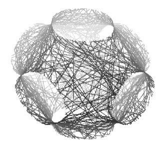
Figure 1: A typical trajectory in the three-dimensional configuration space ($\theta_{1}$, $\theta_{2}$, $\theta_{3})$ of the system (8), (9)

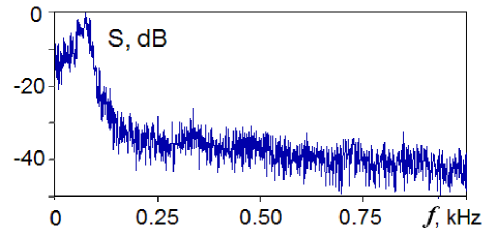
Figure 2: The power spectrum calculated for the variable $\cos\theta_{1}$ of the system (8), (9) for the motion with kinetic energy $W$=0.3

Taking into account the imposed mechanical constraint, there are four Lyapunov exponents characterizing perturbations near the reference phase trajectory: one positive, one negative and two zero ones. One exponent vanishes due to the autonomous nature of the system; it is responsible for a perturbation directed along the phase trajectory. The other is associated with a perturbation of the energy shift.

Since there is no characteristic time scale in the system, the Lyapunov exponents corresponding to the exponential growth and decrease of perturbations per unit time must be proportional to the velocity, i.e. $\lambda=\pm\kappa\sqrt{W}$, where the coefficient is determined by the average curvature of the metric. Empirically, for the system under consideration the calculations yield $\kappa=0.70$ 26 ; 27 .

.1.2 The triple linkage

Dynamics corresponding to the geodesic flow on the Schwartz surface takes place in the Thurston–Weeks–MacKay–Hunt triple hinge mechanism 24 ; 25 shown schematically in Fig. 3

The Cartesian coordinates of the hinges P_1,2,3 attached to the disks are expressed through the angles $\theta_{1}$, $\theta_{2}$, $\theta_{3}$, counted from the rays connecting the disk centers with the origin as follows:

$$\begin{array}[]{l}x_{1}+iy_{1}=1-re^{i\theta_{1}},\\ x_{2}+iy_{2}=-e^{2\pi i/3}(1-re^{i\theta_{2}}),\\ x_{3}+i\,y_{3}=-e^{-2\pi i/3}(1-re^{i\theta_{3}}).\\ \end{array}$$ (10)

The mechanical constraint provided by the rods and hinges implies that the radius of the circumscribed circle of the triangle P₁P₂P₃ must be $R$. By the known formula, $R=abc/4S$, where $a$, $b$, $c$ are sides of the triangle, and $S$ is its area. With given coordinates of three vertices ($x_{i}$, $y_{i})$, we evaluate the sides, and the area is expressed in terms of the vector product of vectors ${\rm{\bf b}}=P_{1}P_{2}$ and ${\rm{\bf c}}=P_{1}P_{3}$, $S=\textstyle{1\over 2}\left|{{\rm{\bf b}}\times{\rm{\bf c}}}\right|$. Thus, we have $(abc)^{2}-4R^{2}({\rm{\bf b}}\times{\rm{\bf c}})=0$, or

$$\begin{array}[]{c}[(x_{1}-x_{2})^{2}+(y_{1}-y_{2})^{2}]\cdot[(x_{2}-x_{3})^{2}+(y_{2}-y_{3})^{2}]\cdot[(x_{3}-x_{1})^{2}+(y_{3}-y_{1})^{2}]/4R^{2}\\ -(x_{2}y_{3}+x_{3}y_{1}+x_{1}y_{2}-x_{3}y_{2}-x_{1}y_{3}-x_{2}y_{1})^{2}=0.\\ \end{array}$$ (11)

Substituting the expressions from (10), we obtain the constraint equation in the form $F(\theta_{1},\theta_{2},\theta_{3})=0$.

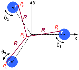
Figure 3: The triple linkage of Thurston–Weeks–MacKay–Hunt 24 ; 25 is made of three disks placed in a common plane, with centers at the vertices of an equilateral triangle, each of which is capable of rotating about its axis. On each disk at the edge a hinge is attached (P_1,2,3), and three identical rods are connected to these hinges, the opposite ends of which are joined together by another movable hinge (P₀)

Assuming $r<<1$ and expanding (11) in Taylor series up to terms of the first order in the small parameter, we obtain

$$27(R^{2}-1)-18r(2R^{2}-3)(\cos\theta_{1}+\cos\theta_{2}+\cos\theta_{3})=0.$$ (12)

With $R=1$ we arrive at the constraint equation, which is exactly the same as used in the context of the geodesic flow on the Schwarz surface (3). Under assumption that the only massive elements are the disks, with unit moment of inertia, the equations of motion are reduced exactly to the form (8).

.2 Self-oscillating systems with mechanical hinge connections

Suppose that additional torques $M_{1,2,3}$ are applied to the disks of the triple linkage system, then, in the assumptions we used, the equations are 26 ; 27

$$\ddot{\theta}_{1}=M_{1}-\Lambda\sin\theta_{1},\,\,\ddot{\theta}_{2}=M_{2}-\Lambda\sin\theta_{2},\,\,\ddot{\theta}_{3}=M_{3}-\Lambda\sin\theta_{3},$$ (13)

where

$$\Lambda=-\frac{\sum\nolimits_{j=1}^{3}{\left({\dot{\theta}_{j}^{2}\cos\theta_{j}+M_{j}\sin\theta_{j}}\right)}}{\sum\nolimits_{j=1}^{3}{\sin^{2}\theta_{j}}}.$$ (14)

Setting the torques as functions of the angular velocities, one can obtain various variants of self-oscillating systems demonstrating dynamics of the Anosov geodesic flow on their attracting sets.

.2.1 System with invariant energy surface

Consider first the case simplest for analysis as proposed qualitatively in 25 . Namely, we set

$$M_{i}=\left(\mu-\nu\sum\nolimits_{j=1}^{3}{\dot{\theta}_{j}^{2}}\right)\dot{\theta}_{i},\,\,i=1,2,3,$$ (15)

where $\mu$, $\nu$ are constants. In practice, to obtain such a function, the mechanism should be supplemented with a controlling device and actuators, which apply the torques $M_{1,2,3}$ to the axles of the disks depending on the value of the detected instant kinetic energy.

Equations (8) in this case read

$$\begin{array}[]{l}\ddot{\theta}_{i}=\left(\mu-\nu\sum\nolimits_{j=1}^{3}{\dot{\theta}_{j}^{2}}\right)\left({\dot{\theta}_{i}-\frac{\sum\nolimits_{j=1}^{3}{\dot{\theta}_{j}\sin\theta_{j}\sin\theta_{i}}}{\sum\nolimits_{j=1}^{3}{\sin^{2}\theta_{j}}}}\right)-\frac{\sum\nolimits_{j=1}^{3}{\dot{\theta}_{j}^{2}\cos\theta_{j}\sin\theta_{i}}}{\sum\nolimits_{j=1}^{3}{\sin^{2}\theta_{j}}},\\ i=1,2,3.\\ \end{array}$$ (16)

From this it is easy to derive an equation describing evolution of the kinetic energy $W=\textstyle{1\over 2}(\dot{\theta}_{1}^{2}+\dot{\theta}_{2}^{2}+\dot{\theta}_{3}^{2})$, namely,

$$\dot{W}=2(\mu-2\nu W)W.$$ (17)

Figure 4 shows the angular velocities of the disks and the energy versus time, in the course of the transient process of arising chaotic self-oscillations when starting with small initial velocity from a point in the configuration space admissible by the mechanical constraint. As a result, the self-oscillatory regime develops corresponding to a constant value of the kinetic energy, accompanied by irregular oscillations of the angular velocities evidently of chaotic nature (no repetitions of the waveforms are visible).

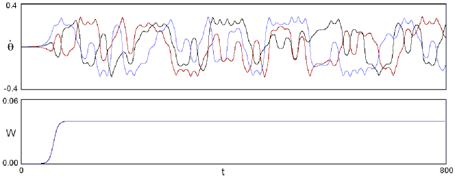
Figure 4: Evolution of the angular velocities $\dot{\theta}_{1},\,\,\dot{\theta}_{2},\,\,\dot{\theta}_{3}$ and energy $W$ in time in the course of transient process towards chaotic self-oscillations at $\mu$=0.12, $\nu$=1.5.

Formally, the phase space is six-dimensional, and there are six Lyapunov exponents characterizing behavior of perturbed phase trajectories near the reference orbit. Excluding two nonphysical zero exponents, which violate the constraint equation, we have four exponents in the rest. Since the motion on the attractor takes place on the energy surface, the exponents for perturbations without departure from this surface will be equal to those in the conservative system at the same energy: $\kappa\sqrt{W}$, 0, and $-\kappa\sqrt{W}$, $\kappa=0.70$ 26 ; 27 . The exponent corresponding to perturbation of the energy is evaluated easily as the Lyapunov exponent of the attracting fixed point $W=\mu$/2$\nu$ in Eq. (17); it is equal to $-2\mu$.

The observed attractor is undoubtedly hyperbolic since the dynamics takes place along geodesic lines of the metric of negative curvature on the energy surface, which is itself an attractive set. It is interesting, however, to try application of the criterion of angles in this case to test the methodology, which further will be exploited in situations where the presence or absence of hyperbolicity is not trivial.

The procedure begins with calculation of a reference orbit ${\rm{\bf x}}(t)$ on the attractor, for which numerical integration of the equations, briefly written in the form ${\rm{\bf\dot{x}}}={\rm{\bf F}}({\rm{\bf x}},t)$, is performed over a sufficiently long time interval. Being interested in the one-dimensional subspace associated with the largest Lyapunov exponent, we integrate the linearized equation for the perturbation vector along the reference trajectory: ${\rm{\bf\dot{\tilde{x}}}}={\rm{\bf{F}^{\prime}}}({\rm{\bf x}}(t),t){\rm{\bf\tilde{x}}}$. Normalizing the vectors ${\rm{\bf\tilde{x}}}$ at each step $n$, we obtain a set of unit vectors $\,\{{\rm{\bf x}}_{n}\}$. Next, we integrate a conjugate linear equation ${\rm{\bf\dot{u}}}=-[{\rm{\bf{F}^{\prime}}}({\rm{\bf x}}(t),t)]^{T}{\rm{\bf u}}$, where T denotes transpose, in inverse time along the same reference trajectory 41 . Then, we obtain a set of vectors $\,\{{\rm{\bf u}}_{n}\}$ normalized to unity that determine the orthogonal complement to the sum of the stable and neutral subspaces of the perturbation vectors at the reference trajectory. Now, to evaluate an angle $\phi$ between the subspaces at each $n$-th step, we calculate the angle $\beta_{n}\in$[0,$\pi$/2] between the vectors ${\rm{\bf\tilde{x}}}_{n}$, ${\rm{\bf u}}_{n}$, and set $\phi_{n}=\pi\mathord{\left/{\vphantom{\pi 2}}\right.\kern-1.2pt}2-\beta_{n}$.

Figure 5 shows histograms of the distributions of angles between stable and unstable subspaces numerically obtained for the system (16) with $\nu$=1.5 at $\mu$=0.12 and 0.75. As seen, the distributions are clearly distant from zero angles; so, the test confirms the hyperbolicity of the attractors.

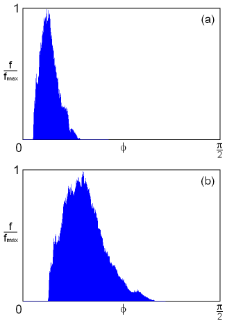
Figure 5: Verification of the hyperbolicity criterion for angles in a system (16) with invariant energy surface for $\mu$=0.12 and $\mu$=0.75 at $\nu$=1.5.

.2.2 System of three self-rotators with hinge constraint

Now let us turn to a system, where a torque applied to each disk depends only on the angular velocity of that disk. Namely, we set

$$M_{i}=(\mu-\nu\dot{\theta}_{1}^{2})\dot{\theta}_{i},\,\,i=1,2,3.$$ (18)

To provide such torques in a real device, one can use a pair of friction clutches attached to each disk, which transmit oppositely directed rotations, selecting properly the functional dependence of the friction coefficient on the velocity. In this case, each of the three disks is a self-rotator that means a subsystem, which, being singled out, manifests evolution in time with approach to a steady rotation with constant angular velocity $\dot{\theta}=\pm\sqrt{\mu\nu^{-1}}$ in one or other direction (depending on initial conditions).

Equations (3) in this case will be rewritten in the form

$$\ddot{\theta}_{i}=(\mu-\nu\dot{\theta}^{2})\left({\dot{\theta}_{i}-\frac{\sum\nolimits_{j=1}^{3}{\dot{\theta}_{j}\sin\theta_{j}}}{\sum\nolimits_{j=1}^{3}{\sin^{2}\theta_{j}}}\sin\theta_{i}}\right)-\frac{\sum\nolimits_{j=1}^{3}{\dot{\theta}_{j}^{2}\cos\theta_{j}}}{\sum\nolimits_{j=1}^{3}{\sin^{2}\theta_{j}}}\sin\theta_{i},\,\,i=1,2,3.$$ (19)

Figure 6 shows the angular velocities of the disks and the energy $W=\textstyle{1\over 2}(\dot{\theta}_{1}^{2}+\dot{\theta}_{2}^{2}+\dot{\theta}_{3}^{2})$ versus time in the transient process towards chaotic self-oscillations at $\mu$=0.06, $\nu$=1.5 starting with small initial velocity from a point in the configuration space admissible by the mechanical constraint. As a result of the transient process, a chaotic self-oscillatory regime arises, in which the kinetic energy fluctuates irregularly about a certain mean value. Figure 7 shows how the mean kinetic energy and its standard deviation depend on the supercriticality $\mu$.

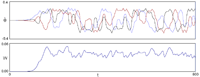
Figure 6: Angular velocities $\dot{\theta}_{1},\,\,\dot{\theta}_{2},\,\,\dot{\theta}_{3}$ and energy $W$ versus time in the transient process towards chaotic self-oscillations in a system of three self-rotators with mechanical constraint (19) at $\mu$=0.06, $\nu$=1.5.

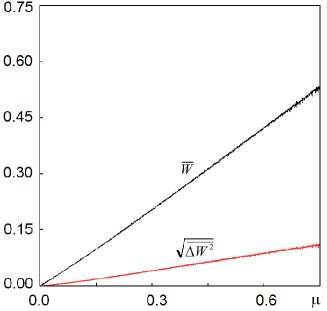
Figure 7: The mean kinetic energy of self-oscillations and the standard deviation of energy for the system of three self-rotators with mechanical constraint (19) with for $\nu=1.5$ versus the criticality parameter $\mu$

Concerning a number of significant Lyapunov exponents, the same reasoning is valid as for the previous model. Figure 9 shows a plot of the four Lyapunov exponents calculated by the Benettin algorithm 33 ; 34 ; 35 depending on the parameter $\mu$.

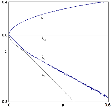
Figure 8: Lyapunov exponents of the dissipative system of three self-rotators with mechanical constraint depending on the parameter $\mu$ for $\nu$=1.5. Two nonphysical exponents violating the condition of mechanical constraint are excluded

Figure 9 shows histograms for distributions of the angles between stable and unstable subspaces obtained numerically for the system (16) with $\nu$ = 1.5 at $\mu$ = 0.06 and 0.39. As seen, the distributions are clearly distant from zero, the hyperbolicity of the attractors is confirmed.

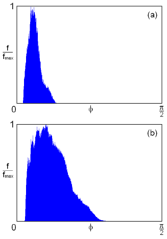
Figure 9: Verification of the hyperbolicity criterion for angles in the system of self-rotators with mechanical constraint for $\mu$=0.06 and $\mu$=0.39 at $\nu$=1.5

.3 System of three self-rotators with potential interaction

From systems with mechanical hinge constraints we turn now to situation when interaction of the rotators constituting the system is provided by a potential function depending on the angular variables in such way that the minimum takes place on the Schwartz surface: $U(\theta_{1},\theta_{2},\theta_{3})=\textstyle{1\over 2}(\cos\theta_{1}+\cos\theta_{2}+\cos\theta_{3})^{2}$. Instead of equations (13) we write now

$$\ddot{\theta}_{i}=-\partial U/\partial\theta_{i}+M_{i}=(\cos\theta_{1}+\cos\theta_{2}+\cos\theta_{3})\sin\theta_{1}+M_{i},\,\,i=1,2,3,$$ (20)

where $M_{1,2,3}$ are torques applied to the rotators. Assigning them according to (15) we get

$$\ddot{\theta}_{i}=(\mu-\nu\dot{\theta}_{i}^{2})\dot{\theta}_{i}-(\cos\theta_{1}+\cos\theta_{2}+\cos\theta_{3})\sin\theta_{i},\,\,i=1,2,3.$$ (21)

Figure 10 shows the dependencies of the generalized velocities of rotators and of the kinetic energy on time in the transient process in the system (21). As a result of the transient process, a chaotic self-oscillatory regime arises, where the kinetic energy fluctuates irregularly about a certain mean value.

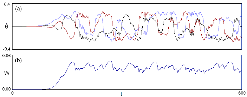
Figure 10: Plots for the angular velocities $\dot{\theta}_{1},\,\,\dot{\theta}_{2},\,\,\dot{\theta}_{3}$ and kinetic energy $W=\textstyle{1\over 2}(\dot{\theta}_{1}^{2}+\dot{\theta}_{2}^{2}+\dot{\theta}_{3}^{2})$ versus time in the transient process towards chaotic self-oscillations in the system (21) at $\mu$=0.06, $\nu$=1.5 (b)

Figure 11 illustrates behavior of the trajectories in the configuration space of the system (21). At small values of the parameter $\mu$, which corresponds to a small average energy in the sustained regime, the trajectories are located near the two-dimensional surface determined by the equation $\cos\theta_{1}+\cos\theta_{2}+\cos\theta_{3}=0$ corresponding to the mechanical constraint assumed in the previous sections. This gives foundation to expect that in this situation the hyperbolic dynamics are still preserved. However, already here one can observe that the trajectory is ”fluffed” in a direction transversal to the surface, which reflects the presence of fluctuations in the potential energy in the course of the motion. This effect, insignificant at small $\mu$, becomes more pronounced with increase of $\mu$, which can be seen in the diagram (b). One can expect, and this is confirmed by numerical calculations, that the nature of the attractor can change due to this effect, in particular, the dynamics may become non-hyperbolic.

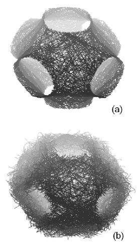
Figure 11: Trajectory on the attractor of the system (21) for $\mu$ = 0.06 (a) and $\mu$ = 0.75 (b) in the three-dimensional configuration space at $\nu$ = 1.5

Figure 12 shows the mean kinetic energy of self-oscillations and the root-mean-square deviation of energy versus parameter $\mu$ for the system of three self-rotators with potential interaction (21). In the left part of the plot the dependences look similar to those shown in Fig. 8, which indicates preservation of the same type of hyperbolic dynamics. However, with increase in the parameter, approximately at $\mu\approx$0.54, one can see a change in the nature of the dynamics. As calculations show, instead of chaos in the region, a regular regime occurs. It corresponds to a limit cycle in the phase space.

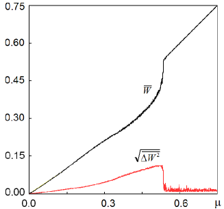
Figure 12: Plots of the mean kinetic energy of self-oscillations and the root-mean-square deviation of energy for a system of three rotators with potential interaction (21) for $\nu$ = 1.5

Figure 13 shows the Lyapunov exponents calculated using the Benettin algorithm 33 ; 34 ; 35 versus the parameter for the model (21). For this system, all six exponents should be taken into account in the analysis as there is no reason to exclude any of them from the consideration. The presence of a zero exponent is due to the autonomous nature of the system, and it is associated with perturbations of a shift along the reference trajectory.

In the region of small $\mu$ we have one positive, one zero, and the other negative Lyapunov exponents. Dependence of the exponents on the parameter is smooth here, without irregularities, which suggests that the hyperbolic chaos persists, as in the original model considered in Section 2. The senior Lyapunov exponent remains positive, and the dynamics is chaotic up to $\mu\approx$0.54. When approaching this point, brokenness arises and progresses in the graph of the senior exponent that apparently indicates destruction of the hyperbolicity, though no visible drops to zero with formation of regularity windows are distinguished. Then, the chaos disappears sharply, and the system manifests transition to the regular mode, where the senior exponent is zero, and the others are negative that corresponds to the limit cycle.

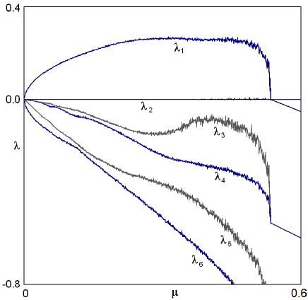
Figure 13: Lyapunov exponents of the system of three self-rotators with potential interaction (21), depending on the parameter $\mu$ for $\nu$=1.5

Figure 14 shows results of testing attractors of the model (21) using the criterion of angles. Here the numerically obtained histograms are plotted for the angles between stable and unstable subspaces of perturbation vectors for typical chaotic phase trajectories. At small values of $\mu$ the distributions are disposed at some finite distance from zero angles, i.e. the test confirms the hyperbolicity. This feature, however, is violated somewhere in the course of increase of $\mu$. Observe that the histogram (b) clearly demonstrates the presence of angles close to zero, which indicates occurrence of tangencies of stable and unstable manifolds, and, hence, signalizes about non-hyperbolic nature of the attractor. As this phenomenon was not observed in the models with hinge constraints, it is natural to assume that absence of hyperbolicity is linked with excursions of the phase trajectories relating to the attractor outside a narrow neighborhood of the surface of equal potential in the configuration space.

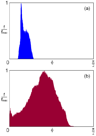
Figure 14: Verification of the criterion of angles for three rotators with potential interaction (21) at $\nu$=1.5 with $\mu$=0.06 (a) and $\mu$=0.39 (b). The histogram (a) shows a statistical distribution separated from zero that indicates the hyperbolic nature of the attractor. The diagram (b) shows a distribution with positive probability of angles close to zero indicating occurrences of touches of stable and unstable manifolds that means violation of the hyperbolicity.

.4 Electronic generator of rough chaos

To construct an electronic device on the principles discussed in the previous part of the article, elements analogous to rotators in mechanics are required. Namely, the state of such an element has to be characterized by a generalized coordinate defined modulo 2$\pi$ together with its derivative, the generalized velocity. An appropriate variable of such kind is a phase shift in the voltage controlled oscillator relative to a reference signal, like it is practiced in the phase-locked loops 32 ; 33 .

.4.1 Circuit diagram of the chaos generator and its functioning

The circuit shown in Fig. 3 is made up of three similar subsystems containing voltage-controlled generators, respectively, V1, V2, V3 (in the diagram they are marked with dashed rectangles). The oscillation phases of these generators are controlled by the voltages $U_{1}$, $U_{2}$, $U_{3}$ across the capacitors C1, C2, C3. Thus, the voltage outputs vary in time as $\sin(\omega t+\theta_{1,2,3})$, where the phases satisfy the equations

$$\frac{d\theta_{i}}{dt}=kU_{i},\,\,\,i=1,2,3.$$ (22)

Here $k$ is the steepness factor of frequency tuning of the voltage controlled generators; Specifically we take $k/2\pi=40$ kHz/V. The central frequency of the generators V1, V2, V3 is 20 kHz, which is provided by the bias voltage from the source V4. A reference signal with frequency $f=\omega/2\pi=$20 kHz and amplitude of 1 V is generated by the voltage source V5.

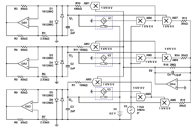
Figure 15: Circuit diagram of the chaos generator in the Multisim software package. Coefficient of frequency control for V1, V2, V3 is $k$/2$\pi$=40 kHz/V

We write now the Kirchhoff equations for the currents through the capacitors C1, C2, and C3, assuming that the output voltages of the analog multipliers AM1, AM2, AM3 are $W_{1,2,3}$. We have

$$C\frac{dU_{i}}{dt}+(R^{-1}-g)U_{i}+\alpha U_{i}+\beta U_{i}^{3}=\frac{W_{i}}{R},\,\,i=1,2,3,$$ (23)

where $C$ = C1 = C2 = C3 = 2 nF, $R$ = R10 = R11 = R12 = 100 kOhm, and $I(U)=\alpha U+\beta U^{3}$ is the characteristic of the nonlinear element composed of the diodes; its shape is shown in Fig.16. The equations take into account the negative conductivity $g=R_{2}/R_{1}R_{3}=R_{5}/R_{4}R_{6}=R_{8}/R_{7}R_{9}$ introduced by the elements on the operation amplifiers OA1, OA2, OA3. The voltages $W_{1,2,3}$ are obtained by multiplying the signals $\sin(\omega t+\theta_{1,2,3})\cos\omega t$ from AM4, AM5, AM6 by an output signal $W$ of the inverting summing-integrating element containing the operational amplifier OA4.

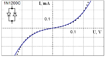
Figure 16: Volt-ampere characteristic of a nonlinear element composed of two parallel diodes 1N1200C. The differential resistance at low voltages is 2.602 kOhm. The points represent the data of Multisim simulating; the black curve is the approximation: $I(U)\approx\alpha U+\beta U^{3}$= 0.0039$U$+0.035$U^{3}$, where the current is expressed in amperes, and the voltage in volts

Input signals for the summing-integrating element are the output voltages of the multipliers AM7, AM8, AM9, which are expressed as $U_{1,2,3}\sin\omega t\sin(\omega t+\theta_{1,2,3})$, so, taking into account the leakage due to the resistor R16, for the voltage $W$ we can write

$$C_{0}\frac{dW}{dt}+\frac{W}{r}=-\frac{1}{R_{0}}\sum\limits_{i=1}^{3}{U_{i}\sin(\omega t+\theta_{i})\cos\omega t},$$ (24)

where C₀=C4=1.6 nF, $R_{0}$ =R13=R14=R15=20 kOhm, $r$=R16=2 MOhm.

Introducing normalized variables

$$\tau=\frac{t}{2\sqrt{RCR_{0}C_{0}}},\,\,\,u_{i}=2k\sqrt{RCR_{0}C_{0}}U_{i},\,\,\,w=2kR_{0}C_{0}W$$ (25)

and parameters

$$\Omega=2\sqrt{RCR_{0}C_{0}}\omega,\,\,\,\mu=2(gR-\alpha R-1)\sqrt{\frac{R_{0}C_{0}}{RC}},\,\,\nu=\frac{\beta}{2k^{2}C\sqrt{RCR_{0}C_{0}}},\,\,\,\gamma=\frac{2\sqrt{RCR_{0}C_{0}}}{r_{0}},$$ (26)

we obtain the equations

$$\begin{array}[]{l}\dot{\theta}_{i}=u_{i},\\ \dot{u}_{i}=\mu u_{i}-\nu u_{i}^{3}+2w\sin(\Omega\tau+\theta_{i})\cos\Omega\tau,\,\,\,\,i=1,\,\,2,\,\,3,\\ \dot{w}=-\gamma w-2\sum\limits_{i=1}^{3}{u_{i}\sin(\Omega\tau+\theta_{i})\cos\Omega\tau},\\ \end{array}$$ (27)

where the dot means the derivative over the dimensionless time $\tau$.

Taking into account that $\Omega\gg 1$ one can simplify the equations assuming that $u_{i}$ and $w$ vary slowly on the high-frequency period. Namely, we perform averaging in the right-hand parts setting

$$\overline{\sin(\Omega\tau+\theta_{i})\cos\Omega\tau}=\overline{\cos^{2}\Omega\tau\sin\theta_{i}+\sin\Omega\tau\cos\Omega\tau\cos\theta_{i}}=\textstyle{1\over 2}\sin\theta_{i}$$ (28)

and arrive at the equations

$$\begin{array}[]{l}\dot{\theta}_{i}=u_{i},\,\,\,\dot{u}_{i}=\mu u_{i}-\nu u_{i}^{3}+w\sin\theta_{i},\,\,i=1,\,\,2,\,\,3,\\ \dot{w}=-\gamma w-\sum\limits_{i=1}^{3}{u_{i}\sin\theta_{i}}.\\ \end{array}$$ (29)

Finally, supposing $\gamma\ll 1$ we can neglect the term $\gamma w$ in the last equation and to integrate it with substitution of $u_{1,2,3}$ from the first equation. Then we obtain $w\approx\cos\theta_{1}+\cos\theta_{2}+\cos\theta_{3}$, and the final result corresponds exactly to the equations (21).

.4.2 Circuit simulation

Figure 17 shows screenshots of the signals $U_{1,2,3}$ copied from the virtual oscilloscope screen when simulating the dynamics of the circuit in Multisim. Visually, the signals look chaotic, without any apparent repetition of forms. Figure 18 shows the spectrum of the signal $U_{1}$, obtained with the help of a virtual spectrum analyzer. Continuous spectrum, as it should be for a chaotic process, is characterized by slow decrease of the spectral density with frequency and is of rather good quality in the sense of lack of pronounced peaks and dips. Because of the symmetry of the circuit, all three time dependences for voltages $U_{1,2,3}$ are statistically equivalent, and their spectra as verified have the same form.

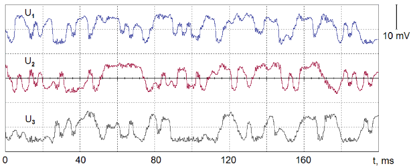
Figure 17: Voltages on capacitors C1, C2 and C3 obtained from the virtual oscilloscope screen when modeling the circuit in the Multisim environment. The scale along the vertical axis is indicated at the top in the right part of the figure

[!t]

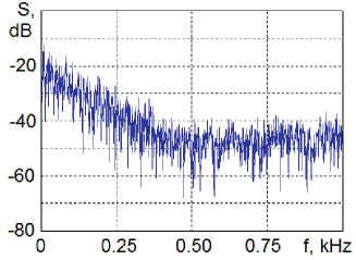
Figure 18: The power spectrum for the signal $U_{1}$ obtained as a snapshot from the virtual spectrum analyzer screen when modeling the dynamics of the circuit in the Multisim environment

To monitor the angular variables $\theta_{1,2,3}$ the circuit was supplemented by three special signal processing modules, in each of which the signal from the output of the voltage-controlled oscillators V1, V2, V3 was multiplied by the reference signals $\sin\omega t$ and $\cos\omega t$ (Fig. 19). After filtering with extraction of the low-frequency components, the obtained three pairs of signals ($x_{k}$, $y_{k})$, $k$=1,2,3, are fed to inputs of three oscilloscopes, and during the circuit operation, these signals are recorded into a file in computer for further processing with calculation of $\theta_{k}=\arg(x_{k}+iy_{k})$, $k$=1,2,3.

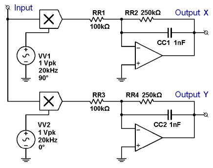
Figure 19: Signal processing module for constructing phase trajectories in the configuration space in circuit simulation. The circuit in Figure 15 was supplemented by three such modules, for which the input signals were time-varying voltages from the output of generators V1, V2, V3. It is essential that the alternating voltage sources VV1 and VV2 are phase shifted by 90 o relative to each other

.4.3 Dynamics of the chaos generator: numerics

In a framework of circuit simulation it is difficult to extract certain characteristics, for example, Lyapunov exponents, and it is not possible to verify the hyperbolic nature of chaos. Therefore, we turn to comparison of the results of numerical integration of the model equations (27), (29), and (21), for which the corresponding analysis can be performed in computations.

Using the nominal values of the circuit components in Fig. 16 and the formulas of the previous section, we find the parameters appearing in equations (27), (29) and (21):

$$\mu=0.07497,\,\,\nu=1.73156,\,\,\gamma=0.05,\,\,\,\Omega=20.1062.$$ (30)

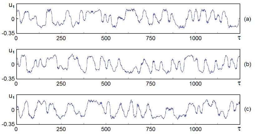
Figure 20: The time dependences of the variable $u_{1}$ obtained in the numerical solution of the equations for the models (27), (29) and (21), respectively, (a), (b) and (c)

Figure 20 shows plots for the dimensionless variable $u_{1}$ versus the dimensionless time obtained from the numerical integration of the equations (27) - panel (a), (29) - panel (b) and (21) - panel (c). Although there is no exact coincidence of the graphs on the diagrams (a), (b), (c) (because of the chaotic nature of the dynamics and its sensitivity to variations of the initial conditions), they are in reasonable agreement (note general view of the realizations and characteristic scales along the coordinate axes). This can be regarded as a confirmation of the validity of the approximations made in the course of sequential simplification of the model. This kind of correspondence can also be observed when comparing the graphs to the oscillograms in Fig. 17, obtained in the Multisim simulation.

Figure 21 shows power spectrum generated by the model (27), which is in reasonsble agreement with that obtained by the circuit simulation (Fig. 19), and with that of the system (8), (9) (Fig. 2).

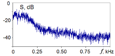
Figure 21: The power spectrum for the signal generated by the time dependence of the variable u1 in the model (27) with the parameters (30)

As one can verify, the dynamics of the electronic device proceeds in such a way that the trajectory in the space of coordinate variables ($\theta_{1}$,$\theta_{2}$,$\theta_{3})$ is located near the Schwarz surface. It is illustrated in Figure 22, where the trajectories obtained by numerical integration of the equations of the models (27), (21) and (21) are shown, respectively, in panels (a), (b), (c). They can be compared with Figure 1 for the original geodesic flow on the surface of negative curvature. It can be seen that the trajectories are close to the Schwartz surface, although they are not exactly located on it: they are slightly ”fluffy” in the transverse direction. This effect becomes more pronounced with increase of the parameter $\mu$.

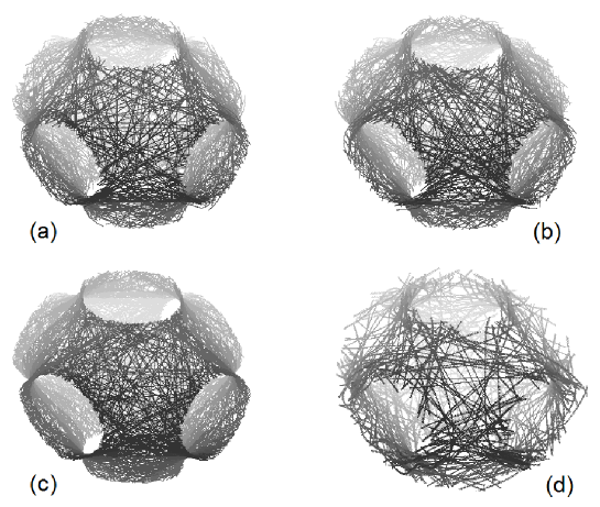
Figure 22: Trajectories in the three-dimensional space $(\theta_{1},\,\theta_{2},\,\theta_{3})$ for model systems described by equations (27) (a), (29) (b), and (21) (c), and for the electronic device simulated in Multisim corresponding to the scheme in Fig. 15 with the indicated nominal of the components (d)

The diagram (d) is obtained by processing data of circuit simulation in Multisim environment using the modification of the scheme described at the end of subsection 5.2. To construct the diagram by processing the recorded data, at each instant of time, three angular variables $\theta_{k}=\arg(x_{k}+iy_{k})$, $k$=1,2,3, were computed and a corresponding point was displayed on the graph. The diagram clearly demonstrates that the functioning of the device corresponds to dynamics on trajectories near the Schwarz surface, as well as in the models (27), (21), and (21).

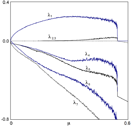
Figure 23: Lyapunov exponents of the system (27) depend on the parameter $\mu$ for the remaining parameters given in accordance with (20)

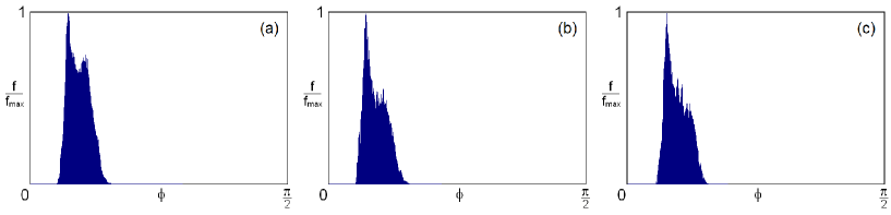
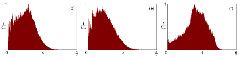
Figure 24: The histograms of the distribution of angles between stable and unstable subspaces obtained numerically: (a) in model (27), (b) in model (29) and (c) in model (21) for R_1,4,7=2.53 k$\Omega$, $\mu$=0.07497, when the distributions are distant from zero angles, and the attractor is hyperbolic. The bottom row represents histograms for the case of absence of hyperbolicity in model (27) (d), in model (29) (e) and in model (21) (f) for R_1,4,7=2.5 k$\Omega$, $\mu$=0.4544, when the distributions manifest presence of angles around zero.

Figure 23 shows a graph of seven Lyapunov exponents calculated for the model (27) using the Benettin algorithm 33 ; 34 ; 35 . In the entire range of the parameter $\mu$, we have one positive, two close to zero, and the other negative Lyapunov exponents. The dependence of the Lyapunov exponents on the parameter in this region is smooth, without peaks and dips, which allows us to assume that the hyperbolic nature of chaos retains.

In Fig. 24 histograms of the distributions of the angles obtained for the attractors of the systems (27), (21) and (21) are shown. The upper row corresponds to the parameters of the circuit in Fig. 15 (see (30)). For all three models the diagrams look similar, and the distributions are clearly separated from zero. Thus, the test confirms hyperbolicity of the attractor. For comparison, histograms obtained in the situation when hyperbolicity is violated are presented in the lower row, at sufficiently large $\mu$. In fact, they demonstrate a statistically significant presence of angles near zero, which indicates occurrence of tangencies of stable and unstable manifolds and nonhyperbolic nature of the attractor. Apparently, disappearance of the hyperbolicity occurs due to the deviating trajectories on the attractor from the Schwarz surface.

Conclusion

Hyperbolic chaos, which in dissipative systems corresponds to hyperbolic attractors, is characterized by roughness, or structural stability, as a mathematically rigorous attribute. Therefore, devices that generate such chaos must be preferred for any practical applications because of low sensitivity to variation of parameters, imperfections, disturbances, etc.

A reasonable approach to constructing systems with hyperbolic chaos is to start with a formal mathematical example, where such chaos takes place, and modify it by variations of functions and parameters in the respective equations. For small variations, the hyperbolic nature of the dynamics retains, as it is ensured by structural stability. However, as the detachment from the original system increases, violation of hyperbolicity becomes possible, and it should be monitored using quantitative criteria, one of which is analysis of the distribution of angles between stable and unstable manifolds of relevant trajectories.

In this paper we have considered several variants of systems with chaotic dynamics inspired by the problem of geodesic flow on a surface of negative curvature. Mechanical systems are based on the Thurston – Weeks – Hunt - MacKay hinge mechanism made up of three rotating disks. Their motions are either mechanically constrained with hinges and rods, or the constraint is replaced by potential interaction.

By analogy with the mechanical systems, a construction of electronic generator of rough chaos is proposed, electronic analog circuit is designed, corresponding equations are derived and computer study of the chaotic dynamics is carried out. The device was also modeled using the Multisim environment.

In contrast to the previously considered electronic circuits with hyperbolic attractors 40 ; 43 ; 44 ; 45 ; 46 ; 47 ; 48 , in this case hyperbolicity is characterized by an approximate uniformity in the expansion and compression of the phase volume elements in the course of evolution in continuous time. Due to this, the generator possesses rather good spectral properties providing a smooth distribution of the spectral power, without peaks and dips.

Although the specific scheme described in the article operates in a low-frequency range (kHz), it seems possible to build similar devices also in higher frequency bands.

References

- (1) S Smale, Bull. Amer. Math. Soc. (NS) 73, 747 (1967)
- (2) L Shilnikov International Journal of Bifurcation and Chaos in Applied Sciences and Engineering 7, 1353 (1997)
- (3) D V Anosov et al., Dynamical Systems IX: Dynamical Systems with Hyperbolic Behaviour, Encyclopaedia of Mathematical Sciences, vol. 9. (Springer. 1995)
- (4) A Katok and B Hasselblatt, Introduction to the Modern Theory of Dynamical Systems (Cambridge University Press, 1996)
- (5) Ya G Sinai, Selected Translations, Selecta Math. Soviet. 1(1), 100 (1981)
- (6) A A Andronov and L S Pontryagin, Dokl. Akad. Nauk. SSSR 14(5), 247 (1937)
- (7) A A Andronov, A A Vitt, SĖ Khaĭkin, Theory of oscillators (Pergamon, 1966).
- (8) M I Rabinovich and D I Trubetskov, Oscillations and waves: in linear and nonlinear systems (Springer Science & Business Media, 2012)
- (9) A P Kuznetsov, S P Kuznetsov, N M Ryskin, Nonlinear oscillations (Fizmatlit, Moscow, 2002) (Russian)
- (10) S Banerjee, J A Yorke and C Grebogi, Physical Review Letters 80, 3049 (1998)
- (11) Z Elhadj and J C Sprott, Robust Chaos and Its Applications (World Scientific: Singapore, 2011)
- (12) A S Dmitriev et al., Generation of chaos (Moscow, Technosfera, 2012) (Russian).
- (13) D V Anosov, Mathematical Events of the Twentieth Century, ed. A A Bolibruch, Yu S Osipov, and Ya G Sinai. (Springer-Verlag Berlin Heidelberg and PHASIS Moscow 2006), pp. 1-18.
- (14) Ya B Pesin, Lectures on partial hyperbolicity and stable ergodicity. Zurich lectures in advanced mathematics (European Mathematical Society, 2004)
- (15) C Bonatti, L J Diaz, and M Viana, Dynamics beyond Uniform Hyperbolicity. A Global Geometric and Probabilistic Perspective (Berlin, Heidelberg, New-York: Springer, 2005)
- (16) S P Kuznetsov, Phys. Uspekhi 54, 119 (2011)
- (17) S P Kuznetsov, Hyperbolic Chaos: A Physicist’s View (Berlin: Springer, 2012)
- (18) Y-C Lai et al., Nonlinearity 6, 779 (1993)
- (19) V S Anishchenko et al, Physics Letters A 270, 301 (2000)
- (20) F Ginelli et al., Physical Review Letters 99, 130601 (2007)
- (21) S P Kuznetsov, Physical Review Letters 95, 144101 (2005)
- (22) S P Kuznetsov and E P Seleznev, JETP 102, 355 (2006)
- (23) P V Kuptsov, Physical Review E 85, 015203 (2012)
- (24) S P Kuznetsov and V P Kruglov, Regular and Chaotic Dynamics 21, 160 (2016)
- (25) S P Kuznetsov and V I Ponomarenko, Technical Physics Letters 34, 771 (2008)
- (26) S P Kuznetsov, Regular and Chaotic Dynamics 20, 649 (2015)
- (27) S P Kuznetsov, Proceedings of Saratov University – New series. Series Physics 16(3), 131 (2016)
- (28) S P Kuznetsov, International Journal of Bifurcation and Chaos in Applied Sciences and Engineering 26, 1650232 (2016)
- (29) D V Anosov, Trudy Mat. Inst. Steklov 90, 3 (1967)
- (30) N L Balazs and A Voros Physics Reports 143(3), 109 (1986)
- (31) K Bums and V J Donnay, International Journal of Bifurcation and Chaos in Applied Sciences and Engineering 7, 1509 (1997)
- (32) S Sternberg, Curvature in mathematics and physics (Courier Corporation, 2012)
- (33) D J Struik, Lectures on classical differential geometry (Courier Dover Publications, 1988)
- (34) W H Meeks, J Pérez, A survey on classical minimal surface theory University Lecture Series, vol.60 (American Mathematical Society, 2012)
- (35) V I Arnol’d, Geometrical methods in the theory of ordinary differential equations (Springer Science & Business Media, 2012)
- (36) T J Hunt and R S MacKay, Nonlinearity 16, 1499 (2003)
- (37) S P Kuznetsov, Proceedings of Saratov University – New series. Series Physics 15(2), 5 (2015)
- (38) F R Gantmakher, Lectures in analytical mechanics (Moscow: Mir Publishers, 1970)
- (39) H Goldstein, Ch P Jr Poole, J L Safko, Classical Mechanics, 3d ed. (Boston, Mass.: Addison-Wesley, 2001)
- (40) W P Thurston and J R Weeks, Sci. Am. 251, 94 (1984)
- (41) G Benettin et al. Meccanica 15, 9 (1980)
- (42) H G Schuster and W Just, Deterministic chaos: an introduction (John Wiley & Sons, 2006)
- (43) S P Kuznetsov, Dynamical chaos (Fizmatlit, Moscow, 2001) (Russian)
- (44) V V Shakhgildyan and A A Lyakhovkin, Phase Locked Loops (Svyaz, Moscow, 1972) (Russian)
- (45) E Best Roland Phase-Locked Loops: Design, Simulation and Applications, 6th ed. (McGraw Hill, 2007)
- (46) S V Baranov, S P Kuznetsov and V I Ponomarenko, Izvestiya VUZ. Applied Nonlinear Dyanamics 18(1), 11 (2010)
- (47) S P Kuznetsov, Chaos: An Interdisciplinary Journal of Nonlinear Science 21, 043105 (2011)
- (48) D S Arzhanukhina, Vestnik Saratov State Technical University, No 3 (72) 20 (2013)
- (49) S P Kuznetsov, V I Ponomarenko, and E P Seleznev, Izvestiya VUZ. Applied Nonlinear Dyanamics 21(5), 17 (2013)
- (50) O B Isaeva et al., International Journal of Bifurcation and Chaos in Applied Sciences and Engineering 25, 1530033 (2015)