Transition path time distributions

Abstract

Biomolecular folding, at least in simple systems, can be described as a two state transition in a free energy landscape with two deep wells separated by a high barrier. Transition paths are the short part of the trajectories that cross the barrier. Average transition path times and, recently, their full probability distribution have been measured for several biomolecular systems, e.g. in the folding of nucleic acids or proteins. Motivated by these experiments, we have calculated the full transition path time distribution for a single stochastic particle crossing a parabolic barrier, focusing on the underdamped regime. Our analysis thus includes inertial terms, which were neglected in previous studies. These terms influence the short time scale dynamics of a stochastic system, and can be of experimental relevance in view of the short duration of transition paths. We derive the full transition path time distribution in the underdamped case and discuss the similarities and differences with the high friction (overdamped) limit.

I Introduction

Conformational changes of macromolecules between two different states are usually described by a transition in a double well potential landscape Hänggi, Talkner, and Borkovec (1990) (see Fig. 1). In this description one assumes that the complex collective behavior of the system can be mapped onto a single reaction coordinate. It is also typically assumed, as done in this work, that the reaction coordinate follows a stochastic memoryless Markovian dynamics (for a discussion of memory effects in molecular folding, see e.g. Walter et al. (2012); Sakaue et al. (2017); Satija, Das, and Makarov (2017); Vandebroek and Vanderzande (2017)).

If the barrier is high compared to the characteristic thermal energy $k_{B}T$, the molecule spends most of the time close to the minima, while the transition region around the barrier top is rarely visited. Transition paths are the part of the trajectories spent crossing the potential barrier connecting the two wells. Due to the very short duration of these trajectories, their experimental analysis has been a big challenge for a long time, but measurements of transition path times in nucleic acids and protein folding have been successfully performed in the past decade Chung, Louis, and Eaton (2009); Neupane et al. (2012); Truex et al. (2015); Neupane, Wang, and Woodside (2017). Transition paths have also attracted the attention of theorists and their properties were discussed in several papers Hummer (2004); Berezhkovskii and Szabo (2005); Dudko, Hummer, and Szabo (2006); Zhang, Jasnow, and Zuckerman (2007); Sega et al. (2007); Chaudhury and Makarov (2010); Orland (2011); Frederickx, In’t Veld, and Carlon (2014); Kim and Netz (2015); Makarov (2015); Daldrop, Kim, and Netz (2016); Berezhkovskii, Dagdug, and Bezrukov (2017).

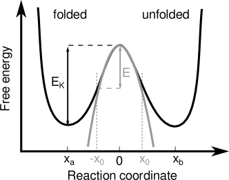
Figure 1: The complex motion of a system is often mapped onto the motion of a single reaction coordinate. Two-state systems are then imagined as the movement of this reaction coordinate in a one-dimensional free energy landscape, with two minima separated by an energy barrier $E$. To calculate the transition path time distribution, the top of the barrier is modelled as a parabolic barrier.

So far most of the theoretical studies focused on models of single particles crossing a one dimensional potential barrier in the overdamped regime in which friction forces dominate over inertia. In ordinary macromolecular dynamics, the high friction (overdamped) regime applies at typical experimentally sampled timescales. However, in view of the very short duration of transition paths, it is interesting to explore the underdamped regime in which inertial effects are taken into account. The aim of this paper is to discuss this regime.

We present analytical calculations of the distribution of transition path times (TPT’s) based on the Langevin equation with Gaussian white noise for a particle of mass $m$, and friction coefficient $\gamma$, which crosses a parabolic barrier $V(x)=-Kx^{2}/2$. In particular, we emphasize the differences with the TPT distribution in the overdamped limit, which has been already studied in the past Zhang, Jasnow, and Zuckerman (2007). The manuscript is organized as follows: Section II briefly recalls the setup for the analysis of overdamped particle dynamics and gives the underdamped Kramers’ time. Section III discusses the general setup of the problem and links the TPT probability distribution to an absorption probability. Section IV shows the details of the calculation of the TPT distribution for a parabolic barrier and discusses several regimes of the obtained expression. Section V discusses the behavior of the average TPT, while Section VI shows a comparison between the analytical results and numerical simulations.

II Review of underdamped dynamics

To analyze the underdamped dynamics of a particle of mass $m$, subject to an external force $F(x)$ and to a frictional force $-\gamma v$ we will make use of the Langevin equation Risken (1984)

$$m\ddot{x}=F(x)-\gamma\dot{x}+\eta(t),$$ (1)

where the dot indicates the time derivative and $\eta(t)$ is a Gaussian random force with properties

$$\begin{cases}\langle\eta(t)\rangle=0,\\ \langle\eta(t)\eta(t^{\prime})\rangle=2k_{\mathrm{B}}T\gamma\delta(t-t^{\prime}).\end{cases}$$ (2)

Here $\langle.\rangle$ denotes the average over different stochastic realizations.

Before discussing TPT it is convenient to recall some known results about Kramers’ time, which is the characteristic time for the particle to jump from one well to the other in a double well potential $V(x)$ as that shown in Fig. 1. This is obtained from the solution of Eq. (1), or of the associated Fokker-Planck equation. In the underdamped case the time for jumping from well $a$ to well $b$ is given by Hänggi, Talkner, and Borkovec (1990)

$$\tau_{a\to b}=2\pi\sqrt{\frac{K}{K_{a}}}\,\frac{2m\,e^{\displaystyle\beta E_{K}}}{\sqrt{\gamma^{2}+4Km}-\gamma},$$ (3)

where $E_{K}$ is the barrier height and $\beta=1/k_{B}T$. The Kramers’ time depends also on the curvature of the potential energy $V(x)$ at the bottom ($K_{a}$) and at the top ($K$) of the barrier, obtained from the expansions $V(x)\approx K_{a}(x-x_{a})^{2}/2$ and $V(x)\approx-Kx^{2}/2$. The overdamped regime can be obtained by letting $m\to 0$ in (3), which yields

$$\lim_{m\to 0}\tau_{a\to b}=\frac{2\pi\gamma}{\sqrt{K_{a}K}}\,e^{\displaystyle\beta E_{K}}\equiv\tau^{(o)}_{a\to b}$$ (4)

Note that the underdamped dynamics is always slower than the overdamped dynamics as $\tau>\tau^{(o)}$, i.e. inertia has the effect of slowing down the dynamics Hänggi, Talkner, and Borkovec (1990). Characteristic of the Kramers’ time is the exponential dependence on the barrier height.

III Transition path times distributions

In this Section we present the general framework for the calculation of $p_{\text{TP}}(t)$, the probability distribution that a transition path has a duration $t$. To define such paths one needs to fix the values of the reaction coordinates at the two sides of the barrier, as illustrated in Fig. 1. There is some freedom in the choice of the original and final point of transition paths, and the TPT distribution might depend on it. For convenience we place the maximum at $x=0$ and we consider paths from $-x_{0}<0$ to $x_{0}>0$. Transition paths are trajectories connecting the initial to the final point without entering the regions $x<-x_{0}$ and $x>x_{0}$.

The key quantity is the propagator $\mathcal{P}(x,v,t|x_{0},v_{0},0)$, which is the probability that a particle with initial position and velocity $x_{0}$ and $v_{0}$ is at $x$ and has velocity $v$ at a later time $t>0$. The calculation of TPT distributions requires thus absorbing boundary conditions at $-x_{0}$ and $x_{0}$. Consider a path originating at a point $x^{\prime}<x_{0}$ and with velocity $v^{\prime}$; in the underdamped case an absorbing region at $x>x_{0}$ means that Burschka and Titulaer (1981); Risken (1984)

$$\mathcal{P}(x_{0},v,t|x^{\prime},v^{\prime},0)=0\qquad\text{for}\quad v<0$$ (5)

which corresponds to setting to zero the current of particles leaving the wall towards the domain. Note that this is more subtle than the overdamped case for which more simply $\mathcal{P}(x_{0},t|x^{\prime},0)=0$. The condition (5) is more complicated to implement mathematically. No exact solution exists even for the simplest case of free diffusion with an absorbing boundary in the underdamped limit, and a set of approximation schemes has been devised Burschka and Titulaer (1981). However, for sufficiently steep barriers we expect that the solution with free boundary condition is a good approximation to the absorbing boundary case Zhang, Jasnow, and Zuckerman (2007). The approximation will be checked by comparing analytical results with numerical simulations.

In this work we will consider the initial velocity to be thermalized. This can be accounted for by integrating $\mathcal{P}$ over all possible initial velocities. In addition, as a transition path with free boundaries is defined by the fact that the particle crosses the $x_{0}$ boundary with any velocity, its final velocity has to be integrated over. We thus define

$$\text{P}(x,t|-x_{0},0)\equiv\int\limits_{-\infty}^{\infty}\mathrm{d}v\int\limits_{-\infty}^{\infty}\mathrm{d}v_{0}\;p_{\text{eq}}(v_{0})\mathcal{P}(x,v,t|-x_{0},v_{0},0),$$ (6)

where

$$p_{\text{eq}}(v)=\sqrt{\frac{m}{2\pi k_{B}T}}\,\,\,e^{-\displaystyle\frac{mv^{2}}{2k_{B}T}}$$ (7)

is the Maxwell velocity distribution for a system in equilibrium at temperature $T$, as we have assumed that the particles spend sufficiently long times in a given well, so that their positions and velocities follow an equilibrium distribution.

To connect the probability of finding the particle at position $x$ at a time $t$ to the TPT distribution, we introduce the absorption function $Q_{\mathrm{A}}$ obtained by integrating the function $\text{P}(x,t|-x_{0},0)$ obtained from Eq. (6) in the domain $x>x_{0}$:

$$Q_{\mathrm{A}}(t)\equiv\int\limits_{x_{0}}^{\infty}\mathrm{d}x\;\text{P}(x,t|-x_{0},0),$$ (8)

which counts all trajectories, originating in $-x_{0}$, that have already crossed the boundary $x_{0}$ at time $t$. Obviously, all these trajectories have a transition path time smaller than $t$, and thus $Q_{\mathrm{A}}(t)$ is proportional to the probability that the TPT is smaller than $t$.

The difference $Q_{\mathrm{A}}(t+\Delta t)-Q_{\mathrm{A}}(t)$ is thus equal to the fraction of trajectories that cross the boundary $x_{0}$ in the interval $[t,t+\Delta t]$, hence the TPT distribution can be approximated as

$$p_{\text{TP}}(t)\approx C\frac{dQ_{\mathrm{A}}(t)}{dt},$$ (9)

where $C$ is a normalization constant. This expression is approximate as we are not imposing the appropriate absorbing boundary conditions. When using free boundary conditions the left-hand side of Eq. (9) counts also paths with multiple crossings at $-x_{0}$ and $x_{0}$, which, strictly speaking, are not transition paths. However, in the high barrier limit, these paths become exceedingly rare and $Q_{\mathrm{A}}$ is a good approximation to the absorbing boundaries case. Finally, the normalization constant can be obtained from

$$\int_{0}^{+\infty}p_{\text{TP}}(t)dt = C\left[Q_{\mathrm{A}}(+\infty)-Q_{\mathrm{A}}(0)\right]$$ (10)

$$= CQ_{\mathrm{A}}(+\infty)=1,$$

where we have used $Q_{\mathrm{A}}(0)=0$, from Eq. (8).

IV TPT distribution for parabolic barrier

We consider here a parabolic barrier centered in $x=0$, which corresponds to a repulsive linear force

$$F(x)=Kx.$$ (11)

For this system the Langevin equation (1) is linear and can thus be solved. Denoting the solution by $x(t)$, the full propagator can be written as

$$\mathcal{P}(x,v,t|x_{0},v_{0},0)=\langle\delta(x-x(t))\delta(v-\dot{x}(t))\rangle.$$ (12)

As we saw in the previous section, the quantity of interest in Eq.(6) is

$$\text{P}(x,t|x_{0},0)=\int\limits_{-\infty}^{\infty}\mathrm{d}v\,\mathrm{d}v_{0}\;p_{\text{eq}}(v_{0})\langle\delta(x-x(t))\delta(v-\dot{x}(t))\rangle$$ (13)

The integration over the velocity $v$ is trivial (see details in Appendix A) and we find

$$\text{P}(x,t|x_{0},0)$$

$$\;\;=\int\limits_{-\infty}^{\infty}\mathrm{d}v_{0}\;p_{\text{eq}}(v_{0})\frac{1}{\sqrt{2\pi\phi^{2}(t)}}e^{-\displaystyle\frac{(x-X_{v_{0}}(t))^{2}}{2\phi^{2}(t)}}.$$ (14)

Here $X_{v_{0}}(t)$ is the solution of the deterministic equation of motion for a particle originating in $x_{0}$ and with initial velocity $v_{0}$ (see (A6)). The variance $\phi^{2}(t)$, given in Eq. (A7), does not depend on the initial conditions $x_{0}$ and $v_{0}$. It vanishes at short times, while it diverges exponentially at large times.

The next step is the integration in the initial velocities. Since $v_{0}$ enters linearly in $X_{v_{0}}$ and $p_{\text{eq}}(v_{0})$ is Gaussian, Eq. (6) boils down to a Gaussian integral which can be easily performed (for details see Appendix A). The result is

$$\text{P}(x,t|x_{0},0)=\frac{1}{\sqrt{2\pi\sigma^{2}(t)}}\,{e^{-\displaystyle\frac{\left(x-X_{0}(t)\right)^{2}}{2\sigma^{2}(t)}}},$$ (15)

where $X_{0}(t)$ is the deterministic solution of the equation of motion for a particle with vanishing initial velocity $v_{0}=0$. The resulting distribution (15) is again Gaussian, but with $\sigma^{2}(t)=\phi^{2}(t)+\psi^{2}_{v}(t)$, i.e. the variance is larger than that of the distribution (IV). Here $\psi^{2}_{v}(t)$ indicates the contribution obtained from integrating over the initial velocities (see Eq. (A13)).

The final step is the calculation of $Q_{\mathrm{A}}$, for which we get (details in Appendix A)

$$Q_{\mathrm{A}}(t)=\frac{1}{2}\left(1-\text{Erf}(G(t))\right),$$ (16)

where the error function is defined as

$$\text{Erf}(x)\equiv\frac{2}{\sqrt{\pi}}\int\limits_{0}^{x}\mathrm{d}u\;e^{-u^{2}}$$ (17)

and

$$G(t)\equiv\frac{x_{0}-X_{0}(t)}{\sqrt{2\sigma^{2}(t)}}.$$ (18)

The full expressions for $X_{0}(t)$ and $\sigma(t)$ are given in the Appendix A, Eqs. (A10) and (A12). Using Eqs. (9), (10) and the calculation of the normalization constant given in (A18), we arrive at the following expression for the TPT distribution:

$$p_{\text{TP}}(t)=-\frac{2}{\sqrt{\pi}}\frac{G^{\prime}(t)e^{-G^{2}(t)}}{1-\text{Erf}(\sqrt{\beta E})}.$$ (19)

where $G^{\prime}\equiv dG/dt$ is the time derivative of $G(t)$, $\beta=1/k_{B}T$ and $E=Kx_{0}^{2}/2$ is the barrier height.

The solid line in Fig. 2 shows a plot of the TPT distribution for an underdamped particle as given by Eq. (19). This distribution vanishes at short times, with a leading singular behavior due to the divergence of $G(t)$ in the limit $t\to 0$. From Eqs. (A10) and (A12) one finds at short times

$$p_{\text{TP}}(t){\underset{t\to 0}{\sim}}e^{-G^{2}(t)}=\exp\left(-\frac{2\beta mx_{0}^{2}}{t^{2}}\right).$$ (20)

This result can be understood from the ballistic motion of particles starting from $-x_{0}$. At short times the effect of the parabolic potential can be neglected and particles follow a free motion $x(t)\approx-x_{0}+vt$. The variance is then given by:

$$\sigma^{2}(t)=\langle\left(x(t)+x_{0}\right)^{2}\rangle\approx\langle v^{2}\rangle t^{2}=\frac{k_{B}T}{m}\,t^{2},$$ (21)

where we have used the equipartition theorem $m\langle v^{2}\rangle=k_{B}T$. Plugging in this result in Eq. (18) and recalling that $X_{0}(t)\approx-x_{0}$ at short times (Eq. (A10)) we obtain:

$$G^{2}(t)=\frac{\left(x_{0}-X_{0}(t)\right)^{2}}{2\sigma^{2}(t)}\,{\underset{t\to 0}{\sim}}\,\,\frac{2x_{0}^{2}}{\sigma^{2}(t)}=\frac{2mx_{0}^{2}}{k_{B}T}\,t^{-2},$$ (22)

which explains the result of Eq. (20).

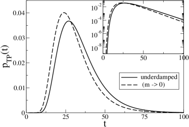
Figure 2: Transition path times distribution as obtained from Eq. (19) for an underdamped particle (solid line) and for the overdamped limit (dashed line) obtained by setting $m\to 0$. The characteristic behavior at short and long times is summarized in Table 1. The parameters used are, in dimensionless units, $x_{0}=-10$, $K=0.1$, $\gamma=1$, $m=1$ and $k_{\mathrm{B}}T=1$ corresponding to $\beta E=5$. Inset: the same data in semi-logarithmic scale to emphasize the exponential decay of the distribution at long times.

At long times $G(t)$ converges to a finite constant, since both the numerator and denominator in Eq. (18) diverge at the same rate. The calculation gives $G^{2}(t)\to\beta E$ (Eq. (A23)). However the derivative $G^{\prime}(t)$ vanishes exponentially at large $t$ (Eq. (A24)) as

$$G^{\prime}(t)\,{\underset{t\to\infty}{\sim}}\,e^{-\lambda_{+}t}$$ (23)

with

$$\lambda_{+}=\frac{-\gamma+\sqrt{\gamma^{2}+4Km}}{2m}$$ (24)

a characteristic rate of the process. The limiting behaviors of $G^{2}(t)$ and $G^{\prime}(t)$ are summarized in Table 1.

	rates	short times	long times
underd.	$\lambda_{\pm}\equiv\displaystyle{\frac{-\gamma\pm\sqrt{\Delta}}{2m}}$	$G^{2}(t)\sim\displaystyle\frac{2\beta mx_{0}^{2}}{t^{2}}$	$G^{\prime}(t)\sim-\sqrt{\beta E}\,\times$
	$\Delta=\gamma^{2}+4Km$		$\displaystyle{\frac{2\sqrt{\Delta}}{\gamma+\sqrt{\Delta}}}\lambda_{+}e^{-\lambda_{+}t}$
overd.	$\Omega\equiv\displaystyle{\frac{K}{\gamma}}$	$G^{2}(t)\sim\displaystyle\frac{\beta\gamma x_{0}^{2}}{t}$	$G^{\prime}(t)\sim-\sqrt{\beta E}\,\Omega e^{-\Omega t}$

Table 1: Summary of the asymptotic forms of $G(t)$ and $G^{\prime}(t)$ determining the behavior of the TPT distribution (19) at short and long times. Both the underdamped and overdamped regimes are given. (Note: short and long times correspond to the limits $\Omega t\ll 1$, $|\lambda_{\pm}t|\ll 1$ and $\Omega t\gg 1$, $|\lambda_{\pm}t|\gg 1$, respectively).

The overdamped regime

The overdamped limit is discussed in Appendix A.4 In this case the function $G(t)$ has a particularly simple expression:

$$G^{2}(t)=\beta E\,\frac{1+\exp(-\Omega t)}{1-\exp(-\Omega t)},$$ (25)

where $\Omega\equiv K/\gamma$ defines the characteristic rate of the overdamped system. This distribution was derived in Zhang, Jasnow, and Zuckerman (2007). The short time behavior is:

$$G^{2}(t)\approx\frac{2\beta E}{\Omega t}=\frac{\beta\gamma x_{0}^{2}}{t},$$ (26)

as expected from diffusive behavior of the particles we have at short times $2\sigma^{2}\approx 4Dt$, while the numerator $(x_{0}-X_{0}(t))^{2}\approx 4x_{0}^{2}$. Using the Einstein relation $D=k_{B}T/\gamma$ we recover Eq. (26). At long times $G^{2}(t)\to\beta E$ and

$$G^{\prime}(t)\approx-\sqrt{\beta E}\,\Omega e^{-\Omega t}$$ (27)

Comparing the overdamped and underdamped cases

Figure 2 shows a comparison of the underdamped TPT distribution (solid line) with the overdamped one, obtained by setting the mass term to zero (dashed line). Note that the values of the parameters chosen, given in the figure caption, correspond $\lambda_{+}=0.092$ while $\Omega=0.1$. Hence the differences between the two cases is expected to be rather small, as shown indeed in Fig. 2. The overdamped limit $m\to 0$ leads to a shift of the distribution to shorter timescales compared to the underdamped limit. Therefore inertia globally slows down the transition paths dynamics in analogy to the slowing down of Kramers’ times discussed above (Eqs. (3) and (4)). Note that at short time scales there is an opposite behavior with more faster crossings events in the underdamped regime (Eq. (20)) compared to the overdamped regime (Eq. (26) implies $p_{\text{TP}}(t)\sim\exp(\beta\gamma x_{0}^{2}/t)$). This behavior however involves a neglegible fraction of transition paths as shown in Fig. 2 (a second crossing between dashed and solind line takes place at short time scales, this is expected at times $1/|\lambda_{-}|\approx 0.92$).

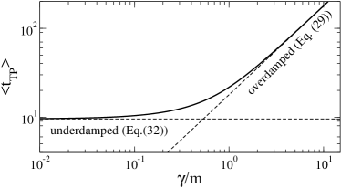
Figure 3: Solid line: average TPT plotted as a function of $\gamma/m$ in the larger barrier limit obtained from a numerical estimate of the integral in Eq. (28), with parameters $x_{0}=2$, $K=10$, $m=50$, $k_{\mathrm{B}}T=2$. Dashed lines: limiting values for $\langle t_{\text{TP}}\rangle$ in the over- and underdamped regime give by Eqs. (29) and (30), respectively.

V The average TPT

The average value of TPT is given by

$$\langle t_{\text{TP}}\rangle=\int_{0}^{+\infty}dt\,t\,p_{\text{TP}}(t)=\frac{\displaystyle\int_{\sqrt{\beta E}}^{+\infty}t(G)\,e^{-G^{2}}dG}{\displaystyle\int_{\sqrt{\beta E}}^{+\infty}e^{-G^{2}}dG}$$ (28)

where we have rewritten the integral using a change of variable $G^{\prime}dt=dG$. From the analysis of the previous section we have seen that $G(t)$ is a monotonic decreasing function of $t$ and $\sqrt{\beta E}\leq G\leq+\infty$.

We now present the results for the behaviour of the average TPT for large barrier. This asymptotic behavior is dominated by the behavior of $t(G)$ close to the lower bound $G\gtrsim\sqrt{\beta E}$, where both underdamped and overdamped TPT distributions decay exponentially (see Table 1). The details of the calculations can be found in the Appendix.

In the overdamped regime, Eq. (25) can be inverted easily to yield $t$ as a function of $G$, and we obtain asymptotically for large barrier $\beta E\gg 1$

$$\langle t_{\text{TP}}\rangle\approx\frac{\gamma}{K}\log(2e^{C}\beta E),$$ (29)

where $C\approx 0.577215$ is the Euler-Mascheroni constant. This result coincides with that previously obtained by A. Szabo Chung, Louis, and Eaton (2009).

In the underdamped regime, Eq. (18) cannot be inverted to yield $t$ as a function of $G$. However, using the asymptotic form of $G$, we show in the appendix that the large barrier limit of the average TPT is given by

$$\langle t_{\text{TP}}\rangle\approx\frac{1}{\lambda_{+}}\left(\log\beta E+A\right),$$ (30)

where $A$ is a constant independent of the barrier height given by

$$A=\log\left(\frac{4\sqrt{\Delta}}{\gamma+\sqrt{\Delta}}e^{C}\right),$$ (31)

where as above, $C$ is the Euler-Mascheroni constant. The other parameters are defined in the appendix and in Table 1. Note that this formula is quite general, as it yields back the overdamped case (29) in the limit of vanishing mass. In the limiting case of $\gamma\to 0$ Eqs. (30) and (31) become

$$\langle t_{\text{TP}}\rangle=\sqrt{\frac{m}{K}}\,\log\left(4e^{C}\beta E\right)$$ (32)

Figure 3 shows a plot of $\langle t_{\text{TP}}\rangle$ obtained by numerical integration of the probability distribution of TPT as a function of the ratio $\gamma/m$. At very high friction $\gamma^{2}\gg 4Km$ the calculation reproduces the overdamped limit (29). At low friction $\gamma^{2}\ll\Delta\approx 4Km$ (29) converges to a friction independent limit, shown by the dashed horizontal line in Fig. 3. Some words of caution are necessary when dealing with the low friction limit. It is well known Hänggi, Talkner, and Borkovec (1990) that the theory developed here is not valid when the friction becomes arbitrary small, but one still needs $\gamma\beta E\gg\sqrt{K/m}$. For friction below this limit the particles do not thermalize at the bottom of one well and the use of Eqs. (6) and (7) is not justified. As for the Kramers’ time one expects an increase in the average TPT at very low friction (known as Kramers’ turnover Hänggi, Talkner, and Borkovec (1990)).

VI Numerical Results

To assert the range of validity of the analytical calculations, numerical simulations were performed. This was done by numerically integrating the Langevin equation (1) using the algorithm developed by Vanden-Eijnden and CiccottiVanden-Eijnden and Ciccotti (2006).

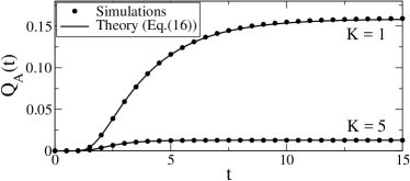
Figure 4: Comparison between analytical and numerical estimates of absorption probabilities $Q_{\mathrm{A}}$ for a thermalized set of particles started at $x=-x_{0}$. The parameters are $x_{0}=1$, $m=1$, $\gamma=1$ and $T=1$. Two values of $K$ have been simulated.

The absorption probability $Q_{\mathrm{A}}$

We run a first set of simulations using free boundary conditions and calculated the absorption probability $Q_{\mathrm{A}}(t)$. As the analytical expression (8) was also obtained with free boundary conditions, analytical and numerical results must coincide. The runs are used to test the accuracy of the integration scheme. To obtain $Q_{\mathrm{A}}(t)$ from simulations an ensemble of thermalized particles was put at the initial position $x=-x_{0}$ and subsequently evolved through time. At regular time intervals the number of particles in the region $x(t)>x_{0}$ was counted, which is, after normalizing by dividing through the total number of particles, a direct measure of $Q_{\mathrm{A}}$. The result of the simulation is shown on Fig. 4 for two different values of the barrier curvature $K=1$ and $K=5$. At long times the absorption probability saturates to a constant, which decreases as $K$ is increased since a smaller fraction of particles cross the barrier as this becomes steeper.

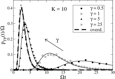
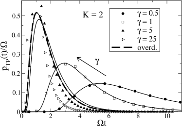
Figure 5: Solid lines: underdamped TPT distributions obtained from Eq. (19) for various $K$ and $\gamma$. Dashed lines: overdamped TPT distributions. Note that the solid line and dashed line coincide for the highest friction data. Symbols: TPT distributions from simulations. The other parameters are $x_{0}=1$ and $k_{B}T=1$. Deviations are observed between theory and experiments for $K=2$ and high friction (see discussion in the text).

The TPT distribution

We computed next the TPT distribution from simulations imposing absorbing boundary conditions in $x_{0}$. In order to obtain sufficient statistics a forward flux sampling scheme Allen, Warren, and ten Wolde (2005) was employed. In this scheme the transition path is created step by step rather than at once. The dynamics of the particles still starts at $-x_{0}$, but instead of waiting until one of them hits $x_{0}$, we evolve them until they hit $-x_{0}+\epsilon$ (where $\epsilon$ is a small, positive number), where we store the physical state of the particle. On the other hand, whenever a particle ventures into $x\leq-x_{0}$, we discard it and restart the simulation for that particle. This procedure is repeated until a representative ensemble at $-x_{0}+\epsilon$ is generated. In the next step, we evolve the particles from $-x_{0}+\epsilon$ to $-x_{0}+2\epsilon$, where we sample the initial conditions for this step from the ensemble generated by the particles that reached $-x_{0}+\epsilon$ in the previous step. Here again, the physical state is stored whenever $-x_{0}+2\epsilon$ is reached, or we discard and restart when $x\leq-x_{0}$. These steps are repeated until $x_{0}$ is reached.

Figure 5 shows plots of TPT distribution obtained for various values of the parameters and compares simulations (symbols) with the theory from Eq. (19) (solid lines). The dashed line is the overdamped distribution which overlaps with Eq. (19) for the highest value of the friction ($\gamma=25$). The data are plotted in rescaled time unit $\Omega t$, where $\Omega=K/\gamma$ is the characteristic rate of the overdamped case. The two plots correspond to two values of the barrier stiffness $K=2$ and $K=10$, while $x_{0}=1$ and $k_{B}T=1$. For each set we plot four different values of $\gamma$ (where the arrow indicates the direction of increasing $\gamma$).

For the steeper barrier ($K=10$) there is an excellent agreement between theory and simulations for all values of $\gamma$. In this case there is practically no difference between the free boundary conditions (theory) and the absorbing boundary conditions (simulations). This is in line with previous studies of the overdamped distributions Zhang, Jasnow, and Zuckerman (2007). Deviations are instead observed in the $K=2$ data, which are clearly visible at high friction, close to the overdamped limit. Here the analytical calculation overestimates the TPT, leading to a broader distribution compared to the simulations. This is because the theory with free boundary conditions wrongly counts as TP also those trajectories with multiple crossings at the boundaries and these trajectories lead to high TPT. At low friction and $K=2$, however, theory and simulation match again. This agreement can be understood as follows. As highlighted in the calculations of Section IV there are two contributions to the noise. Firstly, there is an intrinsic noise, contributing to the variance $\phi^{2}(t)$ in Eq. (IV). Secondly, the thermalization over different initial velocities leads to an additional contribution $\psi^{2}_{v}(t)$ to the variance, so that the total variance is $\sigma^{2}(t)=\phi^{2}(t)+\psi^{2}_{v}(t)$ (see Eq. (A13)), A simple analysis shows that $\phi^{2}(t)$ vanishes at low $\gamma$, whereas $\psi^{2}_{v}(t)$ converges to a non-vanishing constant. At small friction the trajectories are weakly influenced by thermal noise, particles will follow closely the deterministic trajectory, hence in the free boundary case multiple crossings of the boundary at $x_{0}$ will be rare. This is the reason of the agreement between theory and simulations. Note that the predominant contribution to the width of the TPT distribution comes in this limit from $\psi^{2}_{v}(t)$, i.e. the distribution of initial velocities.

VII Discussion

Conformational transitions molecular systems between two different states are governed by two time scales. The Kramers time corresponds to the typical time spent in a given conformation, while the transition path time characterizes the actual duration of the transition. Transition path times, which have been measured in protein and nucleic acids folding experiments during the past decade Chung, Louis, and Eaton (2009); Neupane et al. (2012); Truex et al. (2015); Neupane, Wang, and Woodside (2017), can be a few orders of magnitudes shorter than Kramers’ times.

In this paper we have analyzed the TPT distribution of a simple one dimensional stochastic particle undergoing Langevin dynamics and crossing a parabolic barrier. We focused in particular to the underdamped case, thus extending previous analysis Zhang, Jasnow, and Zuckerman (2007) in which inertial terms were neglected. As the barrier is parabolic, the associated Langevin equation is linear and hence exactly solvable. The inclusion of inertia makes the calculations more complex than in the overdamped limit, but an analytical form of the TPT distribution can still be obtained. This solution is not exact as it does not use the appropriate absorbing boundary conditions, but it approximates very well the numerical simulations for steep barriers.

In general inertia slows down the barrier crossing process. The main properties of the TPT distribution have been summarized in Table 1. The distribution has an essential singularity at short times, which is however of different nature in the overdamped and underdamped cases. At long times the distribution vanishes exponentially in both cases. Differently from the Kramers’ time, which is characterized by an exponential dependence on the barrier height $E$, the average TPT in the overdamped limit scales logarithmically $\langle t_{\text{TP}}\rangle\sim\log(\beta E)$, where $\beta$ is the inverse temperature. We have shown here that the logarithmic dependence also holds in the underdamped limit and have calculated the prefactor.

We conclude by remarking that, although in the analysis of the dynamics of molecular systems the overdamped limit is usually considered, owing to the short duration of TPT it is possible that inertial effects influence the barrier crossing dynamics. The availability of an analytical closed form of the TPT distribution in the underdamped case may indeed be useful for the analysis of future experiments.

Appendix A Details of the derivation of the TPT distribution

We give here all the details of the calculations, which were just briefly outlined in Section III.

A.1 The probability distribution

The solution of the second order linear differential equation

$$m\ddot{x}=Kx-\gamma\dot{x}+\eta(t).$$ (A1)

with initial conditions $x(0)=-x_{0}$ and $\dot{x}(0)=v_{0}$ is given by

$$x(t)=\frac{m}{\sqrt{\Delta}}\left[e^{\lambda_{+}t}(\lambda_{-}x_{0}+v_{0})\,-\,e^{\lambda_{-}t}(\lambda_{+}x_{0}+v_{0})\right]+\frac{1}{\sqrt{\Delta}}\int_{0}^{t}\mathrm{d}\tau\;\left(e^{\lambda_{+}(t-\tau)}\,-\,e^{\lambda_{-}(t-\tau)}\right)\eta(\tau),$$ (A2)

where the rate constants are given by:

$$\lambda_{\pm}=\frac{-\gamma\pm\sqrt{\Delta}}{2m}$$ (A3)

and

$$\Delta\equiv\gamma^{2}+4mK.$$ (A4)

Note that $\lambda_{+}>0$, $\lambda_{-}<0$ and $\lambda_{+}-\lambda_{-}=\sqrt{\Delta}/m$. In addition in the high friction limit $\gamma^{2}\gg 4mK$ one has

$$\lambda_{+}\approx\frac{K}{\gamma}\qquad\text{and}\qquad\lambda_{-}\approx-\frac{\gamma}{m}$$ (A5)

where in this limit $\lambda_{+}$ describes the deterministic dynamics of an overdamped particle “sliding down” in a parabolic potential: the equation of motion is $\gamma\dot{x}=Kx$ and the solution, with initial condition $x(0)=-x_{0}$ is $x(t)=-x_{0}e^{Kt/\gamma}$. The factor $1/|\lambda_{-}|$ is the timescale beyond which inertia effects are negligible.

Averaging (A2) over different noise realizations we obtain the solution of the deterministic equation of motion

$$X_{v_{0}}(t)\equiv\langle x(t)\rangle=\frac{m}{\sqrt{\Delta}}\left[e^{\lambda_{+}t}(\lambda_{-}x_{0}+v_{0})\,-\,e^{\lambda_{-}t}(\lambda_{+}x_{0}+v_{0})\right]$$ (A6)

where the subscript $v_{0}$ indicates the initial velocity (the solution obviously also depends on the initial position $-x_{0}$, however we omit to indicate this explicitly). Using Eqs. (2) we obtain for the variance:

$$\phi^{2}(t) \equiv \left\langle(x(t)-X_{v_{0}}(t))^{2}\right\rangle=\frac{1}{\Delta}\int_{0}^{t}d\tau d\tau^{\prime}\left(e^{\lambda_{+}(t-\tau)}\,-\,e^{\lambda_{-}(t-\tau)}\right)\left(e^{\lambda_{+}(t-\tau^{\prime})}\,-\,e^{\lambda_{-}(t-\tau^{\prime})}\right)\langle\eta(\tau)\eta(\tau^{\prime})\rangle=$$ (A7)

$$= \frac{2k_{\mathrm{B}}T\gamma}{\Delta}\int_{0}^{t}d\tau\left(e^{\lambda_{+}(t-\tau)}\,-\,e^{\lambda_{-}(t-\tau)}\right)^{2}=\frac{2k_{\mathrm{B}}T\gamma}{\Delta}\left[\frac{e^{2\lambda_{+}t}-1}{2\lambda_{+}}\,-\,2\frac{e^{(\lambda_{+}+\lambda_{-})t}-1}{\lambda_{+}+\lambda_{-}}\,+\,\frac{e^{2\lambda_{-}t}-1}{2\lambda_{-}}\right].$$

As $x(t)$ is a sum of gaussian stochastic variables (Eq. (A2)), is itself a gaussian stochastic variable and it is fully characterized by its average and variance. Therefore, we have

$$\mathcal{P}(x,v,t\,|\,-x_{0},v_{0},0)=\frac{1}{\sqrt{2\pi\phi^{2}}}\exp\left[-\frac{(x-X_{v_{0}}(t))^{2}}{2\phi^{2}}\right].$$ (A8)

To perform the integral over initial velocities (6) it is convenient to rewrite $X_{v_{0}}$ into two parts, separating the terms containing $v_{0}$

$$X_{v_{0}}(t)=X_{0}(t)+\frac{mv_{0}}{\sqrt{\Delta}}\left(e^{\lambda_{+}t}-e^{\lambda_{-}t}\right),$$ (A9)

where:

$$X_{0}(t)\equiv\frac{mx_{0}}{\sqrt{\Delta}}\left(\lambda_{-}e^{\lambda_{+}t}\,-\,\lambda_{+}e^{\lambda_{-}t}\right),$$ (A10)

describes the deterministic motion of the underdamped particle with initial conditions $x(0)=x_{0}$ and $\dot{x}(0)=0$.

The integral over $v_{0}$ in (6) is a shifted gaussian distribution and the result is:

$$\text{P}(x,t\,|\,-x_{0},0)=\frac{1}{\sqrt{2\pi\sigma^{2}}}\exp\left[-\frac{\left(x-X_{0}(t)\right)^{2}}{2\sigma^{2}}\right],$$ (A11)

where

$$\sigma^{2}(t)=\phi^{2}(t)+\frac{mk_{\mathrm{B}}T}{\Delta}\left(e^{\lambda_{+}t}-e^{\lambda_{-}t}\right)^{2}=\frac{2mk_{B}T}{\Delta}\left[-\frac{\lambda_{-}}{2\lambda_{+}}\left(e^{2\lambda_{+}t}-1\right)-\frac{\lambda_{+}}{2\lambda_{-}}\left(e^{2\lambda_{-}t}-1\right)+e^{(\lambda_{+}+\lambda_{-})t}-1\right]$$ (A12)

which shows that the averaging over initial velocities leads to an increase in the variance by a factor:

$$\psi_{v}^{2}(t)\equiv\frac{mk_{\mathrm{B}}T}{\Delta}\left(e^{\lambda_{+}t}-e^{\lambda_{-}t}\right)^{2}$$ (A13)

A.2 The transition path time distribution

The next step is the calculation of the absorption function

$$Q_{\mathrm{A}}(t)\equiv\int_{x_{0}}^{\infty}\mathrm{d}x\;\text{P}(x,t\,|\,-x_{0},0)=\int_{x_{0}}^{\infty}\mathrm{d}x\;\frac{1}{\sqrt{2\pi\sigma^{2}}}\exp\left[-\frac{\left(x-X_{0}(t)\right)^{2}}{2\sigma^{2}}\right].$$ (A14)

Using the following definition of the error function

$$\text{Erf}(t)\equiv\frac{2}{\sqrt{\pi}}\int_{0}^{t}\mathrm{d}u\;e^{-u^{2}},$$ (A15)

we can explicitly write the absorption rate as:

$$Q_{\mathrm{A}}(t)=\frac{1}{2}\Big{(}1-\text{Erf}\,(G(t))\Big{)},$$ (A16)

where

$$G(t)\equiv\frac{x_{0}-X_{0}(t)}{\sqrt{2\sigma^{2}(t)}}.$$ (A17)

To obtain the appropriate normalization we need to calculate the $t\to\infty$ behavior of $G(t)$. One finds $G^{2}(t)\to\beta E$ (see Eq. (A23)), where $\beta=1/k_{B}T$ is the inverse temperature and $E\equiv Kx_{0}^{2}/2$ the potential barrier that the particle needs to overcome. From the previous results we obtain:

$$\lim_{t\to\infty}Q_{\mathrm{A}}(t)=\frac{1}{2}\lim_{t\to\infty}\left(1-\text{Erf}\,(G(t))\right)=\frac{1}{2}\left(1-\text{Erf}\,(\sqrt{\beta E})\right)$$ (A18)

The TPT distribution is then given by the derivative of $Q_{\mathrm{A}}$ with respect to time:

$$p_{TP}(t)=\frac{1}{Q_{\mathrm{A}}(\infty)}\frac{\mathrm{d}Q_{\mathrm{A}}(t)}{\mathrm{d}t}=\frac{1}{2Q_{\mathrm{A}}(\infty)}\frac{\mathrm{d}}{\mathrm{d}t}\left(-\text{Erf}\left(G(t)\right)+1\right)=-\frac{2}{\sqrt{\pi}}\frac{G^{\prime}(t)e^{-G^{2}(t)}}{1-\text{Erf}(\sqrt{\beta E})}.$$ (A19)

where $G^{\prime}(t)\equiv dG/dt$.

A.3 Asymptotic behavior

At short times $|\lambda_{\pm}|t\ll 1$, we can expand the exponentials in the above expression for small values of the arguments. Expanding the exponential to lowest orders we find

$$\sigma^{2}(t)\approx\frac{2mk_{B}T}{\Delta}\,\left[-\lambda_{-}\lambda_{+}-\lambda_{+}\lambda_{-}+\frac{\left(\lambda_{+}+\lambda_{-}\right)^{2}}{2}\right]t^{2}=\frac{2mk_{B}T}{\Delta}\frac{\left(\lambda_{+}-\lambda_{-}\right)^{2}}{2}\,t^{2}=\frac{k_{B}T}{m}t^{2}$$ (A20)

which is the expected result from the equipartition theorem, as discussed in Section IV. At long times (recall that $\lambda_{-}<0$ and $\lambda_{+}+\lambda_{-}<0$) one has

$$\sigma^{2}(t)\approx-\frac{mk_{B}T\lambda_{-}}{\Delta\lambda_{+}}\,e^{2\lambda_{+}t}\left(1+{\cal O}\left(e^{-2\lambda_{+}t}\right)\right)$$ (A21)

and

$$\left(x_{0}-X_{0}(t)\right)^{2}\approx\left(x_{0}-\frac{mx_{0}}{\sqrt{\Delta}}\lambda_{-}e^{\lambda_{+}t}\right)^{2}\approx\frac{m^{2}x_{0}^{2}\lambda_{-}^{2}}{\Delta}e^{2\lambda_{+}t}\left(1-\frac{2\sqrt{\Delta}}{m\lambda_{-}}e^{-\lambda_{+}t}\right)$$ (A22)

Hence

$$G^{2}(t)\equiv\frac{\left(x_{0}-X_{0}(t)\right)^{2}}{2\sigma^{2}}\approx-\frac{m^{2}x_{0}^{2}\lambda_{-}^{2}}{2\Delta}\frac{\Delta\lambda_{+}}{mk_{B}T\lambda_{-}}\left(1-\frac{2\sqrt{\Delta}}{m\lambda_{-}}e^{-\lambda_{+}t}\right)=\beta E\left(1+\frac{4\sqrt{\Delta}}{\gamma+\sqrt{\Delta}}e^{-\lambda_{+}t}\right)$$ (A23)

where we have used $\lambda_{+}\lambda_{-}=-K/m$ and $E=Kx_{0}^{2}/2$ for the barrier height. From the previous equation we obtain the long time expansion of the derivative

$$G^{\prime}(t)\approx-\sqrt{\beta E}\frac{\sqrt{\Delta}}{\gamma+\sqrt{\Delta}}\lambda_{+}e^{-\lambda_{+}t}$$ (A24)

A.4 The overdamped regime

Having described the general underdamped case we illustrate now the solution of the overdamped case. For the initial condition $x(0)=-x_{0}$ we find:

$$x(t)=-x_{0}e^{\Omega t}+\frac{1}{\gamma}\int_{0}^{t}e^{\Omega(t-\tau)}\eta(\tau)$$ (A25)

where we have introduced the characteristic rate $\Omega\equiv K/\gamma$. In the overdamped case there is a single rate. We also note that $\lambda_{+}\to\Omega$ in the overdamped case at strong friction (see (A5)). The average of $x(t)$ corresponds to the deterministic trajectory of a particle sliding down from the potential barrier

$$X(t)\equiv\left\langle x(t)\right\rangle=-x_{0}e^{\Omega t}$$ (A26)

The variance is:

$$\sigma^{2}(t)\equiv\left\langle\left(x(t)-X(t)\right)^{2}\right\rangle=\frac{k_{B}T}{K}\,\left(e^{2\Omega t}-1\right)$$ (A27)

from which we get:

$$G^{2}(t)\equiv\frac{\left(x_{0}-X(t)\right)^{2}}{2\sigma^{2}(t)}=\frac{x_{0}^{2}\left(e^{\Omega t}+1\right)^{2}}{\frac{2k_{B}T}{K}\left(e^{2\Omega t}-1\right)}={\beta E}\,\frac{1+e^{-\Omega t}}{1-e^{-\Omega t}}$$ (A28)

One can get to the same results by using the expressions obtained in the overdamped case by formally taking the limit $m\to 0$. In this limit $\lambda_{-}t\to-\infty$ and $(\lambda_{+}+\lambda_{-})t\to-\infty$. From Eq. (A12) one gets:

$$\sigma^{2}\to\frac{2mk_{B}T}{\Delta}\left(-\frac{\lambda_{-}}{2\lambda_{+}}e^{2\lambda_{+}t}+\frac{\lambda_{-}}{2\lambda_{+}}+\frac{\lambda_{+}}{2\lambda_{-}}-1\right)=-\frac{mk_{B}T\lambda_{-}}{\Delta\lambda_{+}}\left[e^{2\lambda_{+}t}-\left(\frac{\lambda_{+}+\lambda_{-}}{\lambda_{-}}\right)^{2}\right]\to\frac{k_{B}T}{K}\left(e^{2\Omega t}-1\right)$$ (A29)

where we have used the fact that $\lambda_{-}\to-\infty$ and $m\lambda_{-}/(\lambda_{+}\Delta)\to 1/K$ in the limit $m\to 0$. Using the same limiting behavior we find

$$\left(x_{0}-X_{0}(t)\right)^{2}\to\left(x_{0}-\frac{mx_{0}\lambda_{-}}{\sqrt{\Delta}}e^{\lambda_{+}t}\right)^{2}\to x_{0}^{2}\left(1+e^{\Omega t}\right)^{2}$$ (A30)

Equations (A29) and (A30) reproduce the overdamped case, calculated directly in Eq. (A28).

Appendix B Average TPT

We show how to derive equations (29) and (30). The basic equation to be used is (28).

• Overdamped case

  The relation between $t$ and $G$ can be obtained by inverting relation (25). We have

  $$t=-\frac{1}{\Omega}\log\left(\frac{G^{2}/\beta E-1}{G^{2}/\beta E+1}\right)$$ (B1)

  In (28), we make the change of variable

  $$x=G^{2}-\beta E$$ (B2)

  and obtain

  $$\langle t_{TP}\rangle=-\frac{1}{\Omega}\frac{\int_{0}^{\infty}\frac{dx}{\sqrt{1+\frac{x}{\beta E}}}\left(\log x-\log\beta E-\log 2-\log(1+\frac{x}{2\beta E})\right)e^{-x}}{\int_{0}^{\infty}\frac{dx}{\sqrt{1+\frac{x}{\beta E}}}e^{-x}}$$ (B3)

  Expanding this expression for large barrier $\beta E\gg 1$, we obtain

  $$\langle t_{TP}\rangle=\frac{\gamma}{K}\log\left(2e^{C}\beta E\right)+O\left(\frac{1}{\beta E}\right)$$ (B4)

  where $C=-\int_{0}^{\infty}\log x\ e^{-x}\approx 0.577215$ is the Euler-Mascheroni constant.

• Underdamped case

  In that case, the relation between $G$ and $t$ cannot be inverted analytically. However, we can use the asymptotic form of $G$ from (A23)

  $$G=\sqrt{\beta}E\left(1+Be^{-\lambda_{+}t}\right)$$ (B5)

  where

  $$B=\frac{2\sqrt{\Delta}}{\gamma+\sqrt{\Delta}}$$ (B6)

  We can now express $t$ as a function of $G$ as

  $$t=\frac{1}{\lambda_{+}}\left(\log B-\log\left(\frac{G}{\sqrt{\beta}E}-1\right)\right)$$ (B7)

  which we insert in (28). The calculations are very similar to those of the overdamped case. Performing the change of variable $x=G^{2}-\beta E$ and expanding for high barrier $\beta E\gg 1$, we obtain the asymptotic expansion

  $$\langle t_{TP}\rangle=\frac{1}{\lambda_{+}}\left(\log\beta E+\log 2e^{C}B\right)+O\left(\frac{1}{\beta E}\right)$$ (B8)

  where $C$ is defined above. Note that this formula coincides with the overdamped case in the limit when the mass vanishes.

References

- Hänggi, Talkner, and Borkovec (1990) P. Hänggi, P. Talkner, and M. Borkovec, “Reaction-rate theory: fifty years after kramers,” Rev. Mod. Phys. 62, 251 (1990).
- Walter et al. (2012) J.-C. Walter, A. Ferrantini, E. Carlon, and C. Vanderzande, “Fractional brownian motion and the critical dynamics of zipping polymers,” Phys. Rev. E 85, 031120 (2012).
- Sakaue et al. (2017) T. Sakaue, J.-C. Walter, E. Carlon, and C. Vanderzande, “Non-markovian dynamics of reaction coordinate in polymer folding,” Soft Matter 13, 3174–3181 (2017).
- Satija, Das, and Makarov (2017) R. Satija, A. Das, and D. E. Makarov, “Transition path times reveal memory effects and anomalous diffusion in the dynamics of protein folding,” J. Chem. Phys. 147, 152707 (2017).
- Vandebroek and Vanderzande (2017) H. Vandebroek and C. Vanderzande, “The effect of active fluctuations on the dynamics of particles, motors and dna-hairpins,” Soft Matter 13, 2181–2191 (2017).
- Chung, Louis, and Eaton (2009) H. S. Chung, J. M. Louis, and W. A. Eaton, “Experimental determination of upper bound for transition path times in protein folding from single-molecule photon-by-photon trajectories,” Proc. Natl. Acad. Sci. USA 106, 11837–11844 (2009).
- Neupane et al. (2012) K. Neupane, D. B. Ritchie, H. Yu, D. A. N. Foster, F. Wang, and M. T. Woodside, “Transition path times for nucleic acid folding determined from energy-landscape analysis of single-molecule trajectories,” Phys. Rev. Lett. 109, 068102 (2012).
- Truex et al. (2015) K. Truex, H. S. Chung, J. M. Louis, and W. A. Eaton, “Testing landscape theory for biomolecular processes with single molecule fluorescence spectroscopy,” Phys. Rev. Lett. 115, 018101 (2015).
- Neupane, Wang, and Woodside (2017) K. Neupane, F. Wang, and M. T. Woodside, “Direct measurement of sequence-dependent transition path times and conformational diffusion in dna duplex formation,” Proc. Natl. Acad. Sci. USA , 201611602 (2017).
- Hummer (2004) G. Hummer, “From transition paths to transition states and rate coefficients,” J. Chem. Phys. 120, 516–523 (2004).
- Berezhkovskii and Szabo (2005) A. Berezhkovskii and A. Szabo, “One-dimensional reaction coordinates for diffusive activated rate processes in many dimensions,” J. Chem. Phys. 122, 014503 (2005).
- Dudko, Hummer, and Szabo (2006) O. K. Dudko, G. Hummer, and A. Szabo, “Intrinsic rates and activation free energies from single-molecule pulling experiments,” Phys. Rev. Lett. 96, 108101 (2006).
- Zhang, Jasnow, and Zuckerman (2007) B. W. Zhang, D. Jasnow, and D. M. Zuckerman, “Transition-event durations in one-dimensional activated processes,” J. Chem. Phys. 126, 074504 (2007).
- Sega et al. (2007) M. Sega, P. Faccioli, F. Pederiva, G. Garberoglio, and H. Orland, “Quantitative protein dynamics from dominant folding pathways,” Phys. Rev. Lett. 99, 118102 (2007).
- Chaudhury and Makarov (2010) S. Chaudhury and D. E. Makarov, “A harmonic transition state approximation for the duration of reactive events in complex molecular rearrangements,” J. Chem. Phys. 133, 034118 (2010).
- Orland (2011) H. Orland, “Generating transition paths by Langevin bridges,” J. Chem. Phys. 134, 174114 (2011).
- Frederickx, In’t Veld, and Carlon (2014) R. Frederickx, T. In’t Veld, and E. Carlon, “Anomalous dynamics of DNA hairpin folding.” Phys. Rev. Lett. 112, 198102 (2014).
- Kim and Netz (2015) W. K. Kim and R. R. Netz, “The mean shape of transition and first-passage paths,” J. Chem. Phys. 143, 224108 (2015).
- Makarov (2015) D. E. Makarov, “Shapes of dominant transition paths from single-molecule force spectroscopy,” J. Chem. Phys. 143, 194103 (2015).
- Daldrop, Kim, and Netz (2016) J. O. Daldrop, W. K. Kim, and R. R. Netz, “Transition paths are hot,” EPL (Europhysics Letters) 113, 18004 (2016).
- Berezhkovskii, Dagdug, and Bezrukov (2017) A. M. Berezhkovskii, L. Dagdug, and S. M. Bezrukov, “Mean direct-transit and looping times as functions of the potential shape,” J. Phys. Chem. B 121, 5455 (2017).
- Risken (1984) H. Risken, “Fokker-planck equation,” in The Fokker-Planck Equation (Springer, 1984) pp. 63–95.
- Burschka and Titulaer (1981) M. Burschka and U. Titulaer, “The kinetic boundary layer for the fokker-planck equation with absorbing boundary,” J. Stat. Phys. 25, 569–582 (1981).
- Vanden-Eijnden and Ciccotti (2006) E. Vanden-Eijnden and G. Ciccotti, “Second-order integrators for langevin equations with holonomic constraints,” Chem. Phys. Lett. 429, 310–316 (2006).
- Allen, Warren, and ten Wolde (2005) R. J. Allen, P. B. Warren, and P. R. ten Wolde, “Sampling rare switching events in biochemical networks,” Phys. Rev. Lett. 94, 018104 (2005).