Electric double layer composed of an antagonistic salt in an aqueous mixture:
Local charge separation and surface phase transition

Abstract

We examine an electric double layer containing an antagonistic salt in an aqueous mixture, where the cations are small and hydrophilic but the anions are large and hydrophobic. In this situation, a strong coupling arises between the charge density and the solvent composition. As a result, the anions are trapped in an oil-rich adsorption layer on a hydrophobic wall. We then vary the surface charge density $\sigma$ on the wall. For $\sigma>0$ the anions remain accumulated, but for $\sigma<0$ the cations are attracted to the wall with increasing $|\sigma|$. Furthermore, the electric potential drop $\Psi(\sigma)$ is nonmonotonic when the solvent interaction parameter $\chi(T)$ exceeds a critical value $\chi_{c}$ determined by the composition and the ion density in the bulk. This leads to a first order phase transition between two kinds of electric double layers with different $\sigma$ and common $\Psi$. In equilibrium such two layer regions can coexist. The steric effect due to finite ion sizes is crucial in these phenomena.

The electric double layer at a solid-liquid interface is one of the most important entities in physical chemistry Is ; Butt ; Ben1 ; Bazant . Its various aspects have long been studied mostly for one-component solvents with the mean-field Poisson-Boltzmann approach. However, in a mixture solvent, the ions interact with the two solvent components differently, leading to a coupling between the charge density and the solvent compositionBen ; Onuki ; Bu ; Tsori ; Roij ; Leibler ; Oka . This coupling is amplified in an aqueous mixture when the salt is composed of hydrophilic and hydrophobic ions (antagonistic salt) Onukireview ; Nara ; Ciach ; Sada ; SadaPRL ; Leys . In liquid water, small hydrophilic ions such as Na⁺ are surrounded by several water molecules due to the ion-dipole interactionIs . A notable example of hydrophobic ions is tetraphenylborate BPh${}_{4}^{-}$, which consists of four phenyl rings bonded to an ionized borontetra . Because of its large size, it largely deforms the surrounding hydrogen bonding Garde ; Chandler . On the other hand, the ion solvation in nonaqueous solvent remains not well understood.

When hydrophilic and hydrophobic ions are added in an aqueous mixture, local charge separation occurs in the presence of compositional heterogeneity. Indeed, in a x-ray reflectivity experiment, Luo et al.Luo observed such ion distributions around a water-nitrobenzene interface. The resultant double layer reduces the surface tension Onuki ; Bu ; Nara , as has been observed Bonn . Adding a small amount of NaBPh₄ in D₂O-trimethylpyridine, Sadakane et al. found a mesophase near its criticality Sada ; Leys and multi-lamellar (onion) structures far from it SadaPRL .

The interactions of large hydrophobic ions with various soft matters are strong and sometimes dramatic Leon ; Faraudo2 . As an example, Calero et al.Faraudo1 numerically studied accumulation of BPh${}_{4}^{-}$ near a wall in pure water solvent to explain a charge inversion effect of colloidal particles. In the presence of a positive surface charge, they found that the BPh${}_{4}^{-}$ density was peaked at a short distance of $2.5~{}{\rm\AA}$ for a hydrophobic wall, while it was broadly peaked at $3$ nm for a hydrophilic wall.

In an aqueous mixture, hydrophilic (hydrophobic) ions are selectively adsorbed into a water-rich (oil-rich) adsorption layer Onukireview . In this Letter, we further examine the distributions of hydrophobic anions (BPh${}_{4}^{-}$) and hydrophilic cations (Na⁺) next to a hydrophobic wall varying the surface charge density $\sigma$. For $\sigma\geq 0$, the anions remain accumulated in the adsorption layer. However, for $\sigma<0$, the cations are eventually attracted to the wall with increasing $|\sigma|$, where the composition profile also changes. We shall see that this changeover takes place as a first-order phase transition in some conditions of the parameters in our model. We treat large hydrophobic anions, so we should also account for the steric effect due to finite ion sizes. This effect has been studied in several papers in different situations Stern ; Bike ; Bie ; Bazant ; Ig ; Andel ; Maggs ; Sha .

As in Fig.1, we consider an electric double layer on a metal surface at $z=0$. The $z$ axis is perpendicular to the surface. The solvent consists of a waterlike component (called water) and a less polar component (called oil) with densities $n_{\rm w}$ and $n_{\rm o}$, respectively. For simplicity, they have the same molecular volume $v_{0}$, so their volume fractions are $\phi=v_{0}n_{\rm w}$ and $\phi^{\prime}=v_{0}n_{\rm o}$. The cations and anions are monovalent with densities $n_{1}$ and $n_{2}$, respectively. Far from the wall, we have $n_{1}\to n_{0}$, $n_{2}\to n_{0}$, and $\phi\to\phi_{\infty}$. We set $n_{0}=4\times 10^{-3}v_{0}^{-1}$ and vary $\phi_{\infty}$. Space is measured in units of $a\equiv v_{0}^{1/3}(\sim 3~{}{\rm\AA})$ and the Boltzmann constant is unity.

Introducing effective cation and anion volumes $v_{1}$ and $v_{2}$, we assume the total volume fraction is unity:

$$\phi+\phi^{\prime}+v_{1}n_{1}+v_{2}n_{2}=1,$$ (1)

which holds for very small compressibility. For polymer mixtures the space-filling condition in the same form has been assumed Flory . In our case we take $v_{0}$ as the inverse density in a one-component liquid of the first species at given $T$ and $p$ (for example, water at $300$ K and $1$ atm). Around this reference liquid we may define $v_{i}$ in the dilute limit of ions ($n_{1}\to 0$ and $n_{2}\to 0$ at $n_{\rm o}=0$) as

$$\frac{v_{i}}{v_{0}}=-{\bigg{(}}\frac{\partial{n_{i}}}{\partial{n_{\rm w}}}{\bigg{)}}_{Tpn_{j}}^{-1}\quad(i=1,2,j\neq i).$$ (2)

This ratio is also written as $(\partial p/\partial n_{i})/(\partial p/\partial n_{\rm w})$, where $p$ depends on the densities and $T$. We assume that Eq.(1) is a good approximation even for not small $v_{i}n_{i}$ (up to $0.2$ in our analysis) at fixed $T$ and $p$ comment . See Supplemental Information (SI) Supp . At present, we have no experimental data of $v_{i}$ from Eq.(2), so we set $v_{1}/v_{0}=0.5$ for small cations Is ; Hung ; Marcus and $v_{2}/v_{0}=5$ for large anions tetra .

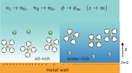
Figure 1: (Color online) Electric double layer containing small hydrophilic cations (Na⁺) and large hydrophobic anions (BPh${}_{4}^{+}$) in an aqueous mixture on a metal wall. There can be two kinds of ion distributions with a common potential drop $\Psi$, which coexist in certain conditions (see Figs.4-6). Gradation of solvent region represents water concentration.

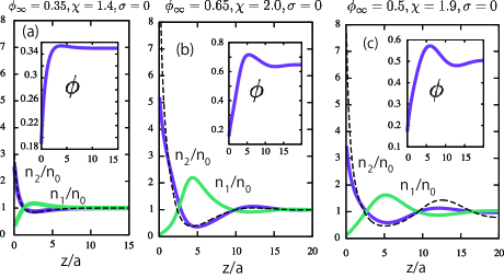
Figure 2: (Color online) Hydrophilic cations $n_{1}(z)$ and hydrophobic anions $n_{2}(z)$ next to hydrophobic wall for $\sigma=0$ with $n_{0}=4\times 10^{-3}v_{0}^{-1}$. Bulk water composition $\phi_{\infty}$ and interaction parameter $\chi$ are (a) $0.35$ and $1.4$, (b) $0.65$ and $2.0$, and (c) $0.5$ and $1.9$. Water profile $\phi(z)$ is also shown (insets). Anions are richer in the oil-rich adsorption layer. Steric effect due to finite sizes of ions are accounted for (bold lines). Broken lines represent anion profiles without steric effect ($v_{1}=v_{2}=0$).

The bulk free energy density is given by Oka ; Onuki ; Tsori ; Ben ; Bu ; Onukireview ; Nara ; Ciach ; Ben1 ; Leibler ; Roij

$$f = \frac{T}{v_{0}}(\phi\ln\phi+\phi^{\prime}\ln\phi^{\prime}+\chi\phi\phi^{\prime})+\frac{1}{2}C|\nabla\phi|^{2}$$ (3)

$$+\sum_{i=1,2}n_{i}[T\ln(n_{i}v_{i})-T+{\mu_{\rm sol}^{i}(\phi)}]+\frac{\varepsilon(\phi)}{2}|{\mbox{\boldmath$E$}}|^{2},$$

where $\chi$ is the interaction parameter depending on $T$ and we set $C=T/a$ Onukibook ; Safran . The $\mu_{\rm sol}^{i}$ is the solvation chemical potential, which is negative (positive) for hydrophilic (hydrophobic) ions. Its difference $\Delta\mu_{\rm sol}^{i}$ between coexisting two phases is the Gibbs transfer free energy (per ion), whose size is large ($\gg T)$ in aqueous mixtures in strong segregation Hung but is of order $T$ for water-alcohol in weak segregation Marcus . Here, we assume the linear form,

$$\mu_{\rm sol}^{i}(\phi)=-Tg_{i}\phi,$$ (4)

with $g_{1}=-g_{2}=10$. Then, $\Delta\mu_{\rm sol}^{i}\sim\pm 10T$ for strong segregation Hung . The last term in $f$ is the electrostatic part, where $\varepsilon$ is the dielectric constant and ${\mbox{\boldmath$E$}}=-\nabla\psi$ is the electric field. We assume the linear form $\varepsilon(\phi)=\varepsilon_{0}+\varepsilon_{1}\phi$ Debye with $\varepsilon_{0}=\varepsilon_{1}=e^{2}/12\pi aT$. The Bjerrum length is then $3a/(1+\phi)$. Most previous papers treated the simple case $v_{1}=v_{2}=v_{0}$ Ig ; Bazant ; Bike ; Andel , but some attempts were also made for the asymmetric case $v_{1}\neq v_{2}$ Maggs ; Bie .

The surface free energy density at $z=0$ is of the simple form $f_{s}=h_{1}\phi$, where $h_{1}$ is the surface field arising from the solvent-wall interactions Roth . Minimizing the total free energy $F=\int_{z>0}d{\mbox{\boldmath$r$}}f+\int_{z=0}dxdyf_{s}$ Roth , we find the boundary condition $\partial\phi/\partial z=h_{1}/C$ at $z=0$. Supposing a hydrophobic wall, we set $h_{1}=0.2T/a^{2}$ to obtain $\phi(z)=\phi(0)+0.2z/a+\cdots$ for small $z$.

The electric potential $\psi$ obeys the Poisson equation $\nabla\cdot\varepsilon\nabla\psi=e(n_{2}-n_{1})$, where $\psi\to 0$ as $z\to\infty$. Then, $\Psi\equiv\psi(0)$ is the potential drop across the layer, which is independent of $(x,y)$ on a metal surface. In this Letter, we control the surface charge $Q=\int dxdy~{}\sigma$, where $\sigma(x,y)$ is the charge density related to $\psi$ by

$$\sigma=-\varepsilon\partial\psi/\partial z\quad(z=0).$$ (5)

We calculated all the profiles assuming homogeneity of the chemical potentials $\mu_{\phi}=\delta F/\delta\phi$ and $\mu_{i}=\delta F/\delta n_{i}$ together with the Poisson equation for $z>0$. Here, $\mu_{\phi}$ and $\mu_{i}$ are determined by $\phi_{\infty}$ and $n_{0}$ (see their explicit expressions in SI Supp ).

We are not very close to the solvent criticality ($\chi=2$ and $\phi_{\infty}=0.5$) in the bulk. In its vicinity, a mesophase appears in the bulk with addition of an antagonistic salt Ciach ; Sada ; Onuki ; Onukireview ; Nara . We are also away from the solvent coexistence curve limiting ourselves to the case $\chi\leq 2$, so we do not discuss the wetting with ions Roij ; Bu ; Oka . In this situation, we first seek one-dimensional (1D) profiles fixing $\sigma$, where all the quantities depend only on $z$. For constant $\mu_{\phi}$ and $\mu_{i}$, we consider the grand potential density,

$$\omega=\int_{0}^{\infty}dz[f-\mu_{\phi}\phi-\sum_{i}\mu_{i}n_{i}+p_{\infty}]+h_{1}\phi(0).$$ (6)

where $p_{\infty}=\mu_{\phi}\phi_{\infty}+\sum_{i}\mu_{i}n_{0}-f(\infty)$. We then find

$$d\omega/d\sigma=\Psi,$$ (7)

at fixed $n_{0}$ and $\phi_{\infty}$ (see its derivation in SI Supp ). Thus $\Psi$ is the field variable conjugate to $\sigma$. We require $d\Psi/d\sigma>0$ for the thermodynamic stability.

For $\sigma=0$, local charge separation occurs due to the presence of an oil-rich adsorption layer on a hydrophobic wall. In Fig.2, the anions accumulate for $z<\ell_{1}\sim 3a$, while the cations are richer in the next layer $\ell_{1}<z<\ell_{2}\sim 7a$. In (a), it is relatively mild with $\phi_{\infty}=0.35$ and $\chi=1.4$, where the solvent is oil-rich at any $z$. However, it is more amplified in (b) and (c). Indeed, the deviation $\phi_{\infty}-\phi(z)$ is enlarged with $\phi_{\infty}=0.65$ and $\chi=2$ in (b), while the criticality is closer with $\phi_{\infty}=0.5$ and $\chi=1.9$ in (c). The normalized potential drop $e\Psi/T$ is (a) $-0.40$, (b) $-2.31$, and (c) $-1.16$. Furthermore, in (b) and (c), the deviations of $\phi$, $n_{i}$, and $\psi$ are strongly coupled even in the bulk, leading to oscillatory decays (as a precursor of the mesophase)Oka ; Ciach . In addition, $v_{2}n_{2}(0)\sim 0.1$ in (b). Thus, to check relevance of the steric effect, we also calculated $n_{2}(z)$ for $v_{1}=v_{2}=0$ Onukireview . The resultant $n_{2}(0)$ at $z=0$ is twice larger than that with the steric effect in (b) and (c), but is larger only by $20\%$ in (a). Notice that neutral colloidal particles in the same situation behave as negatively charged particles Faraudo1 .

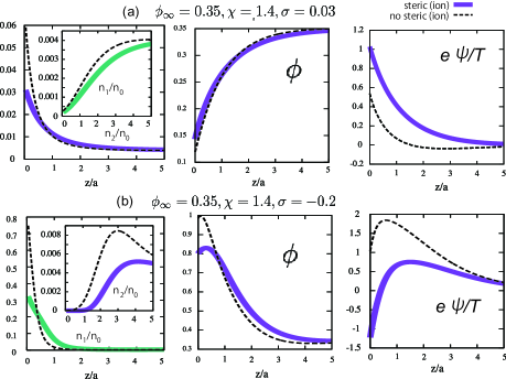
Figure 3: (Color online) 1D profiles of ions (left), $\phi(z)$ (middle), and $e\psi(z)/T$ (right) for $\sigma=0.03$ (top) and $-0.2$ (bottom) near a hydrophobic wall, where $\phi_{\infty}=0.35$ and $\chi=1.4$. These states are stable on the curve in Fig.4(a). Broken lines are obtained without steric effect ($v_{1}=v_{2}=0$).

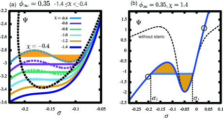
Figure 4: (Color online) Potential drop $\Psi$ vs surface charge density $\sigma$ (in units of $T/e$ and $e/a^{2}$, respectively) from 1D solutions for $\phi_{\infty}=0.35$, where (a) $\chi=-0.4,-0.6,-0.8,-1,-1.2$, and $-1.4$ and (b) $\chi=1.4$. From Eq.(9), first order phase transition occurs between two layer states at $\sigma=\sigma_{1}$ and $\sigma_{2}$. Two colored regions in yellow have the same area in (a) and (b). Two points ($\circ$) in (b) on the curve represent two states at $\sigma=-0.2$ and 0.03 in Fig.3. Dotted line in (b) represents $\Psi$ without steric effect ($v_{1}=v_{2}=0$).

In Fig.3, we give profiles of $n_{i}$, $\phi$, and $\psi$ for (a) $\sigma=0.03$ and (b) $\sigma=-0.2$, where $\phi_{\infty}=0.35$ and $\chi=1.4$ (see Fig.4(b) for the corresponding states). In (a), the anion accumulation is stronger than in Fig.2(a) (where $n_{2}(0)$ is 3 times larger) and the cations are expelled from the wall. In (b), the surface charge density $-0.2$ is largely negative, which is needed to induce cation accumulation at the hydrophobic wall. In (b), we then find $v_{1}n_{1}(0)\sim 0.15$, where $\phi(z)$ exceeds $\phi_{\infty}$ at any $z$. Here, $e\Psi/T$ is equal to (a) $1.0$ and (b) $-1.0$.

In Fig.4(a), we show $\Psi$ vs $\sigma$ for several $\chi$ at $\phi_{\infty}=0.35$. Here, $\Psi$ has local maximum and minimum as a function of $\sigma$ for $\chi>\chi_{c}=-1.243$. Generally, $\chi_{c}$ depends on $\phi_{\infty}$ and $n_{0}$. This indicates coexistence of two surface layers at $\sigma=\sigma_{1}$ and $\sigma_{2}$ with a common $\Psi(\sigma_{1})=\Psi(\sigma_{2})$ for $\chi>\chi_{c}$. Let the areas of these layers be $S_{1}$ and $S_{2}$, where $S=S_{1}+S_{2}$ is the total wall area. At fixed charge $Q=S_{1}\sigma_{1}+S_{2}\sigma_{2}$, we minimize the total grand potential,

$$\Omega=S_{1}\omega(\sigma_{1})+S_{2}\omega(\sigma_{2})-\lambda(S_{1}\sigma_{1}+S_{2}\sigma_{2}-Q),$$ (8)

with respect to $\sigma_{1}$, $\sigma_{2}$, and $S_{1}$. The $\lambda$ is the Lagrange multiplier. With the aid of Eq.(7) we find $\lambda=\Psi(\sigma_{1})=\Psi(\sigma_{2})$ and $\omega(\sigma_{1})-\lambda\sigma_{1}=\omega(\sigma_{2})-\lambda\sigma_{2}$. These yield

$$\omega(\sigma_{2})-\omega(\sigma_{1})=\int_{\sigma_{1}}^{\sigma_{2}}d\sigma\Psi(\sigma)=\Psi(\sigma_{1})(\sigma_{2}-\sigma_{1}).$$ (9)

which is a Maxwell rule Max . In (b), we then find $\sigma_{1}=-0.19$ and $\sigma_{2}=-0.014$ for $\chi=1.4$. See SI for results in the range $\sigma_{1}<\sigma<\sigma_{2}$ Supp .

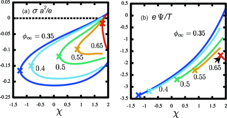
Figure 5: (Color online) Coexistence curves in (a) $\sigma$-$\chi$ plane and (b) $\Psi$-$\chi$ plane. for $\phi_{\infty}=0.35,0.4,0.5,0.55,$ and 0.65 at $n_{0}=4\times 10^{-3}v_{0}^{-1}$. For each $\phi_{\infty}$, two layers coexist inside the corresponding curve in (a), while $\Psi$ is a field variable common in coexisting two layers. Critical points are marked $(\times$).

In Fig.5, we display the coexistence curves in the $\chi$-$\sigma$ and $\chi$-$\Psi$ planes for several $\phi_{\infty}$. For each $\phi_{\infty}$, two layers coexist with $\sigma=\sigma_{1}$ and $\sigma_{2}$ inside the corresponding curve in (a), while $\Psi$ is common in these layers in (b). Critical points are reached as $\sigma_{2}-\sigma_{1}\to 0$, which form a critical line on the coexistence surface in the $\chi$-$\sigma$-$\phi_{\infty}$ (or $\chi$-$\Psi$-$\phi_{\infty}$) space (at fixed $n_{0}$). These phase behaviors are sensitive to $v_{1}$, $v_{2}$, and $h_{1}$, though the transition itself exists even for $v_{1}=v_{2}=0$.

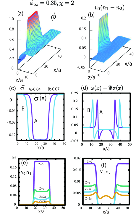
Figure 6: (Color online) Coexistence of two layers with $\sigma=0.02$ and $-0.14$ for $\phi_{\infty}=0.35$ and $\chi=2$ (see Fig.5). (a) $\phi(x,z)$ and (b) $v_{0}(n_{1}(x,z)-n_{2}(x,z))$ on the $zx$ plane. (c) $\sigma(x)a^{2}/e$ with ${\bar{\sigma}}=Q/S$ being (A) $-0.04$ and (B) $-0.07$ in units of $e/a^{2}$. (d) $[\omega(x)-\Psi\sigma(x)]a^{2}/T$ for (A) and (B). Cross-sectional profiles of (e) $v_{0}n_{1}(x,a)$ and (f) $v_{0}n_{2}(x,a)$ at $z/a=0,1,2$, and 3, exhibiting small peaks at boundaries for $z\geq a$.

We calculated 2D profiles from homogeneos $\mu_{\phi}$ and $\mu_{i}$ in the $zx$ plane with $\chi=2$ and $\phi_{\infty}=0.35$. For this $\phi_{\infty}$, the phase transition behavior is not much changed in the range $1.4\leq\chi\leq 2$ in Fig.5(a). In Fig.6, we show (a) $\phi$ and (b) $v_{0}(n_{1}-n_{2})$, where a stripe region with $\sigma=\sigma_{1}=-0.14$ is embedded between regions with $\sigma=\sigma_{2}=0.01$ at $\Psi=0.32$. Here, the mean surface charge density ${\bar{\sigma}}=Q/S$ is between $\sigma_{1}$ and $\sigma_{2}$. In (c), $\sigma(x)$ from Eq.(5) is roughly equal to $\sigma_{1}$ or $\sigma_{2}$ except for the boundary regions. The fraction of the region with $\sigma=\sigma_{1}$ is nicely given by $(\sigma_{2}-{\bar{\sigma}})/(\sigma_{2}-\sigma_{1})$. In (d), we plot ${\hat{\omega}}(x)\equiv\omega(x)-\Psi\sigma(x)$, where $\omega$ is defined in Eq.(6). From Eq.(9) it assumes a nearly common value ${\hat{\omega}}_{1}$ in the two regions. The integral of ${\hat{\omega}}(x)-{\hat{\omega}}_{1}$ across one of the boundary regions is the line tension $\tau$ Line , which is of order $0.1T/a$ here. In (e) and (f), cross-sectional profiles of $n_{1}$ and $n_{2}$ at constant $z$ are given, which exhibit small peaks at the boundaries slightly away from the wall. This is because of the Coulomb attraction between the cations and the anions which are locally separated across the boundaries. For the same reason, more marked peaks appear in the densities of antagonistic ion pairs near water-oil interfaces Luo ; Onukireview ; Onuki .

We propose experiments in the above situation. Let $\bar{\sigma}$ be decreased slightly below $\sigma_{2}$ on a hydrophobic metal wall. Then, the oil-rich layer with hydrophobic anions becomes metastable against formation of small water-rich regions with hydrophilic cations. For a finite line tension $\tau$, their shapes are circular with the critical radius Onukibook

$$r_{c}=\tau/[(d\Psi/d\sigma)(\sigma_{2}-{\sigma}_{1})(\sigma_{2}-{\bar{\sigma}})],$$ (10)

where the derivative $d\Psi/d\sigma$ is taken at $\sigma=\sigma_{2}$. On the other hand, a hydrophilic metal wall will be covered with a water-rich layer for $\sigma\cong 0$, but small oil-rich regions will be nucleated with increasing $\sigma>0$.

In summary, we have found a first-order surface transition with antagonistic ion pairs having different sizes. In future, we should examine wetting near the solvent coexistence curve with an antagonistic salt. We will study behavior of colloidal particles (including Janus ones) in a mixture solvent with an antagonistic salt, where the ion distributions around them can be very complex.

Supplemental Information
Electric double layer composed of an antagonistic salt in an aqueous mixture:
      Local charge separation and surface phase transition
                           Shunsuke Yabunaka^a and Akira Onuki^b
a Fukui Institute for Fundamental Chemistry, Kyoto University, Kyoto 606-8103, Japan
^b Department of Physics, Kyoto University, Kyoto 606-8502, Japan

Space-filling condition and chemical potentials
We introduce the ion volumes $v_{1}$ and $v_{2}$ using their definittion in Eq.(2) in our Letter. The total volume fraction $\phi_{\rm tot}$ is the sum of those of water, oil, cations, and anions:

$$\phi_{\rm tot}=\phi+\phi^{\prime}+v_{1}n_{1}+v_{2}n_{2}.$$ (S.1)

where $v_{0}$, $v_{1}$, and $v_{2}$ depend on $T$ and $p$ but not on the mole fractions of the four components. We assume that $\phi_{\rm tot}$ is very close to 1 even for not very small $v_{1}n_{1}+v_{2}n_{2}$. Its deviation from 1 should yield an increase in the Helmholtz free energy $\Delta F=\int_{z>0}d{\mbox{\boldmath$r$}}\Delta f$ with

$$\Delta f=\gamma(\phi_{\rm tot}-1)^{2}/2v_{0},$$ (S.2)

where $\gamma$ is a large coefficient ($\gg T$). If the fluid is homogeneous with volume $V$, the excess free energy is $\Delta F=\gamma(V-V_{\rm tot})^{2}/2Vv_{0}$ with $V_{\rm tot}=V\phi_{\rm tot}=v_{0}(N_{\rm w}+N_{\rm o})+v_{1}N_{1}+v_{2}N_{2}$, where $N_{\alpha}$ ($\alpha={\rm w},\rm{o},1$, and 2) are the total particle numbers. Its differentiation with respect to $V$ at fixed $N_{\alpha}$ gives the excess pressure,

$$\Delta p=\gamma(\phi_{\rm tot}-1)/v_{0}.$$ (S.3)

We treat physical states with $|\Delta p|\ll T/v_{0}$. If $\gamma\gg T$, the isothermal compressibility (at fixed molar fractions) is nearly equal to $v_{0}/\gamma$. It is worth noting that the compressibility of ambient liquid water (300 K and 1 atm) is $4.5\times 10^{-4}/$MPa $\sim 0.06v_{0}/T$ for $a=v_{0}^{1/3}=3~{}{\rm\AA}$.

If we allow small deviations of the space-filling condition (1), we should replace the total free energy $F=\int_{z>0}d{\mbox{\boldmath$r$}}f+\int_{z=0}dxdy~{}h_{1}\phi$ by $F+\Delta F$. With the aid of Eqs.(3) and (4), the chemical potentials are defined by ${\hat{\mu}}_{\alpha}=\delta(F+\Delta F)/\delta n_{\alpha}$ ($\alpha={\rm w},\rm{o},1$, and 2), where $F+\Delta F$ is treated as a functional of $n_{\rm w}$, $n_{\rm{o}}$, $n_{1}$, and $n_{2}$ at fixed $T$ and surface charge $Q=\int dxdy\sigma$. To calculate these quantities we consider small variations $\delta\phi$, $\delta n_{i}$, and $\delta\sigma$. Using $\delta(\varepsilon|{\mbox{\boldmath$E$}}|^{2})=-|{\mbox{\boldmath$E$}}|^{2}\delta\varepsilon+2{\mbox{\boldmath$E$}}\cdot\delta(\varepsilon{\mbox{\boldmath$E$}})$ and

$$\int_{z>0}d{\mbox{\boldmath$r$}}{\mbox{\boldmath$E$}}\cdot{\delta(\varepsilon{\mbox{\boldmath$E$}})}=\int_{z>0}d{\mbox{\boldmath$r$}}~{}\psi e(\delta n_{1}-\delta n_{2})+\int_{z=0}dxdy~{}\psi\delta(\varepsilon E_{z}),$$ (S.4)

we obtain the incremental change in $F+\Delta F$ as

$$\delta(F+\Delta F)=\int_{z>0}d{\mbox{\boldmath$r$}}\sum_{\alpha={\rm w},\rm{o},1,2}{\hat{\mu}}_{\alpha}\delta n_{\alpha}+\int_{z=0}dxdy\bigg{[}(h_{1}-C\partial\phi/\partial z)\delta\phi+\psi\delta(\varepsilon E_{z})\bigg{]},$$ (S.5)

Then, since $\delta D_{z}=\delta\sigma$ and $C\partial\phi/\partial z=h_{1}$ at $z=0$, the second term in Eq.(S.5) simply becomes $\Psi\delta Q$ on a metal surface with $\Psi=\psi(0)$ for $\phi(\infty)=0$. Some calculations give

$${\hat{\mu}}_{\rm w} = T[\ln\phi+1+\chi\phi^{\prime}-v_{0}\sum_{i}g_{i}n_{i}-\frac{Cv_{0}}{T}\nabla^{2}\phi]-\frac{v_{0}\varepsilon_{1}}{2}|{\mbox{\boldmath$E$}}|^{2}+\gamma(\phi_{T}-1),$$ (S.6)

$${\hat{\mu}}_{\rm o} = T[\ln\phi^{\prime}+1+\chi\phi]+\gamma(\phi_{T}-1),$$ (S.7)

$${\hat{\mu}_{1}} = T[\ln(n_{1}v_{1})-g_{1}\phi]+{e\psi}+\gamma(\phi_{T}-1)v_{1}/v_{0},$$ (S.8)

$${\hat{\mu}_{2}} = T[\ln(n_{2}v_{2})-g_{2}\phi]-{e\psi}+\gamma(\phi_{T}-1)v_{2}/v_{0}.$$ (S.9)

For equilibrium and metastable profiles, these chemical potentials are homogeneous constants. Using these profiles, we consider the grand potential defined by

$$\hat{\Omega}=\int_{z>0}d{\mbox{\boldmath$r$}}\bigg{[}f+\Delta f+p_{\infty}-\sum_{\alpha}{\hat{\mu}}_{\alpha}n_{\alpha}\bigg{]}+\int_{z=0}dxdy~{}h_{1}\phi,$$ (S.10)

where $p_{\infty}$ is a constant chosen to make the integrand in the first term vanish for large $z$. Then, from $C\partial\phi/\partial z=h_{1}$ at $z=0$ and Eq.(S.5), we obtain

$$\delta\hat{\Omega}=\Psi\delta Q.$$ (S.11)

If $\hat{\Omega}$ is treated as a function of $Q$, we obtain $d{\hat{\Omega}}/dQ=\Psi$ for each $\phi_{\infty}$, $n_{0}$, and $T$. As $\phi_{\rm tot}\to 1$ in the one-dimensional case, $\hat{\Omega}$ in Eq.(S.10) tends to $S\omega$, where $\omega$ is defined by Eq.(6) and $S$ is the surface area of the metal wall. Then, we find $d\omega/d\sigma=\Phi$ in Eq.(7).

Below Eq.(5) of our Letter, we have introduced $\mu_{\phi}=\delta F/\delta\phi$ and $\mu_{i}=\delta F/\delta n_{i}$ starting with Eq.(1) ($\phi_{\rm tot}=1$), where $\phi^{\prime}$ is eliminated and $F$ is a function of the three variables $\phi$, $n_{1}$, and $n_{2}$. For small $\phi_{\rm tot}-1$ and large $\gamma/T$, we can express $\mu_{\phi}$ and $\mu_{i}$ as

$$\mu_{\phi}=({\hat{\mu}}_{\rm w}-{\hat{\mu}}_{\rm o})/v_{0},\quad~{}\mu_{i}={\hat{\mu}}_{i}-{\hat{\mu}}_{\rm o}v_{i}/v_{0}\quad(i=1,2),$$ (S.12)

where the terms proportional to $\gamma(\phi_{\rm tot}-1)$ are eliminated.

Changeover of layer profiles
In our Letter, we have presented numerical results for $\phi_{\infty}=0.35$ and $n_{0}=4\times 10^{-3}v_{0}^{-1}$ at $\chi=1.4$ on a hydrophobic wall in Figs.2-4. Here, adopting these parameter values, we give 1D profiles of (a) $n_{1}(z)$, (b) $n_{2}(z)$, (c) $\phi(z)$, and (d) $\psi(z)$ in dimensionless units in Fig.S1. We set $\sigma$ equal to (A) $0$, (B) $-0.04$, (C) $-0.08$, (D) $-0.12$, and (E) $-0.16$ in units of $e/a^{2}$, where $v_{0}=a^{3}$. These quantities largely change with decreasing $\sigma$. In (a), the cations are expelled from the wall for $\sigma=0$, but they abruptly accumulate near the wall for $\sigma\lesssim-0.08$ because of their small size $v_{1}=0.5v_{0}$. In (b), the anions are accumulated near the wall with $v_{2}n_{2}(0)\cong 0.05$ for $\sigma=0$, but are expelled from the wall for $\sigma\gtrsim-0.08$. The anions accumulate more weakly than the cations because of their large size ratio $v_{2}/v_{1}=10$. In (c), the water volume fraction $\phi(z)$ is less than $\phi_{\infty}$ near the wall for $\sigma=0$ and -0.04, but is increased above $\phi_{\infty}$ for the lower $\sigma$ values. In (d), the potential drop $\Psi=\psi(0)$ remains negative, but $\psi(z)$ gradually increases near the wall. For $\sigma\lesssim-0.08$, $\psi(z)$ exhibits a maximum at an intermediate $z_{m}\sim 1.5a$, so the electric field $E_{z}=-d\psi/dz$ is positive for $z<z_{m}$ and negative for $z>z_{m}$.

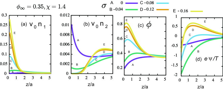
Figure S7: (Color online) Changeover of profiles of (a) $v_{0}n_{1}(z)$, (b) $v_{0}n_{2}(z)$, (c) $\phi(z)$, and (d) $e\psi(z)/T$ for five values of $\sigma$, where $\chi=1.4$, $\phi_{\infty}=0.35$, and $n_{0}=4\times 10^{-3}v_{0}^{-1}$.

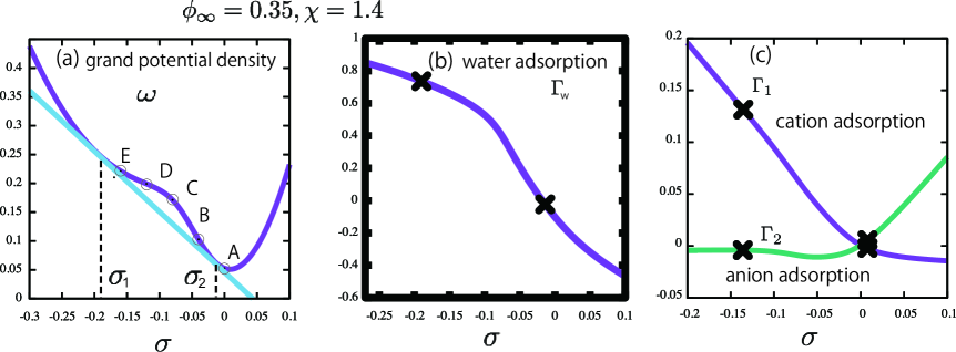
Figure S8: (Color online) (a) $\omega a^{2}/T$, (b) $\Gamma_{\rm w}a^{2}$, and (c) $\Gamma_{i}a^{2}$ ($i=1,2$) as functions of $\sigma$ (in units of $e/a^{2}$). First order phase transion occurs between two states at $\sigma=\sigma_{1}=-0.19$ and $\sigma=\sigma_{2}=-0.014$. In (a) points A, B, …., and E correspond to those in Fig.S1. In (b) and (c) these points are marked by $\times$. The other parameter values are the same as those in Fig.S1.

For the parameter values in Fig.S1, a first order phase transition occurs between two surface charge densities given by $\sigma_{1}=-0.19$ and $\sigma_{2}=-0.014$ from Fig.4(b). In Fig.S2(a), the grand potential density $\omega(\sigma)$ in Eq.(6) is plotted, where its tangential line at $\sigma=\sigma_{1}$ and that at $\sigma=\sigma_{2}$ coincide from Eq.(9) with a common slope equal to the potential drop $\Psi$. Thus, the state (A) is stable where $\sigma>\sigma_{2}$. However, the states (B)-(E) are metastable or unstable because their $\sigma$ values are between $\sigma_{1}$ and $\sigma_{2}$. In (b) and (c), we plot the excess adsorbates $\Gamma_{\rm w}$, $\Gamma_{1}$, and $\Gamma_{2}$ for water molecules, cations, and anions, respectively. In our semi-infinite case they are defined by

$$\Gamma_{\rm w}=v_{0}^{-1}\int_{0}^{\infty}dz[\phi(z)-\phi_{\infty}],\quad\quad\Gamma_{i}=\int_{0}^{\infty}dz[n_{i}(z)-n_{0}]\quad(i=1,2).$$ (S.13)

With decreasing $\sigma$, $\Gamma_{\rm w}$ and $\Gamma_{1}$ increase, while $\Gamma_{2}$ decreases to zero, which confirms the strong coupling between the composition and the ion densities.

References

(1) J. N. Israelachvili,
Intermolecular and Surface Forces
(Academic Press, London, 1991).
(2)
H.-J. Butt, K. Graf, and M. Kappl, Physics and Chemistry of Interfaces,
3rd ed. (Wiley-VCH Verlag GmbH, Weinheim, 2013).
(3) M. Z. Bazant, M. S. Kilic, D. Storey, and A. Ajdari,
Adv. Colloid Interface Sci.152, 48 (2009).
(4)
D. Ben-Yaakov, D. Andelman, R. Podgornik, and D. Harries, Curr. Opin.
Colloid Interface Sci. 16, 542 (2011)
(5)
A. Onuki, Phys. Rev. E 73, 021506 (2006).
(6) D. Ben-Yaakov, D. Andelman,
D. Harries, and R. Podgornik,
J. Phys. Chem. B 113, 6001 (2009).
(7) R. Okamoto and A. Onuki,
Phys. Rev. E 84, 051401 (2011).
(8) A. Onuki, R. Okamoto, and T. Araki.
Bull. Chem. Soc. Jpn 84, 569 (2011).
(9) Y. Tsori and L. Leibler, Proc. Natl Acad. Sci.
104, 7348 (2007).
(10) J. C. Everts, S. Samin, and R. van Roij,
Phys. Rev. Lett. 117, 098002 (2016).
(11) S. Samin and Y. Tsori,
J. Chem. Phys. 136, 154908 (2012);
Y. Katsir and Y. Tsori,
J. Phys.: Condens. Matter 29, 063002 (2017).
(12)
A. Onuki, S. Yabunaka, T. Araki, R. Okamoto,
Curr. Opin. Colloid Interface Sci.
22, 59 (2016).
(13)
A. Onuki, T. Araki and R. Okamoto,
J. Phys.: Condens. Matter 23,284113 (2011).
(14) F. Pousaneh and A. Ciach,
Soft Matter 10, 8188 (2014).
(15) K. Sadakane, H. Seto, H. Endo, and M. Shibayama,
J. Phys. Soc. Jpn. 76, 113602 (2007).
(16)
K. Sadakane, A. Onuki, K. Nishida, S. Koizumi, and H. Seto,
Phys. Rev. Lett. 103, 167803 (2009);
K. Sadakane, M. Nagao, H. Endo, and H. Seto,
J. Chem. Phys. 139, 234905 (2013).
(17) J. Leys,
D. Subramanian, E. Rodezno, B. Hammouda, and M. A. Anisimov,
Soft Matter 9, 9326 (2013).
(18) R. Schurhammer and G. Wipff,
J. Phys. Chem. A 104, 11159 (2000).
The shape of BPh is nonspherical.
However, if we treat the volume of a phenil ring
to be close to that of
a water molecule, we roughly obtain
.
(19) D. Chandler, Nature 640 (2005).
(20)
S. Rajamani, T. M. Truskett, and S. Garde, PNAS 102, 9475 (2005).
(21)
G. Luo, S. Malkova, J. Yoon, D. G. Schultz, B. Lin, M.
Meron, I. Benjamin, P. Vanysek, and M. L. Schlossman,
Science, 311, 216 (2006).
(22) M. Michler, N. Shahidzadeh, M. Westbroek,
R. van Roij, and D. Bonn, Langmuir 31, 906 (2015).
(23) E. Leontidis, Curr. Opin.
Colloid Interface Sci.23, 100 (2016).
(24)
D. Bastos-Gonzlez, L. Prez-Fuentes,
C. Drummond, J. Faraudo,
Curr. Opin. Colloid Interface Sci.23, 19 (2016).
(25) C. Calero and J. Faraudo,
D. Bastos-Gonzlez,
J. Am. Chem. Soc. 133, 15025 (2011).
(26) O. Stern, Z. Elektrochem. 30, 508 (1924).
(27) J. J. Bikerman, Philos. Mag. 33, 384 (1942);
V. Freise, Z Elektrochem 56, 822 (1952);
M. Eigen and E. Wicke, J. Phys. Chem. 58, 702 (1954).
(28)
V. Kralj-Iglic and A. Iglic, J. Phys. II 6, 477 (1996).
(29) I. Borukhov, D. Andelman, and H. Orland, Phys. Rev. Lett.
79, 435 (1997).
(30) V. L. Shapovalov and G. Brezesinski,
J. Phys. Chem. B 110, 10032 (2006).
(31) P. Biesheuvel and M. van Soestbergen, J. Colloid Interface
Sci. 316, 490 (2007).
(32) A. C. Maggs and R. Podgornik,
Soft Matter 12, 1219 (2016).
(33)
P. J. Flory, Principles of Polymer Chemistry (Cornell Univ.
Press, Ithaca, 1953), Chaps. 12 and 13.
In polymer mixtures, the density of component
multiplied by its polymerization index
is equal to its volume fraction
divided by the common monomer volume .
They are assumed to satisfy .
(34)
We may use the the Mansoori-Carnahan-Starling-Leland
model for high-density liquid mixtures Bazant ; Bie ; Maggs
to justify Eq.(1), where
and are determined by
the hard-core part of the free energy
as functions of and .
(35) See Supplemental Information.
(36) L.Q. Hung,
J. Electroanal Chem. 115, 159 (1980);
J. Koryta, Electrochim. Acta 29, 445 (1984).
T. Osakai and K. Ebina,
J. Phys. Chem. B 102, 5691 (1988).
(37) C. Kalidas, G. Hefter, and Y. Marcus,
Chemical Rev. 100, 819 (2000).
(38) A. Onuki
Phase Transition Dynamics
(Cambridge University Press,Cambridge, 2002).
(39) The coefficient in Eq.(3) depends on
the microscopic interactions and can be determined
from experimental data of the correlation length
or the surface tension.
(40) P. Debye and K. Kleboth, J. Chem. Phys. 42, 3155 (1965).
These authors treated a binary mixture,
where the linear form
fairly holds.
(41) J. W. Cahn. J. Chem. Phys. 66,
3667 (1977); D. Bonn and D. Ross, Rep. Prog. Phys.
64, 1085 (2001).
(42) For one-component fluids
the chemical potential depends on the density
at fixed where is the Helmholtz
free energy density. When a gas with density and a liquid with
density coexist, we have
analogously to Eq.(9).
(43) B. Widom, J. Phys. Chem. 99, 2803 (1995).