Visual guide to optical tweezers

Abstract

It is common to introduce optical tweezers using either geometric optics for large particles or the Rayleigh approximation for very small particles. These approaches are successful at conveying the key ideas behind optical tweezers in their respective regimes. However, they are insufficient for modelling particles of intermediate size and large particles with small features. For this, a full field approach provides greater insight into the mechanisms involved in trapping. The advances in computational capability over the last decade has led to better modelling and understanding of optical tweezers. Problems that were previously difficult to model computationally can now be solved using a variety of methods on modern systems. These advances in computational power allow for full field solutions to be visualised, leading to increased understanding of the fields and behaviour in various scenarios. In this paper we describe the operation of optical tweezers using full field simulations calculated using the finite difference time domain method. We use these simulations to visually illustrate various situations relevant to optical tweezers, from the basic operation of optical tweezers, to engineered particles and evanescent fields.

Preprint of:
Isaac C. D. Lenton, Alexander B. Stilgoe, Halina Rubinsztein-Dunlop and Timo A. Nieminen
“Visual guide to optical tweezers”
European Journal of Physics 38(3), 034009 (2017)
https://doi.org/10.1088/1361-6404/aa6271

 

1 Introduction

Development of optical tweezers began in the second half of the 20th centry with the first demonstrations of optical levitation in 1971 and the single beam gradient trap in 1986 [1, 2]. It had long been known that light could influence the trajectories of particles, proposals for solar sails had been recorded as early as 1924 [3], but the small momentum carried by photons ($\hbar\omega/c$ per photon, compared to $\hbar\omega$ energy, where $\omega$ is the optical angular frequency and $c$ is the speed of light in free space) made experimental demonstrations of optical forces difficult without high intensity light sources. The invention of the laser in 1960 likely contributed to the realisation of optical levitation and optical tweezing by allowing high intensity spatially confined beams to be used in experiments. Since their invention, optical tweezers have seen applications to various fields ranging from microbiology where they are used to trap and manipulate cells and DNA to microfluidics where diffractive optical elements can be combined with optical tweezers to measure properties of fluids such as viscosity and elasticity [4, 5, 6].

The concepts behind the operation of optical tweezers are often introduced using either geometric optics suitable for large spherical particles [2] or the Rayleigh approximation for small dipole-like particles [2]. Both these methods can provide important insight into the basic principles behind optical tweezers. In particular, both give a picture where the optical force can be separated into a gradient force and a scattering force. The Rayleigh approximation assumes particles are much smaller than the illumination wavelength. In this regime the particle are modelled as a single scattering dipole. for which there are analytical solutions. The geometric optics approach works well for large particles where interference effects and minimum beam radius can be ignored. Reference [7] has some very nice animations and figures generated using geometric optics; their toolkit is suitable for teaching OT. However, for intermediate particles, large particles with small features or trapping involving evanescent fields, the full electromagnetic fields give much greater insight into the operation of optical tweezers.

Apart from a few specific cases for certain regimes, there are no analytical models for optical tweezers or the fields in/around arbitrary particles. As such, numerical modelling is an important tool for the design and analysis of tweezers experiments [8], good agreement between experimental and computational results has been demonstrated [9, 10]. Computational modelling of optical tweezers involves calculating how light is scattered by a trapped object in order to calculate forces, torques and other properties of interest. The advances in computational power and availability of codes and algorithms for modelling optical tweezers in the recent decade has led to increased ability to model optical tweezers. Many methods exist for performing scattering calculations [11]. However, many of the codes implementing these methods are not directly applicable to optical tweezers problems because they either don’t calculate properties of interest to optical tweezers or they make assumptions such as plane wave illumination [12].

The advances in computational capability and the availability of suitable codes for simulating optical tweezers has led to better models of optical tweezers. Some of these methods had been previously developed but suitable codes for modelling optical tweezers situations with suitable illumination have not always been available. Every numerical method has a unique set of advantages and limitations; a brief review of methods used by our group can be found in [13]. Our group currently uses a range of methods to simulate optical tweezers including the discrete dipole approximation, finite difference frequency domain and various Generalized Lorenz–Mie Theory and point matching methods. We have recently developed a finite difference time domain (FDTD) implementation, which solves Maxwell’s equations in the time domain by calculating discrete differences of the fields. FDTD is convenient for visualising the fields since the full fields are calculated as a convenient consequence of the method.

For this work, FDTD was chosen as this method gives the real fields and can easily simulate arbitrary geometries and inhomogeneous dielectric and conductive materials. Commercial FDTD tools are available that can be configured to simulate optical tweezers but our group has been developing our own FDTD package which we hope to release as open source software. The benefits of having an open source package are the ability to modify and configure the code in order to allow testing of new methods and calculation of properties of interest. The core components to the FDTD implementation are fairly straightforward; 2-D or 3-D implementations used as a learning tool or the development of a 2-D implementation as a guided exercise could make interesting educational tools.

The remainder of this paper is split into three parts. Section 2 provides an overview of optical tweezers including explanations of their operation using the Rayleigh approximation, geometric optics approach and full field simulations. Section 3 briefly describes FDTD and the types of illumination commonly used for optical tweezers. Finally, section 4 presents various simulations generated using FDTD which illustrate different optical trapping scenarios.

2 Optical tweezers

An optical tweezers experiment requires: a light source, such as a tightly focussed laser beam; a system to be investigated, such as a particle suspended in water; and a detection system to measure the properties of interest. A typical optical tweezers apparatus is shown in figure 1-A. This apparatus consists of a microscope system with the optical trapping beam introduced through the microscope objective. The particle to be trapped is located on a microscope slide between the microscope objective and the condenser. This kind of system allows the position of the particle to be directly imaged or the position to be inferred from the deflection of the trapping beam after passing through the system. Detection systems include quadrant photodiodes, high resolution cameras and position sensitive detectors. The system can be extended to include multiple optical traps by using multiple light sources, by time-sharing a beam over multiple locations with an acousto-optic modulator or by splitting the beam with diffractive or reflective optical elements such as a digital micro-mirror device or spatial light modulator [14]. In addition to the system shown in figure 1-A, other optical trapping systems may involve the use of evanescent fields or optical fibres or a combination of multiple systems depending on the problem requirements.

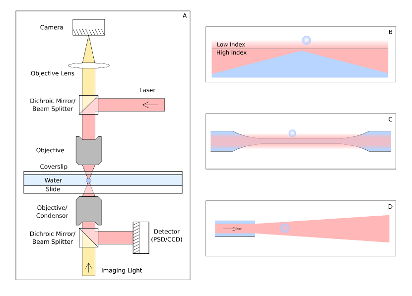
Figure 1: (A), a typical optical tweezers apparatus. (B), a particle in an evanescent field near the interface of a high/low index material. (C) a particle in an evanescent field from a tapered optical fibre. (D) a fibre based optical tweezers system.

There are multiple forces present in a typical optical tweezers system; in addition to the optical force from the trapping beam other forces from gravity, buoyancy, Brownian motion or other properties of the fluid might also apply [13].

2.1 Full field simulation and visualisation

There are two convenient starting points for calculation of optical forces in a full field simulation: an electromagnetic force law (e.g., the Lorentz force law), and the momentum flux density (the Maxwell stress tensor). We will begin with the first of these. The force density $\mathbf{f}$ exerted by electromagnetic fields on matter is, according the Lorentz force law:

$$\mathbf{f}=\rho\mathbf{E}+\mathbf{J}\times\mathbf{B},$$ (1)

where the force density is given by the forces acting on the charge density, $\rho$, and the current density, $\mathbf{J}$. For a dielectric particle such as is typically trapped in optical tweezers, we can replace the dielectric polarisation $\mathbf{P}$ per unit volume by its equivalent charge density $\rho=-\nabla\cdot\mathbf{P}$, and the polarisation current $\mathrm{d}\mathbf{P}/\mathrm{d}t$, the Lorentz force law becomes

$$\mathbf{f}=(\mathbf{P}\cdot\nabla)\mathbf{E}+\frac{\mathrm{d}\mathbf{P}}{\mathrm{d}t}\times\mathbf{B}.$$ (2)

We can then use the identity $(\mathbf{E}\cdot\nabla)\mathbf{E}=\nabla(\mathbf{E}\cdot\mathbf{E})/2-\mathbf{E}\times(\mathbf{E}\times\mathbf{E})$, the relationship between $\mathbf{P}$ and $\mathbf{E}$, $\mathbf{P}=(\epsilon-\epsilon_{0})\mathbf{E}$, where $\epsilon$ and $\epsilon_{0}$ are the permittivity of the particle and of free space, respectively, and the Maxwell equations [15] to obtain

$$\mathbf{f}=(\epsilon-\epsilon_{0})\left(\frac{1}{2}\nabla(\mathbf{E}\cdot\mathbf{E})+\frac{\mathrm{d}}{\mathrm{d}t}(\mathbf{E}\times\mathbf{B})\right).$$ (3)

A similar force also acts on the surrounding medium, if it has a permittivity different from $\epsilon_{0}$, and we must account for the force from contact with the surrounding medium. This gives an effective force density is

$$\mathbf{f}=(\epsilon_{\mathrm{particle}}-\epsilon_{\mathrm{medium}})\left(\frac{1}{2}\nabla(\mathbf{E}\cdot\mathbf{E})+\frac{\mathrm{d}}{\mathrm{d}t}(\mathbf{E}\times\mathbf{B})\right).$$ (4)

2.1.1 Rayleigh approximation

For the case where a particle is much smaller than the wavelength (a Rayleigh particle), the applied field can be assumed to be uniform over the particle, allowing us to very easily integrate the force density over the particle to find the total force:

$$\mathbf{F}=\mathbf{f}V,$$ (5)

where $V$ is the volume of the particle. For a sphere of radius $a$, $V=(4/3)\pi a^{3}$, and we can express the total force in terms of a polarisability $\alpha$:

$$\mathbf{F}=\alpha\left(\frac{1}{2}\nabla(\mathbf{E}\cdot\mathbf{E})+\frac{\mathrm{d}}{\mathrm{d}t}(\mathbf{E}\times\mathbf{B})\right).$$ (6)

The static polarisability of a sphere,

$$\alpha_{\mathbf{static}}=4\pi\epsilon_{\mathrm{medium}}a^{3}\left(\frac{\epsilon_{\mathrm{particle}}/\epsilon_{\mathrm{medium}}-1}{2\epsilon_{\mathrm{particle}}/\epsilon_{\mathrm{medium}}+1}\right),$$ (7)

is a good starting approximation for the polarisability $\alpha$. For a time-harmonic incident field, the time-averaged force is

$$\langle\mathbf{F}\rangle=\frac{1}{2}\mathrm{Re}\left\{\alpha\left(\frac{1}{2}\nabla(\mathbf{E}_{0}\cdot\mathbf{E}_{0}^{\ast})-2\mathrm{i}\omega\mathbf{E}_{0}\times\mathbf{B}_{0}^{\ast}\right)\right\}.$$ (8)

The first term, proportional to the gradient of the irradiance, is the gradient force, and the second term, proportional to the Poynting vector, is the scattering force. Using the static polarisability leads to a time-averaged scattering force of zero (because the polarisability is real). However, a time-harmonic dipole moment of amplitude $\mathbf{p}_{0}$ radiates an average power of $c^{2}Zk^{4}\mathbf{p}_{0}\cdot\mathbf{p}_{0}^{\ast}/(12\pi)$, where $k=2\pi/\lambda$ is the wavenumber and $Z$ the impedance of the medium, the polarisability must have an imaginary component. From the radiated power, the imaginary component of the polarisability must be

$$\mathrm{Im}(\alpha)=-\frac{cZk^{3}}{6\pi}|\alpha|^{2},$$ (9)

giving the required scattering force. For non-spherical Rayleigh particles, the appropriate static polarisability tensor can be used, correcting for radiated power.

Giving a simple analytical expression for the force on a trapped particle, depending only on the local values of the electromagnetic field and derivatives, the Rayleigh approximation can provide much useful insight into the optical trapping of small particles, such as the relative scaling of the gradient force, scattering force, and Brownian motion [2]. However, it is only quantitatively accurate for very small particles. In principle, we could integrate the effective force density given by (4) over the volume of the particle. We can also approach the problem differently, in terms of the momentum flux density, as given by the Maxwell stress tensor (MST).

2.1.2 Maxwell stress tensor

A general approach to calculating the optical force on a region involves integration of the Maxwell stress tensor and Poynting vector over a surface/volume surrounding the particle [8]

$$\mathbf{F}=\int_{S}\bar{\mathbf{T}}\cdot\mathrm{d}\mathbf{S}-\epsilon\mu\frac{\mathrm{d}}{\mathrm{d}t}\int_{V}\mathbf{U}\mathrm{d}V$$ (10)

where $S$ is a surface surrounding the volume, $V$, containing the particle; $\mathbf{U}$ is the Poynting vector and $\bar{\mathbf{T}}$ is the MST which can be defined using the Kronecker delta function $\delta_{ij}$ as

$$\bar{\mathbf{T}}_{ij}=\epsilon\mathbf{E}_{i}\mathbf{E}_{j}+\mu\mathbf{H}_{i}\mathbf{H}_{j}-\frac{1}{2}\left(\epsilon|\mathbf{E}|^{2}+\mu|\mathbf{H}|^{2}\right)\delta_{ij}.$$ (11)

The above equation gives the sum of the electromagnetic force acting on object contained in the volume and the rate of change of electromagnetic momentum within the volume. For a time-harmonic field, we can eliminate this second part by taking the time average, then (10) reduces to

$$\langle\mathbf{F}\rangle=\int_{S}\langle\bar{\mathbf{T}}\rangle\cdot\mathrm{d}\mathbf{S}.$$ (12)

Almost always, we wish to know the time-averaged force rather than the instantaneous electromagnetic force, so there is no practical loss of generality. The force can also be calculated using a similar volume integral form

$$\langle\mathbf{F}\rangle=\int_{V}\nabla\cdot\langle\bar{\mathbf{T}}\rangle\mathrm{d}V$$ (13)

where $\nabla\cdot\langle\bar{\mathbf{T}}\rangle$ denotes the divergence of the MST. For a particle in continuous wave illumination, this formula gives the average force when the time average is taken over one complete optical cycle.

For pulsed illumination, such as when using a femtosecond laser, the time average needs to be taken over a complete pulse. To calculate the average optical force on the particle the MST integral needs to be evaluated at multiple time steps. For a continuous wave source, the time average need only be taken over multiple samples from a single optical cycle. The error in the time average typically scales better than $1/m$ where $m$ is the number of samples. We have found that for most cases $m=3$ produces satisfactory results.

2.1.3 Geometric optics

We have not specified the surface of integration for (12). In principle, any surface enclosing the particle of interest, and containing nothing else experiencing a net force from the beam, can be used. A particular simple choice for a focussed beam. For such a beam, a well-defined far field exists, where the beam becomes a spherical wave. Taking the far field limit, it is convenient to use a spherical coordinate system $(r,\theta,\phi)$ for the calculation, since our surface area element $\mathrm{d}\mathbf{S}=r^{2}\mathrm{d}\theta\mathrm{d}\phi$, and radial components of the electromagnetic field can be neglected, and our integral reduces to

$$\mathbf{F}=-\int_{S}\frac{1}{2}\left(\epsilon|\mathbf{E}|^{2}+\mu|\mathbf{H}|^{2}\right)r^{2}\mathrm{d}\theta\mathrm{d}\phi.$$ (14)

The integrand is the energy density; in the far field, the energy density $u$, the energy flux density (the Poynting vector $\mathbf{U}$), the momentum density $\mathbf{g}$, and the radial momentum flux density $T_{rr}$ are very simply related:

$$u = |\mathbf{U}|/c$$ (15)

$$|\mathbf{g}| = u/c=|\mathbf{U}|/c^{2}$$ (16)

$$T_{rr} = u.$$ (17)

This is an old result, first given by Maxwell (with a factor of $1/3$, for isotropic rather than collimated radiation). Thus, we could also choose to integrate the Poynting vector rather than the energy density.

Apart from the far field giving simple expressions for the transport of energy and momentum, it also allows us to represent the field in terms of rays—the geometric optics approximation. In this case, we can use ray tracing to calculate the interaction between the field and the particle. This comes with some costs: in the geometric optics approximation, we neglect diffraction and interference effects, and the particle must be large compared to the wavelength (and features on the particle must also be large compared to the wavelength). Potentially worse, surfaces of the particle must not be near the focus of the beam, since the focal region is not accurately described in the approximation. Nonetheless, geometric optics can still given a useful qualitative view of optical trapping, as shown in figure 2, and often useful quantitative results as well.

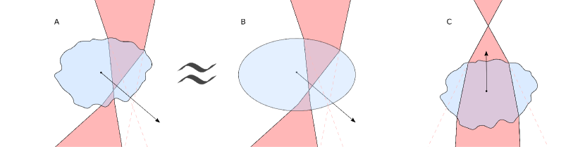
Figure 2: Ray diagrams showing deflection of a beam by a particle. The refractive index of the particle is higher than the refractive index of the background medium. (A) shows a particle with a rough surface, if the surface deviation is small compared to the particle size the situation in (A) is approximately equivalent to a similarly sized spherical particle (B). (C) shows a particle that makes the beam more collimated, the corresponding force experienced by the particle is opposite the beam propagation direction.

2.1.4 Between the Rayleigh and geometric optics regimes

Many of the particles of interest lie between the regimes of applicability of the Rayleigh approximation and geometric optics. Noting that one convenient feature of the geometric optics approximation is the easy visualisation of the fields (i.e., rays), it would be useful to retain this feature in the intermediate regime. For example, we can generate a full-wave equivalent to figure 2, as shown in figure 3.

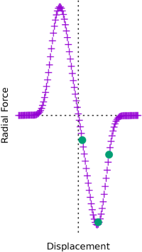
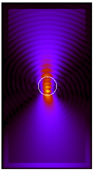
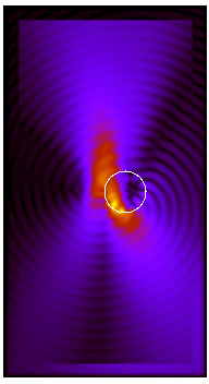
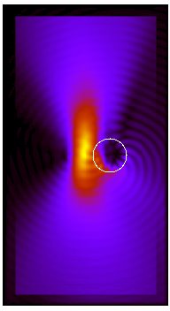
Figure 3: Deflection of a weakly focussed beam by a dielectric particle. The images on the right correspond to the three locations marked on the force-displacement graph.

There are a variety of computational methods that can achieve this. Typically, they involve calculation of the fields over a finite computational volume (which is what lends them so well to visualisation), and the finite extent of this volume can make use of the far-field limit impractical. Thus, the more general procedure described above, using the MST, can be necessary.

3 Finite difference time domain method

The finite difference time domain method is a numerical method for solving systems of partial differential equations that involves storing discrete values for the fields at specific grid locations and repeatedly applying the update equations to advance the fields though time. For optical tweezers simulations, the partial differential equations of interest are the time domain form of the source free Maxwell’s equations,

$$\nabla\times E=-\frac{\partial B}{\partial t}\\$$ (18)

$$\nabla\times H=\frac{\partial D}{\partial t}\\$$ (19)

$$\nabla\cdot D=0\\$$ (20)

$$\nabla\cdot B=0$$ (21)

where $D=\epsilon E$ and $B=\mu H$ are the real valued electric and magnetic vector fields and $\epsilon,\mu$ are the permittivity and permeability values for the field. The discretisation step involves replacing the derivatives with discrete differences, for example

$$\frac{\partial D}{\partial t}\quad\rightarrow\quad\epsilon\frac{E(t+\Delta t/2)-E(t-\Delta t/2)}{\Delta t}\\$$ (22)

$$\left(\nabla\times H\right)_{x}=\frac{\partial H_{z}}{\partial y}-\frac{\partial H_{y}}{\partial z}$$

$$\mkern-40.0mu\quad\rightarrow\quad\frac{H_{z}(y+\Delta y/2)-H_{z}(y-\Delta y/2)}{\Delta y}-\frac{H_{y}(z+\Delta z/2)-H_{y}(z-\Delta z/2)}{\Delta z}$$ (23)

where $\Delta t,\Delta y$ and $\Delta z$ are the time step size and grid spacing along the $y$ and $z$ directions.

For a 1-Dimensional transverse electromagnetic wave propagating along the $z$-axis, with the $E$ field oscillating along the $x$-axis, the corresponding equations are

$$E^{n+1}_{k+1/2}=E^{n}_{k+1/2}-\frac{\Delta t}{\epsilon}\frac{H_{k+1}^{n+1/2}-H_{k}^{n+1/2}}{\Delta z},$$ (24)

$$H^{n+1/2}_{k}=H^{n-1/2}_{k}-\frac{\Delta t}{\mu}\frac{E_{k+1/2}^{n}-E_{k-1/2}^{n}}{\Delta z}.$$ (25)

The subscript refers to the grid location and the superscript refers to the time value. The method achieves second order numerical accuracy by using second order accurate central differences. Rather than store the $E$ and $H$ fields at every grid location, the fields are stored on a staggered grid, as shown in figure 4. For the three dimensional Cartesian case, the arrangement is referred to as the Yee cell. In addition to the grid being spatially staggered, the update equations are also applied at alternate half-integer time steps to achieve second order numerical accuracy for the evolution through time. This approach is sometimes referred to as a leapfrog scheme/method.

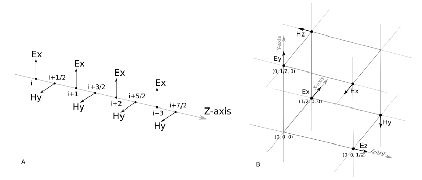
Figure 4: (A) the offset grid used for 1-dimensional FDTD and (B) the Yee cell used for 3-dimensional FDTD.

Optical forces can be calculated from the $E$ and $H$ fields using either the surface or volume integral in (12) and (13). The FDTD method does not calculate all the components of the $E$ and $H$ field at each location. In order to evaluate the MST, the $E$ and $H$ field values surrounding the particle are averaged to produce the necessary components for the $E$ and $H$ fields at the location of interest.

The method requires the fields to be stored at every location throughout the region of interest, such as in and around the particle. At the edges of the simulation space the update equations for the points along the edges depend on terms outside the simulation space. This problem can be resolved in a number of ways: the values outside the simulation space can simply be omitted or the derivatives at the edge set to zero; periodic boundary conditions can be employed where the values from the opposite side of the simulation space are used for the missing values; or absorbing boundary conditions can be used that will absorb any illumination incident on the boundary.

FDTD is of interest for two main reasons: the scalability with problem size and its generality. The method is also convenient if the fields are desired, since the method requires storage of the field values at each grid location. For a spherical particle the number of points and correspondingly the amount of memory required to store the particle scales with the volume $N^{3}$. The total runtime for the simulation depends on the number of points that need to be updated and the time it takes for a wave to propagate across the simulation space which for a spherical particle is proportional to the radius of the particle, so the time scales with $N^{4}$.

The other advantage of FDTD is its generality. The above derivation for the 1-dimensional case assumed an isotropic permittivity, however the method can be extended for anisotropic, conductive and even non-linear materials [16, 17]. The shapes of particles the method can simulate is only dependent on the size and required resolution of the particle features, which in turn depends on the scalability of the method. Multiple types of illumination can be using including plane wave beams and tightly focussed Gaussian beams from pulsed, broadband or continuous sources. For optical tweezers simulations, the main property the method can calculate is optical forces. The method can also be used to calculate various other properties of potential interest to optical tweezers research including torques, internal stresses/strains and absorption/heating.

3.1 Types of illumination

Common types of illumination used for optical tweezers include tightly focussed Gaussian beams, Laguerre–Gaussian beams and evanescent fields at the boundaries of high-low refractive index materials. Situations such as figure 1-A and 1-D can be modelled by describing the incident illumination at one side of the simulation and running the simulation until the fields reach steady state for continuous wave illumination or until the illumination leaves the simulation region for pulsed beams. In some situations it may be necessary to also model parts of the apparatus in order to properly describe the incident illumination or the reflections between the particle and the apparatus. Evanescent fields (figure 1-B/C) can be modelled by introducing the illumination, such as a plane wave or Gaussian beam, onto the interface between high and low refractive index materials at a suitable angle to cause total internal reflection.

A variety of methods exist to introduce illumination sources into FDTD simulations, they fall broadly into two categories: hard sources, which scatter/reflect any fields incident on the source location; and soft sources which allow other fields to pass through the source location. One type of soft source is the total field scattered field (TFSF) which is so named because it separates the simulation space into a region that contains only the scattered fields and a region that contains the total fields (scattered + incident) [17]. In this paper we have used TFSF for introducing sources into our simulations. TFSF allows the incident beam to be introduced on a surface surrounding the particle as long as the values for the $E/H$ fields are known everywhere on the surface. As such, the problem of describing the incident illumination is reduced to a problem of finding an expression for the $E/H$ fields on the surface.

If the $E/H$ field amplitudes are known/computed prior, perhaps as a result of a previous FDTD simulation and stored in a file, the process of introducing the source involves reading in values from the file, interpolating the time/grid coordinates to match the FDTD simulation and adding the fields to the corresponding grid locations. However, many types of beams can be described more simply by their complex field amplitudes or as a decomposition of amplitudes in some basis. For example, a linearly polarized plane wave beam propagating along the $\vec{z}$ direction can be described by the time harmonic complex amplitudes

$$\mathbf{E}=e^{ikz}\vec{x},\qquad\mathbf{H}=\sqrt{\frac{\epsilon}{\mu}}e^{ikz}\vec{y}.$$ (26)

FDTD requires the real field amplitudes, which can be easily calculated from the complex amplitudes

$$E(t)=\Re\left[e^{i\omega t}\mathbf{E}\right],\qquad H(t)=\Re\left[e^{i\omega t}\mathbf{H}\right].$$ (27)

These field values can then be added to the appropriate grid locations at each time step.

As with plane wave beams, Gaussian beams can also be described by a set of complex field amplitudes. A common method involves describing the Gaussian beam in some basis, such as in terms of the vector spherical wave functions, where the $\mathbf{E}$ and $\mathbf{H}$ field amplitudes are given by

$$\mathbf{E}=\sum_{n=1}^{\infty}\sum_{m=-n}^{n}a_{nm}\mathrm{Rg}M_{nm}(kr,\theta,\phi)+b_{nm}\mathrm{Rg}N_{nm}(kr,\theta,\phi)$$ (28)

$$\mathbf{H}=-j\sqrt{\frac{\epsilon}{\mu}}\sum_{n=1}^{\infty}\sum_{m=-n}^{n}b_{nm}\mathrm{Rg}M_{nm}(kr,\theta,\phi)+a_{nm}\mathrm{Rg}N_{nm}(kr,\theta,\phi)$$ (29)

where $(kr,\theta,\phi)$ are the spherical coordinates centred at the beam focus, and $a_{nm},b_{nm}$ are coefficients describing the beam in terms of the regular vector spherical wave functions, VSWFs, $\mathrm{Rg}M_{nm},\mathrm{Rg}N_{nm}$ [16]. A particular beam is then described by a particular set of beam coefficients. Coefficients for Gaussian beams can be calculated for weakly focussed beams using the paraxial approximation and for tightly focussed beams by adding higher order corrections to the paraxial approximation, as is done for the fifth order Davis beam [18, 19] used by [16]. Another approach is to use an over-determined point matching method to determine the beam coefficients [20]. Matlab codes are available as part of the optical tweezers toolbox for computing the beam coefficients for tightly focussed beams including the Laguerre-Gaussian modes with angular momentum [8]. Instead of using a basis of vector spherical wave functions other approaches describe the incident illumination with a plane wave basis. Reference [21] model tightly focussed Hermite-Gaussian beams in FDTD with TFSF using a plane wave basis.

Figure 5 shows plane wave beams, focussed Gaussian beams and Laguerre-Gaussian with different polarisations. The full fields can be visualised in a number of ways including plotting the power density, $E/H$ field components or the $E/H$ field intensity. In this paper we plot the instantaneous $E$ field intensity $|E|^{2}$. For linearly polarized beams this allows the beam wave fronts to be visualised. For circularly polarized beams the field pattern resembles the time averaged field intensity $\langle|E|^{2}\rangle$. When a scattering particle is introduced the reflected light causes interference fringes that can be seen in the $|E|^{2}$ visualisation.

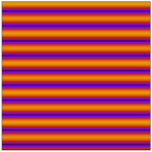
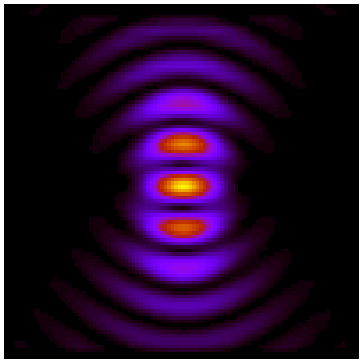
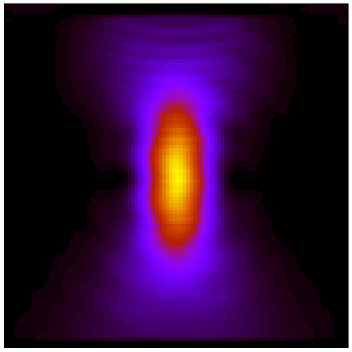
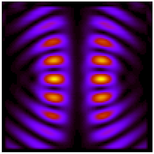
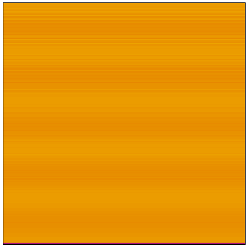
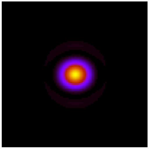
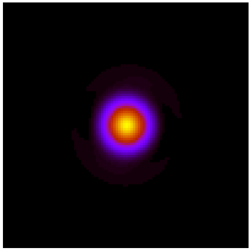
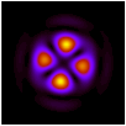
Figure 5: Different types of illumination. Top (left-to-right): Linearly polarized plane wave, linearly polarized focussed Gaussian beam, circularly polarized focussed Gaussian beam, linearly polarized LG02 beam. Bottom: circularly polarized plane wave (left), focal plane images of the beam spot for the above beam types.

4 Simulations

In this section we present the fields and optical forces calculated using the FDTD method for different optical trapping scenarios. The section contains six groups of simulations. Four scenarios involve spherical particles with different sizes and refractive indexes in circular and linearly polarized tightly focussed Gaussian beams. The other two scenarios involve evanescent fields above a high-lower refractive index interface. Calculated forces are normalized by the beam power and speed in medium surrounding the particle to give the dimensionless force efficiencies. The dimensionless force efficiency describes the force in units of $n\hbar k_{0}=\hbar k$ per photon.

Figure 6 shows different sized polystyrene spheres suspended in water illuminated by a circularly polarized focussed Gaussian beam. The numerical aperture (NA) of the beam is 1.02. The illumination wavelength is 800nm in water ($\lambda_{w}$), the refractive index of water and polystyrene are 1.33 and 1.59 respectively. The simulation of the $0.2\lambda_{w}$ particle shows the beam is almost completely unaffected by the presence of the particle. The force the particle experiences is proportional to the gradient of the field amplitude. At the centre of the beam, the gradient is almost zero, and further out the gradient increases in magnitude before falling off quickly as the beam spreads out. For the larger particles the deflection and scattering of the beam is more noticeable; for the $2\lambda_{w}$ axial figure the beam is clearly more focussed.

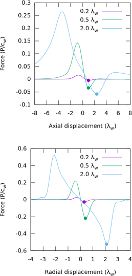
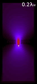
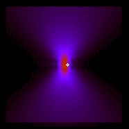
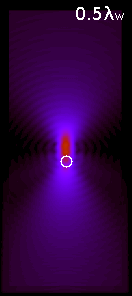
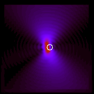
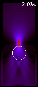
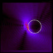
Figure 6: Different sized polystyrene spheres in water.

Figure 7 shows the effect of different refractive indices on the optical force and scattering of the beam by the dielectric sphere. The spheres are illuminated by a linearly polarized Gaussian beam (NA = 1.02), the $E$-field is polarized parallel to the radial displacement direction. The high index (n = 2.0) and very low index (n = 1.2) cases have force-displacement curves that do not correspond to optical trapping. The very low index sphere has a negative force-displacement curve, in the radially displaced field simulation the particle appears to repel the beam, in the axial simulation the beam becomes less collimated. The light that passes through the high index sphere is very collimated, but much more of the light is reflected off the first surface and scattered in other directions.

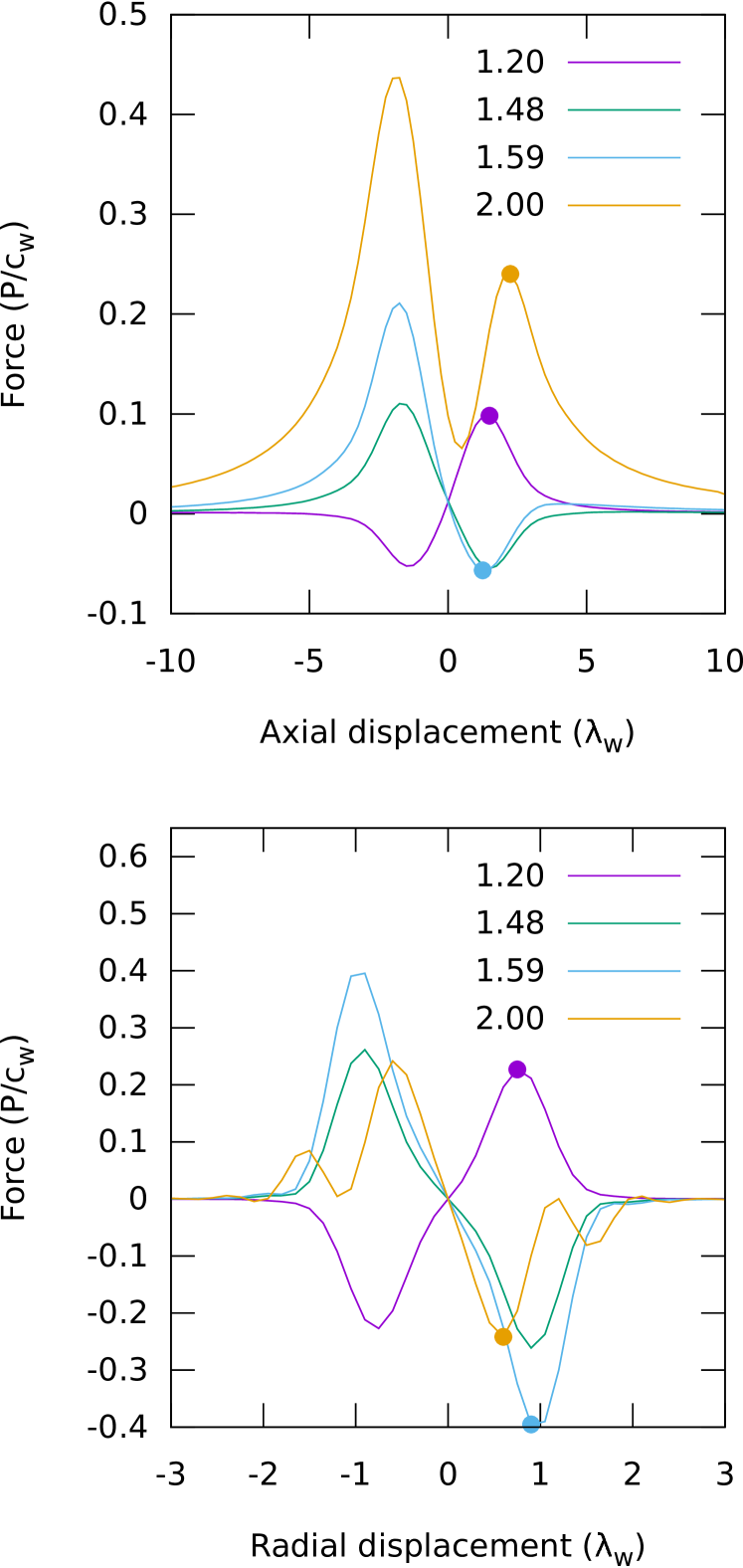
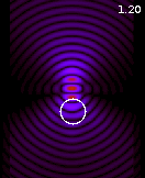
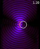
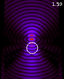
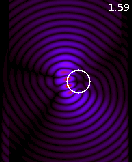
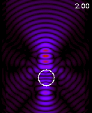
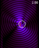
Figure 7: Spheres with different refractive indices suspended in water.

The effect of beam polarisation on the trapping of particles can be important, especially when the surface of the particle is near the edge of the beam. Figure 8 shows the effect of polarisation on the radial force on a high index sphere in water. When the light is incident near normal to the surface, the transmittance between the water and sphere will be almost equal for all polarisation angles. As the incident angle approaches Brewster’s angle, the reflectivity between light polarised perpendicular and parallel to the incident plane becomes noticeably different. In the figure, when the beam is polarised along the Y axis, much more of the light appears to pass into the sphere than in the X case where most of the beam appears to be deflected around the sphere. The fields in the circularly polarized case, with the same total beam power, resemble the sum of the two linear cases; this is also true for the time averaged force.

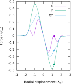
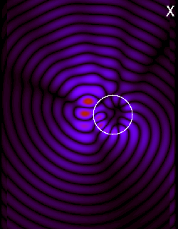
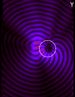
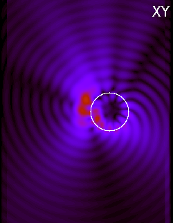
Figure 8: 2$\lambda_{w}$ high index (n = 2.0) sphere in water illuminated by linear and circularly polarised Guassian beams.

The previous figures showed that it is sometimes difficult to trap spheres when there is a high refractive index contrast between the trapping medium and the particle. If it is not possible to change the refractive index of the background medium, one alternative is to coat the particle with an anti-reflective coating. This technique has been demonstrated experimentally for polystyrene spheres coated with silica [22]. Figure 9 shows 4 different types of engineered particles with anti-reflective (AR) coatings surrounding a $1\lambda_{w}$ radius high index (n = 2.0) sphere. The AR coatings form a $1\lambda_{w}$ shell around the sphere. For comparison a $2\lambda_{w}$ high index sphere is also shown.

We thought it would be interesting to try multiple types of AR coatings: two with a single layer of material and two with a graded material. The refractive index of the single layer AR coatings were chosen to be half way between the refractive index of the two materials and half way between the permittivity values of the two materials. The grading was chosen to be linear with respect to the refractive index for one case and linear with respect to the permittivity for the other. The graded AR coatings performed best. For this particular scenario we did not notice any significant difference between the two choices of outer refractive index and the two choices of gradings. This result agrees with the observation by [23] that for single layer coated spheres, improvements to the trapping efficiency are relatively insensitive to refractive index and thickness of the surrounding layer.

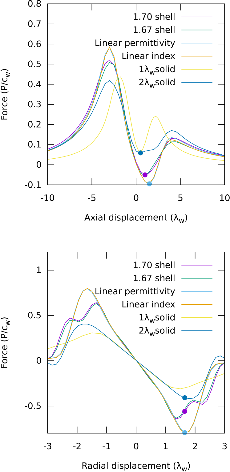
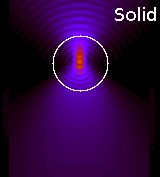
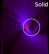
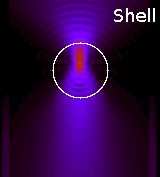
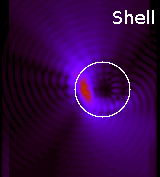
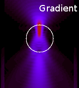
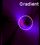
Figure 9: Spherical $1\lambda_{w}$ high index (n = 2.0) sphere coated with different anti-reflective coatings. The Solid case shows a $2\lambda_{w}$ high index sphere for comparison.

The two evanescent field simulations are shown in figure 10 and figure 11. These simulations used an artificial beam located beneath the high-low refractive index interface ($n_{high}=2.0,n_{low}=1.33$). The illuminating beam was a plane wave angled at 43.2 degrees from the surface normal. The calculated forces for the evanescent simulations are all normalized to the maximum force value in figure 10.

Figure 10 involves a single circularly polarized beam. The beam is propagating from right to left. On the far right there are additional non-evanescent fields above the surface, these are an artifact of the beam, similar but smaller artifacts are also present on the far left of the simulation. The evanescent field appears to be coupled into the high index spheres and subsequently be radiated outwards. As a result, the spheres experience a force towards the surface and along the direction of the field. The low index sphere appears to repel the field back down towards the surface, the sphere is repelled from the surface but still pushed along by the field.

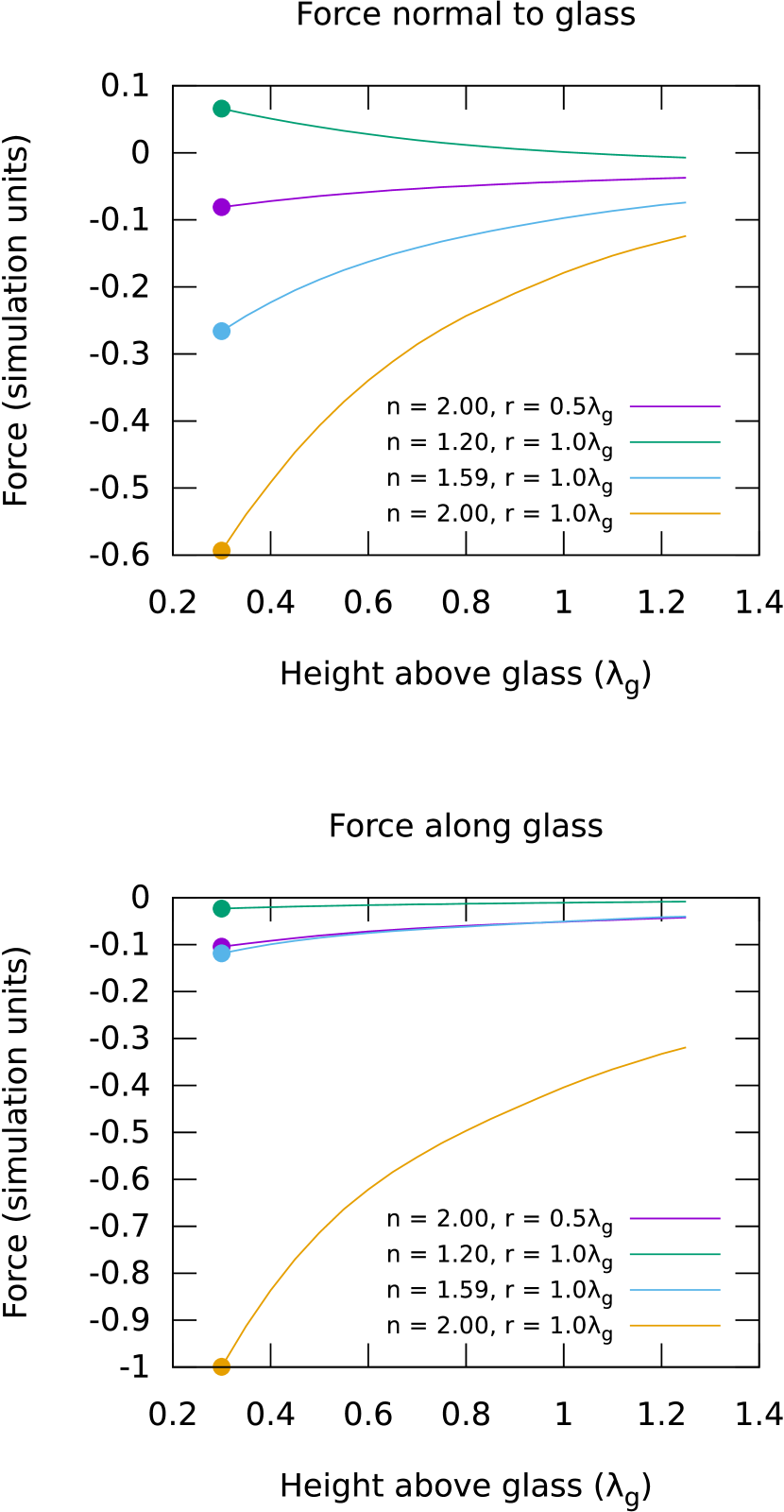
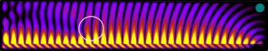
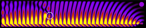
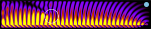
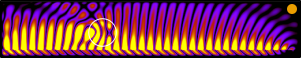
Figure 10: Particles in an evanescent transport beam.

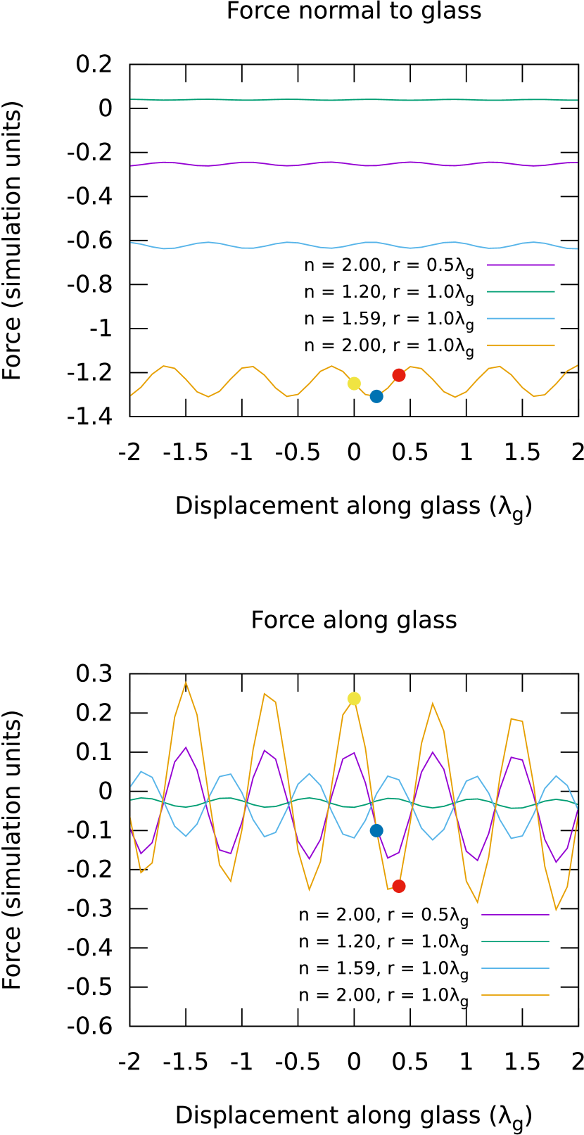
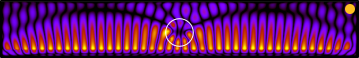
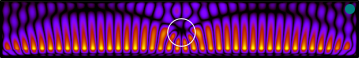
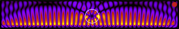
Figure 11: Particles in an evanescent standing wave beam.

Figure 11 involves two linearly polarized illumination sources propagating from opposite ends of the simulation. Similarly to figure 10 the simulation contains artifacts towards the far edges of the simulation due to the type of beam and simulation constraints. Unlike the single beam evanescent field, with multiple beams it is possible to trap and hold a particle in place. Depending on the size and refractive index of the sphere, stable trapping may correspond to the dark spot between evanescent field fringes or the light spot at an evanescent field fringe.

5 Conclusion

In this paper we have discussed optical tweezers, the different regimes for modelling optical tweezers problems and simulations of different scenarios calculated using FDTD. The full field visualisations show the qualitative behaviour of the fields around a scattering particle, providing a similar qualitative insight into the trapping behaviour as the Rayleigh approximation and geometric optics methods with the advantage of providing accurate results in the intermediate regime. Unlike geometric optics, the full field visualisation approach is also able to provide insight into the behaviour of particles in evanescent fields, visually showing the coupling of the field out of the high index material.

FDTD is a useful tool for visualising the fields in and around arbitrary scatterers, the method is very general and can be used for modelling various types of various materials. In this paper we limited our study to particles with spherical symmetry. Particles without rotational symmetry may also experience optical torques from transfer of spin or orbital angular momentum from the beam to the particle. Calculation of optical torques in the near-field using FDTD is difficult. Taking the moment of the force per unit volume using (13) seems like a good starting points, but this approach seems to omit the spin angular momentum. Alternatively, [16] use another stress tensor approach that appears to include the spin in certain circumstances while omitting the orbital angular momentum. It is unclear if a combination of these two approaches can be used to give accurate results. The higher dimensionality also leads to increased difficulty in finding/optimising trapping positions and conditions. For these higher dimensional search spaces an optimisation technique such as simulated annealing might be useful.

The simulations presented in this paper used our new FDTD implementation. Our FDTD implementation is written in C++ utilising newer features of the language including template meta-programming. It is our plan to release the implementation as open source software in the near future.

References

References

- [1] Ashkin A and Dziedzic J M 1971 Applied Physics Letters 19 283–285 URL http://scitation.aip.org/content/aip/journal/apl/19/8/10.1063/1.1653919
- [2] Ashkin A, Dziedzic J M, Bjorkholm J E and Chu S 1986 Opt. Lett. 11 288–290 URL http://ol.osa.org/abstract.cfm?URI=ol-11-5-288
- [3] Tsander F A 1964 Flights to other planets Problems of flight by jet propulsion (Jerusalem: Israel Program for Scientific Translations) pp 221–223 translated from Russian; first published in the Journal “Tekhnike i Zhim”, No. 13, 1924.
- [4] Wang M D, Yin H, Landick R, Gelles J and Block S M 1997 Biophysical journal 72 1335
- [5] Yao A, Tassieri M, Padgett M and Cooper J 2009 Lab Chip 9(17) 2568–2575 URL http://dx.doi.org/10.1039/B907992K
- [6] Nieminen T A, Higuet J, Knöner G G, Loke V L Y, Parkin S, Singer W, Heckenberg N R and Rubinsztein-Dunlop H 2005 Optically driven micromachines: progress and prospects vol 6038 (Proc. SPIE) pp 603813–603813–9 URL http://dx.doi.org/10.1117/12.651760
- [7] Callegari A, Mijalkov M, Gököz A B and Volpe G 2015 J. Opt. Soc. Am. B 32 B11–B19 URL http://josab.osa.org/abstract.cfm?URI=josab-32-5-B11
- [8] Nieminen T A, du Preez-Wilkinson N, Stilgoe A B, Loke V L, Bui A A and Rubinsztein-Dunlop H 2014 Journal of Quantitative Spectroscopy and Radiative Transfer 146 59–80 ISSN 0022-4073 URL http://www.sciencedirect.com/science/article/pii/S0022407314001587
- [9] Fontes A, Neves A A R, Moreira W L, de Thomaz A A, Barbosa L C, Cesar C L and de Paula A M 2005 Applied Physics Letters 87 221109 URL http://dx.doi.org/10.1063/1.2137896
- [10] Rohrbach A 2005 Phys. Rev. Lett. 95(16) 168102 URL http://link.aps.org/doi/10.1103/PhysRevLett.95.168102
- [11] Wriedt T 1998 Particle & Particle Systems Characterization 15 67–74 ISSN 1521-4117 URL http://dx.doi.org/10.1002/(SICI)1521-4117(199804)15:2<67::AID-PPSC67>3.0.CO;2-F
- [12] Nieminen T A, Heckenberg N R and Rubinsztein-Dunlop H 2004 Computational modeling of optical tweezers vol 5514 (Proc. SPIE) pp 514–523 URL http://dx.doi.org/10.1117/12.557090
- [13] Bui A A, Stilgoe A B, Lenton I C, Gibson L J, Kashchuk A V, Zhang S, Rubinsztein-Dunlop H and Nieminen T A 2016 Journal of Quantitative Spectroscopy and Radiative Transfer – ISSN 0022-4073 URL http://www.sciencedirect.com/science/article/pii/S0022407316306422
- [14] Moffitt J R, Chemla Y R, Smith S B and Bustamante C 2008 Annual Review of Biochemistry 77 205–228 pMID: 18307407 URL http://dx.doi.org/10.1146/annurev.biochem.77.043007.090225
- [15] Gordon J P 1973 Physical Review A 8 14–21
- [16] Benito D C, Simpson S H and Hanna S 2008 Opt. Express 16 2942–2957 URL http://www.opticsexpress.org/abstract.cfm?URI=oe-16-5-2942
- [17] Inan U S and Marshall R A 2011 Numerical electromagnetics: the FDTD method (Cambridge;New York;: Cambridge University Press) ISBN 1139011472;9781139011471;
- [18] Barton J P and Alexander D R 1989 Journal of Applied Physics 66 2800–2802 URL http://dx.doi.org/10.1063/1.344207
- [19] Davis L W 1979 Phys. Rev. A 19(3) 1177–1179 URL http://link.aps.org/doi/10.1103/PhysRevA.19.1177
- [20] Nieminen T A, Rubinsztein-Dunlop H and Heckenberg N R 2003 Journal of Quantitative Spectroscopy and Radiative Transfer 79 1005–1017
- [21] İlker R Çapoğlu, Taflove A and Backman V 2013 Opt. Express 21 87–101 URL http://www.opticsexpress.org/abstract.cfm?URI=oe-21-1-87
- [22] Bormuth V, Jannasch A, Ander M, van Kats C M, van Blaaderen A, Howard J and Schäffer E 2008 Opt. Express 16 13831–13844 URL http://www.opticsexpress.org/abstract.cfm?URI=oe-16-18-13831
- [23] Hu Y, Nieminen T A, Heckenberg N R and Rubinsztein-Dunlop H 2008 Journal of Applied Physics 103 093119 URL http://dx.doi.org/10.1063/1.2919574