Two-parameter Asymptotic expansions for elliptic equations with small geometric perturbation and high contrast ratio

Abstract.

We consider the asymptotic solutions of an interface problem corresponding to an elliptic partial differential equation with Dirichlet boundary condition and transmission condition, subject to the small geometric perturbation and the high contrast ratio of the conductivity. We consider two types of perturbations: the first corresponds to a thin layer coating a fixed bounded domain and the second is the perturbation of the interface. As the perturbation size tends to zero and the ratio of the conductivities in two subdomains tends to zero, the two-parameter asymptotic expansions on the fixed reference domain are derived to any order after the single parameter expansions are solved beforehand. Our main tool is the asymptotic analysis based on the Taylor expansions for the properly extended solutions on fixed domains. The Neumann boundary condition and Robin boundary condition arise in two-parameter expansions, depending on the relation of the geometric perturbation size and the contrast ratio.

1. Introduction

Let ${D}\subset\mathbb{R}^{d}$, $d=1,2,3$, be a simply-connected Lipschitz continuous domain. Consider the perturbation of the domain ${D}$ given by the perturbed boundary $\partial{D}_{\varepsilon}$ defined as

$$\partial{D}_{\varepsilon}=\left\{\boldsymbol{x}^{\prime}:\boldsymbol{x}^{\prime}=\boldsymbol{x}+\varepsilon h(\boldsymbol{x})\boldsymbol{n}(\boldsymbol{x}):\boldsymbol{x}\in\partial{D}\right\},$$ (1.1)

where $\varepsilon\in(0,~{}\varepsilon_{0}]$ for a fixed small number $\varepsilon_{0}\ll 1$ represents the small characteristic size of the perturbation, $h(\boldsymbol{x})$ is a continuous function defined on $\partial{D}$, and $\boldsymbol{n}(\boldsymbol{x})$ is the (outward) normal direction of ${D}$. For sufficiently small $\varepsilon$, the boundary $\partial{D}_{\varepsilon}$ uniquely defines a perturbed domain ${D}_{\varepsilon}$. If $h$ is non-negative, then ${D}_{\varepsilon}$ contains ${D}$. We assume that $h$ is a sufficiently smooth function.

The main problem of our concern is related to the following Dirichlet boundary value elliptic problem imposed in the perturbed domain ${D}_{\varepsilon}$:

$$\begin{cases}&\mathcal{L}u_{\varepsilon}=f\quad\text{in }{D}_{\varepsilon},\\ &u_{\varepsilon}=g\quad\text{on }\partial{D}_{\varepsilon},\end{cases}$$ (1.2)

where $\mathcal{L}$ is the second order elliptic operator, having the divergence form

$$\mathcal{L}u=-\sum_{i,j=1}^{d}\partial_{x_{j}}\bigl{(}a^{ij}(\boldsymbol{x})\partial_{x_{i}}u\bigr{)}+\sum_{i=1}^{d}b^{i}(\boldsymbol{x})\partial_{x_{i}}u+c(\boldsymbol{x})u.$$ (1.3)

The second order coefficient functions $a^{ij}$, $i,j=1,\cdots,d$, form a non-degenerate positive definite matrix $\mathsfsl{a}=(a^{ij})$, i.e., $a^{ji}=a^{ij}$, and

$$\sum_{i,j=1}^{d}a^{ij}(\boldsymbol{x})\xi_{i}\xi_{j}>0,$$ (1.4)

for every $\boldsymbol{x}\in\overline{{D}\cup{D}_{\varepsilon_{0}}}$ and non-zero vector $(\xi_{1},\cdots,\xi_{d})\in\mathbb{R}^{d}$. The coefficients $b^{i}$, $i=1,\cdots,d$, and $c$ are assumed smooth in $\mathbb{R}^{d}$. The boundary value function $g$ is also assumed smooth in an open neighbourhood of $\partial{D}$.

If the coefficient $\mathsfsl{a}$ is assumed to be continuous everywhere, then the solution $u_{\varepsilon}$ is the perturbation of a classic elliptic equation with uncertainty in characterizing the domain. How to quantify the uncertainty in the solution due to the geometric perturbation, particularly when $h$ is a random function, is an interesting and important topic in uncertainty quantification. The more challenging case is that $\mathsfsl{a}$ is not continuous across some interface. Then the transmission condition should be specified on the jump interface. In such cases, the interface may also be subject to small perturbations.

There are two scenarios of the geometric perturbations in the transmission problems. The first one is to consider the previous domain perturbation setup with a non-negative $h$, then ${D}\subset{D}_{\varepsilon}$ and the interface is $\Gamma=\partial{D}$, which is fixed and separates the domain ${D}$ and the thin layer

$$L_{\varepsilon}=\left\{\boldsymbol{x}^{\prime}:\boldsymbol{x}^{\prime}=\boldsymbol{x}+th(\boldsymbol{x})\boldsymbol{n}(\boldsymbol{x}),0<t<\varepsilon,\boldsymbol{x}\in\partial{D},h(\boldsymbol{x})\neq 0\right\}.$$

We call this model the thin layer problem. The second scenario is to partition a fixed domain ${D}$ into two subdomains: ${D}={D_{\varepsilon}^{+}}\cup{D_{\varepsilon}^{-}}\cup\Gamma_{\varepsilon},$ where $\Gamma_{\varepsilon}$ is the dividing interface, which is assumed as a perturbation from a fixed interface $\Gamma$. The difference between $\Gamma_{\varepsilon}$ and $\Gamma$ can be also described by a function $h$. The detailed definitions of ${D_{\varepsilon}^{+}},{D_{\varepsilon}^{-}},\Gamma_{\varepsilon}$ will be specified later. We call this model the perturbed interface problem. In the first problem, we attach a thin layer $L_{\varepsilon}$ to encircle the fixed domain ${D}$ and the layer thickness vanishes as $\varepsilon$ tends to zero. The interface there is fixed. In the second problem, we partition a fixed domain ${D}$ into two subdomains ${D}^{\pm}_{\varepsilon}$ by a perturbed interface $\Gamma_{\varepsilon}$ and the two subdomains have comparable size.

All these perturbations can be either deterministic or random, depending on whether $h$ is a deterministic function or a random field. For the latter case, after $h$ is expended in random space by Karhunen-Loève theorem $h(\boldsymbol{x},\omega)=\sum h_{i}(\boldsymbol{x})\phi_{i}(\omega)$, or by the Monte Carlo samples $h(\boldsymbol{x},\omega)\sim h_{i}(\boldsymbol{x})$, the problem usually can be transformed to a set of deterministic perturbations if the correlation length of $h$ is not vanishing. So, we only focus on the deterministic $h$ here; the application to the random case may follow the standard approaches used in many literatures such as [20, 13, 3, 5].

There is a distinctive class of perturbations of the domain for the PDE (1.2): the so called “rough boundary/rough domain”, in which the spatial scale of the profile $h$ also depends on $\varepsilon$, for instance, ${D}$ is perturbed by the form $\varepsilon h_{\varepsilon}(\boldsymbol{x})=\varepsilon\bar{h}(\boldsymbol{x}/\varepsilon)$ for a periodic function $\bar{h}$ (see [15] and references therein). When the boundary condition itself also involves the similar multiscale feature, the multiscale finite element method was applied and analyzed by [17].

To explicitly show the transmission condition and to introduce our second asymptotic parameter other than the perturbation size $\varepsilon$, we take the simplest case of the thin layer problem corresponding to the first scenario mentioned above. In this case, ${D}\subset{D}_{\varepsilon}$, $\Gamma=\partial{D}$ is the interface, separating the domain ${D}$ and the thin layer $L_{\varepsilon}={D}_{\varepsilon}\setminus\bar{{D}}$. Assume that the coefficients $b$ and $c$ vanish and that $\mathsfsl{a}$ is scalar-valued and is piecewisely homogeneous in ${D}$ and $L_{\varepsilon}$. Then the corresponding transmission problem takes the form

$$\begin{cases}&-\Delta u_{\varepsilon}=f\quad\text{in }{{D}},\\ &-\sigma\Delta u_{\varepsilon}=f\quad\text{in }{L_{\varepsilon}},\\ &u_{\mathrm{int}}=u_{\mathrm{ext}},\quad\displaystyle\partial_{\boldsymbol{n}}u_{\mathrm{int}}=\sigma\partial_{\boldsymbol{n}}u_{\mathrm{ext}}\quad\text{on }{\Gamma},\\ &u_{\varepsilon}=0\quad\text{on }\partial{D}_{\varepsilon},\end{cases}$$ (1.5)

where $\sigma$ is a constant parameter representing the ratio of conductivity in two different domains. $u_{\mathrm{int}}$ and $u_{\mathrm{ext}}$ are the restrictions of the solution $u_{\varepsilon}$ on two subdomains $D$ and $L_{\varepsilon}$, respectively. The similar form of the transmission condition will be specified later for the general problems. If the material property across the interface has a significant difference, then the value of $\sigma$ can take a very small value or a very large value. The resulted transmission problem in this high-contrast media is an important subject in multiscale analysis and computation.

The elliptic model (1.2) and the transmission problem such as (1.5) originate from many applications such as diffusion processes, electrostatics, porous media and heat conduction. One of our motivating examples is the diffusion model of exciton in organic semiconductors ([14, 10, 4]). For the discontinuous coefficient model (1.5), a well-known problem is the electromagnetic model for bodies coated with a dielectric layer $L_{\varepsilon}$ with distinctive material coefficients. In porous media applications, the permeability of subsurface regions is described as a quantity with high-contrast and multiscale features.

We here mainly concern the asymptotic analysis in terms of the two different parameters, $\varepsilon$ and $\sigma$, where $\varepsilon$ represents the amplitude of the geometric perturbation on the domain or the interface, and $\sigma$ represents the ratio of different material coefficients. In this paper, we shall first consider the asymptotic effect of each parameter separately and then work on the more complicated two-parameter expansions.

Many theories and methods have been developed and used to study the above elliptic problems and the interface problems. We review some general methodologies on the asymptotic study for the solution $u_{\varepsilon}$ subject to the geometric perturbations. The first idea to handle the irregular domain ${D}_{\varepsilon}$ is the domain mapping, which is to find a smooth mapping to change the irregular domain to a fixed reference domain. See the reference [20, 3, 11] for the applications and the analysis of this method. This method works for any irregular domain as long as a diffeomorphism can be found regardless it is a small perturbation or not. By applying the diffeomorphism transformation, all geometric information is transformed into a new differential operator and a new boundary condition, which are both more complicated than the original form on irregular domain. The second method, particularly for the perturbed interface problem, is a generalization of calculus of variation to the geometric setting — the shape derivative ([12, 13]). The method of shape derivatives is widely used for the sensitivity analysis of the geometry of the boundary and shape optimization. Although it is quite easy to obtain the first few order derivatives, the calculation is very complicated for the higher order derivatives. The last method, which is also our main tool here, is the asymptotic expansion, which actually refers to a collection of problem-specific methods and relies on the correct use of the ansätz ([19, 2, 1, 5]). In this method, by using a good regularity of the solution in the correct (sub)domains, one can apply certain ansätz in the form of the series expansion to approximate the boundary conditions on the fixed domain. More details on the application of this method to our problems of concerns will be reviewed and commented in subsequent sections.

The main motivation of this article is to give a comprehensive study on the (formal) asymptotic expansions of the solutions to the above various elliptic problems, including the thin layer problem and the interface problem, up to an arbitrary order in theory. Specifically, we shall address the following four problems.

1. The first task is that for the elliptic model (1.2) with smooth $\mathsfsl{a}$ , we want to have in ${D}$

   $$u_{\varepsilon}=u_{0}+\varepsilon u_{1}+\varepsilon^{2}u_{2}+\varepsilon^{3}u_{3}+\ldots,$$ (1.6)

   in certain sense, where all terms $u_{i}$ are independent of $\varepsilon$ explicitly. Then we want to construct a sequence $\{u^{[n]}\}$ of functions satisfying the following properties: (i) Each $u^{[n]}$ is the solution to a boundary value problem defined only on the fixed domain ${D}$; (ii) The error between the restriction of $u_{\varepsilon}$ to ${D}$ and $u^{[n]}$ is limited to the order $\mathcal{O}(\varepsilon^{n+1})$; (iii) The numerical computation (which is not our objective in this paper) of $u^{[n]}$ should be easier than directly solving the original equation (1.2). Note that $u^{[n]}$ is not simply the partial sum $\sum_{i=0}^{n}\varepsilon^{n}\,u_{n}$, because the latter may not satisfy a closed boundary value problem.

2. The second task is to generalize the results in (I) to the thin layer problem (1.5) for the case of the discontinuous coefficient $a$.

3. The third one is the generalization of (II) to the high-contrast material, i.e., $\sigma$, the ratio of material coefficients across the interface $\Gamma$, is very large or very small. We want to derive the two-parameter expansions when the limits of both $\varepsilon$ and $\sigma$ are considered. We are concerned with the three scaling regimes for $\varepsilon$ and $\sigma$: $\varepsilon/\sigma\rightarrow 0$, $\varepsilon/\sigma\rightarrow\infty$, and $\varepsilon/\sigma\rightarrow c\in(0,~{}\infty)$. The final result is the boundary value problem for each term in the two-parameter asymptotic expansions $u_{\mathrm{int}}(\boldsymbol{x})=\sum_{m,n}u_{m,n}(\boldsymbol{x})\varepsilon^{m}\mu^{n}$, where $m,n$ are integers, and $\mu$ is linked to the ratio of $\varepsilon$ and $\mu$, whose specific form depends on the asymptotic regimes. We shall show that the three scalings will give arise to the Dirichlet, Neumann or Robbin boundary condition for $u_{m,n}$, respectively.

4. The last one is on the perturbed interface problem where the interface $\Gamma_{\varepsilon}$ is not fixed as in (II) and (III), but is associated with a perturbed domain partition ${D}={D_{\varepsilon}^{+}}\cup{D_{\varepsilon}^{-}}\cup\Gamma_{\varepsilon}$. Meanwhile, the high-contrast ratio limit is also considered, and we derive the two-parameter asymptotic expansions, where we find there is no special dependence on the scaling of $\varepsilon$ and $\sigma$.

From Section 2 to Section 5, we solve each of these four problems in each section. The techniques we used for (I) and (II) are different from the existing methods. The two-parameter asymptotic expansions for (III) and (IV) in this paper are new results. The main techniques we apply here for all four problems are the Taylor expansion applied in various contents, which all requires a good regularity of the underlying function. For the thin layer problem or the interface problem, where the solution $u_{\varepsilon}$ apparently does not posses such smoothness on the interface, our idea is first to extend each smooth component of the solution $u_{\varepsilon}$ on each subdomain onto some $\varepsilon$-independent domains before applying any asymptotic expansions. This is achieved by imposing certain Cauchy problems on the interface when interpreting the elliptic equation as a time-evolution equation in which the normal direction of the interface is the time marching direction. The second important idea is to apply the inverse Lax-Wendroff procedure ([18]) to convert the high order derivatives in the normal direction on the interface to those along the tangent directions and the first order normal derivative, for which the original transmission condition on the interface is utilized.

To end this introduction, we review several existing works which are closely related to the problems we considered here. The work in [5] considered the thin layer problem (1.5) with a fixed $\sigma$ as $\varepsilon\to 0$. The main idea in [5] is to write the differential operator $\mathcal{L}$ in terms of local coordinate in the thin layer $L_{\varepsilon}$, and apply the ansätz $\mathcal{L}=\sum_{n\geqslant-2}\varepsilon^{n}\mathcal{L}_{n}$ to derive a system of (infinitely number of) recursive equations for the expansion of the solution in this dilated layer. Then with the aid of the transmission condition on the interface $\Gamma$, the boundary conditions of these equations in the layer $L_{\varepsilon}$ are linked to the solutions in the interior (fixed) domain ${D}$. In [1], to assist the construction of local solutions in the multiscale finite element methods for the elliptic equations in high-contrast media, the authors derived asymptotic expansions for the solutions of the elliptic problems with high contrast ratio, i.e., $\sigma$ tends to $0$ or $\infty$. But their analysis is for the fixed domain and interface.

2. The elliptic problem with smooth coefficients

In this section, we study the equation (1.2) on ${D}_{\varepsilon}$ by assuming that $\mathsfsl{a}(\boldsymbol{x})$ is sufficiently smooth everywhere and $h(\boldsymbol{x})$ in (1.1) is also sufficiently smooth on $\partial{D}$. This means that the Taylor expansion for these two functions are available up to any order. The signs of $h(\boldsymbol{x})$ can be arbitrary at different $\boldsymbol{x}\in\partial{D}$ and the operator $\mathcal{L}$ in (1.3) is not limited to the Laplace operator.

Recall that the perturbed thin layer $L_{\varepsilon}$ is defined by

$$L_{\varepsilon}=\left\{\boldsymbol{x}^{\prime}:\boldsymbol{x}^{\prime}=\boldsymbol{x}+th(\boldsymbol{x})\boldsymbol{n}(\boldsymbol{x}),0<t<\varepsilon,\boldsymbol{x}\in\partial{D},h(\boldsymbol{x})\neq 0\right\}.$$

The condition $h(\boldsymbol{x})\neq 0$ ensures that $L_{\varepsilon}$ is also a domain (open set). Depending on the sign of the function $h$, we can decompose the thin layer $L_{\varepsilon}$ into the interior layer $L_{\varepsilon,\mathrm{int}}$ and the external layer $L_{\varepsilon,\mathrm{ext}}$:

$$L_{\varepsilon}=L_{\varepsilon,\mathrm{int}}\cup L_{\varepsilon,\mathrm{ext}},$$

where

$$L_{\varepsilon,\mathrm{int}}:=L_{\varepsilon}\cap{D}=\left\{\boldsymbol{x}^{\prime}:\boldsymbol{x}^{\prime}=\boldsymbol{x}+th(\boldsymbol{x})\boldsymbol{n}(\boldsymbol{x}),0<t<\varepsilon,\boldsymbol{x}\in\partial{D},h(\boldsymbol{x})<0\right\},$$

$$L_{\varepsilon,\mathrm{ext}}:=L_{\varepsilon}\setminus{D}=\left\{\boldsymbol{x}^{\prime}:\boldsymbol{x}^{\prime}=\boldsymbol{x}+th(\boldsymbol{x})\boldsymbol{n}(\boldsymbol{x}),0<t<\varepsilon,\boldsymbol{x}\in\partial{D},h(\boldsymbol{x})>0\right\}.$$

$L_{\varepsilon,\mathrm{int}}\subset{D}$ and $L_{\varepsilon,\mathrm{ext}}\cap{D}=\emptyset$. Then ${D}_{\varepsilon}$ is the interior of $\overline{({D}\setminus L_{\varepsilon,\mathrm{int}})\cup L_{\varepsilon,\mathrm{ext}}}.$ Refer to the schematic illustration in Figure 1.

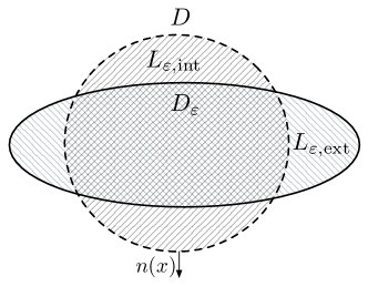
Figure 1. Schematic illustration of the domain perturbation. The regular domain ${D}$ is in the “ball” shape and the perturbed domain ${D}_{\varepsilon}$ is in the “ellipse” shape.

2.1. Approximate expansions

The problem (1.2) is defined on the $\varepsilon$-dependent domain ${D}_{\varepsilon}$. We extend it to a fixed domain ${D}\cup{D}_{\varepsilon_{0}}$ and justify this extension in Section 2.1.1. Then in Section 2.1.2, we use the Taylor expansion near $\partial{D}$ to derive the asymptotic expansion $u_{\varepsilon}=\sum_{n\geqslant 0}\varepsilon^{n}u_{n}$, for which the inverse Lax-Wendroff procedure is applied to convert the high order normal derivatives into the first order normal derivative and the tangential derivatives along the boundary $\partial{D}$.

[5] already derived the first three terms, $u_{0}$, $u_{1}$ and $u_{2}$. But the method we give below seems simpler and does not require the dilation technique and any asymptotic form for the differential operator $\mathcal{L}$ used in [5]. Actually, that kind of singular perturbation suits for the case that the solution itself develops a sharp peak in the thin layer, such as the traditional boundary layer analysis in fluid mechanics. However, the problem here does not have this feature and the solutions on ${D}$ and ${D}_{\varepsilon}$ both behave very normally at the order $\mathcal{O}(1)$. We find that the direct expansion for the boundary condition of $u_{\varepsilon}$ in an appropriate way is sufficient to derive the boundary condition of $u_{n}$. To present our main technique, we start with the smooth $\mathsfsl{a}$ case in this section and then show how to generalize to the discontinuous $\mathsfsl{a}$ in Section 3.

2.1.1. The extension of the solution to the fixed domain

Note that ${D}\cup{D}_{\varepsilon}$ is increasing in $\varepsilon$ since $L_{\varepsilon,\mathrm{ext}}$ always expands as $\varepsilon$ increases. So it is convenient to make the extension to the whole domain ${D}\cup{D}_{\varepsilon_{0}}$ since we only consider $\varepsilon\in(0,~{}\varepsilon_{0}]$. On this fixed domain ${D}\cup{D}_{\varepsilon_{0}}$, the solution is known on the part $\overline{{D}_{\varepsilon}}$; we thus consider the difference $\triangle_{\varepsilon}$ which consists of the disjoint thin layers:

$$\triangle_{\varepsilon}:=({D}\cup{D}_{\varepsilon_{0}})\setminus\overline{{D}_{\varepsilon}}=L_{\varepsilon,\mathrm{int}}\cup N_{\varepsilon},~{}~{}\mbox{ where }N_{\varepsilon}:=L_{\varepsilon_{0},\mathrm{ext}}\setminus\overline{L_{\varepsilon,\mathrm{ext}}}.$$

Denote the solution extended on $\triangle_{\varepsilon}$ by $\tilde{u}_{\varepsilon}$, and assume that $\tilde{u}_{\varepsilon}$ and $u_{\varepsilon}$ have the same values and the same normal derivatives on the common boundary $\partial{D}_{\varepsilon}$. Specifically, $\tilde{u}_{\varepsilon}$ is the unique solution to the following Cauchy problem posed in the thin layers $L_{\varepsilon,\mathrm{int}}$ and $N_{\varepsilon}$:

$$\begin{cases}\mathcal{L}\tilde{u}_{\varepsilon}=f\qquad&\text{in }L_{\varepsilon,\mathrm{int}}\cup N_{\varepsilon},\\ \tilde{u}_{\varepsilon}=u_{\varepsilon}=g,\quad\partial_{\boldsymbol{n}}\tilde{u}_{\varepsilon}=\partial_{\boldsymbol{n}}u_{\varepsilon}\quad&\text{on }\partial{D}_{\varepsilon},\end{cases}$$ (2.1)

where $u_{\varepsilon}$, the solution to equation (1.2), is presumably given, $\boldsymbol{n}$ is the outward normal of ${D}_{\varepsilon}$ on $\partial{D}_{\varepsilon}$. Note that $\partial{D}_{\varepsilon}$ is a proper subset of the boundaries of $L_{\varepsilon,\mathrm{int}}$ and $N_{\varepsilon}$. The problem (2.1) is actually a Cauchy problem of $\tilde{u}_{\varepsilon}$, not a boundary-valued elliptic problem, because the value and the “velocity” of $\tilde{u}_{\varepsilon}$ are specified on $\partial{D}_{\varepsilon}$ — a part of its complete boundary. The boundary $\partial{D}_{\varepsilon}$ satisfies the noncharacteristic condition $\sum_{i,j=1}^{d}a^{ij}n_{i}n_{j}\neq 0$ trivially since $\mathcal{L}$ is, by assumption, an elliptic operator satisfying (1.4). Thus by the Cauchy-Kovalevskaya theorem ([7]), the solution on $\partial{D}$ can propagate to the boundary $\partial\triangle_{\varepsilon}$ and the above Cauchy problem (2.1) is well-posed for sufficiently small $\varepsilon_{0}$.

Remark 2.1.

The above method of extending the solution to a larger (and $\varepsilon$-indepedent) domain can also preserve the regularity of the solution and helps clarify the rigorous meaning of the Taylor expansion we shall apply. This extension idea by the use of the Cauchy problem of a time-evolution equation will be applied repeatedly in this paper, especially for the interface problem so that each smooth component of the solution on each subdomain may be approximated by the Taylor expansion along some interface.

Now it is clear that we can define a function $w_{\varepsilon}$ piecewisely on the whole (fixed) domain $\overline{{D}}\cup\overline{{D}_{\varepsilon_{0}}}=\overline{{D}_{\varepsilon}}\cup\overline{\triangle_{\varepsilon}}$ as follows:

$$w_{\varepsilon}(\boldsymbol{x}):=\begin{cases}u_{\varepsilon}(\boldsymbol{x})&\mbox{ in }\overline{{D}_{\varepsilon}},\\ \tilde{u}_{\varepsilon}(\boldsymbol{x})&\mbox{ in }\overline{\triangle_{\varepsilon}}.\end{cases}$$ (2.2)

This definition is justified by the boundary condition in (2.1) which dictates that $u_{\varepsilon}$ and $\tilde{u}_{\varepsilon}$ coincide on the common boundary $\partial{D}_{\varepsilon}$. Then $w_{\varepsilon}$ satisfies the equation on the fixed domain

$$\mathcal{L}w_{\varepsilon}=f\quad\text{in }{D}\cup{D}_{\varepsilon_{0}},$$ (2.3)

and on the $\varepsilon$-dependent boundary.

$$w_{\varepsilon}=g,\quad\text{on }\partial{D}_{\varepsilon}.$$ (2.4)

Note that (2.4) does not serve as a boundary condition to the equation (2.3). $w_{\varepsilon}$ is simply a combination of $u_{\varepsilon}$ from the boundary value problem (1.2) and $\tilde{u}_{\varepsilon}$ from the Cauchy problem (2.1) . The above argument of extension ensures that $w_{\varepsilon}$ has the same regularity of $u_{\varepsilon}$, but on ${D}\cup{D}_{\varepsilon_{0}}$.

2.1.2. Asymptotic expansion on the whole domain

By the above extension, we can assume the following ansätz for $w_{\varepsilon}$,

$$w_{\varepsilon}(\boldsymbol{x})=\sum_{n=0}^{\infty}\varepsilon^{n}w_{n}(\boldsymbol{x})\quad\text{for }\boldsymbol{x}\in\overline{{D}\cup{D}_{\varepsilon_{0}}}.$$ (2.5)

Plug this ansätz into the equation (2.3), and match the terms at the same order of $\varepsilon$, then we obtain the following equations for $w_{n}$ in ${D}\cup{D}_{\varepsilon_{0}}$:

$$\mathcal{L}w_{n}=\delta_{0,n}f.$$ (2.6)

Here $\delta_{i,j}=1$ if $i=j$ and $\delta_{i,j}=0$ if $i\neq j$.

For the condition (2.4), $w_{\varepsilon}=g$ on $\partial{D}_{\varepsilon}$, by noticing the fact that $\boldsymbol{x}+\varepsilon h(\boldsymbol{x})\boldsymbol{n}(\boldsymbol{x})\in\partial{D}_{\varepsilon}$ for all $\boldsymbol{x}\in\partial{D}$, we have

$$w_{\varepsilon}\bigl{(}\boldsymbol{x}+\varepsilon h(\boldsymbol{x})\boldsymbol{n}(\boldsymbol{x})\bigr{)}=\sum_{n=0}^{\infty}\varepsilon^{n}w_{n}\bigl{(}\boldsymbol{x}+\varepsilon h(\boldsymbol{x})\boldsymbol{n}(\boldsymbol{x})\bigr{)}=g\bigl{(}\boldsymbol{x}+\varepsilon h(\boldsymbol{x})\boldsymbol{n}(\boldsymbol{x})\bigr{)}.$$ (2.7)

The Taylor expansions in $\varepsilon$ on the right-hand side read

$$w_{n}\bigl{(}\boldsymbol{x}+\varepsilon h(\boldsymbol{x})\boldsymbol{n}(\boldsymbol{x})\bigr{)}=\sum_{k=0}^{\infty}\frac{\varepsilon^{k}\bigl{(}h(\boldsymbol{x})\bigr{)}^{k}}{k!}{\partial_{\boldsymbol{n}}^{k}}w_{n}(\boldsymbol{x}),$$ (2.8)

$$g(\boldsymbol{x}+\varepsilon h(\boldsymbol{x})\boldsymbol{n}(\boldsymbol{x}))=\sum_{k=0}^{\infty}\frac{\varepsilon^{k}\bigl{(}h(\boldsymbol{x})\bigr{)}^{k}}{k!}{\partial_{\boldsymbol{n}}^{k}}g(\boldsymbol{x}),$$ (2.9)

where for any vector field $\boldsymbol{n}(\boldsymbol{x})=\bigl{(}n_{1}(\boldsymbol{x}),\cdots,n_{d}(\boldsymbol{x})\bigr{)}$, the $k$-th directional derivative along $\boldsymbol{n}$ at $\boldsymbol{x}=\boldsymbol{x}_{0}$ is defined by

$$\partial_{\boldsymbol{n}}^{k}\big{|}_{\boldsymbol{x}=\boldsymbol{x}_{0}}:=\biggr{(}\sum_{i=1}^{d}n_{i}(\boldsymbol{x}_{0})\partial_{x_{i}}\bigg{|}_{\boldsymbol{x}=\boldsymbol{x}_{0}}\biggr{)}^{k}.$$

Then (2.7), (2.8) and (2.9) together lead to

$$\sum_{n=0}^{\infty}\varepsilon^{n}\sum_{k=0}^{\infty}\frac{\varepsilon^{k}\bigl{(}h(\boldsymbol{x})\bigr{)}^{k}}{k!}{\partial_{\boldsymbol{n}}^{k}}w_{n}(\boldsymbol{x})=\sum_{k=0}^{\infty}\frac{\varepsilon^{k}\bigl{(}h(\boldsymbol{x})\bigr{)}^{k}}{k!}{\partial_{\boldsymbol{n}}^{k}}g(\boldsymbol{x}),$$

which, by a change of the indices $m=k+n$, is equivalent to

$$\sum_{m=0}^{\infty}\varepsilon^{m}\sum_{k=0}^{m}\frac{\bigl{(}h(\boldsymbol{x})\bigr{)}^{k}}{k!}{\partial_{\boldsymbol{n}}^{k}}w_{m-k}(\boldsymbol{x})=\sum_{m=0}^{\infty}\frac{\varepsilon^{m}\bigl{(}h(\boldsymbol{x})\bigr{)}^{m}}{m!}{\partial_{\boldsymbol{n}}^{m}}g(\boldsymbol{x}).$$

Then by matching the terms with the same order of $\varepsilon$, we obtain that

$$\sum_{k=0}^{m}\frac{\bigl{(}h(\boldsymbol{x})\bigr{)}^{k}}{k!}{\partial_{\boldsymbol{n}}^{k}}w_{m-k}(\boldsymbol{x})=\frac{\bigl{(}h(\boldsymbol{x})\bigr{)}^{m}}{m!}{\partial_{\boldsymbol{n}}^{m}}g(\boldsymbol{x}),$$

i.e.,

$$\begin{cases}w_{0}(\boldsymbol{x})=g(\boldsymbol{x}),\\ w_{m}(\boldsymbol{x})=\dfrac{\bigl{(}h(\boldsymbol{x})\bigr{)}^{m}}{m!}{\partial_{\boldsymbol{n}}^{m}}g(\boldsymbol{x})-\displaystyle\sum_{k=1}^{m}\dfrac{\bigl{(}h(\boldsymbol{x})\bigr{)}^{k}}{k!}{\partial_{\boldsymbol{n}}^{k}}w_{m-k}(\boldsymbol{x}),~{}~{}\forall m\geqslant 1.\end{cases}$$ (2.10)

This provides a recursive expression of the boundary condition on $\partial{D}$ for the $m$-th order term $w_{m}$.

Define $u_{n}$ as the restriction of $w_{n}$ to ${D}$. Then $u_{\varepsilon}=\sum_{n=0}^{\infty}\varepsilon^{n}u_{n}$. By (2.6) and (2.10), $u_{n}$ satisfies the following sequence of boundary value problems on ${D}$ where the boundary conditions on $\partial{D}$ are defined recursively:

$$\begin{cases}&\mathcal{L}u_{0}=f\quad\text{in }{D},\\ &u_{0}=g\quad\text{on }\partial{D},\end{cases}$$ (2.11)

and for $n\geqslant 1$,

$$\begin{cases}&\mathcal{L}u_{n}=0\quad\text{in }{D},\\ &u_{n}(\boldsymbol{x})=\dfrac{\bigl{(}h(\boldsymbol{x})\bigr{)}^{n}}{n!}{\partial_{\boldsymbol{n}}^{n}}g(\boldsymbol{x})-\displaystyle\sum_{k=1}^{n}\dfrac{\bigl{(}h(\boldsymbol{x})\bigr{)}^{k}}{k!}{\partial_{\boldsymbol{n}}^{k}}u_{n-k}(\boldsymbol{x})\quad\text{on }\partial{D}.\end{cases}$$ (2.12)

In particular, for $n=1,2,3$, the above boundary conditions on $\partial{D}$ are

$$u_{1}(\boldsymbol{x})=h(\boldsymbol{x})\partial_{\boldsymbol{n}}g(\boldsymbol{x})-h(\boldsymbol{x})\partial_{\boldsymbol{n}}u_{0}(\boldsymbol{x}),$$ (2.13)

$$u_{2}(\boldsymbol{x})=\dfrac{\bigl{(}h(\boldsymbol{x})\bigr{)}^{2}}{2}{\partial_{\boldsymbol{n}}^{2}}g(\boldsymbol{x})-h(\boldsymbol{x})\partial_{\boldsymbol{n}}u_{1}(\boldsymbol{x})-\dfrac{\bigl{(}h(\boldsymbol{x})\bigr{)}^{2}}{2}{\partial_{\boldsymbol{n}}^{2}}u_{0}(\boldsymbol{x}),$$ (2.14)

$$u_{3}(\boldsymbol{x})=\dfrac{\bigl{(}h(\boldsymbol{x})\bigr{)}^{3}}{6}\partial_{\boldsymbol{n}}^{3}g(\boldsymbol{x})-h(\boldsymbol{x})\partial_{\boldsymbol{n}}u_{2}(\boldsymbol{x})-\dfrac{\bigl{(}h(\boldsymbol{x})\bigr{)}^{2}}{2}\partial_{\boldsymbol{n}}^{2}u_{1}(\boldsymbol{x})-\dfrac{\bigl{(}h(\boldsymbol{x})\bigr{)}^{3}}{6}\partial_{\boldsymbol{n}}^{3}u_{0}(\boldsymbol{x}).$$ (2.15)

Remark 2.2.

Using the shape calculus method, one may also derive a “shape-Taylor expansion” of $u_{\varepsilon}$ on any compact set $K\subset{D}\cap{D}_{\varepsilon}$ (see [12] and the references therein),

$$u_{\varepsilon}(\boldsymbol{x})=u_{0}(\boldsymbol{x})+\varepsilon\mathrm{d}[\boldsymbol{U}](\boldsymbol{x})+\frac{\varepsilon^{2}}{2}\mathrm{d}^{2}[\boldsymbol{U},\boldsymbol{U}](\boldsymbol{x})+\mathcal{O}(\varepsilon^{3}),$$

where $u_{0}$ is the solution to (2.11), $\mathrm{d}[\boldsymbol{U}]$ is the first order shape derivative on the boundary variation $\boldsymbol{U}$, which is given by the Dirichlet problem

$$\begin{cases}&\mathcal{L}\mathrm{d}[\boldsymbol{U}]=0\quad\text{in }{D},\\ &\mathrm{d}[\boldsymbol{U}]=\boldsymbol{U}\cdot\boldsymbol{n}\partial_{\boldsymbol{n}}(g-u_{0})\quad\text{on }\partial{D}.\end{cases}$$

$\mathrm{d}^{2}[\boldsymbol{U},\boldsymbol{U}^{\prime}]$ is the second order shape derivative, i.e., the “shape Hessian”, on the pair $(\boldsymbol{U},\boldsymbol{U}^{\prime})$ of boundary variations, which is given by the Dirichlet problem

$$\begin{cases}&\mathcal{L}\mathrm{d}^{2}[\boldsymbol{U},\boldsymbol{U}^{\prime}]=0\quad\text{in }{D},\\ &\mathrm{d}^{2}[\boldsymbol{U},\boldsymbol{U}^{\prime}]=\partial_{\boldsymbol{U}}\partial_{\boldsymbol{U}^{\prime}}(g-u_{0})-\partial_{\boldsymbol{U}}\mathrm{d}[\boldsymbol{U}^{\prime}]-\partial_{\boldsymbol{U}^{\prime}}\mathrm{d}[\boldsymbol{U}]\quad\text{on }\partial{D}.\end{cases}$$

It is easy to see that when the boundary variation $\boldsymbol{U}(\boldsymbol{x})$ is given by $\boldsymbol{U}(\boldsymbol{x})=h(\boldsymbol{x})\boldsymbol{n}(\boldsymbol{x})$ for $\boldsymbol{x}\in\partial{D}$, then $\mathrm{d}[\boldsymbol{U}]=u_{1}$ and $\mathrm{d}^{2}[\boldsymbol{U},\boldsymbol{U}]=2u_{2}$. Therefore the shape calculus method produces the same result as our method.

The right-hand side of the boundary condition (2.12) for each $u_{n}$ involves the normal derivatives of all lower order terms. The inverse Lax-Wendroff procedure, which is used to construct high order numerical methods such as in [18], enables us to convert the high order normal derivatives into the first order normal derivative and the tangential derivatives on the boundary $\partial{D}$. See Lemma 2.3 below. This conversion procedure here seems only optional in theory, but as we shall show in Section 3, for piecewisely smooth coefficients, this step is essential for the use of transmission conditions on the interface to link the interior solution and the exterior solution.

Lemma 2.3.

Let $u$ satisfy $\mathcal{L}u=f$ where $\mathcal{L}$ is the elliptic operator in (1.3). Then all the normal derivatives $\partial_{\boldsymbol{n}}^{k}u$ on a smooth surface $\Gamma$ with order $k\geqslant 2$ can be expressed in terms of the boundary $\Gamma$, the restrictions of the function $u$ and its normal derivative $\partial_{\boldsymbol{n}}u$ on $\Gamma$, and the coefficient functions $a^{ij}$, $b^{i}$, $c$, $i,j=1,\cdots,d$. Therefore for every $k\geqslant 2$, every smooth surface $\Gamma$, every elliptic operator $\mathcal{L}$ and every smooth function $f$, there exists an operator

$$F_{k,\Gamma,\mathcal{L},f}[\cdot,\cdot]$$

acting on a pair of functions defined on $\Gamma$ such that for any smooth function $u$ satisfying $\mathcal{L}u=f$, its $k$-th normal derivative $\partial_{\boldsymbol{n}}^{k}u$ on $\Gamma$ is given by $F_{k,\Gamma,\mathcal{L},f}[u,\partial_{\boldsymbol{n}}u]$.

In addition, it is easy to see the following properties of the operator $F_{k,\Gamma,\mathcal{L},f}[\cdot,\cdot]$ from the linearity of $\mathcal{L}$:

$$F_{k,\Gamma,\mathcal{L},f}[u,\partial_{\boldsymbol{n}}u]+F_{k,\Gamma,\mathcal{L},\varphi}[v,\partial_{\boldsymbol{n}}v]=F_{k,\Gamma,\mathcal{L},f+\varphi}[u+v,\partial_{\boldsymbol{n}}u+\partial_{\boldsymbol{n}}v],$$

$$cF_{k,\Gamma,\mathcal{L},f}[u,\partial_{\boldsymbol{n}}u]=F_{k,\Gamma,\mathcal{L},cf}[cu,c\partial_{\boldsymbol{n}}u],\quad\forall c\in\mathbb{R},$$

where $u$ and $v$ solve $\mathcal{L}u=f$ and $\mathcal{L}v=\varphi$ respectively. In particular, taking $c=0$ in the last equality yields $F_{k,\Gamma,\mathcal{L},0}[0,0]=0$.

For the proof of this lemma, refer to Theorem 1 in Section 4.6 of [7]. The crucial assumption for the proof is the noncharacteristic condition of $\Gamma$, which is automatically guaranteed by the ellipticity of $\mathcal{L}$. This lemma will be used later multiple times and the dependency on $\Gamma$ and $\mathcal{L}$ in the notation of the mapping $F$ may be dropped out if they are self-explanatory.

With this notation $F$, the boundary condition for $u_{n}(n\geqslant 1)$ in (2.12) can be formally written as

$$\begin{split}u_{n}(\boldsymbol{x})=~{}~{}&\dfrac{\bigl{(}h(\boldsymbol{x})\bigr{)}^{n}}{n!}{\partial_{\boldsymbol{n}}^{n}}g(\boldsymbol{x})-h(\boldsymbol{x})\partial_{\boldsymbol{n}}u_{n-1}(\boldsymbol{x})\\ &-\displaystyle\sum_{k=2}^{n}\dfrac{\bigl{(}h(\boldsymbol{x})\bigr{)}^{k}}{k!}F_{k,\partial{D},\mathcal{L},\delta_{k,n}f}[u_{n-k},\partial_{\boldsymbol{n}}u_{n-k}](\boldsymbol{x}).\end{split}$$

To demonstrate the above theory and show how the conversion of the higher order normal derivatives works, in Appendix A, we present two examples in 2D. The first is our motivating example of exciton diffusion and the second is the Poisson equation. Furthermore, in Appendix A, we demonstrate how to generalize our method to the Neumann boundary condition and the reaction-diffusion equation with nonlinear terms.

2.2. The partial sums

We have formally derived the hierarchic systems of the boundary value problems for the expansion terms $\left\{u_{n}\right\}$ in Section 2.1. We next derive the closed boundary value problems which the partial sums approximately satisfy. The procedure is the same as in [5]. Define the partial sums

$$v^{[n]}(\boldsymbol{x}):=\sum_{k=0}^{n}\varepsilon^{k}u_{k}(\boldsymbol{x}),\quad n\geqslant 0.$$

On the boundary $\partial{D}$, by using (2.12), we have

$$\begin{split}v^{[n]}(\boldsymbol{x})&=\sum_{k=0}^{n}\varepsilon^{k}u_{k}(\boldsymbol{x})\\ &=\sum_{k=0}^{n}\frac{\varepsilon^{k}\bigl{(}h(\boldsymbol{x})\bigr{)}^{k}}{k!}{\partial_{\boldsymbol{n}}^{k}}g(\boldsymbol{x})-\sum_{k=0}^{n}\varepsilon^{k}\sum_{j=1}^{k}\dfrac{\bigl{(}h(\boldsymbol{x})\bigr{)}^{j}}{j!}{\partial_{\boldsymbol{n}}^{j}}u_{k-j}(\boldsymbol{x})\\ &=\sum_{k=0}^{n}\frac{\varepsilon^{k}\bigl{(}h(\boldsymbol{x})\bigr{)}^{k}}{k!}{\partial_{\boldsymbol{n}}^{k}}g(\boldsymbol{x})-\sum_{j=1}^{n}\dfrac{\varepsilon^{j}{\bigl{(}h(\boldsymbol{x})\bigr{)}^{j}}}{j!}{\partial_{\boldsymbol{n}}^{j}}v^{[n-j]}(\boldsymbol{x}).\end{split}$$ (2.16)

It is worth pointing out that the system of the boundary value problems for $v^{[n]}$ is defined recursively. To obtain $v^{[n]}$, one needs to solve the boundary value problems from $v^{[0]}$ (i.e., $u_{0}$) up to $v^{[n-1]}$. Thus, in total, $(n+1)$ Dirichlet boundary value problems have to be solved. However, it is possible to directly solve one boundary value problem to obtain the approximation with the same order as $v^{[n]}$ by replacing the $v^{[n-j]}$ terms on the right-hand side of (2.16) by $v^{[n]}$. Then one obtains the following closed boundary value problem, whose solution is denoted by $u^{[n]}$:

$$\begin{cases}&\mathcal{L}u^{[n]}=f\quad\text{in }{D},\\ &\displaystyle\sum_{k=0}^{n}\dfrac{\varepsilon^{k}\bigl{(}h(\boldsymbol{x})\bigr{)}^{k}}{k!}{\partial_{\boldsymbol{n}}^{k}}u^{[n]}(\boldsymbol{x})=\sum_{k=0}^{n}\frac{\varepsilon^{k}\bigl{(}h(\boldsymbol{x})\bigr{)}^{k}}{k!}{\partial_{\boldsymbol{n}}^{k}}g(\boldsymbol{x})\quad\text{on }\partial{D}.\end{cases}$$ (2.17)

In particular, the boundary value problems for $u^{[1]}$ and $u^{[2]}$ are

$$\begin{cases}&\mathcal{L}u^{[1]}=f\quad\text{in }{D},\\ &u^{[1]}+\varepsilon h\partial_{\boldsymbol{n}}u^{[1]}=g+\varepsilon h\partial_{\boldsymbol{n}}g\quad\text{on }\partial{D},\end{cases}$$

$$\begin{cases}&\mathcal{L}u^{[2]}=f\quad\text{in }{D},\\ &u^{[2]}+\varepsilon h\partial_{\boldsymbol{n}}u^{[2]}+\dfrac{\varepsilon^{2}h^{2}}{2}{\partial_{\boldsymbol{n}}^{2}}u^{[2]}=g+\varepsilon h\partial_{\boldsymbol{n}}g+\dfrac{\varepsilon^{2}h^{2}}{2}{\partial_{\boldsymbol{n}}^{2}}g\quad\text{on }\partial{D}.\end{cases}$$

The following theorem gives the approximation error of $v^{[n]}$, whose proof is given in Appendix B.1.

Assumption 2.4.

Assume ${D}\subset{D}_{\varepsilon}\subset{D}_{\varepsilon_{0}}$ and $\partial{D}\in C^{\infty}$. Let the operator $\mathcal{L}$ given by (1.3) be strictly elliptic in ${D}_{\varepsilon_{0}}$ and have the coefficients $a^{ij}$, $b^{i}$, $c$ belong to $C^{\infty}(\overline{{D}_{\varepsilon_{0}}})$ and $c\geqslant 0$. Also assume $f,g\in C^{\infty}(\overline{{D}_{\varepsilon_{0}}})$ and $h\in C^{\infty}(\partial{D})$.

Theorem 2.5.

Under the Assumption 2.4, $\forall n,m\geqslant 0$,

$$\bigl{\|}v^{[n]}-u_{\varepsilon}\bigr{\|}_{H^{m}({D})}=\mathcal{O}(\varepsilon^{n+1}).$$ (2.18)

The following approximation error of $u^{[n]}$ has been proved in [5] for $n=0,1,2$,

$$\bigl{\|}u^{[n]}-u_{\varepsilon}\bigr{\|}_{H^{1}({D})}=\mathcal{O}(\varepsilon^{n+1}).$$

Note that although $u^{[n]}$ and $v^{[n]}$ have the same approximation order, there might still be a considerable difference in the accuracy of their approximation errors due to the effects of the prefactors. The numerical results in [5] show that the approximation $u^{[n]}$ produces much less accurate results than $v^{[n]}$ for $n=1,2$. This can be easily confirmed by the following simple one-dimensional example:

$$\begin{cases}&u_{\varepsilon}^{\prime\prime}=2\quad\text{in }{D}_{\varepsilon}=(0,~{}1+\varepsilon),\\ &u_{\varepsilon}(0)=u_{\varepsilon}(1+\varepsilon)=0.\end{cases}$$

The true solution is $u_{\varepsilon}(x)=x^{2}-(1+\varepsilon)x$. The equation for $u_{0}$ reads

$$\begin{cases}&u_{0}^{\prime\prime}=2\quad\text{in }{D}=(0,~{}1),\\ &u_{0}(0)=u_{0}(1)=0,\end{cases}$$

with the solution $u_{0}(x)=x^{2}-x$. Then the equation for $u_{1}$ is

$$\begin{cases}&u_{1}^{\prime\prime}=0\quad\text{in }{D}=(0,~{}1),\\ &u_{1}(0)=0,\quad u_{1}(1)=-u_{0}^{\prime}(1)=-1.\end{cases}$$

So $u_{1}(x)=-x$, and then the partial sum $v^{[1]}(x)=u_{0}(x)+\varepsilon u_{1}(x)=x^{2}-x-\varepsilon x$. Hence

$$v^{[1]}(x)-u_{\varepsilon}(x)=0.$$

The equation for $u^{[1]}$ is

$$\begin{cases}&\bigl{(}u^{[1]}\bigr{)}^{\prime\prime}=2\quad\text{in }{D}=(0,~{}1),\\ &u^{[1]}(0)=0,\quad u^{[1]}(1)+\varepsilon\bigl{(}u^{[1]}\bigr{)}^{\prime}(1)=0.\end{cases}$$

We find $u^{[1]}(x)=x^{2}-\dfrac{1+2\varepsilon}{1+\varepsilon}x$, which is a worse approximation than $v^{[1]}$ since

$$u^{[1]}(x)-u_{\varepsilon}(x)=\dfrac{\varepsilon^{2}}{1+\varepsilon}x=\mathcal{O}(\varepsilon^{2}).$$

To attain the zero error as $v^{[1]}$, one needs to proceed to the next order $u^{[2]}$ by solving

$$\begin{cases}&\bigl{(}u^{[2]}\bigr{)}^{\prime\prime}=2\quad\text{in }{D}=(0,~{}1),\\ &u^{[2]}(0)=0,\quad u^{[2]}(1)+\varepsilon\bigl{(}u^{[2]}\bigr{)}^{\prime}(1)+\varepsilon^{2}=0.\end{cases}$$

It turns out $u^{[2]}(x)=v^{[1]}(x)=x^{2}-x-\varepsilon x$.

3. The thin layer problem

Next, we generalize the above method from the continuous material coefficients $\mathsfsl{a}(\boldsymbol{x})$ to the transmission problem associated with the piecewisely smooth coefficients. The Taylor expansion used in Section 2.1 is still applicable since we essentially apply the expansion on each subdomain where $\mathsfsl{a}$ is smooth. The next step is to use Lemma 2.3 (the inverse Lax-Wendroff procedure) to convert the high order normal derivatives on the interface to the first order normal derivative and the tangential derivatives. This critical step facilitates the transmission condition given on the interface to build the connection between the solutions on each subdomain.

For ease of exposition, we only deal with the outward perturbation where $h(\boldsymbol{x})\geqslant 0$ for all $\boldsymbol{x}\in\partial{D}$. So ${D}$ is a (proper) subset of ${D}_{\varepsilon}$ and the difference ${D}_{\varepsilon}\setminus\overline{{D}}$ is the thin layer $L_{\varepsilon}$. The transmission condition is thus imposed on

$$\Gamma:=\left\{\boldsymbol{x}\in\partial{D}:h(\boldsymbol{x})>0\right\}\subset\partial{D}.$$

Note that $\overline{\Gamma}=\partial{D}\cap\partial L_{\varepsilon}$ and $\partial{D}\setminus\Gamma=\left\{\boldsymbol{x}\in\partial{D}:h(\boldsymbol{x})=0\right\}=\partial{D}\cap\partial{D}_{\varepsilon}$. Assume that the second order coefficients $a^{ij}$, $i,j=1,\cdots,d$, are piecewisely smooth and have jumps only across the transmission interface $\Gamma$. In addition, the term $f$ on the right-hand side of the equation is also allowed (but not necessarily) to have jumps on $\Gamma$. Specifically, we assume for $i,j=1,\cdots,d$,

$$a^{ij}(\boldsymbol{x})=\begin{cases}&a^{ij}_{\mathrm{int}}(\boldsymbol{x})\quad\text{for }\boldsymbol{x}\in{{D}}\\ &a^{ij}_{\mathrm{ext}}(\boldsymbol{x})\quad\text{for }\boldsymbol{x}\in L_{\varepsilon_{0}}\end{cases},\quad f(\boldsymbol{x})=\begin{cases}&f_{\mathrm{int}}(\boldsymbol{x})\quad\text{for }\boldsymbol{x}\in{{D}}\\ &f_{\mathrm{ext}}(\boldsymbol{x})\quad\text{for }\boldsymbol{x}\in L_{\varepsilon_{0}}\end{cases},$$

where $a^{ij}_{\mathrm{int}}$ and $f_{\mathrm{int}}$ are smooth functions on $\overline{{D}}$ while $a^{ij}_{\mathrm{ext}}$ and $f_{\mathrm{ext}}$ smooth on $\overline{L_{\varepsilon_{0}}}$, and in general, $a^{ij}_{\mathrm{int}}(\boldsymbol{x})\neq a^{ij}_{\mathrm{ext}}(\boldsymbol{x})$ for $\boldsymbol{x}\in\Gamma$.

Write

$$u(\boldsymbol{x})=\begin{cases}&u_{\mathrm{int}}(\boldsymbol{x})\quad\text{for }\boldsymbol{x}\in{{D}},\\ &u_{\mathrm{ext}}(\boldsymbol{x})\quad\text{for }\boldsymbol{x}\in L_{\varepsilon},\end{cases}$$

then the transmission problem of our concern takes the form:

$$\begin{cases}&\mathcal{L}u_{\mathrm{int}}=f_{\mathrm{int}}\quad\text{in }{{D}},\\ &\mathcal{L}u_{\mathrm{ext}}=f_{\mathrm{ext}}\quad\text{in }{L_{\varepsilon}},\\ &u_{\mathrm{int}}=u_{\mathrm{ext}},\quad\displaystyle\sum_{i,j=1}^{d}a^{ij}_{\mathrm{int}}n_{i}\partial_{x_{j}}u_{\mathrm{int}}=\sum_{i,j=1}^{d}a^{ij}_{\mathrm{ext}}n_{i}\partial_{x_{j}}u_{\mathrm{ext}}\quad\text{on }{\Gamma},\\ &u_{\mathrm{int}}=g\quad\text{on }{\partial{D}_{\varepsilon}\cap\partial{D}},\\ &u_{\mathrm{ext}}=g\quad\text{on }{\partial{D}_{\varepsilon}}\cap\partial L_{\varepsilon}.\end{cases}$$ (3.1)

3.1. Asymptotic expansions in ${D}$ and $L_{\varepsilon}$

Conceptually, we may first extend the domain of $u_{\mathrm{ext}}$ to a fixed larger domain $L_{\varepsilon_{0}}$, as in Section 2.1.1, and for simplicity we still use $u_{\mathrm{ext}}$ for its extension. Assume the following two ansätze for $u_{\mathrm{int}}$ and $u_{\mathrm{ext}}$ respectively:

$$u_{\mathrm{int}}(\boldsymbol{x})=\displaystyle\sum_{n=0}^{\infty}\varepsilon^{n}u_{\mathrm{int},n}(\boldsymbol{x})\quad\text{for }\boldsymbol{x}\in{D},$$ (3.2)

$$u_{\mathrm{ext}}(\boldsymbol{x})=\displaystyle\sum_{n=0}^{\infty}\varepsilon^{n}u_{\mathrm{ext},n}(\boldsymbol{x})\quad\text{for }\boldsymbol{x}\in L_{\varepsilon_{0}}.$$ (3.3)

Plug these ansätze into (3.1), and match the terms at the same order of $\varepsilon$, then we obtain the following equations for $u_{\mathrm{int},n}$ and $u_{\mathrm{ext},n}$,

$$\mathcal{L}u_{\mathrm{int},n}=\delta_{0,n}f_{\mathrm{int}}~{}~{}\text{in }{D},~{}~{}\mbox{ and }~{}\mathcal{L}u_{\mathrm{ext},n}=\delta_{0,n}f_{\mathrm{ext}}~{}~{}\text{in }L_{\varepsilon_{0}},$$

and the transmission conditions on $\Gamma$ for $u_{\mathrm{int},n}$ and $u_{\mathrm{ext},n}$,

$$u_{\mathrm{int},n}=u_{\mathrm{ext},n},$$ (3.4)

$$\sum_{i,j=1}^{d}a^{ij}_{\mathrm{int}}n_{i}\partial_{x_{j}}u_{\mathrm{int},n}=\sum_{i,j=1}^{d}a^{ij}_{\mathrm{ext}}n_{i}\partial_{x_{j}}u_{\mathrm{ext},n}.$$ (3.5)

The boundary conditions on $\partial{D}_{\varepsilon}\cap\partial{D}$ for $u_{\mathrm{int},n}$ is $u_{\mathrm{int},n}=\delta_{0,n}g$ and $u_{\mathrm{ext},n}$ share the same condition on $\partial{D}_{\varepsilon}\cap\partial L_{\varepsilon}$.

Our goal is to derive the correct boundary conditions on $\partial{D}$ for $u_{\mathrm{int},n}$. Note that we already have these conditions on $\partial{D}\cap\partial{D}_{\varepsilon}$, thus it remains to find the boundary conditions on $\Gamma$ for $u_{\mathrm{int},n}$. To this end, we actually first derive the boundary conditions on $\Gamma$ for $u_{\mathrm{ext},n}$, and then convert $u_{\mathrm{ext},n}$ to $u_{\mathrm{int},n}$ by the transmission conditions (3.4) and (3.5).

To work on the exterior solution $u_{\mathrm{ext}}$, which behaves nicely in $L_{\varepsilon_{0}}$, we apply the Taylor expansion method used in Section 2.1.2 to the ansätz (3.3) with the boundary condition $u_{\mathrm{ext}}=g$ on $\partial{D}_{\varepsilon}\cap\partial L_{\varepsilon}$. The obtained result is the following recursive expression of the boundary conditions on $\Gamma$ for $u_{\mathrm{ext},n}$:

$$\begin{cases}u_{\mathrm{ext},0}=g,\\ \begin{split}u_{\mathrm{ext},n}&=\dfrac{h^{n}}{n!}{\partial_{\boldsymbol{n}}^{n}}g-\displaystyle\sum_{k=1}^{n}\dfrac{h^{k}}{k!}{\partial_{\boldsymbol{n}}^{k}}u_{\mathrm{ext},n-k}\\ &=\dfrac{h^{n}}{n!}{\partial_{\boldsymbol{n}}^{n}}g-h\partial_{\boldsymbol{n}}u_{\mathrm{ext},n-1}\\ &~{}~{}~{}\qquad-\sum_{k=2}^{n}\dfrac{h^{k}}{k!}F_{k,\delta_{k,n}f_{\mathrm{ext}}}[u_{\mathrm{ext},n-k},\partial_{\boldsymbol{n}}u_{\mathrm{ext},n-k}],~{}~{}~{}\forall n\geqslant 1,\end{split}\end{cases}$$ (3.6)

where the operator $F_{k,f}$ is the operator $F_{k,\Gamma,\mathcal{L},f}$ introduced in Lemma 2.3 and the subindices $\Gamma$ and $\mathcal{L}$ are dropped for simplicity.

To handle the terms $\partial_{\boldsymbol{n}}u_{\mathrm{ext},n-k}$ on the right-hand side of (3.6), we need the following lemma, proven in Appendix B.2.

Lemma 3.1.

For any integer $n\geqslant 0$ and any $\boldsymbol{x}\in\Gamma$, one can uniquely determine the value of the normal derivative $\partial_{\boldsymbol{n}}u_{\mathrm{ext},n}(\boldsymbol{x})$ on $\Gamma$ from the information of $u_{\mathrm{int},n}$ by using (3.4) and (3.5). More precisely, $\partial_{\boldsymbol{n}}u_{\mathrm{ext},n}(\boldsymbol{x})$ for $\boldsymbol{x}\in\Gamma$ only depends on

• the normal vector $\boldsymbol{n}=\boldsymbol{n}(\boldsymbol{x})$ and

• the value of $u_{\mathrm{int},n}(\boldsymbol{x}^{\prime})$for all $\boldsymbol{x}^{\prime}\in\Gamma$ and

• $\partial_{\boldsymbol{n}}u_{\mathrm{int},n}(\boldsymbol{x})$ and

• the second order coefficients $a^{ij}_{\mathrm{int}}(\boldsymbol{x})$ and $a^{ij}_{\mathrm{ext}}(\boldsymbol{x})$, $i,j=1,\cdots,d$.

Now the transmission conditions (3.4) and (3.5), serve the bridge from $u_{\mathrm{ext},n}$ to $u_{\mathrm{int},n}$, with the aid of Lemma 3.1. Then the calculation following the procedure in the proof of Lemma 3.1 shows that (3.6) leads to the following final results for the boundary condition of $\left\{u_{\mathrm{int},n}\right\}$ on $\Gamma$:

$$\begin{cases}u_{\mathrm{int},0}=g,\\ \begin{split}u_{\mathrm{int},n}&=\dfrac{h^{n}}{n!}{\partial_{\boldsymbol{n}}^{n}}g-hq_{1}-\sum_{k=2}^{n}\dfrac{h^{k}}{k!}F_{k,\delta_{k,n}f_{\mathrm{ext}}}\left[u_{\mathrm{int},n-k},q_{k}\right],\forall n\geqslant 1,\end{split}\end{cases}$$ (3.7)

where for any $\boldsymbol{x}\in\partial{D}$,

$$q_{k}(\boldsymbol{x}):=\frac{Q_{\mathrm{int}}(\boldsymbol{n})\partial_{\boldsymbol{n}}u_{\mathrm{int},n-k}+\sum_{i,j=1}^{d}(a^{ij}_{\mathrm{int}}-a^{ij}_{\mathrm{ext}})n_{i}\partial_{\boldsymbol{\tau}_{j}}u_{\mathrm{int},n-k}}{Q_{\mathrm{ext}}(\boldsymbol{n})},$$

$$Q_{\mathrm{ext}}(\boldsymbol{n}):=\sum_{i,j=1}^{d}a^{ij}_{\mathrm{ext}}n_{i}n_{j},\quad Q_{\mathrm{int}}(\boldsymbol{n}):=\sum_{i,j=1}^{d}a^{ij}_{\mathrm{int}}n_{i}n_{j},$$

Remark 3.2.

Since we have $h=0$ and $u_{\mathrm{int},n}=\delta_{0,n}g$ on the boundary $\partial{D}\setminus\Gamma$, the boundary conditions (3.7) also holds on $\partial{D}\setminus\Gamma$ and thus on the whole boundary $\partial{D}$.

As an illuminating example, let us consider the elliptic operator $\mathcal{L}=-\nabla\cdot\bigl{(}\sigma(\boldsymbol{x})\nabla\bigr{)}$ with a discontinuous $\sigma(\boldsymbol{x})$, which has been studied in Example A.2 when $\sigma(\boldsymbol{x})$ is a smooth function.

Example 3.3.

Set $g=0$ and $\mathcal{L}=-\nabla\cdot\bigl{(}\sigma(\boldsymbol{x})\nabla\bigr{)}$. Assume

$$\sigma(\boldsymbol{x})=\begin{cases}&\sigma_{\mathrm{int}}(\boldsymbol{x})\quad\text{for }\boldsymbol{x}\in{{D}},\\ &\sigma_{\mathrm{ext}}(\boldsymbol{x})\quad\text{for }\boldsymbol{x}\in L_{\varepsilon_{0}},\end{cases}$$ (3.8)

where $\sigma_{\mathrm{int}}$ and $\sigma_{\mathrm{ext}}$ are smooth functions on $\overline{{D}}$ and $\overline{L_{\varepsilon_{0}}}$ respectively, and in general, they are distinct on the common boundary. To ensure the ellipticity of $\mathcal{L}$, we assume that $\sigma_{\mathrm{int}}$ and $\sigma_{\mathrm{ext}}$ are both positive everywhere in their domain. Then the transmission condition (3.5) reads

$$\sigma_{\mathrm{int}}\partial_{\boldsymbol{n}}u_{\mathrm{int},n}=\sigma_{\mathrm{ext}}\partial_{\boldsymbol{n}}u_{\mathrm{ext},n}.$$

Thus we deduce

$$\partial_{\boldsymbol{n}}u_{\mathrm{ext},n}=\frac{\sigma_{\mathrm{int}}\partial_{\boldsymbol{n}}u_{\mathrm{int},n}}{\sigma_{\mathrm{ext}}}.$$ (3.9)

Next, we compute explicitly the boundary conditions on $\Gamma$ for the first three orders $u_{\mathrm{int},n}$.

Order $n=0$. The boundary condition (3.7) on $\Gamma$ for $u_{\mathrm{int},0}$ is simply

$$u_{\mathrm{int},0}=0.$$ (3.10)

Order $n=1$. The boundary condition (3.6) on $\Gamma$ for $u_{\mathrm{ext},1}$ reads

$$u_{\mathrm{ext},1}(\boldsymbol{x})=-h(\boldsymbol{x}){\partial_{\boldsymbol{n}}}u_{\mathrm{ext},0}(\boldsymbol{x}).$$

Then by (3.4) and (3.9), we obtain the boundary condition on $\Gamma$ for $u_{\mathrm{int},1}$:

$$u_{\mathrm{int},1}=-\frac{h\sigma_{\mathrm{int}}}{\sigma_{\mathrm{ext}}}{\partial_{\boldsymbol{n}}}u_{\mathrm{int},0}.$$ (3.11)

Order $n=2$. Applying the boundary condition (A.8) for $u_{2}$ in Example A.2 to $u_{\mathrm{ext},2}$ yields

$$u_{\mathrm{ext},2}=-h\partial_{\boldsymbol{n}}u_{\mathrm{ext},1}+\frac{h^{2}}{2}\Bigl{(}\frac{\partial_{\boldsymbol{n}}\sigma_{\mathrm{ext}}}{\sigma_{\mathrm{ext}}}+\kappa\Bigr{)}\partial_{\boldsymbol{n}}u_{\mathrm{ext},0}+\dfrac{h^{2}f_{\mathrm{ext}}}{2\sigma_{\mathrm{ext}}}.$$

$\kappa$ is the curvature of $\partial{D}$, defined in Example A.2. Then substituting (3.4) and (3.9) into the last equation gives the boundary condition on $\Gamma$ for $u_{\mathrm{int},2}$:

$$u_{\mathrm{int},2}=-\frac{h\sigma_{\mathrm{int}}}{\sigma_{\mathrm{ext}}}{\partial_{\boldsymbol{n}}}u_{\mathrm{int},1}+\frac{h^{2}\sigma_{\mathrm{int}}}{2\sigma_{\mathrm{ext}}}\Bigl{(}\frac{\partial_{\boldsymbol{n}}\sigma_{\mathrm{ext}}}{\sigma_{\mathrm{ext}}}+\kappa\Bigr{)}\partial_{\boldsymbol{n}}u_{\mathrm{int},0}+\dfrac{h^{2}f_{\mathrm{ext}}}{2\sigma_{\mathrm{ext}}}.$$ (3.12)

3.2. The approximate boundary conditions for the partial sums

Define the partial sums

$$v^{[n]}(\boldsymbol{x})=\begin{cases}&v^{[n]}_{\mathrm{int}}(\boldsymbol{x}):=\displaystyle\sum_{k=0}^{n}\varepsilon^{k}u_{\mathrm{int},k}(\boldsymbol{x})\quad\text{for }\boldsymbol{x}\in{D},\\ &v^{[n]}_{\mathrm{ext}}(\boldsymbol{x}):=\displaystyle\sum_{k=0}^{n}\varepsilon^{k}u_{\mathrm{ext},k}(\boldsymbol{x})\quad\text{for }\boldsymbol{x}\in L_{\varepsilon_{0}}.\\ \end{cases}$$

As in Section 2.2, the goal here is to derive the recursive boundary condition for the partial sums and to find the closed boundary value problems for the approximations $u^{[n]}$.

To derive the boundary conditions that the partial sums $v^{[n]}_{\mathrm{int}}$ satisfy, we have two equivalent approaches. The first one is to directly derive the boundary conditions for $v^{[n]}_{\mathrm{int}}$ from the boundary conditions for $u_{\mathrm{int},n}$ which are already obtained above; the second approach is to apply (2.16) to $v^{[n]}_{\mathrm{ext}}$ and then transfer to $v^{[n]}_{\mathrm{int}}$ via the following transmission conditions

$$v^{[n]}_{\mathrm{int}}=v^{[n]}_{\mathrm{ext}},$$

$$\sum_{i,j=1}^{d}a^{ij}_{\mathrm{int}}n_{i}\partial_{x_{j}}v^{[n]}_{\mathrm{int}}=\sum_{i,j=1}^{d}a^{ij}_{\mathrm{ext}}n_{i}\partial_{x_{j}}v^{[n]}_{\mathrm{ext}},$$

which can be easily deduced from (3.4) and (3.5). Let us continue to work on Example 3.3 to illustrate the first approach.

Order $n=1$. On the boundary $\partial{D}$, (3.10) and (3.11) give

$$v^{[1]}_{\mathrm{int}}=-\varepsilon\frac{h\sigma_{\mathrm{int}}}{\sigma_{\mathrm{ext}}}{\partial_{\boldsymbol{n}}}u_{\mathrm{int},0}=-\frac{\varepsilon h\sigma_{\mathrm{int}}}{\sigma_{\mathrm{ext}}}{\partial_{\boldsymbol{n}}}v_{\mathrm{int}}^{[0]}.$$ (3.13)

Then we are motivated to introduce the following Robin boundary value problem for $u^{[1]}$:

$$\begin{cases}&\mathcal{L}u^{[1]}=f\quad\text{in }{D},\\ &u^{[1]}+\dfrac{\varepsilon h\sigma_{\mathrm{int}}}{\sigma_{\mathrm{ext}}}{\partial_{\boldsymbol{n}}}u^{[1]}=0\quad\text{on }\partial{D}.\end{cases}$$ (3.14)

Order $n=2$. On the boundary $\partial{D}$, (3.12) and (3.13) show

$$\begin{split}v^{[2]}_{\mathrm{int}}&=-\frac{\varepsilon h\sigma_{\mathrm{int}}}{\sigma_{\mathrm{ext}}}{\partial_{\boldsymbol{n}}}v_{\mathrm{int}}^{[0]}-\frac{\varepsilon^{2}h\sigma_{\mathrm{int}}}{\sigma_{\mathrm{ext}}}{\partial_{\boldsymbol{n}}}u_{\mathrm{int},1}+\frac{\varepsilon^{2}h^{2}\sigma_{\mathrm{int}}}{2\sigma_{\mathrm{ext}}}\Bigl{(}\frac{\partial_{\boldsymbol{n}}\sigma_{\mathrm{ext}}}{\sigma_{\mathrm{ext}}}+\kappa\Bigr{)}\partial_{\boldsymbol{n}}u_{\mathrm{int},0}+\dfrac{\varepsilon^{2}h^{2}f_{\mathrm{ext}}}{2\sigma_{\mathrm{ext}}}\\ &=-\frac{\varepsilon h\sigma_{\mathrm{int}}}{\sigma_{\mathrm{ext}}}{\partial_{\boldsymbol{n}}}v_{\mathrm{int}}^{[1]}+\frac{\varepsilon^{2}h^{2}\sigma_{\mathrm{int}}}{2\sigma_{\mathrm{ext}}}\Bigl{(}\frac{\partial_{\boldsymbol{n}}\sigma_{\mathrm{ext}}}{\sigma_{\mathrm{ext}}}+\kappa\Bigr{)}\partial_{\boldsymbol{n}}v^{[0]}_{\mathrm{int}}+\dfrac{\varepsilon^{2}h^{2}f_{\mathrm{ext}}}{2\sigma_{\mathrm{ext}}},\end{split}$$

thus the closed Robin boundary value problem for $u^{[2]}$ can be imposed as:

$$\begin{cases}&\mathcal{L}u^{[2]}=f\quad\text{in }{D},\\ &u^{[2]}+\dfrac{\varepsilon h\sigma_{\mathrm{int}}}{\sigma_{\mathrm{ext}}}{\partial_{\boldsymbol{n}}}u^{[2]}-\dfrac{\varepsilon^{2}h^{2}\sigma_{\mathrm{int}}}{2\sigma_{\mathrm{ext}}}\Bigl{(}\dfrac{\partial_{\boldsymbol{n}}\sigma_{\mathrm{ext}}}{\sigma_{\mathrm{ext}}}+\kappa\Bigr{)}\partial_{\boldsymbol{n}}u^{[2]}=\dfrac{\varepsilon^{2}h^{2}f_{\mathrm{ext}}}{2\sigma_{\mathrm{ext}}}\quad\text{on }\partial{D}.\end{cases}$$ (3.15)

To compare with the results derived in [5] where the coefficient $\sigma$ is piecewise constant, we set $\sigma_{\mathrm{int}}=\sigma_{0}$ and $\sigma_{\mathrm{ext}}=1$ and $h(\boldsymbol{x})>0$ for all $\boldsymbol{x}\in\partial{D}$. Then (3.14) becomes

$$\begin{cases}&\mathcal{L}u^{[1]}=f\quad\text{in }{D},\\ &u^{[1]}+{\varepsilon h\sigma_{0}}{\partial_{\boldsymbol{n}}}u^{[1]}=0\quad\text{on }\partial{D},\end{cases}$$

which is the same as that in [5]. The equation (3.15) becomes

$$\begin{cases}&\mathcal{L}u^{[2]}=f\quad\text{in }{D},\\ &u^{[2]}+{\varepsilon h\sigma_{0}}\Bigl{(}1-\dfrac{\varepsilon\kappa h}{2}\Bigr{)}{\partial_{\boldsymbol{n}}}u^{[2]}=\dfrac{\varepsilon^{2}h^{2}f}{2}\quad\text{on }\partial{D}.\end{cases}$$

Multiplying the boundary condition for $u^{[2]}$ by $(1+\frac{\varepsilon\kappa h}{2})$ yields

$$\Bigl{(}1+\frac{\varepsilon\kappa h}{2}\Bigr{)}u^{[2]}+{\varepsilon h\sigma_{0}}\Bigl{(}1-\dfrac{\varepsilon^{2}\kappa^{2}h^{2}}{2}\Bigr{)}{\partial_{\boldsymbol{n}}}u^{[2]}=\Bigl{(}1+\frac{\varepsilon\kappa h}{2}\Bigr{)}\dfrac{\varepsilon^{2}h^{2}f}{2},$$

that is,

$$\Bigl{(}1+\frac{\varepsilon\kappa h}{2}\Bigr{)}u^{[2]}+{\varepsilon h\sigma_{0}}{\partial_{\boldsymbol{n}}}u^{[2]}=\dfrac{\varepsilon^{2}h^{2}f}{2}+\mathcal{O}(\varepsilon^{3}).$$

By neglecting the third order term $\mathcal{O}(\varepsilon^{3})$, we have the same equation in [5] for $u^{[2]}$.

4. The thin layer problem with high-contrast ratio

From this section, we take into account of the contrast ratio parameter $\sigma$ together with the geometric perturbation parameter $\varepsilon$. This section considers the following transmission problem on ${D}_{\varepsilon}$:

$$\begin{cases}&-\Delta u_{\mathrm{int}}=f_{\mathrm{int}}\qquad\text{in }{{D}},\\ &-\sigma\Delta u_{\mathrm{ext}}=f_{\mathrm{ext}}\quad\text{in }{L_{\varepsilon}},\\ &u_{\mathrm{int}}=u_{\mathrm{ext}}\quad\displaystyle\partial_{\boldsymbol{n}}u_{\mathrm{int}}=\sigma\partial_{\boldsymbol{n}}u_{\mathrm{ext}},\quad\text{on }{\Gamma},\\ &u_{\mathrm{int}}=g\quad\text{on }\partial{D}_{\varepsilon}\cap\partial{D},\\ &u_{\mathrm{ext}}=g\quad\text{on }{\partial{D}_{\varepsilon}\cap\partial L_{\varepsilon}},\end{cases}$$ (4.1)

where $\sigma$ is a positive constant. The geometry of the domains are exactly the same as in Section 3, i.e., ${D}\subset{D}_{\varepsilon}$ and $L_{\varepsilon}={D}_{\varepsilon}\setminus\overline{{D}}$. $\Gamma$ is the interface separating two materials with different conductivity. A large $\sigma$ means a large conductivity in the thin layer $L_{\varepsilon}$ and a small $\sigma$ means a (relatively) large conductivity in the interior ${D}$.

We want to investigate the limiting behavior, as well as the asymptotic expansions, of the interior solution $u_{\mathrm{int}}$ as $\varepsilon\rightarrow 0$ and $\sigma\rightarrow 0$ or $\sigma\rightarrow\infty$. Before we present the abstract analysis, let us first heuristically show how three scaling regimens can appear by considering a simple 1D example.

Example 4.1.

Let ${D}=(0,~{}1)$, ${D}_{\varepsilon}=(-\varepsilon h_{0},~{}1+\varepsilon h_{1})$ with two numbers $h_{0},h_{1}\geqslant 0$, and take $f_{\mathrm{int}}=f_{\mathrm{ext}}=-2$ and $g=1$. Then it is easy to find the interior solution is

$$\begin{split}u_{\mathrm{int}}(x)=&x^{2}-Ax+B-\dfrac{h_{0}h_{1}\varepsilon}{\sigma}C,\end{split}$$ (4.2)

and the exterior solution is

$$u_{\mathrm{ext}}(x)=\begin{cases}\dfrac{x^{2}-Ax}{\sigma}+B-\dfrac{h_{0}h_{1}\varepsilon}{\sigma}C,&-h_{0}\varepsilon\leqslant x\leqslant 0,\vspace{2\jot}\\ \dfrac{x^{2}-Ax+A-1}{\sigma}+(1-A+B)-\dfrac{h_{0}h_{1}\varepsilon}{\sigma}C,&1\leqslant x\leqslant 1+h_{1}\varepsilon,\end{cases}$$ (4.3)

where

$$A=\dfrac{\sigma+2h_{1}\varepsilon+(h_{1}^{2}-h_{0}^{2})\varepsilon^{2}}{\sigma+(h_{0}+h_{1})\varepsilon},\quad B=\dfrac{\sigma+h_{1}\varepsilon-h_{0}^{2}\varepsilon^{2}}{\sigma+(h_{0}+h_{1})\varepsilon},\quad C=\dfrac{2\varepsilon+(h_{0}+h_{1})\varepsilon^{2}}{\sigma+(h_{0}+h_{1})\varepsilon}.$$

The limiting behavior of the interior solution (4.2) and exterior solution (4.3) for this example is different in the following three cases

• $\varepsilon/\sigma\rightarrow 0$,

• $\sigma/\varepsilon\rightarrow 0$,

• $\varepsilon/\sigma\rightarrow c$, where $c\in(0,~{}\infty)$.

In Case (i), as $\varepsilon$ and $\mu:=\varepsilon/\sigma$ tend to 0, we have the interior solution (4.2) $u_{\mathrm{int}}(x)\rightarrow x^{2}-x+1\sim\mathcal{O}(1),$ and the exterior solution $u_{\mathrm{ext}}(x)\sim\mathcal{O}(\sigma^{-1})+\mathcal{O}(1)+\mathcal{O}(\mu)=\mathcal{O}(\mu/\varepsilon)+\mathcal{O}(1).$

In Case (ii), introduce $\lambda:=\sigma/\varepsilon$, then both $\varepsilon$ and $\lambda$ go to 0, If $h_{0}h_{1}>0$, i.e., the domain perturbation is applied to the whole boundary $\partial{D}$, then $u_{\mathrm{int}}$ is at the order $\mathcal{O}(\lambda^{-1})$; otherwise, one has $h_{0}=0$ or $h_{1}=0$, and so $u_{\mathrm{int}}(x)\sim\mathcal{O}(1)$. In both circumstances, $u_{\mathrm{ext}}$ is at the order $\mathcal{O}(\sigma^{-1})=\mathcal{O}(\varepsilon^{-1}\lambda^{-1})$.

In Case (iii), as $\varepsilon\rightarrow 0$ and $\varepsilon/\sigma\rightarrow c$, $u_{\mathrm{int}}(x)\sim\mathcal{O}(1)$ and $u_{\mathrm{ext}}$ is at the order $\mathcal{O}(\sigma^{-1})=\mathcal{O}(\varepsilon^{-1})$.

For general problems, the scalings of the magnitudes of $u_{\mathrm{int}}$ and $u_{\mathrm{ext}}$ behave exactly the same as in the above example. In the next, we develop the two-parameter asymptotic analysis for the general transmission problem (4.1) by discussing the above three cases. The results we obtained below are written recursively up to any order in an abstract way. The readers can find explicit boundary conditions and solvability conditions for some lower order terms for each case in Appendix C.

4.1. Case (i): $\varepsilon/\sigma\rightarrow 0$, $\varepsilon\rightarrow 0$.

We now treat $\varepsilon$ and

$$\mu=\varepsilon/\sigma$$

as independent small parameters. Introduce the rescaled exterior solution $\tilde{u}_{\mathrm{ext}}=\varepsilon u_{\mathrm{ext}},$ then rewrite the original equation (4.1) in terms of $u_{\mathrm{int}}$ and $\tilde{u}_{\mathrm{ext}}$:

$$\begin{cases}&-\Delta u_{\mathrm{int}}=f_{\mathrm{int}}\quad\text{in }{{D}},\\ &-\Delta\tilde{u}_{\mathrm{ext}}=\mu f_{\mathrm{ext}}\quad\text{in }{L_{\varepsilon}},\\ &\tilde{u}_{\mathrm{ext}}=\varepsilon u_{\mathrm{int}},\quad\displaystyle\partial_{\boldsymbol{n}}\tilde{u}_{\mathrm{ext}}=\mu\partial_{\boldsymbol{n}}u_{\mathrm{int}}\quad\text{on }{\Gamma},\\ &u_{\mathrm{int}}=g\quad\text{on }\partial{D}_{\varepsilon}\cap\partial{D},\\ &\tilde{u}_{\mathrm{ext}}=\varepsilon g\quad\text{on }{\partial{D}_{\varepsilon}\cap\partial L_{\varepsilon}}.\end{cases}$$ (4.4)

Assume $u_{\mathrm{int}}$ and $\tilde{u}_{\mathrm{ext}}$ have double asymptotic expansions

$$\begin{split}u_{\mathrm{int}}(\boldsymbol{x})&=\sum_{m,n=0}^{\infty}u_{\mathrm{int},m,n}(\boldsymbol{x})\varepsilon^{m}\mu^{n},\quad\boldsymbol{x}\in{D},\\ \tilde{u}_{\mathrm{ext}}(\boldsymbol{x})&=\sum_{m,n=0}^{\infty}\tilde{u}_{\mathrm{ext},m,n}(\boldsymbol{x})\varepsilon^{m}\mu^{n},\quad\boldsymbol{x}\in L_{\varepsilon_{0}}.\end{split}$$

After substituting these into (4.4) and equating terms of each pair of powers of $\varepsilon$ and $\mu$, we get the following results:

$$-\Delta u_{\mathrm{int},m,n}=\delta_{0,m}\delta_{0,n}f_{\mathrm{int}}\quad\text{in }{{D}},$$

$$-\Delta\tilde{u}_{\mathrm{ext},m,n}=\delta_{0,m}\delta_{1,n}f_{\mathrm{ext}}\quad\text{in }{L_{\varepsilon_{0}}},$$

$$\tilde{u}_{\mathrm{ext},m,n}=\begin{cases}u_{\mathrm{int},m-1,n},\quad&m\geqslant 1\\ 0,\quad&m=0\\ \end{cases}\quad\text{on }\Gamma,$$

$$\partial_{\boldsymbol{n}}\tilde{u}_{\mathrm{ext},m,n}=\begin{cases}\partial_{\boldsymbol{n}}u_{\mathrm{int},m,n-1},\quad&n\geqslant 1\\ 0,\quad&n=0\\ \end{cases}\quad\text{on }\Gamma,$$

$$u_{\mathrm{int},m,n}=\delta_{0,m}\delta_{0,n}g\quad\text{on }{\partial{D}_{\varepsilon}\cap\partial{D}}.$$

For the boundary condition $\tilde{u}_{\mathrm{ext}}=\varepsilon g$ on $\partial{D}_{\varepsilon}\cap\partial L_{\varepsilon}$, applying the Taylor expansion method as in Section 2 and Section 3 yields the following recursive boundary conditions on $\Gamma$ for $\tilde{u}_{\mathrm{ext},m,n}$:

$$\begin{cases}\tilde{u}_{\mathrm{ext},0,n}=0,\\ \begin{split}\tilde{u}_{\mathrm{ext},m,n}=&\delta_{0,n}\dfrac{h^{m-1}}{(m-1)!}\partial_{\boldsymbol{n}}^{m-1}g-\displaystyle\sum_{k=1}^{m}\dfrac{h^{k}}{k!}{\partial_{\boldsymbol{n}}^{k}}\tilde{u}_{\mathrm{ext},m-k,n}\\ =&\delta_{0,n}\dfrac{h^{m-1}}{(m-1)!}\partial_{\boldsymbol{n}}^{m-1}g-h\partial_{\boldsymbol{n}}\tilde{u}_{\mathrm{ext},m-1,n}\\ &-\sum_{k=2}^{m}\dfrac{h^{k}}{k!}F_{k,\delta_{k,m}\delta_{0,n}f_{\mathrm{ext}}}[\tilde{u}_{\mathrm{ext},m-k,n},\partial_{\boldsymbol{n}}\tilde{u}_{\mathrm{ext},m-k,n}],\quad\forall m\geqslant 1.\end{split}\end{cases}$$ (4.5)

Next, we transform these boundary conditions on $\Gamma$ for $\tilde{u}_{\mathrm{ext},m,n}$ into those for $u_{\mathrm{int},m,n}$. One has on the interface $\Gamma$

$$\begin{split}u_{\mathrm{int},m,n}=&\tilde{u}_{\mathrm{ext},m+1,n}=\delta_{0,n}\dfrac{h^{m}}{m!}\partial_{\boldsymbol{n}}^{m}g-h\partial_{\boldsymbol{n}}\tilde{u}_{\mathrm{ext},m,n}\\ &~{}~{}~{}\qquad-\sum_{k=2}^{m+1}\dfrac{h^{k}}{k!}F_{k,\delta_{k,m+1}\delta_{1,n}f_{\mathrm{ext}}}[\tilde{u}_{\mathrm{ext},m+1-k,n},\partial_{\boldsymbol{n}}\tilde{u}_{\mathrm{ext},m+1-k,n}].\end{split}$$

Thus for $m=0$, we have on $\Gamma$

$$\begin{split}u_{\mathrm{int},0,n}=&\delta_{0,n}g-h\partial_{\boldsymbol{n}}\tilde{u}_{\mathrm{ext},0,n}=\begin{cases}g,&n=0,\\ -h\partial_{\boldsymbol{n}}u_{\mathrm{int},0,n-1},&n\geqslant 1;\end{cases}\end{split}$$

and for $m\geqslant 1$ and $n=0$, on $\Gamma$

$$\begin{split}u_{\mathrm{int},m,0}=&\dfrac{h^{m}}{m!}\partial_{\boldsymbol{n}}^{m}g-\displaystyle\sum_{k=2}^{m}\dfrac{h^{k}}{k!}F_{k,0}[u_{\mathrm{int},m-k,0},0]-\dfrac{h^{m+1}}{(m+1)!}F_{m+1,0}[0,0]\\ =&\dfrac{h^{m}}{m!}\partial_{\boldsymbol{n}}^{m}g-\displaystyle\sum_{k=2}^{m}\dfrac{h^{k}}{k!}F_{k,0}[u_{\mathrm{int},m-k,0},0].\end{split}$$

Note that here we used the trivial fact $F_{m+1,0}[0,0]=0$ by definition.

For $m,n\geqslant 1$, on $\Gamma$

$$\begin{split}u_{\mathrm{int},m,n}=&-h\partial_{\boldsymbol{n}}u_{\mathrm{int},m,n-1}-\displaystyle\sum_{k=2}^{m}\dfrac{h^{k}}{k!}F_{k,0}[u_{\mathrm{int},m-k,n},\partial_{\boldsymbol{n}}u_{\mathrm{int},m+1-k,n-1}]\\ &-\dfrac{h^{m+1}}{(m+1)!}F_{m+1,\delta_{1,n}f_{\mathrm{ext}}}[0,\partial_{\boldsymbol{n}}u_{\mathrm{int},0,n-1}].\end{split}$$

4.2. Case (ii): $\sigma/\varepsilon\rightarrow 0$, $\varepsilon\rightarrow 0$.

Now both $\varepsilon$ and

$$\lambda:=\sigma/\varepsilon$$

are small parameters. Introduce $\hat{u}_{\mathrm{ext}}=\sigma u_{\mathrm{ext}}=\lambda\varepsilon u_{\mathrm{ext}}.$ Then (4.1) becomes

$$\begin{cases}&-\Delta u_{\mathrm{int}}=f_{\mathrm{int}}\quad\text{in }{{D}},\\ &-\Delta\hat{u}_{\mathrm{ext}}=f_{\mathrm{ext}}\quad\text{in }{L_{\varepsilon}},\\ &\hat{u}_{\mathrm{ext}}=\varepsilon\lambda u_{\mathrm{int}}\quad\displaystyle\partial_{\boldsymbol{n}}\hat{u}_{\mathrm{ext}}=\partial_{\boldsymbol{n}}u_{\mathrm{int}},\quad\text{on }{\Gamma},\\ &u_{\mathrm{int}}=g\quad\text{on }\partial{D}_{\varepsilon}\cap\partial{D},\\ &\hat{u}_{\mathrm{ext}}=\varepsilon\lambda g\quad\text{on }{\partial{D}_{\varepsilon}\cap\partial L_{\varepsilon}}.\end{cases}$$

We have to further study two subcases and treat them separately.

4.2.1. Case (ii)₁: $\Gamma\neq\partial{D}$, or $\partial{D}\cap\partial{D}_{\varepsilon}\neq\emptyset$

This means the domain perturbation is only applied to a proper subset $\Gamma$ of the boundary $\partial{D}$.

Assume the double asymptotic expansions

$$\begin{split}u_{\mathrm{int}}(\boldsymbol{x})&=\sum_{m,n=0}^{\infty}u_{\mathrm{int},m,n}(\boldsymbol{x})\varepsilon^{m}\lambda^{n},\quad\boldsymbol{x}\in{D},\\ \hat{u}_{\mathrm{ext}}(\boldsymbol{x})&=\sum_{m,n=0}^{\infty}\hat{u}_{\mathrm{ext},m,n}(\boldsymbol{x})\varepsilon^{m}\lambda^{n},\quad\boldsymbol{x}\in L_{\varepsilon_{0}}.\end{split}$$

Substituting these into (4.1) and equating terms of each pair of powers of $\varepsilon$ and $\lambda$, we find that

$$-\Delta u_{\mathrm{int},m,n}=\delta_{0,m}\delta_{0,n}f_{\mathrm{int}}\quad\text{in }{{D}},$$

$$-\Delta\hat{u}_{\mathrm{ext},m,n}=\delta_{0,m}\delta_{0,n}f_{\mathrm{ext}}\quad\text{in }{L_{\varepsilon_{0}}},$$

$$\hat{u}_{\mathrm{ext},m,n}=\begin{cases}u_{\mathrm{int},m-1,n-1},\quad&m,n\geqslant 1\\ 0,\quad&\text{otherwise}\\ \end{cases}\quad\text{on }\Gamma,$$

$$\displaystyle\partial_{\boldsymbol{n}}\hat{u}_{\mathrm{ext},m,n}=\partial_{\boldsymbol{n}}u_{\mathrm{int},m,n}\quad\text{on }\Gamma,$$

$$u_{\mathrm{int},m,n}=\delta_{0,m}\delta_{0,n}g\quad\text{on }{\partial{D}_{\varepsilon}\cap\partial{D}}.$$

Applying the Taylor expansion method to the boundary condition $\hat{u}_{\mathrm{ext}}=\varepsilon\lambda g$ on $\partial{D}_{\varepsilon}\cap\partial L_{\varepsilon}$, we obtain the following recursive boundary conditions on $\Gamma$ for $\hat{u}_{\mathrm{ext},m,n}$:

$$\begin{cases}\hat{u}_{\mathrm{ext},0,n}=0,\\ \begin{split}\hat{u}_{\mathrm{ext},m,n}=&\delta_{1,n}\dfrac{h^{m-1}}{(m-1)!}\partial_{\boldsymbol{n}}^{m-1}g-\displaystyle\sum_{k=1}^{m}\dfrac{h^{k}}{k!}{\partial_{\boldsymbol{n}}^{k}}\hat{u}_{\mathrm{ext},m-k,n}\\ =&\delta_{1,n}\dfrac{h^{m-1}}{(m-1)!}\partial_{\boldsymbol{n}}^{m-1}g-h\partial_{\boldsymbol{n}}\hat{u}_{\mathrm{ext},m-1,n}\\ &-\sum_{k=2}^{m}\dfrac{h^{k}}{k!}F_{k,\delta_{k,m}\delta_{0,n}f_{\mathrm{ext}}}[\hat{u}_{\mathrm{ext},m-k,n},\partial_{\boldsymbol{n}}\hat{u}_{\mathrm{ext},m-k,n}],\quad\forall m\geqslant 1.\end{split}\end{cases}$$ (4.6)

Next, we convert these boundary conditions for $\hat{u}_{\mathrm{ext},m,n}$ into those for $u_{\mathrm{int},m,n}$. It turns out that the Neumann boundary condition on $\Gamma$ appears in this case. For $m=0$, on $\Gamma$

$$u_{\mathrm{int},0,n}=\hat{u}_{\mathrm{ext},1,n+1}=\delta_{0,n}g-h\partial_{\boldsymbol{n}}\hat{u}_{\mathrm{ext},0,n+1}=\delta_{0,n}g-h\partial_{\boldsymbol{n}}u_{\mathrm{int},0,n+1},$$

thus we get for $n\geqslant 1$,

$$\partial_{\boldsymbol{n}}u_{\mathrm{int},0,n}=\frac{\delta_{1,n}g}{h}-\frac{1}{h}u_{\mathrm{int},0,n-1};$$

moreover, we have for $m=n=0$, on $\Gamma$

$$\partial_{\boldsymbol{n}}u_{\mathrm{int},0,0}=\partial_{\boldsymbol{n}}\hat{u}_{\mathrm{ext},0,0}=-\frac{1}{h}\hat{u}_{\mathrm{ext},1,0}=0.$$

For $m\geqslant 1$ and $n=0$ , one has on $\Gamma$,

$$\begin{split}&\partial_{\boldsymbol{n}}u_{\mathrm{int},m,0}=\partial_{\boldsymbol{n}}\hat{u}_{\mathrm{ext},m,0}\\ =&-\frac{1}{h}\hat{u}_{\mathrm{ext},m+1,0}-\sum_{k=2}^{m+1}\dfrac{h^{k-1}}{k!}F_{k,\delta_{k,m+1}f_{\mathrm{ext}}}[\hat{u}_{\mathrm{ext},m+1-k,0},\partial_{\boldsymbol{n}}\hat{u}_{\mathrm{ext},m+1-k,0}]\\ =&-\sum_{k=2}^{m+1}\dfrac{h^{k-1}}{k!}F_{k,\delta_{k,m+1}f_{\mathrm{ext}}}[0,\partial_{\boldsymbol{n}}u_{\mathrm{int},m+1-k,0}];\end{split}$$

and for $m,n\geqslant 1$, on $\Gamma$

$$\begin{split}&\partial_{\boldsymbol{n}}u_{\mathrm{int},m,n}=\partial_{\boldsymbol{n}}\hat{u}_{\mathrm{ext},m,n}\\ =&\delta_{1,n}\dfrac{h^{m-1}}{m!}\partial_{\boldsymbol{n}}^{m}g-\frac{1}{h}{\hat{u}_{\mathrm{ext},m+1,n}}-\sum_{k=2}^{m+1}\dfrac{h^{k-1}}{k!}F_{k,0}[\hat{u}_{\mathrm{ext},m+1-k,n},\partial_{\boldsymbol{n}}\hat{u}_{\mathrm{ext},m+1-k,n}]\\ =&\delta_{1,n}\dfrac{h^{m-1}}{m!}\partial_{\boldsymbol{n}}^{m}g-\frac{1}{h}u_{\mathrm{int},m,n-1}-\sum_{k=2}^{m}\dfrac{h^{k-1}}{k!}F_{k,0}[u_{\mathrm{int},m-k,n-1},\partial_{\boldsymbol{n}}u_{\mathrm{int},m+1-k,n}]\\ &-\dfrac{h^{m}}{(m+1)!}F_{m+1,0}[0,\partial_{\boldsymbol{n}}u_{\mathrm{int},0,n}].\end{split}$$

Note that the boundary conditions on $\partial{D}$ for $u_{\mathrm{int},m,n}$ are the mixture of the Neumann conditions on $\Gamma$ and the Dirichlet conditions $u_{\mathrm{int},m,n}=\delta_{0,m}\delta_{0,n}g$ on $\partial{D}\setminus\Gamma$.

4.2.2. Case (ii)₂: $\Gamma=\partial{D}$, or $\partial{D}\cap\partial{D}_{\varepsilon}=\emptyset$

In this case, the domain perturbation is applied to the whole boundary $\partial{D}$. It turns out that $u_{\mathrm{int}}$ is at the order $\mathcal{O}(\lambda^{-1})$. So we assume

$$u_{\mathrm{int}}(\boldsymbol{x})=\sum_{m=0}^{\infty}\sum_{n=-1}^{\infty}u_{\mathrm{int},m,n}(\boldsymbol{x})\varepsilon^{m}\lambda^{n},\quad\boldsymbol{x}\in{D}.$$

Consequently, the transmission conditions on $\Gamma=\partial{D}$ become

$$\hat{u}_{\mathrm{ext},m,n}=\begin{cases}u_{\mathrm{int},m-1,n-1},\quad&m\geqslant 1\\ 0,\quad&m=0\end{cases}\quad\text{on }\partial{D},$$

$$\displaystyle\partial_{\boldsymbol{n}}u_{\mathrm{int},m,n}=\begin{cases}\partial_{\boldsymbol{n}}\hat{u}_{\mathrm{ext},m,n},\quad&n\geqslant 0\\ 0,\quad&n=-1\end{cases}\quad\text{on }\partial{D}.$$

In addition, (4.6) still holds. We already have $\partial_{\boldsymbol{n}}u_{\mathrm{int},m,-1}=0;$ on $\partial{D}$, and for $n\geqslant 0$, on $\partial{D}$

$$\begin{split}\partial_{\boldsymbol{n}}u_{\mathrm{int},m,n}=&\partial_{\boldsymbol{n}}\hat{u}_{\mathrm{ext},m,n}\\ =&\delta_{1,n}\dfrac{h^{m-1}}{m!}\partial_{\boldsymbol{n}}^{m}g-\frac{1}{h}\hat{u}_{\mathrm{ext},m+1,n}\\ &-\sum_{k=2}^{m+1}\dfrac{h^{k-1}}{k!}F_{k,\delta_{k,m+1}\delta_{0,n}f_{\mathrm{ext}}}[\hat{u}_{\mathrm{ext},m+1-k,n},\partial_{\boldsymbol{n}}\hat{u}_{\mathrm{ext},m+1-k,n}].\end{split}$$

Thus on $\partial{D}$, one has for $m=0$, $n\geqslant 0$,

$$\partial_{\boldsymbol{n}}u_{\mathrm{int},0,n}=\dfrac{\delta_{1,n}g}{h}-\frac{1}{h}\hat{u}_{\mathrm{ext},1,n}=\dfrac{\delta_{1,n}g}{h}-\frac{1}{h}u_{\mathrm{int},0,n-1};$$

and for $m\geqslant 1$, $n\geqslant 0$,

$$\begin{split}\partial_{\boldsymbol{n}}u_{\mathrm{int},m,n}=&\delta_{1,n}\dfrac{h^{m-1}}{m!}\partial_{\boldsymbol{n}}^{m}g-\frac{1}{h}u_{\mathrm{int},m,n-1}-\dfrac{h^{m}}{(m+1)!}F_{m+1,\delta_{0,n}f_{\mathrm{ext}}}[0,\partial_{\boldsymbol{n}}u_{\mathrm{int},0,n}]\\ &-\sum_{k=2}^{m}\dfrac{h^{k-1}}{k!}F_{k,0}[u_{\mathrm{int},m-k,n-1},\partial_{\boldsymbol{n}}u_{\mathrm{int},m+1-k,n}].\end{split}$$

The above Neumann boundary value problems for $u_{\mathrm{int},m,n}$ are not well-posed, since the solution to the Poisson equation with pure Neumann boundary condition

$$\begin{cases}-\Delta u=f,&\text{in }{D},\\ \partial_{\boldsymbol{n}}u=g,\quad&\text{on }\partial{D},\end{cases}$$

can only be determined up to constant. However, note that a necessary condition for the existence of a solution to the Neumann problem is

$$\int_{\partial{D}}g=-\int_{D}f.$$

Applying this solvability condition to the Neumann problem for $u_{\mathrm{int},m,n+1}$ leads to an additional boundary integral condition for $u_{\mathrm{int},m,n}$. Specifically, the following solvability conditions can uniquely determine $u_{\mathrm{int},m,n}$:

$$\int_{\partial{D}}\dfrac{u_{\mathrm{int},0,n}}{h}=\int_{{D}}\delta_{-1,n}f_{\mathrm{int}}+\int_{\partial{D}}\frac{\delta_{0,n}g}{h},~{}~{}~{}\qquad n\geqslant 0,$$

and for $m\geqslant 1$, $n\geqslant 0$,

$$\begin{split}\int_{\partial{D}}\dfrac{u_{\mathrm{int},m,n}}{h}=&~{}\quad\int_{\partial{D}}\delta_{0,n}\dfrac{h^{m-1}}{m!}\partial_{\boldsymbol{n}}^{m}g\\ &-\sum_{k=2}^{m}\int_{\partial{D}}\dfrac{h^{k-1}}{k!}F_{k,0}[u_{\mathrm{int},m-k,n},\partial_{\boldsymbol{n}}u_{\mathrm{int},m+1-k,n+1}]\\ &-\int_{\partial{D}}\dfrac{h^{m}}{(m+1)!}F_{m+1,\delta_{-1,n}f_{\mathrm{ext}}}[0,\partial_{\boldsymbol{n}}u_{\mathrm{int},0,n+1}].\end{split}$$

4.3. Case (iii): $\varepsilon/\sigma\rightarrow c\in(0,~{}\infty)$, $\varepsilon\rightarrow 0$.

For this case, we introduce the small parameter

$$\theta:=\frac{\varepsilon}{\sigma}-c,$$

and also rescale the exterior solution $\tilde{u}_{\mathrm{ext}}=\varepsilon u_{\mathrm{ext}}$ as in Case (i). Plugging the ansätz

$$\begin{split}u_{\mathrm{int}}(\boldsymbol{x})&=\sum_{m,n=0}^{\infty}u_{\mathrm{int},m,n}(\boldsymbol{x})\varepsilon^{m}\theta^{n}\quad\boldsymbol{x}\in{D},\\ \tilde{u}_{\mathrm{ext}}(\boldsymbol{x})&=\sum_{m,n=0}^{\infty}\tilde{u}_{\mathrm{ext},m,n}(\boldsymbol{x})\varepsilon^{m}\theta^{n}\quad\boldsymbol{x}\in L_{\varepsilon_{0}}.\end{split}$$

into (4.4) yields the following

$$-\Delta u_{\mathrm{int},m,n}=\delta_{0,m}\delta_{0,n}f_{\mathrm{int}}\quad\text{in }{{D}},$$ (4.7)

$$-\Delta\tilde{u}_{\mathrm{ext},m,n}=\delta_{0,m}\delta_{0,n}cf_{\mathrm{ext}}+\delta_{0,m}\delta_{1,n}f_{\mathrm{ext}}\quad\text{in }{L_{\varepsilon_{0}}},$$ (4.8)

$$\tilde{u}_{\mathrm{ext},m,n}=\begin{cases}u_{\mathrm{int},m-1,n},\quad&m\geqslant 1\\ 0,\quad&m=0\\ \end{cases}\quad\text{on }\Gamma,$$ (4.9)

$$\partial_{\boldsymbol{n}}\tilde{u}_{\mathrm{ext},m,n}=\begin{cases}\partial_{\boldsymbol{n}}u_{\mathrm{int},m,n-1}+c\partial_{\boldsymbol{n}}u_{\mathrm{int},m,n},\quad&n\geqslant 1\\ c\partial_{\boldsymbol{n}}u_{\mathrm{int},m,n},\quad&n=0\end{cases}\quad\text{on }\Gamma,$$ (4.10)

$$u_{\mathrm{int},m,n}=\delta_{0,m}\delta_{0,n}g\quad\text{on }{\partial{D}_{\varepsilon}\cap\partial{D}}.$$ (4.11)

From the boundary condition $\tilde{u}_{\mathrm{ext}}=\varepsilon g$ on $\partial{D}_{\varepsilon}\cap\partial L_{\varepsilon}$, the recursive boundary conditions on $\Gamma$ for $\tilde{u}_{\mathrm{ext},m,n}$ are derived in (4.5). The derivation of the boundary conditions of $u_{\mathrm{int},m,n}$ from those of $\tilde{u}_{\mathrm{ext},m,n}$ is below.

For $m=0$, one has on $\Gamma$

$$\begin{split}u_{\mathrm{int},0,n}=\tilde{u}_{\mathrm{ext},1,n}=&\delta_{0,n}g-h\partial_{\boldsymbol{n}}\tilde{u}_{\mathrm{ext},0,n}\\ =&\begin{cases}g-ch\partial_{\boldsymbol{n}}u_{\mathrm{int},0,0},\quad&n=0,\\ -ch\partial_{\boldsymbol{n}}u_{\mathrm{int},0,n}-h\partial_{\boldsymbol{n}}u_{\mathrm{int},0,n-1},&n\geqslant 1.\end{cases}\end{split}$$

Thus we obtain the following Robin boundary conditions

$$u_{\mathrm{int},0,n}+ch\partial_{\boldsymbol{n}}u_{\mathrm{int},0,n}=\begin{cases}g,\quad&n=0,\\ -h\partial_{\boldsymbol{n}}u_{\mathrm{int},0,n-1},&n\geqslant 1.\end{cases}$$

For $m\geqslant 1$ and $n=0$, on $\Gamma$,

$$\begin{split}u_{\mathrm{int},m,0}=&\tilde{u}_{\mathrm{ext},m+1,0}\\ =&\dfrac{h^{m}}{m!}\partial_{\boldsymbol{n}}^{m}g-h\partial_{\boldsymbol{n}}\tilde{u}_{\mathrm{ext},m,0}-\sum_{k=2}^{m+1}\dfrac{h^{k}}{k!}F_{k,\delta_{k,m+1}cf_{\mathrm{ext}}}[\tilde{u}_{\mathrm{ext},m+1-k,0},\partial_{\boldsymbol{n}}\tilde{u}_{\mathrm{ext},m+1-k,0}]\\ =&\dfrac{h^{m}}{m!}\partial_{\boldsymbol{n}}^{m}g-ch\partial_{\boldsymbol{n}}u_{\mathrm{int},m,0}-\sum_{k=2}^{m}\dfrac{h^{k}}{k!}F_{k,0}[u_{\mathrm{int},m-k,0},c\partial_{\boldsymbol{n}}u_{\mathrm{int},m+1-k,0}]\\ &-\dfrac{h^{m+1}}{(m+1)!}F_{m+1,cf_{\mathrm{ext}}}[0,c\partial_{\boldsymbol{n}}u_{\mathrm{int},0,0}],\end{split}$$

hence the Robin boundary condition on $\Gamma$ is

$$\begin{split}u_{\mathrm{int},m,0}+ch\partial_{\boldsymbol{n}}u_{\mathrm{int},m,0}=&\dfrac{h^{m}}{m!}\partial_{\boldsymbol{n}}^{m}g-\sum_{k=2}^{m}\dfrac{h^{k}}{k!}F_{k,0}[u_{\mathrm{int},m-k,0},c\partial_{\boldsymbol{n}}u_{\mathrm{int},m+1-k,0}]\\ &-\dfrac{h^{m+1}}{(m+1)!}F_{m+1,cf_{\mathrm{ext}}}[0,c\partial_{\boldsymbol{n}}u_{\mathrm{int},0,0}].\end{split}$$

For $m,n\geqslant 1$, on $\Gamma$, we have

$$\begin{split}u_{\mathrm{int},m,n}=&\tilde{u}_{\mathrm{ext},m+1,n}\\ =&-h\partial_{\boldsymbol{n}}\tilde{u}_{\mathrm{ext},m,n}-\sum_{k=2}^{m+1}\dfrac{h^{k}}{k!}F_{k,\delta_{k,m+1}\delta_{1,n}f_{\mathrm{ext}}}[\tilde{u}_{\mathrm{ext},m+1-k,n},\partial_{\boldsymbol{n}}\tilde{u}_{\mathrm{ext},m+1-k,n}],\\ =&-ch\partial_{\boldsymbol{n}}u_{\mathrm{int},m,n}-h\partial_{\boldsymbol{n}}u_{\mathrm{int},m,n-1}\\ &-\sum_{k=2}^{m}\dfrac{h^{k}}{k!}F_{k,0}[u_{\mathrm{int},m-k,n},c\partial_{\boldsymbol{n}}u_{\mathrm{int},m+1-k,n}+\partial_{\boldsymbol{n}}u_{\mathrm{int},m+1-k,n-1}]\\ &-\dfrac{h^{m+1}}{(m+1)!}F_{m+1,\delta_{1,n}f_{\mathrm{ext}}}[0,c\partial_{\boldsymbol{n}}u_{\mathrm{int},0,n}+\partial_{\boldsymbol{n}}u_{\mathrm{int},0,n-1}],\end{split}$$

and thus the Robin boundary condition on $\Gamma$ is

$$\begin{split}&u_{\mathrm{int},m,n}+ch\partial_{\boldsymbol{n}}u_{\mathrm{int},m,n}\\ =&-h\partial_{\boldsymbol{n}}u_{\mathrm{int},m,n-1}-\dfrac{h^{m+1}}{(m+1)!}F_{m+1,\delta_{1,n}f_{\mathrm{ext}}}[0,\partial_{\boldsymbol{n}}u_{\mathrm{int},0,n-1}+c\partial_{\boldsymbol{n}}u_{\mathrm{int},0,n}]\\ &-\displaystyle\sum_{k=2}^{m}\dfrac{h^{k}}{k!}F_{k,0}[u_{\mathrm{int},m-k,n},\partial_{\boldsymbol{n}}u_{\mathrm{int},m+1-k,n-1}+c\partial_{\boldsymbol{n}}u_{\mathrm{int},m+1-k,n}].\end{split}$$

To summarize the above three cases, we find that the limit ${\varepsilon}/{\sigma}\to c$ is quite important: the value of $c$ determines the type of the boundary conditions in the asymptotic series. $c=0$ means $\varepsilon$ decays faster than $\sigma$ or $\sigma$ is not a small value, and our result shows that the boundary conditions for the asymptotic expansions remain the Dirichlet type. $c=\infty$ corresponds to a very small conductivity in the exterior layer, and in this case, it is interesting to see the Neumann conditions on $\partial{D}$ for all terms in the asymptotic expansions. The case of $c\in(0,\infty)$ that leads to the Robin boundary conditions can be regarded as between the above two extreme cases.

5. Asymptotic Expansion for the perturbed Interface Problem

The previous sections on the interface problem assume that the interface is the boundary of the fixed domain ${D}$. The geometric perturbation is only applied to the outside layer. In this section, we focus on the situation where the interface is perturbed. The setting is the following. Assume ${D}$ is a smooth bounded domain and is partitioned into two subdomains separated by an interface $\Gamma_{\varepsilon}$:

$${D}={D_{\varepsilon}^{+}}\cup{D_{\varepsilon}^{-}}\cup\Gamma_{\varepsilon}.$$ (5.1)

$\Gamma_{\varepsilon}=\partial{D_{\varepsilon}^{-}}\cap\partial{D_{\varepsilon}^{+}}$ is assumed smooth. The interface $\Gamma_{\varepsilon}$ is modelled in a perturbative way. Assume there is a fixed interface $\Gamma$ and let $\boldsymbol{n}(\boldsymbol{x})$ be the unit normal vector on $\Gamma$ pointing outward of ${D}^{-}$. That is, the whole domain ${D}$ has a fixed decomposition ${D}={D}^{-}\cup{D}^{+}\cup\Gamma$. Then we define $\Gamma_{\varepsilon}$ for $\varepsilon<\varepsilon_{0}$

$$\Gamma_{\varepsilon}=\left\{\boldsymbol{x}^{\prime}:\boldsymbol{x}^{\prime}=\boldsymbol{x}+\varepsilon h(\boldsymbol{x})\boldsymbol{n}(\boldsymbol{x}),\boldsymbol{x}\in\Gamma\right\}.$$ (5.2)

We consider the following interface problem on ${D}$ with transmission condition on the interface $\Gamma_{\varepsilon}$:

$$\begin{cases}&-\nabla\cdot\left(\sigma^{\pm}(\boldsymbol{x})\nabla u^{\pm}_{\varepsilon}(\boldsymbol{x})\right)=f(\boldsymbol{x})\quad\text{in }{{D}_{\varepsilon}^{\pm}},\\ &{u^{+}_{\varepsilon}(\boldsymbol{x})}={u^{-}_{\varepsilon}(\boldsymbol{x})},\quad\displaystyle{\sigma^{+}(\boldsymbol{x})\partial_{\boldsymbol{n}_{\varepsilon}}u^{+}_{\varepsilon}(\boldsymbol{x})}={\sigma^{-}(\boldsymbol{x})\partial_{\boldsymbol{n}_{\varepsilon}}u^{-}_{\varepsilon}(\boldsymbol{x})}\quad\text{on }{{\Gamma_{\varepsilon}}},\\ &u_{\varepsilon}^{\pm}=g\quad\text{on }\partial{D}\cap\partial{D}_{\varepsilon}^{\pm},\end{cases}$$ (5.3)

where $\sigma^{\pm}(\boldsymbol{x})>0$ for every $\boldsymbol{x}\in{D}_{\varepsilon}^{\pm}$, and $\boldsymbol{n}_{\varepsilon}(\boldsymbol{x})$ is the unit normal vector on $\Gamma_{\varepsilon}$ pointing outward of ${D}^{-}_{\varepsilon}$. Denote $u_{\varepsilon}$ restricted on ${D_{\varepsilon}^{+}}$ and ${D_{\varepsilon}^{-}}$ by $u^{+}_{\varepsilon}$ and $u^{-}_{\varepsilon}$, respectively. For this interface problem (5.3), the variational formulation reads as follows: Seek $u_{\varepsilon}\in H^{1}_{0}({D})$ such that

$$\int_{{D_{\varepsilon}^{+}}}\!\sigma^{+}\nabla u^{+}_{\varepsilon}\cdot\nabla v\,\mathrm{d}\boldsymbol{x}+\int_{{D_{\varepsilon}^{-}}}\!\sigma^{-}\nabla u^{-}_{\varepsilon}\cdot\nabla v\,\mathrm{d}\boldsymbol{x}=\int_{{D}}\!fv\,\mathrm{d}\boldsymbol{x}~{}~{}~{},\forall v\in H_{0}^{1}({D}).$$ (5.4)

We assume that $\sigma^{\pm}$ are defined on sufficiently large domains such that for every sufficiently small $\varepsilon$, $\sigma^{\pm}\in C^{\infty}({D}_{\varepsilon}^{\pm})$. We also assume $f\in C^{\infty}({D})$. Then, $u^{\pm}_{\varepsilon}\in C^{\infty}(\overline{{D}^{\pm}_{\varepsilon}})$.

Assume the coefficient $\sigma(\boldsymbol{x})$ is the piecewise homogeneous case:

$$\sigma(\boldsymbol{x})=\begin{cases}1,&\boldsymbol{x}\in{D_{\varepsilon}^{+}},\\ \sigma,&\boldsymbol{x}\in{D_{\varepsilon}^{-}},\end{cases}$$ (5.5)

where $\sigma$ is a positive constant. We are interested in the high-contrast ratio limit, which corresponds to a very small or very large value of $\sigma$.

[13] has studied the first order and second order perturbations to the problem (5.3) by the method of shape calculus for small $\varepsilon$. The second order approximation was obtained by considering the Hessian with respect to the perturbation function $h$ on the reference interface $\Gamma$. We shall show how to derive the expansions for small $\varepsilon$ up to any order by the method of Taylor expansion. The main tool used here is similar to our previous work in [9] to calculate the first order derivative. After deriving the $\varepsilon$-expansion, we proceed to the two-parameter expansion.

5.1. Asymptotic expansions in $\varepsilon$

5.1.1. The extension of $u^{\pm}_{\varepsilon}$

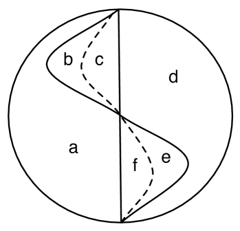
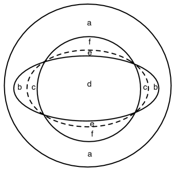
Figure 2. Schematic illustration of the interface perturbations and extensions for two different cases of the interface problem. The unperturbed interfaces $\Gamma$ are the vertical diameter (left) and the inner circle (right) respectively, while the perturbed interfaces $\Gamma_{\varepsilon}$ are the dashed lines for both cases. The unperturbed, $\varepsilon$-perturbed and $\varepsilon_{0}$-perturbed subdomains are respectively ${D}^{+}=a\cup b\cup c$, ${D}^{-}=d\cup e\cup f$; ${D}^{+}_{\varepsilon}=a\cup b\cup f$, ${D}^{-}_{\varepsilon}=d\cup c\cup e$; ${D}^{+}_{\varepsilon_{0}}=a\cup e\cup f$, ${D}^{-}_{\varepsilon_{0}}=d\cup b\cup c$. $u^{\pm}_{\varepsilon}$ are extended to the sufficiently large fixed domains ${D}^{+}\cup{D}^{+}_{\varepsilon_{0}}=a\cup b\cup c\cup e\cup f$ and ${D}^{-}\cup{D}^{-}_{\varepsilon_{0}}=d\cup b\cup c\cup e\cup f$ respectively. The Cauchy problems for $\tilde{u}_{\varepsilon}^{\pm}$ are imposed in the thin layers $\triangle_{\varepsilon}^{+}=c\cup e$ and $\triangle_{\varepsilon}^{-}=b\cup f$ respectively.

The first technical issue when applying the Taylor expansion is how to extend the solutions $u^{\pm}_{\varepsilon}$ of (5.4) from their own subdomains ${D}_{\varepsilon}^{\pm}$ onto the larger and fixed domains which both include the interface $\Gamma_{\varepsilon}$ for all $\varepsilon\in[0,\varepsilon_{0}]$. Such domains are chosen as ${D}^{\pm}\cup{D}_{\varepsilon_{0}}^{\pm}$. On these fixed domains ${D}^{\pm}\cup{D}_{\varepsilon_{0}}^{\pm}$, $u^{\pm}_{\varepsilon}$ are known on the parts $\overline{{D}_{\varepsilon}^{\pm}}$; we thus consider the differences $\triangle_{\varepsilon}^{\pm}$ which consist of the disjoint thin layers:

$$\triangle_{\varepsilon}^{\pm}:=({D}^{\pm}\cup{D}_{\varepsilon_{0}}^{\pm})\setminus\overline{{D}_{\varepsilon}^{\pm}}=({D}^{\pm}\setminus\overline{{D}_{\varepsilon}^{\pm}})\cup({D}_{\varepsilon_{0}}^{\pm}\setminus\overline{{D}_{\varepsilon}^{\pm}}).$$

Refer to Figure 2. Denote the solution extended on $\triangle_{\varepsilon}^{\pm}$ by $\tilde{u}_{\varepsilon}^{\pm}$, and assume that $\tilde{u}_{\varepsilon}^{\pm}$ and $u_{\varepsilon}^{\pm}$ have the same values and the same normal derivatives on the common boundary $\Gamma_{\varepsilon}$. Specifically, $\tilde{u}_{\varepsilon}^{\pm}$ are constructed as the unique solutions to the following Cauchy problems posed in the thin layers ${D}^{\pm}\setminus\overline{{D}_{\varepsilon}^{\pm}}$ and ${D}_{\varepsilon_{0}}^{\pm}\setminus\overline{{D}_{\varepsilon}^{\pm}}$ respectively:

$$\begin{cases}-\nabla\cdot\left(\sigma(\boldsymbol{x})\nabla\tilde{u}_{\varepsilon}^{\pm}(\boldsymbol{x})\right)=f(\boldsymbol{x})\qquad&\text{in }\triangle_{\varepsilon}^{\pm}=({D}^{\pm}\setminus\overline{{D}_{\varepsilon}^{\pm}})\cup({D}_{\varepsilon_{0}}^{\pm}\setminus\overline{{D}_{\varepsilon}^{\pm}}),\\ \tilde{u}_{\varepsilon}^{\pm}=u_{\varepsilon}^{\pm},\quad\partial_{\boldsymbol{n}}\tilde{u}_{\varepsilon}^{\pm}=\partial_{\boldsymbol{n}}u_{\varepsilon}^{\pm}\quad&\text{on }\Gamma_{\varepsilon},\end{cases}$$

where $u_{\varepsilon}^{\pm}$, the solution to equation (5.4), are presumably given. As in Section 2.1.1, the Cauchy-Kovalevskaya theorem [7] guarantees that such extensions can be realized analytically for sufficiently small $\varepsilon_{0}$ so that the Taylor expansion can be applied in a neighbourhood of $\Gamma$.

5.1.2. Asymptotic expansions on the fixed subdomains ${D}^{\pm}$

For ease of notation, we will still use $u^{\pm}_{\varepsilon}$ to denote their extensions defined above. Let us consider

$$u^{\pm}_{\varepsilon}=u_{0}^{\pm}+\varepsilon u_{1}^{\pm}+\varepsilon^{2}u_{2}^{\pm}+\ldots.$$ (5.6)

First, for the transmission condition $u_{\varepsilon}^{+}=u_{\varepsilon}^{-}$ on $\Gamma_{\varepsilon}$ in (5.3), by (5.2) we have

$$u^{+}_{\varepsilon}(\boldsymbol{x}+\varepsilon h(\boldsymbol{x})\boldsymbol{n}(\boldsymbol{x}))=u^{-}_{\varepsilon}(\boldsymbol{x}+\varepsilon h(\boldsymbol{x})\boldsymbol{n}(\boldsymbol{x})),\quad\boldsymbol{x}\in\Gamma,$$

and by (5.6), we have

$$\sum_{n=0}^{\infty}\varepsilon^{n}u^{+}_{n}(\boldsymbol{x}+\varepsilon h(\boldsymbol{x})\boldsymbol{n}(\boldsymbol{x}))=\sum_{n=0}^{\infty}\varepsilon^{n}u^{-}_{n}(\boldsymbol{x}+\varepsilon h(\boldsymbol{x})\boldsymbol{n}(\boldsymbol{x})),\quad\boldsymbol{x}\in\Gamma.$$

Then the Taylor expansions in $\varepsilon$ on both sides as before can yield

$$\sum_{k=0}^{n}\frac{(h(\boldsymbol{x}))^{k}}{k!}{\partial_{\boldsymbol{n}}^{k}}u^{+}_{n-k}(\boldsymbol{x})=\sum_{k=0}^{n}\frac{(h(\boldsymbol{x}))^{k}}{k!}{\partial_{\boldsymbol{n}}^{k}}u^{-}_{n-k}(\boldsymbol{x}),\quad\boldsymbol{x}\in\Gamma,$$

thus

$$\left[u_{n}(\boldsymbol{x})\right]=-\sum_{k=1}^{n}\frac{(h(\boldsymbol{x}))^{k}}{k!}\left[{\partial_{\boldsymbol{n}}^{k}}u_{n-k}(\boldsymbol{x})\right]\quad\text{on }{\Gamma},$$ (5.7)

where $\left[v\right]:=v^{+}-v^{-}$ deontes the jump across the subdomains from ${D}^{-}$ to ${D}^{+}$.

On the other hand, from the variational form (5.4), we obtain

$$\begin{split}&\int_{{D}^{+}}\sigma^{+}\nabla u^{+}_{\varepsilon}\cdot\nabla v\,\mathrm{d}\boldsymbol{x}+\int_{{D}^{-}}\sigma^{-}\nabla u^{-}_{\varepsilon}\cdot\nabla v\,\mathrm{d}\boldsymbol{x}\\ &-\int_{\delta{D}_{\varepsilon}}\sigma^{+}\nabla u^{+}_{\varepsilon}\cdot\nabla v\,\mathrm{d}\boldsymbol{x}+\int_{\delta{D}_{\varepsilon}}\sigma^{-}\nabla u^{-}_{\varepsilon}\cdot\nabla v\,\mathrm{d}\boldsymbol{x}=\int_{{D}}fv\,\mathrm{d}\boldsymbol{x},\end{split}$$ (5.8)

where $\delta{D}_{\varepsilon}=({D}_{\varepsilon}^{+}\setminus{D}^{+})\cup({D}^{+}\setminus{D}_{\varepsilon}^{+})=({D}^{-}\setminus{D}_{\varepsilon}^{-})\cup({D}^{-}_{\varepsilon}\setminus{D}^{-})$, and the integrand on $\delta{D}_{\varepsilon}$ is taken with a minus sign over ${D}_{\varepsilon}^{+}\setminus{D}^{+}={D}^{-}\setminus{D}_{\varepsilon}^{-}$ and a plus sign over ${D}^{+}\setminus{D}_{\varepsilon}^{+}={D}^{-}_{\varepsilon}\setminus{D}^{-}$. Note that

$${D}^{+}\setminus{D}_{\varepsilon}^{+}={D}^{-}_{\varepsilon}\setminus{D}^{-}=\left\{\boldsymbol{x}+t\boldsymbol{n}(\boldsymbol{x}):\boldsymbol{x}\in\Gamma,~{}h(\boldsymbol{x})>0,~{}0\leqslant t<\varepsilon h(\boldsymbol{x})\right\},$$

$${D}_{\varepsilon}^{+}\setminus{D}^{+}={D}^{-}\setminus{D}_{\varepsilon}^{-}=\left\{\boldsymbol{x}+t\boldsymbol{n}(\boldsymbol{x}):\boldsymbol{x}\in\Gamma,~{}h(\boldsymbol{x})<0,~{}\varepsilon h(\boldsymbol{x})<t\leqslant 0\right\}.$$

To handle the integration $\int_{\delta{D}_{\varepsilon}}$ in (5.8), we introduce the curvilinear coordinates $(\boldsymbol{\xi},t)$ in a sufficiently small tubular neighborhood of $\Gamma$, which are defined by

$$\boldsymbol{x}=\boldsymbol{\theta}(\boldsymbol{\xi})+t\boldsymbol{n}(\boldsymbol{\xi}),$$

where $\boldsymbol{\xi}=(\xi_{1},\cdots,\xi_{d-1})\in\Omega\longmapsto\boldsymbol{\theta}(\boldsymbol{\xi})\in\Gamma$ is a parametrization of the interface $\Gamma$ and $\boldsymbol{n}(\boldsymbol{\xi}):=\boldsymbol{n}(\boldsymbol{\theta}(\boldsymbol{\xi}))$. Then for any smooth function $g$, by making use of a change of variables, we have

$$\begin{split}\int_{\delta{D}_{\varepsilon}}g(\boldsymbol{x})\,\mathrm{d}\boldsymbol{x}=&\int_{\Omega}\biggl{(}\int_{0}^{\varepsilon h(\boldsymbol{\theta}(\boldsymbol{\xi}))}g(\boldsymbol{\theta}(\boldsymbol{\xi})+t\boldsymbol{n}(\boldsymbol{\xi}))\lvert J(\boldsymbol{\xi},t)\rvert\,\mathrm{d}t\biggr{)}\mathrm{d}{\boldsymbol{\xi}},\end{split}$$ (5.9)

where $J(\boldsymbol{\xi},t)$ is the Jacobian determinant of the mapping $(\boldsymbol{\xi},t)\longmapsto\boldsymbol{x}$. By Appendix B.3, (5.9) is equivalent to

$$\int_{\delta{D}_{\varepsilon}}g(\boldsymbol{x})\,\mathrm{d}\boldsymbol{x}=\int_{\Gamma}\biggl{(}\int_{0}^{\varepsilon h(\boldsymbol{\theta})}\tilde{g}(\boldsymbol{\theta},t)\det(I+tW)\,\mathrm{d}t\biggr{)}\mathrm{d}S_{\Gamma}({\boldsymbol{\theta}}),$$ (5.10)

where $\tilde{g}(\boldsymbol{\theta},t):=g(\boldsymbol{\theta}+t\boldsymbol{n}(\boldsymbol{\theta}))$, $\boldsymbol{\theta}\in\Gamma$, $I$ denotes the identity matrix, $W=(W_{i}^{~{}j})$ is the matrix representation of the Weingarten map, and $\mathrm{d}S_{\Gamma}(\boldsymbol{\theta})$ denotes the surface area element on the hypersurface $\Gamma$.

The equality (5.10) is the major foundation to apply the asymptotic expansion. We show how to proceed this task by considering the first two orders $u^{\pm}_{0}$ and $u^{\pm}_{1}$. Since

$$\tilde{g}(\boldsymbol{\theta},t)\det(I+tW)=\tilde{g}(\boldsymbol{\theta},0)+\mathcal{O}(t)=g(\boldsymbol{\theta})+\mathcal{O}(t),$$ (5.11)

then

$$\begin{split}\int_{\delta{D}_{\varepsilon}}g(\boldsymbol{x})\,\mathrm{d}\boldsymbol{x}=&~{}\varepsilon\int_{\Gamma}h(\boldsymbol{\theta})g(\boldsymbol{\theta})\,\mathrm{d}S_{\Gamma}({\boldsymbol{\theta}})+\mathcal{O}(\varepsilon^{2}).\end{split}$$ (5.12)

Note that on $\Gamma$, we have the following orthogonal decomposition of the gradient operator:

$$\nabla=\nabla_{\Gamma}+\boldsymbol{n}\partial_{\boldsymbol{n}},$$

where $\nabla_{\Gamma}$ denotes the surface gradient operator. Then

$$\left[\sigma\nabla u_{k}\right]\cdot\nabla v=\left[\sigma\nabla_{\Gamma}u_{k}\right]\cdot\nabla_{\Gamma}v+\left[\sigma\partial_{\boldsymbol{n}}u_{k}\right]\partial_{\boldsymbol{n}}v\quad\text{on }\Gamma.$$ (5.13)

Substituting (5.6) into (5.8), and applying (5.12) and (5.13), we are led to

$$\begin{split}&\sum_{n=0}^{1}\varepsilon^{n}\int_{{D}^{+}}\sigma^{+}\nabla u^{+}_{n}\cdot\nabla v\,\mathrm{d}\boldsymbol{x}+\sum_{n=0}^{1}\varepsilon^{n}\int_{{D}^{-}}\sigma^{-}\nabla u^{-}_{n}\cdot\nabla v\,\mathrm{d}\boldsymbol{x}\\ &-\varepsilon\int_{\Gamma}h\bigl{(}\left[\sigma\nabla_{\Gamma}u_{0}\right]\cdot\nabla_{\Gamma}v+\left[\sigma\partial_{\boldsymbol{n}}u_{0}\right]\partial_{\boldsymbol{n}}v\bigr{)}\,\mathrm{d}S_{\Gamma}+\mathcal{O}(\varepsilon^{2})=\int_{{D}}fv\,\mathrm{d}\boldsymbol{x}.\end{split}$$

Now we collect terms with equal powers of $\varepsilon$ and obtain:

$$\int_{{D}^{+}}\sigma^{+}\nabla u^{+}_{0}\cdot\nabla v\,\mathrm{d}\boldsymbol{x}+\int_{{D}^{-}}\sigma^{-}\nabla u^{-}_{0}\cdot\nabla v\,\mathrm{d}\boldsymbol{x}=\int_{{D}}fv\,\mathrm{d}\boldsymbol{x};$$ (5.14)

$$\begin{split}&\int_{{D}^{+}}\sigma^{+}\nabla u^{+}_{1}\cdot\nabla v\,\mathrm{d}\boldsymbol{x}+\int_{{D}^{-}}\sigma^{-}\nabla u^{-}_{1}\cdot\nabla v\,\mathrm{d}\boldsymbol{x}\\ &-\int_{\Gamma}h\bigl{(}\left[\sigma\nabla_{\Gamma}u_{0}\right]\cdot\nabla_{\Gamma}v+\left[\sigma\partial_{\boldsymbol{n}}u_{0}\right]\partial_{\boldsymbol{n}}v\bigr{)}\,\mathrm{d}S_{\Gamma}=0\quad\forall v\in H_{0}^{1}({D}).\end{split}$$ (5.15)

These weak formulations together with (5.7) with $n=0,1$, lead to the following two PDEs for $u_{0}$ and $u_{1}$, respectively:

$$\begin{cases}&-\nabla\cdot\left(\sigma(\boldsymbol{x})\nabla u_{0}(\boldsymbol{x})\right)=f(\boldsymbol{x})\quad\text{in }{{D}^{+}}\cup{D}^{-},\\ &\left[u_{0}(\boldsymbol{x})\right]=\displaystyle\left[\sigma(\boldsymbol{x})\partial_{\boldsymbol{n}}u_{0}(\boldsymbol{x})\right]=0\quad\text{on }{\Gamma},\\ &u=g\quad\text{on }\partial{D}.\end{cases}$$ (5.16)

and

$$\begin{cases}&-\nabla\cdot\left(\sigma(\boldsymbol{x})\nabla u_{1}(\boldsymbol{x})\right)=0\quad\text{in }{{D}^{+}}\cup{D}^{-},\\ &\left[u_{1}\right]=-h\left[\partial_{\boldsymbol{n}}u_{0}\right],\quad\displaystyle\left[\sigma\partial_{\boldsymbol{n}}u_{1}\right]=\nabla_{\Gamma}\cdot(h\left[\sigma\right]\nabla_{\Gamma}u_{0})\quad\text{on }{\Gamma},\\ &u_{1}=0\quad\text{on }\partial{D}.\end{cases}$$ (5.17)

The equations for higher order terms, $u_{n},n\geqslant 2$, can be derived in the same way by considering the higher order Taylor approximations for (5.11).

5.2. Two-parameter expansions

The expansion of high-contrast ratio without interface perturbation is derived in [1]. In the sequel, we show the two-parameter expansion results by combining our $\varepsilon$ expansion and the $\sigma$-expansion in [1]. We need to consider the following two different cases:

• $\varepsilon\rightarrow 0,\sigma\rightarrow\infty$,

• $\varepsilon\rightarrow 0,\sigma\rightarrow 0$.

Note that $\sigma$ is defined on the subdomain ${D}_{\varepsilon}^{-}$ by (5.5). For Case (i), the solution is still bounded; for Case (ii), the solution on ${D}^{-}_{\varepsilon}$ behaves at the order $\mathcal{O}(1/\sigma)$. The difference between these two cases is mainly a scaling factor $1/\sigma$. We focus on Case (i) here. The derivation for Case (ii) can be found in Appendix C.

In Case (i), we have $\varepsilon\to 0$ and $\sigma\to+\infty$. We introduce $\mu=1/\sigma$ and treat $\varepsilon$ and $\mu$ as independent small parameters. Assume $u^{+}_{\varepsilon}$ and $u^{-}_{\varepsilon}$ have double asymptotic expansions

$$u^{\pm}_{\varepsilon}(\boldsymbol{x})=\sum_{m,n=0}^{\infty}u^{\pm}_{m,n}(\boldsymbol{x})\varepsilon^{m}\mu^{n},\quad\boldsymbol{x}\in{D}^{\pm},$$

and introduce the notation

$$u^{\pm}_{m,\cdot}(\boldsymbol{x})=\sum_{n=0}^{\infty}u^{\pm}_{m,n}(\boldsymbol{x})\mu^{n},\quad\boldsymbol{x}\in{D}^{\pm},$$ (5.18)

From the condition (5.7) we obtain

$$\left[u_{0,\cdot}\right]=0,\quad\left[u_{1,\cdot}\right]=-h\left[{\partial_{\boldsymbol{n}}}u_{0,\cdot}\right]\quad\text{on }{\Gamma},$$ (5.19)

Substituting (5.18) into (5.19) and matching the terms with the same order of $\mu$ yield that

$$u^{-}_{0,n}=u^{+}_{0,n},\quad n\geqslant 0,$$ (5.20)

$$u^{-}_{1,n}=u^{+}_{1,n}+h\left[{\partial_{\boldsymbol{n}}}u_{0,n}\right]\quad n\geqslant 0.$$ (5.21)

For the piecewisely homogeneous case of $\sigma$ considered here, (5.14) and (5.15) become that for all $v\in H_{0}^{1}({D})$,

$$\int_{{D}^{+}}\nabla u^{+}_{0,\cdot}\cdot\nabla v\,\mathrm{d}\boldsymbol{x}+\int_{{D}^{-}}\sigma\nabla u^{-}_{0,\cdot}\cdot\nabla v\,\mathrm{d}\boldsymbol{x}=\int_{{D}}fv\,\mathrm{d}\boldsymbol{x};$$ (5.22)

$$\int_{{D}^{+}}\nabla u^{+}_{1,\cdot}\cdot\nabla v\,\mathrm{d}\boldsymbol{x}+\int_{{D}^{-}}\sigma\nabla u^{-}_{1,\cdot}\cdot\nabla v\,\mathrm{d}\boldsymbol{x}$$

$$-\int_{\Gamma}h\bigl{[}(\nabla_{\Gamma}u^{+}_{0,\cdot}-\sigma\nabla_{\Gamma}u^{-}_{0,\cdot})\cdot\nabla_{\Gamma}v+(\partial_{\boldsymbol{n}}u^{+}_{0,\cdot}-\sigma\partial_{\boldsymbol{n}}u^{-}_{0,\cdot})\partial_{\boldsymbol{n}}v\bigr{]}\,\mathrm{d}S_{\Gamma}=0.$$ (5.23)

Substituting (5.18) into (5.22) and (5.23), we have that for all $v\in H_{0}^{1}({D})$,

$$\int_{{D}^{-}}\nabla u^{-}_{0,0}\cdot\nabla v\,\mathrm{d}\boldsymbol{x}=0,$$ (5.24)

$$\int_{{D}^{-}}\nabla u^{-}_{1,0}\cdot\nabla v\,\mathrm{d}\boldsymbol{x}=\int_{\Gamma}h\bigl{[}\nabla_{\Gamma}u^{-}_{0,0}\cdot\nabla_{\Gamma}v+\partial_{\boldsymbol{n}}u^{-}_{0,0}\partial_{\boldsymbol{n}}v\bigr{]}\,\mathrm{d}S_{\Gamma},$$ (5.25)

and for $n\geqslant 0$,

$$\int_{{D}^{+}}\nabla u^{+}_{0,n}\cdot\nabla v\,\mathrm{d}\boldsymbol{x}+\int_{{D}^{-}}\nabla u^{-}_{0,n+1}\cdot\nabla v\,\mathrm{d}\boldsymbol{x}=\delta_{0,n}\int_{{D}}fv\,\mathrm{d}\boldsymbol{x};$$ (5.26)

$$\int_{{D}^{+}}\nabla u^{+}_{1,n}\cdot\nabla v\,\mathrm{d}\boldsymbol{x}+\int_{{D}^{-}}\nabla u^{-}_{1,n+1}\cdot\nabla v\,\mathrm{d}\boldsymbol{x}$$

$$-\int_{\Gamma}h\bigl{[}(\nabla_{\Gamma}u^{+}_{0,n}-\nabla_{\Gamma}u^{-}_{0,n+1})\cdot\nabla_{\Gamma}v+(\partial_{\boldsymbol{n}}u^{+}_{0,n}-\partial_{\boldsymbol{n}}u^{-}_{0,n+1})\partial_{\boldsymbol{n}}v\bigr{]}\,\mathrm{d}S_{\Gamma}=0.$$ (5.27)

From (5.20) and the weak formulation (5.24) (5.26), we have the following PDEs for each term:

$$\begin{cases}&-\Delta u^{-}_{0,0}=0\quad\text{in }{D}^{-},\\ &\partial_{\boldsymbol{n}}u^{-}_{0,0}=0\quad\text{on }\Gamma,\\ &u^{-}_{0,0}=g\quad\text{on }\partial{D}^{-}\cap\partial{D};\end{cases}$$ (5.28)

and for $n\geqslant 0$,

$$\begin{cases}&-\Delta u^{+}_{0,n}=\delta_{0,n}f\quad\text{in }{D}^{+},\\ &u^{+}_{0,n}=u^{-}_{0,n}\quad\text{on }\Gamma,\\ &u^{+}_{0,n}=\delta_{0,n}g\quad\text{on }\partial{D}^{+}\cap\partial{D};\end{cases}$$ (5.29)

and for $n\geqslant 1$,

$$\begin{cases}&-\Delta u^{-}_{0,n}=\delta_{1,n}f\quad\text{in }{D}^{-},\\ &\partial_{\boldsymbol{n}}u^{-}_{0,n}=\partial_{\boldsymbol{n}}u^{+}_{0,n-1}\quad\text{on }\Gamma,\\ &u^{-}_{0,n}=0\quad\text{on }\partial{D}^{-}\cap\partial{D}.\end{cases}$$ (5.30)

We also list the PDEs for the terms with $m=1$:

$$\begin{cases}&-\Delta u^{-}_{1,0}=0\quad\text{in }{D}^{-},\\ &\partial_{\boldsymbol{n}}u^{-}_{1,0}=-\nabla_{\Gamma}\cdot(h\nabla_{\Gamma}u^{-}_{0,0})\quad\text{on }\Gamma,\\ &u^{-}_{1,0}=0\quad\text{on }\partial{D}^{-}\cap\partial{D};\end{cases}$$

and for $n\geqslant 0$,

$$\begin{cases}&-\Delta u^{+}_{1,n}=0\quad\text{in }{D}^{+},\\ &u^{+}_{1,n}=u^{-}_{1,n}-h(\partial_{\boldsymbol{n}}u^{+}_{0,n}-\partial_{\boldsymbol{n}}u^{-}_{0,n})\quad\text{on }\Gamma,\\ &u^{+}_{1,n}=0\quad\text{on }\partial{D}^{+}\cap\partial{D};\end{cases}$$

and

$$\begin{cases}&-\Delta u^{-}_{1,n}=0\quad\text{in }{D}^{-},\\ &\partial_{\boldsymbol{n}}u^{-}_{1,n}=\partial_{\boldsymbol{n}}u^{+}_{1,n-1}+\nabla_{\Gamma}\cdot\bigl{[}h(\nabla_{\Gamma}u^{+}_{0,n-1}-\nabla_{\Gamma}u^{-}_{0,n})\bigr{]}\quad\text{on }\Gamma,\\ &u^{-}_{1,n}=0\quad\text{on }\partial{D}^{-}\cap\partial{D}.\end{cases}$$

Here we need to pay attention to a special situation that $\partial{D}^{-}=\Gamma$, or equivalently, $\partial{D}^{-}\cap\partial{D}=\emptyset$. Refer to the right panel in Figure 2. The boundary value problems above then may become Neumann problems, which are uniquely solvable only up to an arbitrary constant. To determine those constants, as we have done in Section 4.2.2, we need the solvability condition from the next order. For $m=0$, and $n\geqslant 1$, the solvability condition for (5.30) reads

$$\int_{\Gamma}\partial_{\boldsymbol{n}}u^{+}_{0,n-1}\,\mathrm{d}S_{\Gamma}=-\delta_{1,n}\int_{{D}^{-}}f\,\mathrm{d}\boldsymbol{x}.$$ (5.31)

(5.28) shows that $u^{-}_{0,0}\equiv C_{0}$. To determine $C_{0}$, we need to look at $u^{+}_{0,0}$, which satisfies

$$\begin{cases}&-\Delta u^{+}_{0,0}=f\quad\text{in }{D}^{+},\\ &u^{+}_{0,0}=C_{0}\quad\text{on }\Gamma,\\ &u^{+}_{0,0}=g\quad\text{on }\partial{D},\\ \end{cases}$$ (5.32)

by (5.29). By the solvability condition (5.31), we have $\int_{\Gamma}\partial_{\boldsymbol{n}}u^{+}_{0,0}\,\mathrm{d}S_{\Gamma}=-\int_{{D}^{-}}f\,\mathrm{d}\boldsymbol{x}$, which uniquely determines the constant

$$C_{0}=-\frac{\int_{{D}^{-}}f+\int_{\Gamma}(\partial_{\boldsymbol{n}}\phi_{2}+\partial_{\boldsymbol{n}}\phi_{3})}{\int_{\Gamma}\partial_{\boldsymbol{n}}\phi_{1}},$$

where $\phi_{i}$ solve the following equations, respectively,

$$\begin{cases}&-\Delta\phi_{1}=0\quad\text{in }{D}^{+},\\ &\phi_{1}=1\quad\text{on }\Gamma,\\ &\phi_{1}=0\quad\text{on }\partial{D},\\ \end{cases}~{}~{}\begin{cases}&-\Delta\phi_{2}=f\quad\text{in }{D}^{+},\\ &\phi_{2}=0\quad\text{on }\Gamma,\\ &\phi_{2}=0\quad\text{on }\partial{D},\\ \end{cases}~{}~{}\begin{cases}&-\Delta\phi_{3}=0\quad\text{in }{D}^{+},\\ &\phi_{3}=0\quad\text{on }\Gamma,\\ &\phi_{3}=g\quad\text{on }\partial{D}.\\ \end{cases}$$ (5.33)

Acknowledgment. J. Chen acknowledges support from National Natural Science Foundation of China grant 21602149. L. Lin and X. Zhou acknowledge the financial support of Hong Kong GRF (109113, 11304314, 11304715). Z. Zhang acknowledges the financial support of Hong Kong RGC grants (27300616, 17300817) and National Natural Science Foundation of China via grant 11601457. J. Chen would like to thank the hospitality of Department of Mathematics, City University of Hong Kong where part of the work was done.

Appendix A Examples and generalizations for Section 2

A.1. Two examples

The following two 2D examples demonstrate how the explicit form of the operator $F_{k,\Gamma,\mathcal{L},f}$ can be obtained in Lemma 2.3.

Example A.1.

Consider

$$\mathcal{L}u=-\sigma\partial_{x}^{2}u-\sigma\partial_{y}^{2}u+cu$$

over ${D}=(0,~{}L_{1})\times(0,~{}L_{2})$ with constants $\sigma>0$, $c\geqslant 0$ and the homogeneous Dirichlet boundary condition $g=0$. Suppose the domain perturbation is only applied to the right boundary $\Gamma=\left\{(L_{1},y):0\leqslant y\leqslant L_{2}\right\}$ in the following form

$$\Gamma_{\varepsilon}=\left\{(L_{1}+\varepsilon h(y),y):0\leqslant y\leqslant L_{2}\right\}.$$ (A.1)

Then, $\partial_{\boldsymbol{n}}^{k}=\partial_{x}^{k}$, $\forall k\geqslant 0$. The conversion of all partial derivatives of a function $w(x,y)$ with respect to $x$ with $k\geqslant 2$ to the partial derivatives with respect to $y$ relies on the repeated use of the partial differential equation

$$\mathcal{L}w=-\sigma\partial_{x}^{2}w-\sigma\partial_{y}^{2}w+cw=\phi.$$ (A.2)

Explicit forms when $k=2$ and $k=3$ are as follows.

1. From (A.2), we have

   $$\partial_{x}^{2}w=-\frac{\phi}{\sigma}+\frac{cw}{\sigma}-\partial_{y}^{2}w,$$ (A.3)

   which implies

   $$F_{2,\phi}[g_{0},g_{1}]=-\frac{\phi}{\sigma}+\frac{cg_{0}}{\sigma}-\partial_{y}^{2}g_{0}.$$

2. Differentiating (A.2) with respect to $x$ yields

   $$-\sigma\partial_{x}^{3}w-\sigma\partial_{y}^{2}\partial_{x}w+c\partial_{x}w=\partial_{x}\phi,$$

   and thus

   $$\partial_{x}^{3}w=\frac{1}{\sigma}\left(-\sigma\partial_{y}^{2}\partial_{x}w+c\partial_{x}w-\partial_{x}\phi\right),$$ (A.4)

   which implies

   $$F_{3,\phi}[g_{0},g_{1}]=\frac{1}{\sigma}\left(-\sigma\partial_{y}^{2}g_{1}+cg_{1}-\partial_{x}\phi\right).$$

Using the above formulas, we can convert all partial derivatives of $u_{0}$ and $u_{1}$ with $k=2$ and $k=3$ in (2.14) and (2.15) to the partial derivatives with respect to $y$ with the following explicit forms.

1. Using $u_{0}(L_{1},y)=0,\;0\leqslant y\leqslant L_{2}$ for $u_{0}$ in (A.3), we have

   $$\partial_{x}^{2}u_{0}(L_{1},y)=-\frac{1}{\sigma}f(L_{1},y).$$

   Solving $\mathcal{L}u_{1}=0$ produces

   $$\partial_{x}^{2}u_{1}(L_{1},y)=\frac{cu_{1}(L_{1},y)}{\sigma}-\partial^{2}_{y}u_{1}(L_{1},y).$$

2. Substituting $u_{0}(x,y)$ into (A.4) and evaluating at $x=L_{1}$ yield

   $$\partial_{x}^{3}u_{0}(L_{1},y)=\frac{1}{\sigma}\left(-\sigma\partial_{y}^{2}\partial_{x}u_{0}(L_{1},y)+c\partial_{x}u_{0}(L_{1},y)-\partial_{x}f(L_{1},y)\right).$$

Example A.2.

Consider

$$\mathcal{L}=-\nabla\cdot\bigl{(}\sigma(\boldsymbol{x})\nabla)\bigr{)}=-\sigma\Delta-\nabla\sigma\cdot\nabla$$

in 2D with the scalar-valued smooth function $\sigma>0$ and set $g=0$. Assume the 1D boundary $\partial{D}$ has a parametrization by the arc length $s\mapsto\boldsymbol{\theta}(s)$. Then at each point $\boldsymbol{\theta}(s)$, the unit tangent vector $\boldsymbol{\tau}(s)$ is $\boldsymbol{\theta}^{\prime}(s)$ and the curvature $\kappa(s)$ is defined as

$$\boldsymbol{\tau}^{\prime}(s)=-\kappa(s)\boldsymbol{n}(s),~{}\text{ equivalently, }~{}\kappa(s)=\boldsymbol{\tau}(s)\cdot\boldsymbol{n}^{\prime}(s).$$

In a sufficiently small tubular neighborhood of $\partial{D}$, the curvilinear coordinates $(s,t)$ are uniquely defined by $\boldsymbol{x}=\boldsymbol{\theta}(s)+t\boldsymbol{n}(s)$. The gradient and the Laplace operators in curvilinear coordinates are

$$\nabla=\boldsymbol{\tau}(s)\frac{1}{1+t\kappa(s)}\partial_{s}+\boldsymbol{n}(s)\partial_{t},$$

and

$$\Delta=\frac{1}{1+t\kappa(s)}\partial_{s}\left(\frac{1}{1+t\kappa(s)}\partial_{s}\right)+\frac{\kappa(s)}{1+t\kappa(s)}\partial_{t}+\partial_{t}^{2},$$

respectively.

Then the operator $\mathcal{L}$ has the new form in terms of $(s,t)$,

$$\begin{split}\mathcal{L}u=&-\frac{\sigma}{1+t\kappa(s)}\partial_{s}\left(\frac{1}{1+t\kappa(s)}\partial_{s}u\right)-\frac{\sigma\kappa(s)}{1+t\kappa(s)}\partial_{t}u\\ &-\sigma\partial_{t}^{2}u-\frac{\partial_{t}\sigma\partial_{s}u}{1+t\kappa(s)}-\partial_{\boldsymbol{n}}\sigma\partial_{t}u.\end{split}$$ (A.5)

Note that $\partial_{\boldsymbol{n}}^{k}=\partial_{t}^{k}$, $\forall k\geqslant 0$.

Explicit forms for $F_{2,\phi}[\cdot,\cdot]$ and $F_{3,\phi}[\cdot,\cdot]$ are as follows.

1. Consider the equation $\mathcal{L}w=\phi$ on $\partial{D}$ (i.e., $t=0$ )

   $$-\sigma(\partial^{2}_{s}w+\kappa\partial_{\boldsymbol{n}}w+\partial_{\boldsymbol{n}}^{2}w)-\partial_{s}\sigma\partial_{s}w-\partial_{\boldsymbol{n}}\sigma\partial_{\boldsymbol{n}}w=\phi,$$

   which implies

   $$\partial_{\boldsymbol{n}}^{2}w=-\frac{\phi}{\sigma}-\frac{\partial_{s}\sigma}{\sigma}\partial_{s}w-\frac{\partial_{\boldsymbol{n}}\sigma}{\sigma}\partial_{\boldsymbol{n}}w-\partial^{2}_{s}w-\kappa\partial_{\boldsymbol{n}}w.$$ (A.6)

   Thus

   $$F_{2,\phi}[g_{0},g_{1}]=-\frac{\phi}{\sigma}-\frac{\partial_{s}\sigma}{\sigma}\partial_{s}g_{0}-\frac{\partial_{\boldsymbol{n}}\sigma}{\sigma}g_{1}-\partial^{2}_{s}g_{0}-\kappa g_{1}.$$

2. For simplicity we assume constant coefficient $\sigma$ in the following calculation. Differentiating the equation $\mathcal{L}w=\phi$ with respect to $t$ at $t=0$ yields

   $$\begin{split}&\sigma(\kappa^{\prime}\partial_{s}+2\kappa\partial_{s}^{2}-\partial_{s}^{2}\partial_{t}+\kappa^{2}\partial_{t}-\kappa\partial_{t}^{2}-\partial_{t}^{3})w=\partial_{t}\phi.\end{split}$$

   Thus,

   $$\begin{split}\partial_{\boldsymbol{n}}^{3}w=&(\kappa^{\prime}\partial_{s}+2\kappa\partial_{s}^{2}-\partial_{s}^{2}\partial_{\boldsymbol{n}}+\kappa^{2}\partial_{\boldsymbol{n}}-\kappa\partial_{\boldsymbol{n}}^{2})w-\frac{\partial_{\boldsymbol{n}}\phi}{\sigma}\\ =&(\kappa^{\prime}\partial_{s}+3\kappa\partial_{s}^{2}-\partial_{s}^{2}\partial_{\boldsymbol{n}}+2\kappa^{2}\partial_{\boldsymbol{n}})w-\frac{\partial_{\boldsymbol{n}}\phi}{\sigma}+\frac{\kappa\phi}{\sigma}.\end{split}$$ (A.7)

   In the last equality, we use (A.6) for $\partial_{\boldsymbol{n}}^{2}w$. Therefore

   $$F_{3,\phi}[g_{0},g_{1}]=(\kappa^{\prime}\partial_{s}+3\kappa\partial_{s}^{2})g_{0}+(2\kappa^{2}-\partial_{s}^{2})g_{1}+\frac{\kappa-\partial_{\boldsymbol{n}}}{\sigma}\phi.$$

Using the above formulas, we can convert all partial derivatives of $u_{0}$ and $u_{1}$ with $k=2$ and $k=3$ in (2.14) and (2.15) to the partial derivatives with respect to $y$ with the following explicit forms

1. On $\partial{D}$, from (A.6), we have

   $$\partial_{\boldsymbol{n}}^{2}u_{0}=-\frac{f}{\sigma}-\frac{\partial_{\boldsymbol{n}}\sigma}{\sigma}\partial_{\boldsymbol{n}}u_{0}-\kappa\partial_{\boldsymbol{n}}u_{0}.$$

   Thus the boundary condition (2.14) for $u_{2}$ on $\partial{D}$ is reduced to

   $$u_{2}=-h\partial_{\boldsymbol{n}}u_{1}+\frac{h^{2}}{2}\Bigl{(}\frac{\partial_{\boldsymbol{n}}\sigma}{\sigma}+\kappa\Bigr{)}\partial_{\boldsymbol{n}}u_{0}+\dfrac{h^{2}f}{2\sigma}.$$ (A.8)

   Similarly, for $n\geqslant 1$, we have on $\partial{D}$

   $$\partial_{\boldsymbol{n}}^{2}u_{n}=-\kappa\partial_{\boldsymbol{n}}u_{n}-\frac{\partial_{\boldsymbol{n}}\sigma}{\sigma}\partial_{\boldsymbol{n}}u_{n}-\frac{\partial_{s}\sigma}{\sigma}\partial_{s}u_{n}-\partial^{2}_{s}u_{n}.$$

2. From (A.7), we have on $\partial{D}$

   $$\begin{split}\partial_{\boldsymbol{n}}^{3}u_{n}=&F_{3,\delta_{0,n}f}[u_{n},\partial_{\boldsymbol{n}}{u_{n}}]\\ =&\delta_{0,n}\frac{\kappa-\partial_{\boldsymbol{n}}}{\sigma}f+(1-\delta_{0,n})\Bigl{(}\kappa^{\prime}\partial_{s}+3\kappa\partial_{s}^{2}\Bigr{)}u_{n}+\Bigl{(}2\kappa^{2}-\partial_{s}^{2}\Bigr{)}\partial_{\boldsymbol{n}}u_{n}.\end{split}$$

A.2. Neumann boundary conditions

If the Neumann boundary condition $\partial_{\boldsymbol{n}}u_{\varepsilon}=g$ rather than the Dirichlet boundary condition is prescribed on the boundary $\partial{D}_{\varepsilon}$ for the equation (1.2), the above method in $\S$2.1.2 still works straightforwardly. $w_{\varepsilon}=g$ in (2.4) becomes $\partial_{\boldsymbol{n}}w_{\varepsilon}=g$ on $\partial{D}_{\varepsilon}$ now. So (2.7) becomes

$$\sum_{n=0}^{\infty}\varepsilon^{n}\partial_{\boldsymbol{n}}w_{n}\bigl{(}\boldsymbol{x}+\varepsilon h(\boldsymbol{x})\boldsymbol{n}(x)\bigr{)}=g\bigl{(}\boldsymbol{x}+\varepsilon h(\boldsymbol{x})\boldsymbol{n}(x)\bigr{)}\quad\text{for }\boldsymbol{x}\in\partial{D}.$$

The Taylor expansions (2.8) and (2.9) are still applicable along the normal direction $\boldsymbol{n}$ and the new conditions corresponding to (2.10) can be obtained by following the previous procedure there.

For ease of exposition, let us just show the specific forms for Example A.1 when the homogeneous Neumann boundary condition is imposed on $\Gamma_{\varepsilon}$ defined in (A.1). The unit normal vector $\boldsymbol{n}(x,y)$ on $\Gamma_{\varepsilon}$ parallels to $(1,-\varepsilon h^{\prime}(y))$, thus $\sum_{n=0}^{\infty}\varepsilon^{n}\partial_{\boldsymbol{n}}w_{n}(x,y)=0$ on $\Gamma_{\varepsilon}$ is written as

$$\sum_{n=0}^{\infty}\varepsilon^{n}\Bigl{(}\partial_{x}w_{n}\bigl{(}L_{1}+\varepsilon h(y),y\bigr{)}-\varepsilon h^{\prime}(y)\partial_{y}w_{n}\bigl{(}L_{1}+\varepsilon h(y),y\bigr{)}\Bigr{)}=0.$$

Then the Taylor expansion gives arise to

$$\begin{split}&\sum_{m=0}^{\infty}\varepsilon^{m}\sum_{k=0}^{m}\frac{\bigl{(}h(y)\bigr{)}^{k}}{k!}\partial_{x}^{k+1}w_{m-k}(L_{1},y)=\\ &~{}\qquad\sum_{m=1}^{\infty}\varepsilon^{m}\sum_{k=0}^{m-1}\frac{\bigl{(}h(y)\bigr{)}^{k}}{k!}h^{\prime}(y)\partial_{x}^{k}\partial_{y}w_{m-1-k}(L_{1},y).\end{split}$$

Then after matching each order $\varepsilon^{m}$, we have that

$$\partial_{x}w_{0}(L_{1},y)=0,$$ (A.9)

and for $m\geqslant 1$,

$$\sum_{k=0}^{m}\frac{\bigl{(}h(y)\bigr{)}^{k}}{k!}\partial_{x}^{k+1}w_{m-k}(L_{1},y)=\sum_{k=0}^{m-1}\frac{\bigl{(}h(y)\bigr{)}^{k}}{k!}h^{\prime}(y)\partial_{x}^{k}\partial_{y}w_{m-1-k}(L_{1},y).$$

In particular, the boundary conditions for $m=1,2$ are

$$\partial_{x}w_{1}+h(y)\partial_{x}^{2}w_{0}-h^{\prime}(y)\partial_{y}w_{0}=0,$$

$$\partial_{x}w_{2}+h(y)\partial_{x}^{2}w_{1}+\frac{1}{2}\bigl{(}h(y)\bigr{)}^{2}\partial_{x}^{3}w_{0}-h^{\prime}(y)\partial_{y}w_{1}-h(y)h^{\prime}(y)\partial_{x}\partial_{y}w_{0}=0.$$

A.3. Nonlinear equations

For some nonlinear partial differential equations, we may still use the above Taylor expansion method in Section 2.1.2 to derive a sequence of $u_{n}$ in the asymptotic expansion. We illustrate this generalization by the following example.

Example A.3.

Consider the following nonlinear equation with Dirichlet boundary condition:

$$\begin{cases}&-\Delta u_{\varepsilon}+u_{\varepsilon}-u_{\varepsilon}^{3}=f\quad\text{in }{D}_{\varepsilon},\\ &u_{\varepsilon}=0\quad\text{on }\partial{D}_{\varepsilon},\end{cases}$$

Assume the ansätz as before $u_{\varepsilon}=\sum_{n=0}^{\infty}\varepsilon^{n}u_{n},$ then

$$\sum_{n=0}^{\infty}\varepsilon^{n}(-\Delta u_{n}+u_{n})-\biggl{(}\sum_{n=0}^{\infty}\varepsilon^{n}u_{n}\biggr{)}^{3}=f.$$

Successively equating coefficients of like powers $\varepsilon^{n}$ yields

$$-\Delta u_{0}+u_{0}-u_{0}^{3}=f,$$

and for $n\geqslant 1$,

$$-\Delta u_{n}+u_{n}-3u_{0}^{2}u_{n}=\sum_{{i_{0},i_{1},\cdots,i_{n-1}\geqslant 0}\atop{{i_{0}+i_{1}+\cdots+i_{n-1}=3}\atop{i_{1}+2i_{2}+\cdots+(n-1)i_{n-1}}=n}}\frac{3!}{i_{0}!~{}i_{1}!\cdots i_{n-1}!}u_{0}^{i_{0}}u_{1}^{i_{1}}\cdots u_{n-1}^{i_{n-1}}.$$

In particular, the equations for the first few terms are

$$-\Delta u_{1}+u_{1}-3u_{0}^{2}u_{1}=0,$$ (A.10)

$$-\Delta u_{2}+u_{2}-3u_{0}^{2}u_{2}=3u_{0}u_{1}^{2},$$ (A.11)

$$-\Delta u_{3}+u_{3}-3u_{0}^{2}u_{3}=6u_{0}u_{1}u_{2}+u_{1}^{3}.$$ (A.12)

Note that all these equations for $n\geqslant 1$ are linear. The boundary conditions on $\partial{D}$ for each $u_{n}$ are exactly the same as in (2.12).

Appendix B Collection of proofs

B.1. Proof of Theorem 2.5

The proof will rely on the following result:

Lemma B.1.

Let us assume in addition to Assumption 2.4, that $\mathcal{L}w=0$ in ${D}$. Then

$$\lVert w\rVert_{H^{m}({D})}\leqslant C\Bigl{(}(1-\delta_{0,m})\lVert w\rVert_{L^{2}({D})}+\lVert w\rVert_{H^{m}(\partial{D})}\Bigr{)},$$

where $C$ depends only on $d$, $m$, $\partial{D}$ and the coefficients $a^{ij}$, $b^{i}$, $c$.

Proof.

By Theorem 3 in [16], there exists $\phi\in H^{m}({D})$ for which $\phi=w$ on $\partial{D}$ and

$$\lVert\phi\rVert_{H^{m}({D})}\leqslant C\lVert w\rVert_{H^{m-\frac{1}{2}}(\partial{D})}\leqslant C\lVert w\rVert_{H^{m}(\partial{D})}.$$

Then using Corollary 8.7 and Theorem 8.13 in [8], we have

$$\lVert w\rVert_{H^{m}({D})}\leqslant C\Bigl{(}(1-\delta_{0,m})\lVert w\rVert_{L^{2}({D})}+\lVert\phi\rVert_{H^{m}({D})}\Bigr{)}.$$

Combining the above two inequalities yields the asserted inequality. ∎

Proof of Theorem 2.5.

The boundary condition $u_{\varepsilon}=g$ on $\partial{{D}_{\varepsilon}}$ can be rewritten as

$$u_{\varepsilon}\bigl{(}\boldsymbol{x}+\varepsilon h(\boldsymbol{x})\boldsymbol{n}(\boldsymbol{x})\bigr{)}=g\bigl{(}\boldsymbol{x}+\varepsilon h(\boldsymbol{x})\boldsymbol{n}(\boldsymbol{x})\bigr{)},\quad\forall\boldsymbol{x}\in\partial{D}.$$

By the Taylor expansion to the $(n+1)$-th order, we have

$$u_{\varepsilon}(\boldsymbol{x})=\sum_{k=0}^{n}\frac{\varepsilon^{k}\bigl{(}h(\boldsymbol{x})\bigr{)}^{k}}{k!}{\partial_{\boldsymbol{n}}^{k}}g(\boldsymbol{x})-\sum_{k=1}^{n}\frac{\varepsilon^{k}\bigl{(}h(\boldsymbol{x})\bigr{)}^{k}}{k!}{\partial_{\boldsymbol{n}}^{k}}u_{\varepsilon}(\boldsymbol{x})+\mathcal{O}(\varepsilon^{n+1}),\quad\boldsymbol{x}\in\partial{D}.$$

Thus by using (2.16), we find on $\partial{D}$

$$v^{[n]}-u_{\varepsilon}=\sum_{k=1}^{n}\frac{\varepsilon^{k}\bigl{(}h(\boldsymbol{x})\bigr{)}^{k}}{k!}{\partial_{\boldsymbol{n}}^{k}}\bigl{(}u_{\varepsilon}-v^{[n-k]}\bigr{)}+\mathcal{O}(\varepsilon^{n+1}).$$ (B.1)

Then (2.18) can be proved by induction on $n$. Actually, for $n=0$, (2.18) follows from (B.1) and Lemma B.1. Now suppose we have proved (2.18) for all $k<n$, then by trace inequality, we would have

$$\lVert\partial_{\boldsymbol{n}}^{k}\bigl{(}u_{\varepsilon}-v^{[n-k]}\bigr{)}\rVert_{H^{m}(\partial{D})}=\mathcal{O}(\varepsilon^{n-k+1}),\quad\forall m\geqslant 0.$$

Plugging these into (B.1) yields

$$\bigl{\|}v^{[n]}-u_{\varepsilon}\bigr{\|}_{H^{m}(\partial{D})}=\mathcal{O}(\varepsilon^{n+1}).$$

Therefore (2.18) follows by Lemma B.1. This completes the induction and the proof of (2.18). ∎

B.2. Proof of Lemma 3.1

Proof.

Let $\boldsymbol{e}_{i}$, $i=1,\cdots,d$, denote the standard basis for $\mathbb{R}^{d}$. We first note that every partial derivative $\partial_{x_{i}}$, $i=1,\cdots,d$, can be expressed in terms of the unit normal vector $\boldsymbol{n}=(n_{1},\cdots,n_{d})$, the normal derivative $\partial_{\boldsymbol{n}}$ and a tangential derivative $\partial_{\boldsymbol{\tau}_{i}}$ along a certain tangent vector $\boldsymbol{\tau}_{i}=\boldsymbol{e}_{i}-n_{i}\boldsymbol{n}$. In fact, it is clear that every $\boldsymbol{\tau}_{i}$, $i=1,\cdots,d$, is a tangent vector, since $\boldsymbol{\tau}_{i}\cdot\boldsymbol{n}=0$. Recall the elementary facts that $\partial_{x_{i}}$ may be understood as the directional derivative $\partial_{\boldsymbol{e}_{i}}$ and that the directional derivative $\partial_{\boldsymbol{v}}$ is a linear functional of a direction vector $\boldsymbol{v}$. Thus we deduce

$$\partial_{x_{i}}=\partial_{\boldsymbol{e}_{i}}=n_{i}\partial_{\boldsymbol{n}}+\partial_{\boldsymbol{\tau}_{i}}.$$

Then (3.5) can be written as

$$\begin{split}&\sum_{i,j=1}^{d}a^{ij}_{\mathrm{int}}n_{i}n_{j}\partial_{\boldsymbol{n}}u_{\mathrm{int},n}+\sum_{i,j=1}^{d}a^{ij}_{\mathrm{int}}n_{i}\partial_{\boldsymbol{\tau}_{j}}u_{\mathrm{int},n}\\ &=\sum_{i,j=1}^{d}a^{ij}_{\mathrm{ext}}n_{i}n_{j}\partial_{\boldsymbol{n}}u_{\mathrm{ext},n}+\sum_{i,j=1}^{d}a^{ij}_{\mathrm{ext}}n_{i}\partial_{\boldsymbol{\tau}_{j}}u_{\mathrm{ext},n}.\end{split}$$

By (3.4), $\partial_{\boldsymbol{\tau}_{j}}u_{\mathrm{ext},n}$ in the last sum amounts to $\partial_{\boldsymbol{\tau}_{j}}u_{\mathrm{int},n}$. Thus we can solve

$$\partial_{\boldsymbol{n}}u_{\mathrm{ext},n}=\frac{\displaystyle\sum_{i,j=1}^{d}a^{ij}_{\mathrm{int}}n_{i}n_{j}\partial_{\boldsymbol{n}}u_{\mathrm{int},n}+\sum_{i,j=1}^{d}\left(a^{ij}_{\mathrm{int}}-a^{ij}_{\mathrm{ext}}\right)n_{i}\partial_{\boldsymbol{\tau}_{j}}u_{\mathrm{int},n}}{\displaystyle\sum_{i,j=1}^{d}a^{ij}_{\mathrm{ext}}n_{i}n_{j}}.$$

Note that $\sum_{i,j=1}^{d}a^{ij}_{\mathrm{ext}}n_{i}n_{j}\neq 0$ due to the elliptic condition (1.4). The proof is complete. ∎

B.3. Proof of (5.10)

To compute $\lvert J(\boldsymbol{\xi},t)\rvert$, we make use of the Weingarten equations in the differential geometry of hypersurfaces [6], which give the linear expansions of the derivatives of the unit normal vector $\boldsymbol{n}$ to the hypersurface $\Gamma$ in terms of the tangent vectors $\partial_{\xi_{j}}\boldsymbol{\theta}$, $j=1,\cdots,d-1$:

$$\partial_{\xi_{i}}{\boldsymbol{n}}=\sum_{j=1}^{d-1}W_{i}^{~{}j}\partial_{\xi_{j}}\boldsymbol{\theta},\quad i=1,\cdots,d-1,$$ (B.2)

where $W=(W_{i}^{~{}j})$ is the matrix representation of the so called shape operator or Weingarten map $\mathsfsl{W}$, and is given by

$$W_{i}^{~{}j}=-\sum_{k=1}^{d-1}h_{ik}g^{kj},$$

where $(h_{ik})$ is the matrix representation of the second fundamental form, and $(g^{kj})$ is the inverse of the matrix representation $(g_{kj})$ of the first fundamental form, and all the above matrix representations are with respect to the basis $\partial_{\xi_{i}}\boldsymbol{\theta}$, $i=1,\cdots,d-1$. By (B.2), we compute

$$\partial_{\xi_{i}}\boldsymbol{x}=\partial_{\xi_{i}}\boldsymbol{\theta}+t\partial_{\xi_{i}}{\boldsymbol{n}}=\sum_{j=1}^{d-1}(\delta_{i}^{~{}j}+tW_{i}^{~{}j})\partial_{\xi_{j}}\boldsymbol{\theta},\quad i=1,\cdots,d-1,$$

where $\delta_{i}^{~{}j}$ is equal to 1 if $i=j$ and 0 otherwise. Thus we obtain for sufficiently small $\lvert t\rvert$,

$$\begin{split}\lvert J(\boldsymbol{\xi},t)\rvert\mathrm{d}\boldsymbol{\xi}=&\lvert\det(I+tW)\rvert\lvert\det(\partial_{\xi_{1}}\boldsymbol{x},\cdots,\partial_{\xi_{d-1}}\boldsymbol{x},\boldsymbol{n})\rvert\mathrm{d}\boldsymbol{\xi}\\ =&\det(I+tW)\mathrm{d}S_{\Gamma}(\boldsymbol{\theta}),\end{split}$$

where $I$ denotes the identity matrix, and $\mathrm{d}S_{\Gamma}(\boldsymbol{\theta})$ denotes the surface area element on the hypersurface $\Gamma$. Consequently, (5.9) becomes

$$\int_{\delta{D}_{\varepsilon}}F(\boldsymbol{x})\,\mathrm{d}\boldsymbol{x}=\int_{\Gamma}\biggl{(}\int_{0}^{\varepsilon h(\boldsymbol{\theta})}\tilde{F}(\boldsymbol{\theta},t)\det(I+tW)\,\mathrm{d}t\biggr{)}\mathrm{d}S_{\Gamma}({\boldsymbol{\theta}}),$$ (B.3)

where $\tilde{F}(\boldsymbol{\theta},t):=F\bigl{(}\boldsymbol{\theta}+t\boldsymbol{n}(\boldsymbol{\theta})\bigr{)}$, $\boldsymbol{\theta}\in\Gamma$.

Appendix C Explicit formula of boundary conditions for low order terms of two-parameter expansion in Section 4

$\left\{u_{\mathrm{int},m,n}\right\}$ satisfy the equations

$$-\Delta u_{\mathrm{int},m,n}=\delta_{0,m}\delta_{0,n}f_{\mathrm{int}}\quad\text{in }{{D}}.$$

Their boundary conditions for a few lower order are listed below.

C.1. Case (i)

The boundary conditions of the expansion $\left\{u_{\mathrm{int},m,n}\right\}$ on $\partial{D}$ for the first a few terms ($m+n\leqslant 2$) are listed below:

$$u_{\mathrm{int},0,0}=g,~{}~{}\qquad~{}~{}u_{\mathrm{int},1,0}=h\partial_{\boldsymbol{n}}g,$$

$$u_{\mathrm{int},2,0}=\dfrac{h^{2}}{2}\partial_{\boldsymbol{n}}^{2}g-\dfrac{h^{2}}{2}F_{2,0}[g,0],$$

and

$$u_{\mathrm{int},0,1}=-h\partial_{\boldsymbol{n}}u_{\mathrm{int},0,0},~{}~{}\qquad~{}~{}u_{\mathrm{int},0,2}=-h\partial_{\boldsymbol{n}}u_{\mathrm{int},0,1},$$

$$u_{\mathrm{int},1,1}=-h\partial_{\boldsymbol{n}}u_{\mathrm{int},1,0}-\dfrac{h^{2}}{2}F_{2,f_{\mathrm{ext}}}[0,\partial_{\boldsymbol{n}}u_{\mathrm{int},0,0}].$$

C.2. Case (ii)₁

The Neumann boundary conditions on $\partial{D}$ for $u_{\mathrm{int},m,n}$ with $m+n\leqslant 2$ read

$$\partial_{\boldsymbol{n}}u_{\mathrm{int},0,0}=0,\qquad\partial_{\boldsymbol{n}}u_{\mathrm{int},0,1}=\frac{g}{h}-\frac{1}{h}u_{\mathrm{int},0,0},$$

$$\partial_{\boldsymbol{n}}u_{\mathrm{int},0,2}=-\frac{1}{h}u_{\mathrm{int},0,1},\qquad\partial_{\boldsymbol{n}}u_{\mathrm{int},1,0}=-\dfrac{h}{2}F_{2,f_{\mathrm{ext}}}[0,0],$$

$$\partial_{\boldsymbol{n}}u_{\mathrm{int},2,0}=-\dfrac{h}{2}F_{2,0}[0,\partial_{\boldsymbol{n}}u_{\mathrm{int},1,0}]-\dfrac{h^{2}}{6}F_{3,f_{\mathrm{ext}}}[0,0],$$

$$\partial_{\boldsymbol{n}}u_{\mathrm{int},1,1}=\partial_{\boldsymbol{n}}g-\frac{1}{h}u_{\mathrm{int},1,0}-\dfrac{h}{2}F_{2,0}[0,\partial_{\boldsymbol{n}}u_{\mathrm{int},0,1}].$$

C.3. Case (ii)₂

The Neumann boundary conditions on $\partial{D}$ for $u_{\mathrm{int},m,n}$ with $m+n\leqslant 2$ read

$$\partial_{\boldsymbol{n}}u_{\mathrm{int},0,-1}=\partial_{\boldsymbol{n}}u_{\mathrm{int},1,-1}=\partial_{\boldsymbol{n}}u_{\mathrm{int},2,-1}=\partial_{\boldsymbol{n}}u_{\mathrm{int},3,-1}=0,$$

$$\partial_{\boldsymbol{n}}u_{\mathrm{int},0,0}=-\dfrac{1}{h}u_{\mathrm{int},0,-1},\qquad\partial_{\boldsymbol{n}}u_{\mathrm{int},0,1}=\frac{g}{h}-\dfrac{1}{h}u_{\mathrm{int},0,0},\qquad\partial_{\boldsymbol{n}}u_{\mathrm{int},0,2}=-\dfrac{1}{h}u_{\mathrm{int},0,1},$$

$$\partial_{\boldsymbol{n}}u_{\mathrm{int},1,0}=-\dfrac{1}{h}u_{\mathrm{int},1,-1}-\frac{h}{2}F_{2,f_{\mathrm{ext}}}[0,\partial_{\boldsymbol{n}}u_{\mathrm{int},0,0}],$$

$$\partial_{\boldsymbol{n}}u_{\mathrm{int},2,0}=-\dfrac{1}{h}u_{\mathrm{int},2,-1}-\frac{h}{2}F_{2,0}[u_{\mathrm{int},0,-1},\partial_{\boldsymbol{n}}u_{\mathrm{int},1,0}]-\frac{h^{2}}{6}F_{3,f_{\mathrm{ext}}}[0,\partial_{\boldsymbol{n}}u_{\mathrm{int},0,0}],$$

$$\partial_{\boldsymbol{n}}u_{\mathrm{int},1,1}=\partial_{\boldsymbol{n}}g-\frac{1}{h}u_{\mathrm{int},1,0}-\frac{h}{2}F_{2,0}[0,\partial_{\boldsymbol{n}}u_{\mathrm{int},0,1}].$$

The corresponding solvability conditions to give the the unique solutions $u_{\mathrm{int},m,n+1}$ are the following.

$$\int_{\partial{D}}\dfrac{u_{\mathrm{int},0,-1}}{h}=\int_{D}f_{\mathrm{int}},\qquad\int_{\partial{D}}\frac{u_{\mathrm{int},0,0}}{h}=\int_{\partial{D}}\frac{g}{h},\qquad\int_{\partial{D}}\dfrac{u_{\mathrm{int},0,1}}{h}=0,$$

$$\int_{\partial{D}}\dfrac{u_{\mathrm{int},1,-1}}{h}=-\int_{\partial{D}}\frac{h}{2}F_{2,f_{\mathrm{ext}}}[0,\partial_{\boldsymbol{n}}u_{\mathrm{int},0,0}],$$

$$\int_{\partial{D}}\dfrac{u_{\mathrm{int},1,0}}{h}=\int_{\partial{D}}\partial_{\boldsymbol{n}}g-\int_{\partial{D}}\frac{h}{2}F_{2,0}[0,\partial_{\boldsymbol{n}}u_{\mathrm{int},0,1}],$$

$$\int_{\partial{D}}\dfrac{u_{\mathrm{int},2,-1}}{h}=-\int_{\partial{D}}\frac{h}{2}F_{2,0}[u_{\mathrm{int},0,-1},\partial_{\boldsymbol{n}}u_{\mathrm{int},1,0}]-\int_{\partial{D}}\frac{h^{2}}{6}F_{3,f_{\mathrm{ext}}}[0,\partial_{\boldsymbol{n}}u_{\mathrm{int},0,0}].$$

C.4. Case (iii)

The Robin boundary conditions on $\partial{D}$ for $u_{\mathrm{int},m,n}$ with $m+n\leqslant 2$ have the following expressions:

$$u_{\mathrm{int},0,0}+ch\partial_{\boldsymbol{n}}u_{\mathrm{int},0,0}=g,$$

$$u_{\mathrm{int},0,1}+ch\partial_{\boldsymbol{n}}u_{\mathrm{int},0,1}=-h\partial_{\boldsymbol{n}}u_{\mathrm{int},0,0},$$

$$u_{\mathrm{int},0,2}+ch\partial_{\boldsymbol{n}}u_{\mathrm{int},0,2}=-h\partial_{\boldsymbol{n}}u_{\mathrm{int},0,1},$$

$$u_{\mathrm{int},1,0}+ch\partial_{\boldsymbol{n}}u_{\mathrm{int},1,0}=h\partial_{\boldsymbol{n}}g-\frac{h^{2}}{2}F_{2,cf_{\mathrm{ext}}}[0,c\partial_{\boldsymbol{n}}u_{\mathrm{int},0,0}],$$

$$u_{\mathrm{int},2,0}+ch\partial_{\boldsymbol{n}}u_{\mathrm{int},2,0}=\frac{h^{2}}{2}\partial_{\boldsymbol{n}}^{2}g-\frac{h^{2}}{2}F_{2,0}[u_{\mathrm{int},0,0},c\partial_{\boldsymbol{n}}u_{\mathrm{int},1,0}]-\frac{h^{3}}{6}F_{3,cf_{\mathrm{ext}}}[0,c\partial_{\boldsymbol{n}}u_{\mathrm{int},0,0}],$$

$$u_{\mathrm{int},1,1}+ch\partial_{\boldsymbol{n}}u_{\mathrm{int},1,1}=-h\partial_{\boldsymbol{n}}u_{\mathrm{int},1,0}-\dfrac{h^{2}}{2}F_{2,f_{\mathrm{ext}}}[0,\partial_{\boldsymbol{n}}u_{\mathrm{int},0,0}+c\partial_{\boldsymbol{n}}u_{\mathrm{int},0,1}].$$

Appendix D Case (ii) in Section 5

For Case (ii), we treat $\varepsilon$ and $\sigma$ as independent small parameters. Therefore we assume $u^{+}_{\varepsilon}$ and $u^{-}_{\varepsilon}$ have double asymptotic expansions

$$u^{+}_{\varepsilon}(\boldsymbol{x})=\sum_{m,n=0}^{\infty}u^{+}_{m,n}(\boldsymbol{x})\varepsilon^{m}\sigma^{n},\quad\boldsymbol{x}\in{D}^{+},$$

$$u^{-}_{\varepsilon}(\boldsymbol{x})=\sum_{m=0}^{\infty}\sum_{n=-1}^{\infty}u^{-}_{m,n}(\boldsymbol{x})\varepsilon^{m}\sigma^{n},\quad\boldsymbol{x}\in{D}^{-}.$$

Note that for $u^{-}_{\varepsilon}(\boldsymbol{x})$, the terms $\sigma^{n}$ start from $n=-1$. Define

$$u^{+}_{m,\cdot}(\boldsymbol{x})=\sum_{n=0}^{\infty}u^{+}_{m,n}(\boldsymbol{x})\sigma^{n},\quad\boldsymbol{x}\in{D}^{+},$$ (D.1)

$$u^{-}_{m,\cdot}(\boldsymbol{x})=\sum_{n=-1}^{\infty}u^{-}_{m,n}(\boldsymbol{x})\sigma^{n},\quad\boldsymbol{x}\in{D}^{-}.$$ (D.2)

Inserting (D.1)(D.2) into the last three equations and collecting terms with equal powers of $\sigma$, we obtain on $\Gamma$

$$u^{-}_{0,-1}=0,$$ (D.3)

$$u^{-}_{0,n}=u^{+}_{0,n},\quad n\geqslant 0,$$ (D.4)

$$u^{-}_{1,-1}=-h\partial_{\boldsymbol{n}}u^{-}_{0,-1},$$ (D.5)

$$u^{-}_{1,n}=u^{+}_{1,n}+h\left[{\partial_{\boldsymbol{n}}}u_{0,n}\right]\quad n\geqslant 0;$$ (D.6)

and for $n\geqslant 0$, and all $v\in H_{0}^{1}({D})$

$$\int_{{D}^{+}}\nabla u^{+}_{0,n}\cdot\nabla v\,\mathrm{d}\boldsymbol{x}+\int_{{D}^{-}}\nabla u^{-}_{0,n-1}\cdot\nabla v\,\mathrm{d}\boldsymbol{x}=\delta_{0,n}\int_{{D}}fv\,\mathrm{d}\boldsymbol{x};$$ (D.7)

$$\int_{{D}^{+}}\nabla u^{+}_{1,n}\cdot\nabla v\,\mathrm{d}\boldsymbol{x}+\int_{{D}^{-}}\nabla u^{-}_{1,n-1}\cdot\nabla v\,\mathrm{d}\boldsymbol{x}$$

$$-\int_{\Gamma}h\bigl{[}(\nabla_{\Gamma}u^{+}_{0,n}-\nabla_{\Gamma}u^{-}_{0,n-1})\cdot\nabla_{\Gamma}v+(\partial_{\boldsymbol{n}}u^{+}_{0,n}-\partial_{\boldsymbol{n}}u^{-}_{0,n-1})\partial_{\boldsymbol{n}}v\bigr{]}\,\mathrm{d}S_{\Gamma}=0.$$ (D.8)

Therefore we deduce from (D.3), (5.20) and (D.7) that: $u^{-}_{0,-1}$ satisfies

$$\begin{cases}&-\Delta u^{-}_{0,-1}=f\quad\text{in }{D}^{-},\\ &u^{-}_{0,-1}=0\quad\text{on }\Gamma,\\ &u^{-}_{0,-1}=0\quad\text{on }\partial{D}^{-}\cap\partial{D}.\end{cases}$$

For $n\geqslant 0$, $u^{+}_{0,n}$ satisfies

$$\begin{cases}&-\Delta u^{+}_{0,n}=\delta_{0,n}f\quad\text{in }{D}^{+},\\ &\partial_{\boldsymbol{n}}u^{+}_{0,n}=\partial_{\boldsymbol{n}}u^{-}_{0,n-1}\quad\text{on }\Gamma,\\ &u^{+}_{0,n}=\delta_{0,n}g\quad\text{on }\partial{D}^{+}\cap\partial{D};\end{cases}$$

and $u^{-}_{0,n}$ satisfies

$$\begin{cases}&-\Delta u^{-}_{0,n}=0\quad\text{in }{D}^{-},\\ &u^{-}_{0,n}=u^{+}_{0,n}\quad\text{on }\Gamma,\\ &u^{-}_{0,n}=\delta_{0,n}g\quad\text{on }\partial{D}^{-}\cap\partial{D}.\end{cases}$$

Similarly, from (D.5), (D.6) and (D.8), we obtain that $u^{-}_{1,-1}$ satisfies

$$\begin{cases}&-\Delta u^{-}_{1,-1}=0\quad\text{in }{D}^{-},\\ &u^{-}_{1,-1}=-h\partial_{\boldsymbol{n}}u^{-}_{0,-1}\quad\text{on }\Gamma,\\ &u^{-}_{1,-1}=0\quad\text{on }\partial{D}^{-}\cap\partial{D}.\end{cases}$$

For $n\geqslant 0$, $u^{+}_{1,n}$ satisfies

$$\begin{cases}&-\Delta u^{+}_{1,n}=0\quad\text{in }{D}^{+},\\ &\partial_{\boldsymbol{n}}u^{+}_{1,n}=\partial_{\boldsymbol{n}}u^{-}_{1,n-1}-\nabla_{\Gamma}\cdot\bigl{[}h(\nabla_{\Gamma}u^{+}_{0,n}-\nabla_{\Gamma}u^{-}_{0,n-1})\bigr{]}\quad\text{on }\Gamma,\\ &u^{+}_{1,n}=0\quad\text{on }\partial{D}^{+}\cap\partial{D};\end{cases}$$

and $u^{-}_{1,n}$ satisfies

$$\begin{cases}&-\Delta u^{-}_{1,n}=0\quad\text{in }{D}^{-},\\ &u^{-}_{1,n}=u^{+}_{1,n}+h(\partial_{\boldsymbol{n}}u^{+}_{0,n}-\partial_{\boldsymbol{n}}u^{-}_{0,n})\quad\text{on }\Gamma,\\ &u^{-}_{1,n}=0\quad\text{on }\partial{D}^{-}\cap\partial{D}.\end{cases}$$

In this Case (ii), there is no emergence of the pure Neumann boundary value problem, even for the situation in the right panel in Figure 2.

References

[1]
V. M. Calo, Y. Efendiev, and J. Galvis, Asymptotic expansions for
high-contrast elliptic equations, Math. Models Methods Appl. Sci.
24 (2014), 465–494.
[2]
G. Caloz, M. Costabel, M. Dauge, and G. Vial, Asymptotic expansion of the
solution of an interface problem in a polygonal domain with thin layer,
Asymptot. Anal. 50 (2006), 121–173.
[3]
J. E. Castrillón-Candás, F. Nobile, and R. F. Tempone, Analytic
regularity and collocation approximation for elliptic PDEs with random
domain deformations, Comput. Math. Appl. 71 (2016), 1173–1197.
[4]
J. Chen, J. D. A. Lin, and T.-Q. Nguyen, Towards a unified macroscopic
description of exciton diffusion in organic semiconductors, Commun. Comput.
Phys. 20 (2016), 754–772.
[5]
M. Dambrine, I. Greff, H. Harbrecht, and B. Puig, Numerical solution of
the poisson equation on domains with a thin layer of random thickness, SIAM
J. Numer. Anal. 54 (2016), 921–941.
[6]
M P do Carmo, Differential Geometry of Curves and Surfaces,
Prentice-Hall, 1976.
[7]
L. C. Evans, Partial differential equations, American Mathematical
Society, 1998.
[8]
D. Gilbarg and N. S. Trudinger, Elliptic partial differential equations
of second order, Springer, 2001.
[9]
S. Gu, L. Lin, and X. Zhou, Sensitivity analysis and optimization of
reaction rate, Commun. Math. Sci. 15 (2017), 1507–1525.
[10]
M. Guide, J. D. A. Lin, C. M. Proctor, J. Chen, C. Garcia-Cervera, and T.-Q.
Nguyen, Effect of copper metalation of tetrabenzoporphyrin donor
material on organic solar cell performance, J. Mater. Chem. A 2
(2014), 7890–7896.
[11]
H. Harbrecht, M. Peters, and M. Siebenmorgen, Analysis of the domain
mapping method for elliptic diffusion problems on random domains, Numer.
Math. 134 (2016), 823–856.
[12]
H. Harbrecht, R. Schneider, and C. Schwab, Sparse second moment analysis
for elliptic problems in stochastic domains, Numer. Math. 109
(2008), 385–414.
[13]
Harbrecht, H. and Li, J., First order second moment analysis for
stochastic interface problems based on low-rank approximation, ESAIM: M2AN
47 (2013), 1533–1552.
[14]
J. D. A. Lin, O. V. Mikhnenko, J. Chen, Z. Masri, A. Ruseckas, A. Mikhailovsky,
R. P. Raab, J. Liu, P. W. M. Blom, M. A. Loi, C. J. Garcia-Cervera, I. D. W.
Samuel, and T.-Q. Nguyen, Systematic study of exciton diffusion length
in organic semiconductors by six experimental methods, Mater. Horiz.
1 (2014), 280–285.
[15]
Alexandre L Madureira, Modeling PDEs in Domains with Rough Boundaries,
Numerical Methods and Analysis of Multiscale Problems (Alexandre L Madureira,
ed.), Springer International Publishing, Cham, 2017, pp. 67–84.
[16]
J. Marschall, The trace of Sobolev-Slobodeckij spaces on Lipschitz
domains, Manuscripta Math. 58 (1987), 47–65.
[17]
P.-B. Ming and X. Xu, A multiscale finite element method for oscillating
neumann problem on rough domain, Multiscale Model. Simul. 14
(2016), 1276–1300.
[18]
S. Tan and C.-W. Shu, Inverse Lax-Wendroff procedure for numerical
boundary conditions of conservation laws, J. Comput. Phys. 229
(2010), 8144–8166.
[19]
G. Vial, Efficiency of approximate boundary conditions for corner domains
coated with thin layers, C. R. Acad. Sci. Paris, Ser. I 340 (2005),
215–220.
[20]
D. Xiu and D. M. Tartakovsky, Numerical methods for differential
equations in random domains, SIAM J. Sci. Comput. 28 (2006),
1167–1185.