Analytical solutions by squeezing to the anisotropic Rabi model in the nonperturbative deep-strong coupling regime

Abstract

A novel, unexplored nonperturbative deep-strong coupling (npDSC) achieved in superconducting circuits has been studied in the anisotropic Rabi model by the generalized squeezing rotating-wave approximation (GSRWA). Energy levels are evaluated analytically from the reformulated Hamiltonian and agree well with numerical ones under a wide range of coupling strength. Such improvement ascribes to deformation effects in the displaced-squeezed state presented by the squeezed momentum variance, which are omitted in the previous displaced state. The population dynamics confirm the validity of our approach for the npDSC strength. Our approach paves a way to the exploration of analysis in qubit-oscillator experiments for the npDSC strength by the displaced-squeezed state.

I Introduction

Quantum Rabi model Rabi describes the interaction of a two-level atom with a single mode of the quantized electromagnetic field, which has been completely solved by the rotating-wave approximation (RWA) on the assumption of near resonance and weak coupling jaynes . Over recent decades, progress has been made in increasing the strength of this interaction in superconducting circuits pforn ; fumiki ; Wallraff ; Niemczyk ; pfd ; fedorov . Recent experimental progress has made it possible to achieve a deep-strong coupling (DSC) strength that approaches or exceeds the cavity frequency, $g/\omega\sim 1$ pforn ; fumiki . In this regime, the coupling is an order of magnitude stronger than ultra-strong coupling (USC) strength previously reported Wallraff ; Niemczyk ; pfd ; fedorov , providing totally different physics casanova ; de . In the USC and DSC regimes, the counter-rotating-wave (CRW) interaction are important and the RWA breaks down. A generalization of the Rabi model with independence coupling strengths of the rotating-wave and CRW interactions, so-called the anisotropic Rabi model, has been attracting interest erlingsson ; ye ; xie ; shen .

Most studies describe the Rabi model involving the CRW terms by different approximations in the USC regime due to the lack of closed-form solutions yu ; zheng ; irish ; zhang1 ; agarwal ; Ashhab ; ying ; plenio . Since it is understood physically that the atom-cavity interactions have two different influences on the wave function of oscillators: displacement and deformation. A generalized variational method (GVM) with variational displacement yu ; zheng improves the generalized RWA (GRWA) irish ; zhang1 and adiabatic approximations agarwal ; Ashhab with fixed displacement in the USC regime, but is no longer valid for the DSC and high-frequency atom. A perturbative treatment was reviewed when the atom part is a mere perturbation for the DSC strength $g/\omega>1$, so-called as perturbative DSC casanova ; rossatto ; alexandre . Between the USC and perturbative DSC regimes, a novel, unexplored region is established as the npDSC regime rossatto , requiring an efficient, easy-to-implement analytical treatment. As the coupling strength and atom frequency increase, such approximations in the GVM and GRWA with only the displacement transformation is not sufficient, and one need take account of the deformation of the oscillator state. Recently, we have proposed the GSRWA with a displaced-squeezed state to study the ground state of the Rabi model zhang , which improves the failure of the ground state obtained by the GVM and GRWA for a wide range of coupling strengths. But an analytical treatment for excited states remains elusive. Whether such substantial improvement for the excited states in the npDSC regime remains unexplored. So it is highly desirable to give accuracy eigenstates and energies analytically in the npDSC regime with the displaced-squeezed state, which includes both displacement and deformation effects.

The main purpose of this paper is to discuss excited states, deformation effects and dynamics analytically by the GSRWA for the npDSC and high-frequency atom. GSRWA combines the GVM with the additional squeezing transformation and the standard RWA, resulting in a more reasonable and closed-form solution. The optimal displacement and squeezing parameters for excited states are expected to be determined by eliminating the CRW terms and two-photon process terms. Furthermore, we calculate the population dynamics to compare the displaced-squeezed state and the displaced state to show which is more stable in the npDSC regime.

The paper is outlined as follows: In Sec. II, excited states and energies are derived analytically using GSRWA for the anisotropic Rabi model . Sec. III is devoted to the suqeezing effects by the quadrature variance for momentum operator. In Sec. IV, population dynamics of the atom is discussed for a strong coupling strength. Finally, a brief summary is given in Sec. V.

II Anisotropic Rabi model

The anisotropic Rabi Hamiltonian, describing a single cavity mode coupled to a two-level atom, reads

$$H=\frac{1}{2}\Delta\sigma_{z}+a^{\dagger}a+g\left(a^{\dagger}\sigma_{-}+a\sigma_{+}\right)+g\tau\left(a^{\dagger}\sigma_{+}+a\sigma_{-}\right),$$ (1)

where $\Delta$ is atomic transition frequency, $g$ is the coupling strength of rotating-wave interaction, $a^{\dagger}$ $\left(a\right)$ is the photon creation (annihilation) operator of the single-mode cavity with frequency $\omega$, and $\sigma_{k}(k=x,y,z)$    are the Pauli matrices. Here the relative weight between the rotating-wave and CRW terms is adjusted by the parameter $\tau$. And the isotropic Rabi model corresponds to $\tau=1$.

To facilitate the study, we write the Hamiltonian as

$$H=\frac{\Delta}{2}\sigma_{z}+\omega a^{\dagger}a+\alpha(a^{\dagger}+a)\sigma_{x}+i\sigma_{y}\gamma\left(a^{\dagger}-a\right),$$ (2)

with $\;\alpha=g\left(\tau+1\right)/2$ and$\;\gamma=g\left(\tau-1\right)/2$. Making use of a unitary transformation $U=\exp\left[\beta\sigma_{x}\left(a^{+}-a\right)\right]$ with the dimensionless variational displacement $\beta$, we can obtain a transformed Hamiltonian $H_{1}=UHU^{\dagger}$,

$$H_{1} = \omega a^{\dagger}a+\omega\beta^{2}-2\beta\alpha+(\alpha-\beta\omega)(a^{\dagger}+a)\sigma_{x}$$ (3)

$$+\frac{\Delta}{2}\{\sigma_{z}\cosh[2\beta\left(a^{\dagger}-a\right)]-i\sigma_{y}\sinh[2\beta\left(a^{\dagger}-a\right)]\}$$

$$+\gamma\left(a^{\dagger}-a\right)\{-\sigma_{z}\sinh[2\beta\left(a^{\dagger}-a\right)]$$

$$+i\sigma_{y}\cosh[2\beta\left(a^{\dagger}-a\right)]\}.$$

Such displacement transformation has been employed by the GVM and GRWA for the isotropic Rabi model irish ; zhang1 ; yu , which considers the displacement of the oscillator state and omit the deformations effects induced by the coupling between the oscillator and atom. It is absolutely nontrivial to extend the treatment to the anisotropic Rabi model, and to employ an additional unitary transformation

$$S=e^{\lambda(a^{2}-a^{+2})}$$ (4)

with the dimensionless variational squeezing $\lambda$, which yields $SaS^{+}=a^{\dagger}\sinh 2\lambda+a\cosh 2\lambda$ and $Sa^{\dagger}S^{+}=a\sinh 2\lambda+a^{\dagger}\cosh 2\lambda$. Then the Hamiltonian $H_{2}=SH_{1}S^{+}=H_{0}^{\prime}+H_{1}^{\prime}$ takes the form

$$H_{0}^{\prime} = \eta_{0}+\eta_{1}\omega a^{\dagger}a+\sigma_{z}\{\frac{\Delta}{2}\cosh[2\beta\eta\left(a^{\dagger}-a\right)]$$ (5)

$$-\gamma\left(a^{\dagger}-a\right)\eta\sinh[2\beta\eta\left(a^{\dagger}-a\right)]\}+\eta_{2}(a^{\dagger 2}+a^{2}),$$

$$H_{1}^{\prime} = \eta_{3}\sigma_{x}(\alpha-\omega\beta)(a^{\dagger}+a)+i\sigma_{y}\{-\frac{\Delta}{2}\sinh[2\beta\eta\left(a^{\dagger}-a\right)]$$ (6)

$$+\gamma\left(a^{\dagger}-a\right)\eta\cosh[2\beta\eta\left(a^{\dagger}-a\right)]\}.$$

where $\eta_{0}=\omega\sinh^{2}2\lambda+\omega\beta^{2}-2\beta\alpha$, $\eta_{1}=(\cosh^{2}2\lambda+\sinh^{2}2\lambda)$, $\eta_{2}=\cosh 2\lambda\sinh 2\lambda$, $\eta_{3}=(\cosh 2\lambda+\sinh 2\lambda)$ and $\eta=\cosh 2\lambda-\sinh 2\lambda$.

The additional squeezing transformation captures effects of the deformations of the oscillator state, providing a displaced-squeezed oscillator state instead of the previous displaced state. On the other hand, the squeezing transformation introduces the two-excitation terms $a^{\dagger 2}$ and $a^{2}$, which is accounted for the two-photon process. In contrast to the GVM with only the displacement transformation, it is expected to exhibits a substantial improvements of our approach.

Since $\cosh\left[2\beta\eta\left(a^{\dagger}-a\right)\right]$ and $\sinh\left[2\beta\eta\left(a^{\dagger}-a\right)\right]$ are the even and odd functions, we can expand the functions by keeping leading terms as,

$$\cosh\left[2\beta\eta\left(a^{\dagger}-a\right)\right] = G^{0}\left(a^{\dagger}a\right)+G^{2}\left(a^{\dagger}a\right)a^{\dagger 2}$$ (7)

$$+a^{2}G^{2}\left(a^{\dagger}a\right)+O(\beta^{4}\eta^{4}),$$

$$\sinh\left[2\beta\eta\left(a^{\dagger}-a\right)\right]=F\left(a^{\dagger}a\right)a^{\dagger}-aF\left(a^{\dagger}a\right)+O(\beta^{3}\eta^{3}),$$ (8)

where $G^{0}\left(a^{\dagger}a\right)$, $G^{2}\left(a^{\dagger}a\right)$ and $F\left(a^{\dagger}a\right)$ $(i=0,1,2,...)$ are the coefficients dependent on the oscillator number operator $a^{\dagger}a$. In the oscillator basis $|n\rangle$, the coefficient $G^{0}\left(a^{\dagger}a\right)$ can be expressed explicitly as

$$G_{n,n}^{0}=\langle n|\cosh[2\beta\eta(a^{\dagger}-a)]|n\rangle=e^{-2\beta^{2}\eta^{2}}L_{n}(4\beta^{2}\eta^{2}),$$

with the Laguerre polynomials $L_{n}^{m-n}(x)$. And the coefficient $G^{2}\left(a^{\dagger}a\right)$ corresponding to two-excitation terms is derived as $G_{n+2,n}^{2}$ in the Appendix A. Since the terms $F\left(a^{\dagger}a\right)a^{\dagger}$ and $aF\left(a^{\dagger}a\right)$ involve creating and eliminating a single photon, the coefficient $F(a^{\dagger}a)$ of one-excitation terms is derived as

$$F_{n+1,n} = \frac{1}{\sqrt{n+1}}\left\langle n+1\right|\sinh\left[2\alpha\left(a^{\dagger}-a\right)\right]\left|n\right\rangle$$ (9)

$$= \frac{2\beta\eta}{n+1}e^{-2\beta^{2}\eta^{2}}L_{n}^{1}(4\beta^{2}\eta^{2}).$$

By employing the similar approximation, we keep the leading terms by expanding

$$\left(a^{\dagger}-a\right)\cosh[2\beta\eta\left(a^{\dagger}-a\right)]$$ (10)

$$= T(a^{\dagger}a)a^{+}-aT(a^{\dagger}a)+O(\beta^{3}\eta^{3}),$$

and

$$\left(a^{\dagger}-a\right)\sinh[2\beta\eta\left(a^{\dagger}-a\right)]\}$$

$$= D^{0}\left(a^{\dagger}a\right)+D^{2}\left(a^{\dagger}a\right)a^{\dagger 2}+a^{2}D^{2}\left(a^{\dagger}a\right)+O(\beta^{4}\eta^{4}),$$

where the coefficients $T(a^{\dagger}a)$, $D^{0}\left(a^{\dagger}a\right)$ and $D^{2}\left(a^{\dagger}a\right)$ are obtained as $T_{n+1,n}$, $D_{n,n}^{0}$ and $D_{n+2,n}^{2}$ in the oscillator basis $|n\rangle$ respectively (see Appendix A).

After such procedure, we obtain an effective Hamiltonian $H_{3}=H^{\texttt{GSRWA}}+\tilde{H_{1}}+\tilde{H_{2}}$, consisting of

$$H^{\texttt{GSRWA}} = \eta_{0}+\eta_{1}\omega a^{\dagger}a+\sigma_{z}[\frac{\Delta}{2}G_{0}(a^{\dagger}a)-\gamma\eta D_{0}(a^{+}a)]$$ (12)

$$+[(\alpha-\omega\beta)\eta_{3}+\frac{\Delta}{2}F\left(a^{\dagger}a\right)-\gamma\eta T(a^{\dagger}a)]a^{\dagger}\sigma_{-}$$

$$+H.c.,$$

$$\tilde{H_{1}} = [(\alpha-\omega\beta)\eta_{3}-\frac{\Delta}{2}F\left(a^{\dagger}a\right)+\gamma\eta T(a^{\dagger}a)]a^{\dagger}\sigma_{+}+H.c.,$$

$$\tilde{H_{2}} = (a^{\dagger 2}+a^{2})\eta_{2}+\sigma_{z}\{\frac{\Delta}{2}[a^{2}G_{2}(a^{\dagger}a)+G_{2}(a^{\dagger}a)a^{\dagger 2}]$$ (14)

$$-\gamma\eta[a^{2}D_{2}(a^{+}a)+D_{2}(a^{+}a)a^{\dagger 2}]\}.$$

The transformed Hamiltonian $H^{\texttt{GSRWA}}$ includes the additional squeezing transformation and retains the mathematical structure of the ordinary RWA, so-called the generalized squeezing RWA (GSRWA) Hamiltonian. And $\tilde{H_{1}}$ and $\tilde{H_{2}}$ represent the CRW coupling and the two-excitation process.

We require that the CRW term $\tilde{H_{1}}$ and two-excitation term $\tilde{H_{2}}$ vanish by choosing the form of displacement $\beta$ and squeezing $\lambda$. Firstly, the matrix elements $\langle n+1,+z|\tilde{H_{1}}|n,-z\rangle$ for the CRW terms equals to zero, where $|\pm z\rangle$ denotes the eigenstates of $\sigma_{z}$. It yields the equation

$$(\alpha-\omega\beta)\eta_{3}-\frac{\Delta}{2}F_{n+1,n}+\gamma\eta T_{n+1,n}=0.$$ (15)

Secondly, by projecting the two-excitation Hamiltonian to $\langle n+2|\tilde{H_{2}}|n\rangle$, one obtain

$$\eta_{2}-(\frac{\Delta}{2}G_{n+2,n}^{2}-\gamma\eta D_{n+2,n}^{2})=0.$$ (16)

The variational displacement $\beta$ and squeezing $\lambda$ is determined by solving the Eqs.(15) and ( 16) in detail in the Appendix B. The analytical solutions of the squeezing $\lambda$ and displacement $\beta$ are interesting since they play a crucial role in giving the explicit energy spectrums and eigenfunctions. The nonlinear equations in Eqs.( 34) and ( 35) cannot be solved analytically. When the parameters $\lambda$ and $\beta$ is small compared with the unit, the two nonlinear equations are simplified in the Appendix B, resulting in analytical solutions

$$\lambda\simeq\frac{(\Delta\kappa^{2}-2\gamma\kappa)(1-2\kappa^{2})}{2\omega+4(\kappa^{2}\Delta-2\gamma\kappa)(1-2\kappa^{2})},$$ (17)

and

$$\beta^{\mathtt{GSRWA}}\simeq\frac{\alpha+\gamma e^{-4\lambda}e^{-2\kappa^{2}\exp(-4\lambda)}}{\omega+\Delta e^{-4\lambda}e^{-2\kappa^{2}\exp(-4\lambda)}},$$ (18)

with $\kappa=(\alpha+\gamma)/(\omega+\Delta)$. On the other hand, the GVM only with the displacement transformation $U$ is easily carried out by setting the squeezing parameter $\lambda=0$ in Eq.( 15), resulting in the displacement $\beta^{\mathtt{GVM}}\simeq(\alpha+\gamma e^{-2\kappa^{2}})/(\omega+\Delta e^{-2\kappa^{2}})$.

Consequencely, we present a solvable Hamiltonian $H^{\texttt{GSRWA}}$ ( 12) by eliminating the CRT terms $\tilde{H_{1}}$ and two-excitation terms $\tilde{H_{2}}$. The simplicity of the approximation is based on its close connection to the standard RWA, giving analytical eigenstates and eigenenergies. Our aim is to improve the GVM with only the displacement tranformation to our GSRWA with the additional squeezing transformation. Similar to the GVM employed in the isotropic Rabi model yu , one-excitation terms are kept as $F\left(a^{\dagger}a\right)a^{\dagger}\sigma_{-}+H.C.$ And we extend the treatment to anisotropic Rabi case with additional terms $T(a^{\dagger}a)a^{\dagger}\sigma_{-}+H.C$. Unlike the GVM, we take into account the squeezing transformation and include the deformation effects of the oscillator state, resulting in a displaced-squeezed oscillator state. And the solvable Hamiltonian $H^{\mathtt{GSRWA}}$ involves the effects of two-excitation process, which have completely ignored in the GVM. Our approach is expected to extend the range of validity to the npDSC regime through involving effects of displacement and deformations.

III Energy spectrum

Now we investigate the advantage of the GSRWA in terms of the excited states and energy levels, revealing the failure of the GVM underestimated the squeezing transformation in the npDSC regime.

One can easily diagonalize the Hamiltonian ( 12) in the basis of $|+,n\rangle$ and $|-,n+1\rangle$ ($n\geq 0$),

$$H^{\mathtt{GSRWA}}=\left(\begin{array}[]{ll}\omega\eta_{1}n+\eta_{0}+f(n)&R_{n,n+1}\sqrt{n+1}\\ R_{n+1,n}\sqrt{n+1}&\omega\eta_{1}(n+1)+\eta_{0}-f(n+1)\end{array}\right),$$ (19)

with $f(n)=\frac{\Delta}{2}G_{n,n}^{0}-\gamma\eta D_{n,n}^{0}$ and $R_{n+1,n}=(\alpha-\beta)\eta_{3}+\frac{\Delta}{2}F_{n+1,n}\left(n\right)-\gamma\eta T_{n+1,n}\left(n\right)$. The GSRWA is identical in form to the corresponding term in the usual RWA Hamiltonian. Solving the blocks of the GSRWA matrix form yields the eigenvalues

$$E_{n}^{\pm} = (n+\frac{1}{2})\eta_{1}+\eta_{0}+\frac{1}{2}(R_{n,n}-R_{n+1,n+1})$$ (20)

$$\pm\frac{1}{2}\sqrt{[\eta_{1}-(R_{n,n}+R_{n+1,n+1})]^{2}-4R_{n+1,n}^{2}},$$

and the corresponding eigenfunctions

$$|\varphi_{+,n}\rangle = \cos\frac{\theta_{n}}{2}|n\rangle|+z\rangle+\sin\frac{\theta_{n}}{2}|n+1\rangle|-z\rangle,$$ (21)

$$|\varphi_{-,n}\rangle = \sin\frac{\theta_{n}}{2}|n\rangle|+z\rangle-\cos\frac{\theta_{n}}{2}|n+1\rangle|-z\rangle,$$ (22)

where $\theta_{n}=\arccos(\delta_{n}/\sqrt{\delta_{n}^{2}+4R_{n+1,n}^{2}})$, and $\delta_{n}=-\omega\eta_{1}+f(n)+f(n+1)$. For the original Hamiltonian $H$ in Eq.( 2) with CRW terms, eigenstates can be obtained using the unitary transformations $U$ and $S$ in the following

$$|\Psi_{+,n}\rangle = U^{\dagger}S^{\dagger}|\varphi_{+,n}\rangle$$

$$= \frac{1}{\sqrt{2}}[(\sin\frac{\theta_{n}}{2}|n+1\rangle_{+,ds}-\cos\frac{\theta_{n}}{2}|n\rangle_{+,ds})|+x\rangle$$

$$+(\sin\frac{\theta_{n}}{2}|n+1\rangle_{-,ds}+\cos\frac{\theta_{n}}{2}|n\rangle_{-,ds})|-x\rangle],$$

$$|\Psi_{-,n}\rangle = U^{\dagger}S^{\dagger}|\varphi_{-,n}\rangle$$

$$= \frac{1}{\sqrt{2}}[(-\cos\frac{\theta_{n}}{2}|n+1\rangle_{+,ds}-\sin\frac{\theta_{n}}{2}|n\rangle_{+,ds})|+x\rangle$$

$$+(-\cos\frac{\theta_{n}}{2}|n+1\rangle_{-,ds}+\sin\frac{\theta_{n}}{2}|n\rangle_{-,ds})|-x\rangle],$$

where $|\pm x\rangle=(\pm|+z\rangle+|-z\rangle)/\sqrt{2}$ is the eigenstate of $\sigma_{x}$. And the displaced-squeezed oscillator state is

$$|n\rangle_{\pm,ds}=e^{\mp\beta(a^{\dagger}-a)}e^{\lambda(a^{2}-a^{\dagger 2})}|n\rangle,$$ (25)

which describes both the displacement and deformation effects of the oscillator states induced by the atom-cavity coupling.

Meanwhile, under the GVM by only adjusting the displacement to eliminate the CRW terms, the analytical eigenvalues $E_{\pm,n}^{\mathtt{GVM}}$ and eigenstates $|\varphi_{\pm,n}^{\mathtt{GVM}}\rangle$ for the anisotropic Rabi model is obtained by setting $\beta=\beta^{\mathtt{GVM}}$ and $\lambda=0$ in Eqs.( 20)-( 22). The corresponding eigenstates for the original Hamiltonian in the GVM can be derived using only the displacement transformations as $|\Psi_{-,n}^{\mathtt{GVM}}\rangle=U^{\dagger}|\varphi_{\pm,n}^{\mathtt{GVM}}\rangle$, and the displaced-squeezed state $|n\rangle_{\pm,ds}$ in Eqs.( III) and ( III) is replaced by the displaced state

$$|n\rangle_{\pm,d}=e^{\mp\beta(a^{\dagger}-a)}|n\rangle.$$ (26)

Due to the peculiarities associated with the displaced-squeezed state, we examine the energy levels to test the accuracy of the GSRWA.

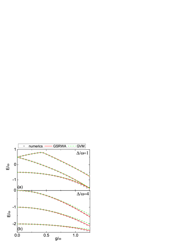
Figure 1: (Color online) Energy levels $E_{n}/\omega$ in the isotropic case as a function of $g/\omega$ for $\Delta/\omega=1$(a) and $\Delta/\omega=4$ (b) by means of the GSRWA (solid lines), numerical simulation (circles), GVM (dash-dotted lines) and GRWA (dashed lines)for the isotropic case $\tau=1$.

The energy levels from the numerical solution of the full Hamiltonian ( 2), the GVM, and the GSRWA are plotted for the isotropic case $\tau=1$ in Fig. 1. The GSRWA with optimal displacement $\beta$ in Eq.( 18)and squeezing $\lambda$ in Eq.( 17) captures the behavior of energy levels, and provides an agreement with the numerical ones ranging from the ultra-strong to npDSC regimes. The GVM with only the displacement transformation produces the correct behavior in the ultra-strong coupling regime, but breaks down in the npDSC regime $g/\omega>0.7$. The failure becomes more pronounced as the atom frequency $\Delta/\omega$ increases up to $4$ in Fig. 1(b), displaying a noticeable divergence of the GVM. It reveals that the displaced state is not a reasonable treatment in the npDSC regime, where the displaced-squeezed state is preferable and the deformation effects is appreciable.

Fig. 2 shows energy levels for the anisotropic Rabi case with relative weight $\tau=1.5$ and $0.5$ for the high-frequency atom $\Delta/\omega=4$. For small weight of the CRW interactions with $\tau=0.5$ in Fig. 2(a), the GSRWA is surprising robust as the coupling strength increases up to $g/\omega\sim 1.5$, where the energies in the GVM show dramatic deviation. Moreover, the GVM gets worse as the relative weight of the CRW terms increases to $\tau=1.5$ in Fig. 2(b). It exhibits an overall improvement of the GSRWA with the displaced-squeezed state to the GVM with the displaced state as the relative weight between the rotating-wave and CRW interactions increases . The advantage of our GSRWA lies in the contribution from the squeezing and displacement of the oscillator state. The GVM fails in particular to describe the eigenstates with the displaced state, which should be more sensitive in characterize the squeezing effects and the quantum dynamics presented in the following.

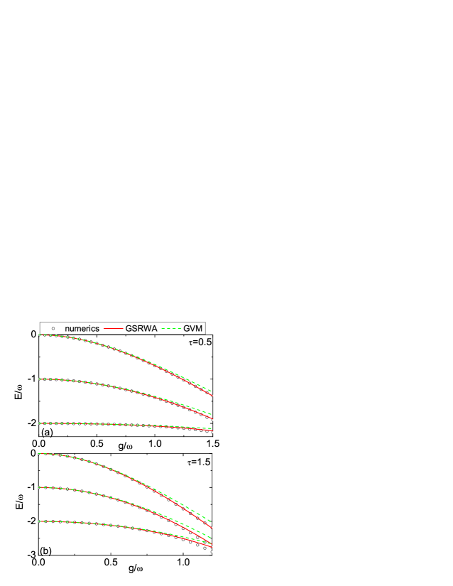
Figure 2: (Color online) Energy-level crossing as a function of $g/\omega$ in the anisotropic Rabi case (a) $\tau=0.5$ (b) $\tau=1.5$ for the detuning parameter $\Delta/\omega=4$ by means of the GSRWA (solid lines), numerical simulation (circles), GVM (dash-dotted lines) for the anisotropic case $\tau=0.5$.

IV Squeezing effects

We analyze the displaced-squeezed state in the GSRWA to explore the deformation or squeezing effects, which are described by the quadrature variance for momentum operator in the ground state. The ground state for the GSRWA is just as in the RWA giving by $|0\rangle|-z\rangle$. The operators expectation values of the ground state follows that

$$\langle a\rangle = \langle-z|\langle 0|SUaU^{\dagger}S^{\dagger}|0\rangle|-z\rangle$$ (27)

$$= \langle 0|a^{\dagger}\sinh 2\lambda+a\cosh 2\lambda|0\rangle-\beta$$

$$= -\beta,$$

and

$$\langle a^{\dagger}a\rangle = \langle-z|\langle 0|SUa^{\dagger}U^{\dagger}S^{\dagger}SUaU^{\dagger}S^{\dagger}|0\rangle|-z\rangle$$ (28)

$$= \sinh^{2}2\lambda+\beta^{2}.$$

The variance $\Delta p$ of the momentum $p=i\sqrt{\frac{\omega}{2}}(a^{\dagger}-a)$ can be determined from these expectation values, so that

$$\Delta p = \langle p^{2}\rangle-\langle p\rangle^{2}$$ (29)

$$= -\frac{\omega}{2}\langle a^{\dagger 2}+a^{2}-2a^{\dagger}a-1\rangle$$

$$= \frac{\omega}{2}e^{-4\lambda}.$$

Similarly, the variance $\Delta x$ of the position $x=(a^{\dagger}+a)/\sqrt{2\omega}$ is given by $\Delta x=e^{4\lambda}/(2\omega)$. The uncertainty in the momentum and position variables are therefore easily obtained as $\Delta p\Delta x=1/2$, which satisfy the minimum-uncertainty relation for the displaced-squeezed state.

Meanwhile, the variance of momentum $\Delta p$ in the GVM equals to $0.5$, which can be obtained easily from Eq.( 29) with the displaced state. Fig. 3 displays that the momentum variance by the GSRWA is smaller than $0.5$, indicating that the momentum quadrature is squeezed with the displaced-squeezed state. The quantum fluctuations in momentum variable are reduced at the expense of the corresponding increased fluctuations in the position variable such that the uncertainty relation is not violate. The squeezing effect is accurately captured by the displaced-squeezed state.

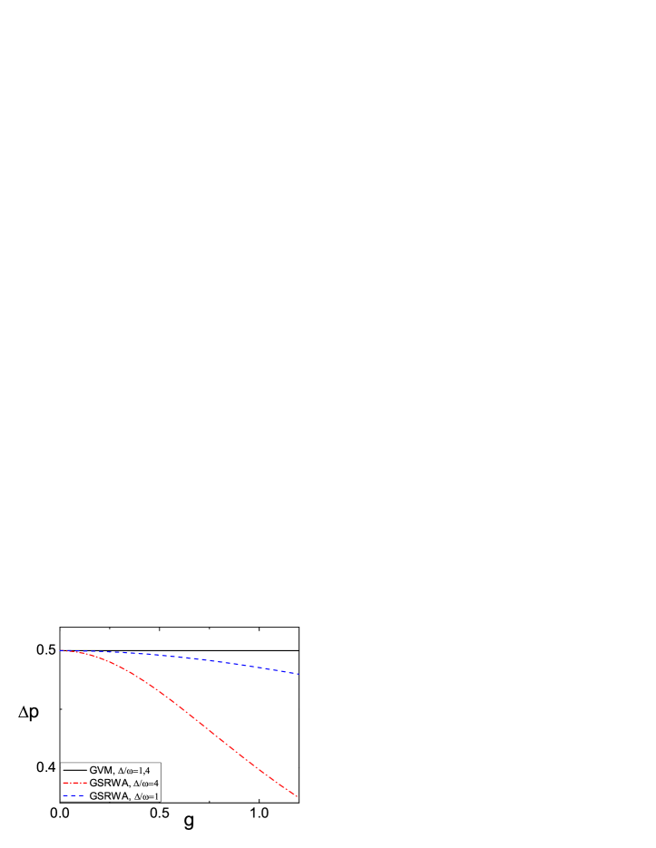
Figure 3: (Color online) Squeezing effect with the momentum variance $\Delta p$ as a function of $g$ for different atom frequency $\Delta/\omega=1$ (green dashed line) and $\Delta/\omega=4$ (red dashed-dotted line) obtained by the GSRWA and the GVM (black solid line) in the isotropic case.

V Population dynamics

The dynamical behavior of the two-level atom is of particular interest. In this section we explore the atomic population dynamics in the anisotropic Rabi model to test the accuracy of the energies and eigenstates in the npDSC regimes.

The initial state is taken to be $|\varphi(0)\rangle=|-x\rangle|\alpha_{-1}\rangle$ with the coherent state for the oscillator $|\alpha_{-1}\rangle=e^{\beta(a^{\dagger}-a)}|\alpha\rangle$. The wave function evolutes as $|\varphi(t)\rangle=e^{-iHt}|\varphi(0)\rangle$, which can be expanded by the eigenvalues $\{E_{n}\}$ ( 20) and eigenstates $\{|\Psi_{\pm,n}\rangle\}$ in Eqs.( III) and ( III) in the GSRWA.

The population for the atom remaining in the initial state $|-x\rangle$ is given by $P_{-1}(t)=|\langle-x|\mathtt{Tr}_{\mathtt{ph}}|\varphi(t)\rangle\langle\varphi(t)|-x\rangle|$, which is derived explicitly in the Appendix C. From the population formula in Eq.( 42), function $S_{n}$ displays the frequency of the Rabi’s oscillation depending on the transition frequencies $\Delta E_{m,n}^{j,j^{\prime}}=E_{j,m}-E_{j^{\prime},n}$ with $m=n,n-1$ ($j,j^{\prime}=\pm$).

Figure  4 shows the population $P_{-1}(t)$ as a function of the scaled time $\Delta t/2\pi$ at npDSC strength $g/\omega=0.5$ for high-frequency atom $\Delta/\omega=4$. We compare exact numerical results to the GSRWA and the GVM. Obviously, qualitative agreement between the GSRWA and the numerical ones of the dynamics oscillation is quite good even for long time scale for the isotropic and anisotropic Rabi model. However, the results in the GVM are quite different from the numerical ones. Apart from the energy levels, also the eigenstates become now of importance. The failure of population dynamics by the GVM is due to the breaks down of the displaced state in the npDSC regime, where the displaced-squeezed state is more stable to capture dynamics.

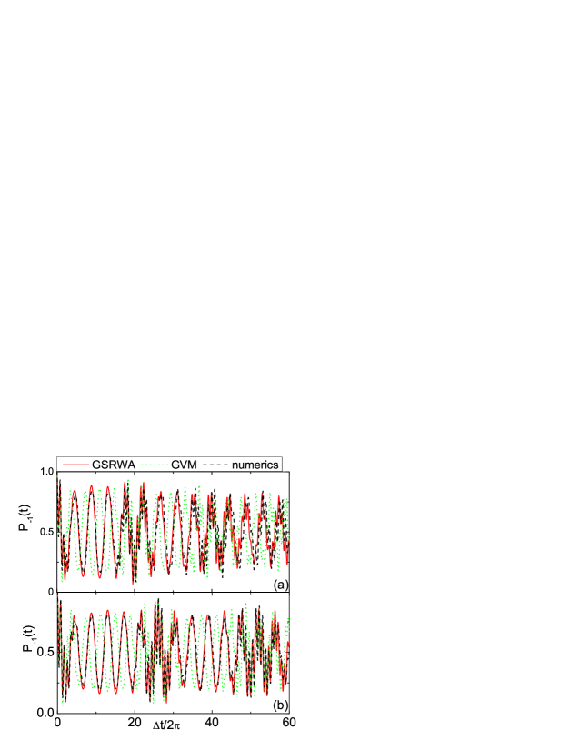
Figure 4: (Color online) Population $P_{-1}(t)$ for the coupling strength $g/\omega=0.5$ for the isotropic case $\tau=1$(a) and anisotropic case $\tau=0.5$ (b) by means of the GSRWA (solid lines), numerical simulation (circles), GVM (dash-dotted lines) and GRWA (dashed lines).

VI conclusion

We study the anisotropic Rabi model analytically in the nonperturbative DSC regime, belonging to the region between the ultra-strong and perturbative DSC coupling regimes. The GSRWA is performed by adding a squeezing transformation to the existing solutions with only the displacement transformation, giving an solvable Hamiltonian in the same form of the standard RWA. Energy levels obtained by the GSRWA agree well with numerical ones in a wide range of coupling strength, whereas the previous results show distinguished deviation in the nonperturbative DSC. Due to the displaced-squeezed state, the squeezed momentum variance displays the deformation effects induced by the atom-cavity coupling, which is omitted in the previous methods with the displaced state. And the population dynamics by the GSRWA is robust in the nonperturbative DSC regime even for high-frequency atom. The advantage of our GSRWA is not only substantial improvement of energy levels but also the stability of the displaced-squeezed oscillator state. Our approach provides an easy-to-implement analytical solutions to qubit-oscillator coupling systems currently for ultra-strong and perturbative DSC strengths, and also motivates further studies of multi-modes spin-boson model.

Appendix A Expanding of even and odd function

Since $\cosh\left[2\beta\eta\left(a^{\dagger}-a\right)\right]$ is expanded as $G^{0}\left(a^{\dagger}a\right)+G^{2}\left(a^{\dagger}a\right)a^{\dagger 2}+a^{2}G^{2}\left(a^{\dagger}a\right)+O(\beta^{4}\eta^{4})$, coefficient $G_{2}\left(a^{\dagger}a\right)$ of the two-excitation terms can be derived in the oscillator basis $|n\rangle$ as

$$G_{n+2,n}^{2} = \frac{1}{\sqrt{(n+2)(n+1)}}\langle n+2|\cosh[2\beta\eta\left(a^{\dagger}-a\right)]|n\rangle$$ (30)

$$= \frac{4\beta^{2}\eta^{2}}{(n+2)(n+1)}e^{-2\beta^{2}\eta^{2}}L_{n}^{2}(4\beta^{2}\eta^{2}).$$

Similarily, coefficients $T(a^{\dagger}a)$, $D_{0}\left(a^{\dagger}a\right)$ and $D_{2}\left(a^{\dagger}a\right)$ in the odd function $\left(a^{\dagger}-a\right)\cosh[2\beta\eta\left(a^{\dagger}-a\right)]$ and even function $\left(a^{\dagger}-a\right)\sinh[2\beta\eta\left(a^{\dagger}-a\right)]$ are given as $T_{n+1,n}$, $D_{n,n}^{0}$ and $D_{n+2,n}^{2}$ respectively

$$T_{n+1,n} = \frac{1}{\sqrt{n+1}}\left\langle n+1\right|\left(a^{\dagger}-a\right)\cosh[2\beta\eta\left(a^{\dagger}-a\right)]|n\rangle$$ (31)

$$= G_{n,n}^{0}-(n+2)G_{n+2,n}^{2},$$

$$D_{n,n}^{0} = \langle n|\left(a^{\dagger}-a\right)\sinh[2\beta\eta\left(a^{\dagger}-a\right)]|n\rangle$$ (32)

$$= -\sqrt{n}F_{n-1,n}(n)-\sqrt{n+1}F_{n+1,n}(n),$$

and

$$D_{n+2,n}^{2} = \frac{\langle n+2|\left(a^{\dagger}-a\right)\sinh[2\beta\eta\left(a^{\dagger}-a\right)]|n\rangle}{\sqrt{(n+1)(n+2)}}$$

$$= F_{n+1,n}(n)-\frac{\sqrt{n+3}}{\sqrt{(n+1)(n+2)}}F_{n+3,n}(n),$$

with $F_{n+3,n}(n)=\langle n+3|\sinh[2\beta\eta\left(a^{\dagger}-a\right)]|n\rangle=(2\beta\eta)^{3}e^{-2\beta^{2}\eta^{2}}L_{n}^{3}(4\beta^{2}\eta^{2})/\sqrt{(n+1)(n+2)(n+3)}$.

Appendix B Solution equations of $\lambda$ and displacement $\beta$

To obtain the optimal squeezing parameter $\lambda$ and displacement $\beta$ from Eqs.( 15) and ( 16), it is equivalent to solve the equations in detail

$$0 = (\alpha-\omega\beta)\eta_{3}-\frac{\Delta\beta\eta}{n+1}e^{-2\beta^{2}\eta^{2}}L_{n}^{1}(4\beta^{2}\eta^{2})$$ (34)

$$+\gamma\eta e^{-2\beta^{2}\eta^{2}}[L_{n}(4\beta^{2}\eta^{2})-\frac{4\beta^{2}\eta^{2}}{n+1}L_{n}^{2}(4\beta^{2}\eta^{2})],$$

$$0 = \eta_{2}-\frac{2\Delta\beta^{2}\eta^{2}}{(n+2)(n+1)}e^{-2\beta^{2}\eta^{2}}L_{n}^{2}(4\beta^{2}\eta^{2})$$ (35)

$$+\gamma\eta e^{-2\beta^{2}\eta^{2}}[\frac{2\beta\eta}{n+1}L_{n}^{1}(4\beta^{2}\eta^{2})$$

$$-\frac{(2\beta\eta)^{3}}{(n+1)(n+2)}e^{-2\beta^{2}\eta^{2}}L_{n}^{3}(4\beta^{2}\eta^{2})].$$

When the parameters $\lambda$ and $\beta$ are small compared with the unit, the associated Lagurre polynomial is given approximately by $L_{n}^{1}(4\beta^{2}\eta^{2})\simeq n+1,$ $L_{n}^{2}(4\beta^{2}\eta^{2})\simeq(n+1)(n+2)/2$ and $L_{n}^{3}(4\beta^{2}\eta^{2})\simeq(n+1)(n+2)(n+3)/3!$. Thus the above nolinear equations are simplified as

$$0 = (\alpha-\omega\beta)-\Delta\beta e^{-4\lambda}e^{-2\beta^{2}\eta^{2}}$$ (36)

$$+\gamma e^{-4\lambda}[1-2(n+2)\beta^{2}\eta^{2}]e^{-2\beta^{2}\eta^{2}},$$

and

$$0 = (e^{4\lambda}-e^{-4\lambda})-4\Delta\beta^{2}e^{-4\lambda}e^{-2\beta^{2}\eta^{2}}$$ (37)

$$+4\gamma e^{-4\lambda}[2\beta-\frac{4}{3}(n+4)\beta^{3}e^{-4\lambda}]e^{-2\beta^{2}\eta^{2}}.$$

Appendix C Analytical expression of population

The wave function $|\varphi(t)\rangle$ can be expanded by the eigenvalues $\{E_{n}\}$ and eigenstates $\{|\Psi_{\pm,n}\rangle\}$ as

$$|\varphi(t)\rangle=f_{0}e^{-iE_{0}t}|\Psi_{0}\rangle+\sum_{n=0}f_{\pm,n}e^{-iE_{\pm,n}t}|\Psi_{\pm,n}\rangle,$$ (38)

where the coefficients $f_{0}=\langle\Psi_{0}|\varphi(0)\rangle$ and $f_{\pm,n}=\langle\Psi_{\pm,n}|\varphi(0)\rangle$. And the overlap between the displaced-squeezed state and the initial coherent state is expressed by the polynomials

$${}_{-,ds}\langle n|\alpha_{-1}\rangle$$

$$= \chi\sum_{i=0}^{n/2}\frac{(-0.5\tanh 2\lambda)^{i}}{i!(n-2i)!}e^{(n-2i+1/2)In\sec h2\lambda}(-\alpha)^{n-2i}$$

with $\mu=e^{2\lambda}$, $\sec h(2\lambda)=\frac{2\mu}{1+\mu^{2}}$and $\tanh(2\lambda)=\frac{\mu^{2}-1}{1+\mu^{2}}$, and $\chi=\sqrt{n!}e^{-\alpha^{2}/2}e^{\frac{\alpha^{2}}{2}\tanh 2\lambda}$. Thus, the coefficient $C_{-x}$ of the atom state $|-x\rangle$ is

$$C_{-x} = (\kappa_{0}e^{-iE_{0}t}+\kappa_{+,0}e^{-iE_{+,0}t}+\kappa_{-,0}e^{-iE_{-,0}t})|0\rangle_{-,ds}$$

$$+\sum_{n>0,j=\pm}(\kappa_{j,n-1}e^{-iE_{j,n-1}t}+\kappa_{j,n}e^{-iE_{j,n}t})|n\rangle_{-,ds},$$

where coefficients are given as $\kappa_{0}=f_{0}/\sqrt{2}$, $\kappa_{+,n}=\cos\frac{\theta_{n}}{2}f_{+,n}/\sqrt{2}$ , $\kappa_{-,n-1}=-\cos\frac{\theta_{n-1}}{2}f_{-,n}/\sqrt{2}$, $\kappa_{+,n-1}=\sin\frac{\theta_{n-1}}{2}f_{+,n}/\sqrt{2}$ and $\kappa_{-,n}=\sin\frac{\theta_{n}}{2}f_{-,n}/\sqrt{2}$. The population $P_{-1}(t)=|C_{-x}^{\ast}C_{-x}|$ for the atom remaining in the initial state $|-x\rangle$ is expressed as

$$P_{-1}(t) = \kappa_{0}\kappa_{+,0}\cos[(E_{0}-E_{+,0})t]$$ (42)

$$+\kappa_{0}\kappa_{-,0}\cos[(E_{0}-E_{-,0})t]$$

$$+\kappa_{+,0}\kappa_{-,0}\cos[(E_{-,0}-E_{+,0})t]$$

$$+\sum_{n>0}S_{n}(t)+k,$$

where

$$S_{n}(t) = \sum_{j,j^{\prime}=\pm}\kappa_{j,n}\kappa_{j^{\prime},n}\cos\Delta E_{n,n}^{j,j^{\prime}}+\kappa_{j,n-1}\kappa_{j^{\prime},n}\cos\Delta E_{n-1,n}^{j,j^{\prime}}$$ (43)

$$+\kappa_{j,n-1}\kappa_{j^{\prime},n-1}\cos\Delta E_{n-1,n-1}^{j,j^{\prime}}$$

with $\Delta E_{m,n}^{j,j^{\prime}}=E_{j,m}-E_{j^{\prime},n}$, ($m=n,n-1$) and the constant $k=\kappa_{0}^{2}+\kappa_{+,0}^{2}+\kappa_{-,0}^{2}$

References

- (1) I. I. Rabi, Phys. Rev. 51,652 (1937).
- (2) E.T. Jaynes, and F.W. Cummings, Proc. IEEE. 51, 89(1963).
- (3) P. Forn-Díaz, et al., Nature Physics 39, 13 (2016).
- (4) F. Yoshihara, et al., Nature Physics 44, 13 (2016).
- (5) A. Wallraff et al., Nature (London)431, 162(2004).
- (6) T. Niemczyk et al., Nature Physics 6, 772(2010).
- (7) P. Forn-Díaz et al., Phys. Rev. Lett. 105, 237001 (2010).
- (8) A. Fedorov et al., Phys. Rev. Lett. 105, 060503 (2010).
- (9) J. Casanova, G. Romero, I. Lizuain, J. J. Garcia-Ripoll, and E. Solano, Phys. Rev. Lett. 105, 263603(2010).
- (10) S. De Liberato, Phys. Rev. Letter 112, 016401 (2014).
- (11) S. I. Erlingsson, J. C. Egues, and D. Loss, Phys. Rev. B 82, 155456(2010).
- (12) Y. Yi-Xiang, J. W. Ye, and W. M. Liu, Sci. Rep. 3, 3476(2013).
- (13) Q. T. Xie, S. Cui, J. P. Cao, L. Amico, and H. Fan, Phys. Rev. X 4, 021046(2014).
- (14) L. T. Shen, et al., Phys. Rev. A. 95, 013819(2017).
- (15) Y. Zhang, G. Chen, L. Yu, Q. Liang, J. Q. Lang, and S. T. Jia, Phys. Rev. A 83, 065802 (2011).
- (16) C. J. Gan, and H. Zheng, Eur. Phys. J. D 59,473 (2010).
- (17) E.K. Irish, Phys. Rev. Lett. 99, 173601(2007).
- (18) Y. Y. Zhang, Q. H. Chen, and Y. Zhao, Phys. Rev. A 87, 033827(2013); Y. Y. Zhang, Q. H. Chen, ibid 91, 013814(2015).
- (19) S. Agarwal, S. M. Hashemi Rafsanjani, and J. H. Eberly, Phys. Rev. A 85, 043815 (2012).
- (20) S. Ashhab, Phys. Rev. A 87, 013826 (2013).
- (21) Z. J. Ying, M. X. Liu, H. G. Luo, H. Q. Lin, and J. Q. You,Phys. Rev. A 92, 053823 (2015).
- (22) M. J. Hwang, R. Puebla, and M. B. Plenio, Phys. Rev. Lett. 115, 180404 (2015).
- (23) D. Z. Rossatto, et al., Phys. Rev. A 96, 013849 (2017).
- (24) A. L. Boité, Phys. Rev. A 94, 033827 (2016).
- (25) Y. Y. Zhang, Phys. Rev. A. 94, 063824(2016).
- (26) L. Cong, et al., Phys. Rev. A. 95, 063803(2017).